the Creative Commons Attribution 4.0 License.
the Creative Commons Attribution 4.0 License.
 | 17 Feb 2023
Monitoring Arctic thin ice: a comparison between CryoSat-2 SAR altimetry data and MODIS thermal-infrared imagery
Felix L. Müller
Stephan Paul
Stefan Hendricks
Denise Dettmering
Areas of thin sea ice in the polar regions not only are experiencing the highest rate of sea-ice production but also are, therefore, important hot spots for ocean ventilation as well as heat and moisture exchange between the ocean and the atmosphere. Through co-location of (1) an unsupervised waveform classification (UWC) approach applied to CryoSat-2 radar waveforms with (2) Moderate Resolution Imaging Spectroradiometer-derived (MODIS) thin-ice-thickness estimates and (3) Sentinel-1A/B synthetic-aperture radar (SAR) reference data, thin-ice-based waveform shapes are identified, referenced, and discussed with regard to a manifold of waveform shape parameters. Here, strong linear dependencies are found between binned thin-ice thickness up to 25 cm from MODIS and the CryoSat-2 waveform shape parameters that show the possibility of either developing simple correction terms for altimeter ranges over thin ice or directing adjustments to current retracker algorithms specifically for very thin sea ice. This highlights the potential of CryoSat-2-based SAR altimetry to reliably discriminate between occurrences of thick sea ice, open-water leads, and thin ice within recently refrozen leads or areas of thin sea ice. Furthermore, a comparison to the ESA Climate Change Initiative's (CCI) CryoSat-2 surface type classification with classes sea ice, lead, and unknown reveals that the newly found thin-ice-related waveforms are divided up almost equally between unknown (46.3 %) and lead type (53.4 %) classifications. Overall, the UWC results in far fewer unknown classifications (1.4 % to 38.7 %). Thus, UWC provides more usable information for sea-ice freeboard and thickness retrieval and at the same time reduces range biases from thin-ice waveforms processed as regular sea ice in the CCI classification.
- Article
(7614 KB) - Full-text XML
- BibTeX
- EndNote


Areas of thin-sea-ice cover in the polar regions play an important role for sea-ice production and heat exchange of the ocean with the atmosphere – especially during polar night (e.g. Meier et al., 2014; Morales Maqueda et al., 2004; Maykut, 1978; Thorndike et al., 1975). Several studies investigated the presence of thin sea ice in leads and polynyas within the Arctic (e.g. Rothrock et al., 1999; Preußer et al., 2016, 2019; Tian-Kunze et al., 2014; Huntemann et al., 2014; Willmes et al., 2010; Willmes and Heinemann, 2015, 2016; Reiser et al., 2020). Leads and polynyas are openings of varying size and shape within the sea-ice scape and per definition of the World Meteorological Organization (WMO) may consist of not only open-water areas but also thin ice with a thickness of up to 30 cm (WMO, 2014). The studies investigating thin ice use different sensors and retrieval methodologies that are generally bound to an upper sea-ice-thickness limit and methodological limitations (e.g. snow cover and/or cloud-cover presence when using thermal-infrared data (e.g. Yu and Rothrock, 1996; Frey et al., 2008) or spatial resolution using passive-microwave data (e.g. Tamura et al., 2008)).
In contrast, satellite altimetry is capable of retrieving sea-ice freeboard and sea-ice thickness for the Arctic on a basin scale using CryoSat-2 and its predecessor sensors, with several data products already available (e.g. Landy et al., 2019; Paul et al., 2018; Guerreiro et al., 2017; Kurtz et al., 2014). However, studies suggest a higher uncertainty towards thinner sea ice (Ricker et al., 2017). This is the result of several factors. The radar backscatter characteristics between young and thin sea ice is ambiguous with open-water area, since both surfaces have specular reflection properties that lead to off-nadir reflection biasing the radar range (e.g. Aldenhoff et al., 2019; Passaro et al., 2018; Rinne and Similä, 2016). However, classifying radar waveform echoes by their respective backscattering surface type (i.e. sea ice, open ocean, or leads) is essential for the upstream process of retrieving sea-ice freeboard and sea-ice thickness using satellite radar altimetry (e.g. Laxon, 1994; Laxon et al., 2003; Peacock and Laxon, 2004). Numerous studies exist on the automatic detection of leads. These use altimeter data (e.g. Lee et al., 2018; Dettmering et al., 2018; Wernecke and Kaleschke, 2015) or synthetic-aperture radar (SAR) images (e.g. Park et al., 2020; Murashkin et al., 2018). A lead in the context of radar altimetry is an ice-free opening surrounded by sea ice that enables direct measurements of sea-surface height within the ice cover. However, none of the existing studies have yet attempted to detect thin ice using satellite altimetry data. Continuous sea-surface height observations over open ocean and at discrete lead locations are then interpolated along the track, and one can subsequently calculate the sea-ice freeboard (i.e. the instantaneous height differences between the sea-ice surface and the ocean surface). Assuming hydro-static equilibrium and utilizing additional auxiliary information on sea-ice type and respective sea-ice density, as well as information on the sea-ice snow cover, one can calculate the sea-ice thickness (e.g. Paul et al., 2018; Alexandrov et al., 2010).
For correct sea-ice classifications, the small freeboard values of thin ice (here defined as sea ice with a thickness up to 25 cm) are often lower than the precision of even the recent synthetic-aperture radar (SAR) altimeter sensors. In addition, freeboard estimates of sea ice from Ku-band radar altimeters must be adjusted for a lower wave propagation speed in the snow layer (Mallett et al., 2020). In the absence of a direct observation for each radar altimeter waveform, snow depth and density information may originate from a climatology, modelled snow depth with reanalysis as input, or data fusion of different satellite sensors. However, all approaches provide an average snow depth for a certain period and region, which will overestimate the snow layer on young sea ice in most cases and create a freeboard bias. Hence, there is currently a need for additional satellite products or physical waveform models to better understand retrievals based on radar altimeter waveforms over thin-ice areas to complement improvements for thicker and rougher sea-ice surfaces (e.g. Landy et al., 2019).
While information on the presence of thin-ice areas is important for our understanding of sea-ice mass balance changes, there are currently only two operational Arctic-wide thin-ice data products available due to the above-mentioned limitations. These products are both produced from ESA's Soil Moisture and Ocean Salinity (SMOS) mission (Huntemann et al., 2014; Tian-Kunze et al., 2014) based on the ice-thickness dependency of surface emissivity at the L band. However, this is at a lower spatial resolution of 12.5 km×12.5 km at best (Tian-Kunze et al., 2014). Both methods are limited for thicker sea ice above 0.5 m (Huntemann et al., 2014) or 1 m (Tian-Kunze et al., 2014), respectively. Thus, the latter product, as an official ESA product, is routinely used to improve sea-ice-thickness retrieval over the full range of the sea-ice-thickness distribution utilizing a data fusion approach between SMOS and CryoSat-2 using optimal interpolation (Ricker et al., 2017). Data products utilizing thermal-infrared data to estimate thin-ice thickness and corresponding areas are also available but not in a similar operational fashion (e.g. Preußer et al., 2016, 2019).
In this study, the authors utilize delay-Doppler radar altimeter echoes from ESA's Earth Explorer mission CryoSat-2 in combination with the capabilities of NASA's Moderate Resolution Imaging Spectroradiometer (MODIS) to allow for a better understanding of the received CryoSat-2 waveform returns over thin-sea-ice areas and, subsequently, an improved surface type classification. For this task, the authors intercompare CryoSat-2 waveforms labelled as thin ice through an unsupervised classification approach (extended from Müller et al., 2017) with thin-ice-thickness estimates from MODIS (Paul et al., 2015) within a maximum of 30 min between both acquisitions. Additionally, in Sect. 4.3 (“Classification comparison”), the authors show a statistical analysis of the results obtained by the unsupervised classification approach (Müller et al., 2017) and the classification used in the ESA Climate Change Initiative (CCI) described in Paul et al. (2018).
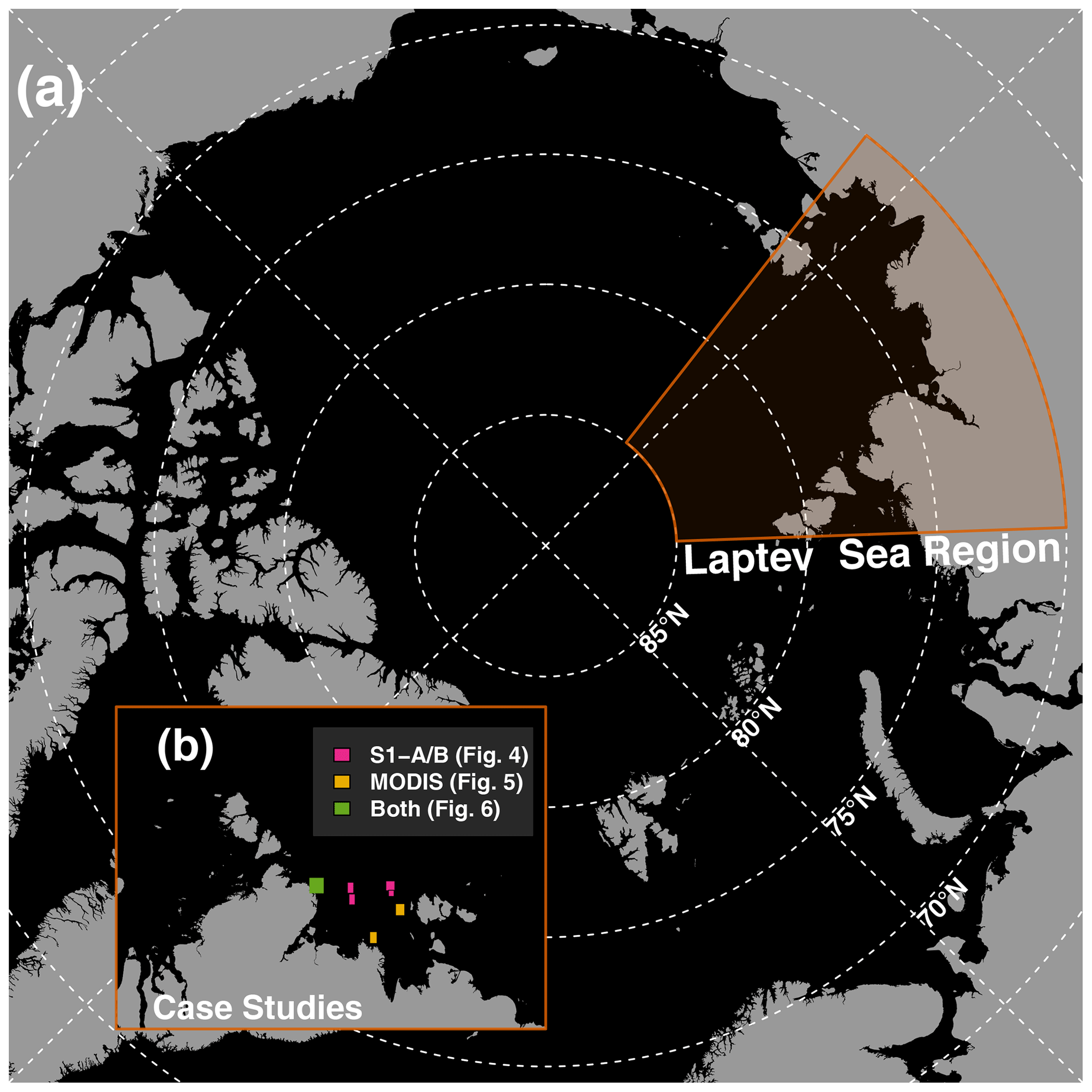
All investigations are performed for the Arctic Laptev Sea region featuring frequent occurrences of flaw and coastal polynyas, i.e. polynyas bound to fast ice or the coast, respectively (Fig. 1; e.g. Preußer et al., 2019; Willmes et al., 2010), and cover the winter months January through March between 2011 and 2020.
This study is structured into the following sections. Section 2 describes the data sets; Sect. 3 provides details on the unsupervised clustering for CryoSat-2 and the MODIS thin-ice-thickness retrieval. Section 4 summarizes and discusses the results and implications on CryoSat-2 surface type classification, and Sect. 5 concludes with an outlook.
The following subsection highlights the main data sets used for this study. All analyses are carried out for the Arctic Laptev Sea region between 70–85∘ N, 92–142∘ E (Fig. 1) for the winter months January through March between 2011 and 2020.
2.1 CryoSat-2 Level-1B Baseline-D data
CryoSat-2 was launched in April 2010 aiming to monitor Earth's cryosphere and, in particular, to measure the decline in land and sea ice in the polar regions in order to understand the role of climate in the retreat of polar ice. CryoSat-2 was placed on a non-Sun-synchronous orbit with a long repeat orbit of about 369 d. CryoSat-2 is carrying a Ku-band radar altimeter and is observing in three different acquisition modes up to a latitude of 88∘ N/S (Scagliola, 2013). The acquisition modes vary with application area and surface type with respect to a geographical mode mask (for more information, see https://earth.esa.int/eogateway/instruments/siral/description, last access: 14 February 2023).
The polar seas are predominantly sampled by the synthetic-aperture radar (SAR) mode with an along-track footprint size of about 300 m (Wingham et al., 2006). Briefly summarized, the SAR mode combines frequency-shifted radar returns (i.e. Doppler effect) in the direction of flight from different look angles with respect to a predefined position on the surface. The result of combining different view angles is called a multi-look waveform and samples the surface with 20 Hz resolution.
The present investigation is based solely on SAR-mode-acquired multi-looked waveforms, covering major parts of the Arctic Ocean. In particular, CryoSat-2 Level-1B (L1B) Ice Baseline-D data are introduced to the processing chain. This data set comprises, in addition to the waveform data, information on waveform scaling as well as orbit positions. More information regarding Baseline-D can be found in the ESA CryoSat-2 Product Handbook (Bouzinac, 2019) and Meloni et al. (2020).
2.2 MODIS data
For the comparison of thin-ice thickness to CryoSat-2 waveforms, MODIS Level-1B-calibrated radiances are obtained from both NASA satellites, Terra and Aqua (MOD/MYD02; MCST, 2017a, b), retrieved from the Level-1 and Atmosphere Archive and Distribution System (LAADS) Distributed Active Archive Center (DAAC) with a spatial resolution of 1 km×1 km at nadir and swath dimensions of 1354 km (across track) × 2030 km (along track).
Brightness temperatures were calculated from the calibrated radiances comprising MODIS channels 31 and 32 at 10.78 to 11.28 µm and 11.77 to 12.27 µm, respectively, following Toller et al. (2017). Subsequently, the sea-ice surface temperature (IST) was computed following Riggs and Hall (2015). All MODIS processing is based on MODIS Collection 6.1 data for nighttime only.
In order to compute corresponding thin-ice-thickness data from the IST data, additional data on the prevailing atmospheric conditions are necessary. Here, all necessary atmospheric fields are provided from the European Centre for Medium-Range Weather Forecasts (ECMWF) fifth-generation reanalysis (ERA5) data acquired from the Copernicus Climate Data Store (CDS; Hersbach et al., 2020). These fields comprise the 2 m air temperature, the 10 m wind-speed components, the mean sea-level pressure, and the 2 m dew-point temperature in hourly resolution.
2.3 Sentinel-1A/B SAR images
The ESA Copernicus C-band SAR missions Sentinel-1A and Sentinel-1B (S1-A/B) were launched in 2014 and 2016, respectively. At the time of full functionality, both satellites orbited Earth 180∘ apart to provide SAR imagery, unaffected by cloud cover, on a 6 d repeating cycle. SAR images from both missions are used for visual comparisons. Automatic thin-ice detection from SAR images is not applied in this study because this falls outside the main focus of the work. S1-A/B features a higher spatial resolution with regard to MODIS and, therefore, provides further information about different sea-ice surface types by making use of the backscattering properties of different surfaces. For instance, leads and polynyas appear very dark due to a very flat and less rough surface. In this case the incoming radar signal is scattered away from the receiver. However, caution must be taken by the interpretation of the backscattering pixel values in the presence of small-scale features like frost flowers (i.e. small ice crystals with the size of a few centimetres in diameter) that develop under cold and calm conditions, e.g. on nilas ice, as they can significantly increase the scattering resulting in brighter pixel values (Hollands and Dierking, 2016). Furthermore, brighter pixel values can also result from a roughened water surface due to strong wind influence in polynyas. More information regarding sea-ice surface type interpretation can be found in Dierking (2013) and Murashkin et al. (2018).
In the present study, the Sentinel-1 comparison data set consists of Level-1 dual-polarized SAR extra-wide-swath mode data at medium resolution. The images are ground range detected and show a pixel resolution of 40 m×40 m and a swath width of 400 km. The spatial resolution is close to 100 m. The images are processed using SNAP (ESA Sentinel Application Platform) v8.0 (http://step.esa.int, last access: 14 February 2023) following the processing steps described in Müller et al. (2017) and Passaro et al. (2018) but with an additional speckle filtering. Briefly summarized, the main processing steps follow standard routines (e.g. radiometric calibration, speckle filtering, map projection). The Level-1 data are gathered from the Alaska Satellite Facility Data Active Archive Center (ASF DAAC). In terms of the study area and period, the Sentinel-1A/B image pool represents a potentially usable size of approximately 500 scenes. Unfortunately, Sentinel-1B was decommissioned after an instrument failure in December 2021.
The following section focuses on the key steps of data processing that enable a comparison of thin-ice observations from SAR altimetry and MODIS thermal-infrared imagery. In order to reduce the influence of rapidly changing environmental conditions such as sea-ice drift, rapid melt, and freezing periods, the maximum time gap between altimetry, thermal-infrared imagery, and SAR imaging is set to ±30 min around the overflight times of CryoSat-2. This is a compromise to minimize observation situation changes while at the same time enabling a sufficiently large MODIS as well as SAR image database. This is necessary due to the frequent presence of cloud cover in the MODIS data. After setting a maximum permissible acquisition time difference between CryoSat-2 and Sentinel-1A/B, the number of possible SAR images is reduced to 52. Other limiting factors concern the actual number of overlap points in the image area. The images shown in Sect. 4.1 correspond to examples with a very good overlap and different surface conditions.
From ERA5 2 m air temperature data, the average temperatures for the study period and region are always well below the freezing point (about 253 K on average; Fig. 1). However, there are rare occasions of temperatures above the freezing point (about 1.6 % of all days within the study period) especially over land but also near the coast over sea-ice/fast-ice areas. While certainly the surface conditions change under these conditions and potentially impact the received returns for CryoSat-2, the overall impact on the unsupervised waveform classification (UWC) is considered negligible.
The MODIS comparison database includes 161 scenes, which corresponds to an altimetry data set of about 21 300 CryoSat-2 altimeter waveforms (MODIS scene numbers and their time difference from the CryoSat-2 tracks are available upon request).
3.1 CryoSat-2 thin-ice classification
Müller et al. (2017) developed an unsupervised classification of altimeter waveforms that was primarily focused on the detection of open-water targets, such as leads and polynyas, without the use of training data or previously known information about the surface conditions. The classification can be applied to any kind of altimeter waveforms and missions. Müller et al. (2017) applied it to the non-SAR, conventional altimeter missions Envisat and SARAL (Satellite with ARgos and ALtiKa). Later, the classification approach was adopted to SAR altimeter waveforms (Dettmering et al., 2018) and applied to CryoSat-2 and Sentinel-3A/B in the framework of the European Space Agency's Baltic+ Sea Level (ESA Baltic SEAL) project (Passaro et al., 2021). However, none of these studies classified thin ice, since altimeter waveforms generated by this surface type are quite similar to open-water returns.
Briefly summarized, the unsupervised waveform classification (UWC) is based on an automatic clustering of a broad spectra of different waveforms by K-medoids classification (e.g. Celebi, 2014) defining a reference model with a certain number of clusters. After clustering, an assignment of the clustered waveforms as well as remaining waveforms to certain surface types (e.g. ocean, lead/polynya, or sea-ice conditions) is performed. The assignment of the waveform clusters to the different surface types is mainly based on the use of background knowledge about the physical backscattering properties of the individual surface types and statistical relationships (Fig. 2). More detailed explanations of the cluster assignment can be found in Müller et al. (2017). In the present investigation, the cluster number is set to 25. This number was found to produce optimal results in Dettmering et al. (2018) and led there to an overall agreement of about 97 %. Moreover, an internal misclassification rate of 1.13 % can be expected after performing a 10-fold cross validation (Passaro et al., 2020).
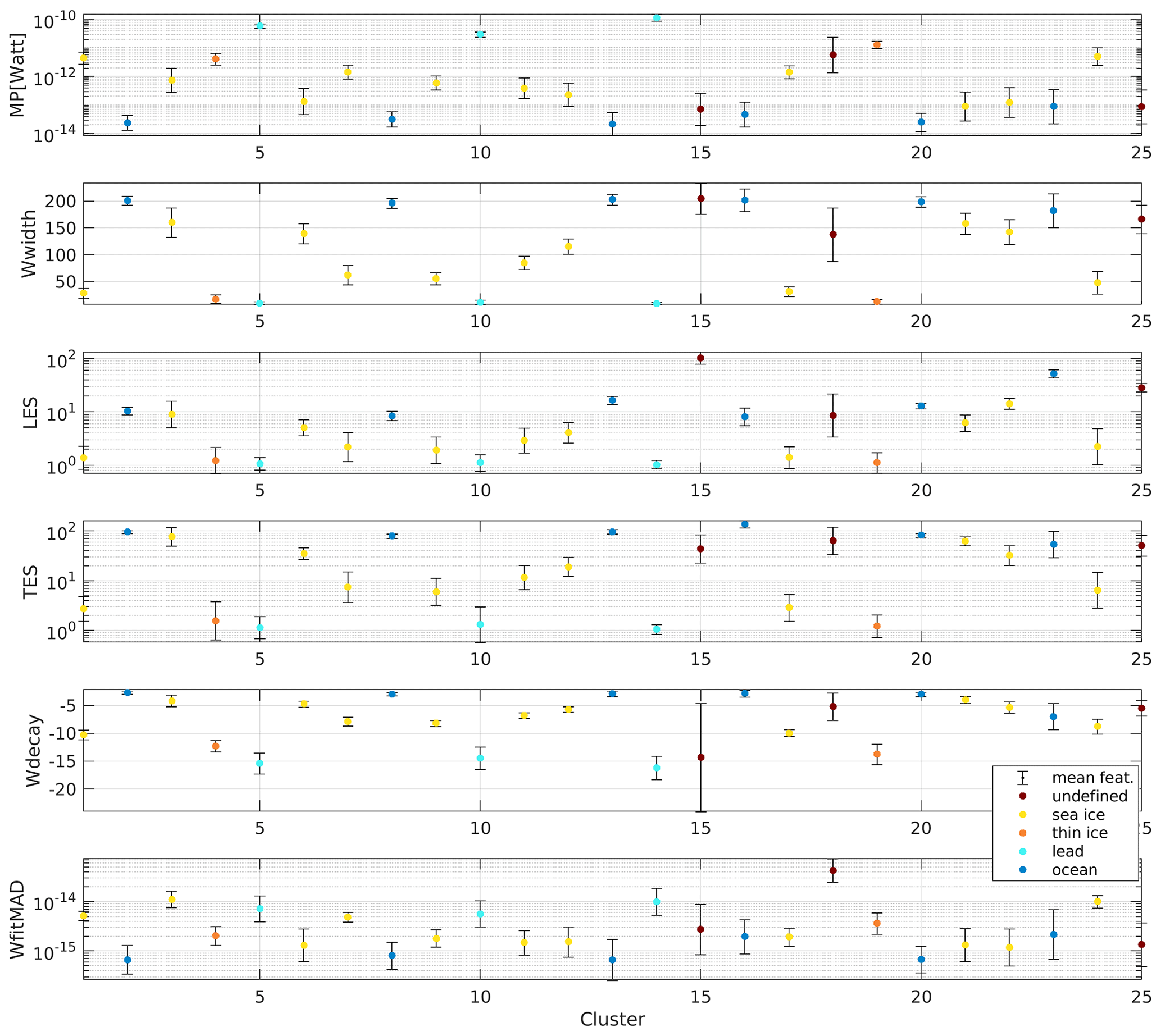
Figure 2Averages and standard error of six waveform features used per cluster: maximum power (MP), waveform width (Wwidth), leading-edge slope (LES), trailing-edge slope (TES), waveform decay (Wdecay), and median absolute deviation of fitted waveforms (WfitMAD). Colours indicate five different surface types: undefined (brown), sea ice (yellow), thin ice (orange), lead (cyan), and ocean (blue).
The main input to the classification approach is parameters derived from the waveform shapes and information on the backscatter power. Altogether, they span the feature space, which is defined as follows (see Dettmering et al., 2018):
-
Maximum power (MP) – physical backscatter coefficient σ0 at the waveform maximum
-
Waveform width (Wwidth) – number of waveform range bins with a power greater than 1 % of the waveform maximum
-
Leading-edge slope (LES) – number of waveform range bins between the position of the waveform maximum and the bin of the leading edge, which is the first exceeding 12.5 % of the maximum power
-
Trailing-edge slope (TES) – similar to LES but for the trailing edge of the waveform
-
Waveform decay (Wdecay) – estimation of the decay by fitting an exponential function to the trailing edge
-
Waveform fit median absolute deviation (WfitMAD) – derived MAD value of the residuals from the fit of the exponential function.
Moreover, in the quantitative comparison (Sect. 4.2) two additional features are included. The additional features are part of the CryoSat-2 waveform classification approach (Paul et al., 2018) applied in the framework of ESA CCI:
-
Leading-edge width (LEW) – width in range bins between 95 % and the first bin at the leading edge exceeding 5 % of the waveform maximum power using a 10-time oversampled and smoothed waveform (Hendricks et al., 2021)
-
Leading-edge peakiness (LEP) – computation of the pulse peakiness (Peacock and Laxon, 2004) but with three range bins left from the bin position of the waveform maximum (Ricker et al., 2014).
Figure 2 shows the assignment of 25 clusters to 5 different surface types (compared to 4 in the original UWC approach): undefined, sea ice, thin ice, lead, and ocean. Clusters characterized by a very strong MP, a small Wwidth, and strong decay obtained by the fitting of an exponential function to the trailing edge of the waveform are labelled as lead clusters (i.e. 5, 10, 14). Clusters that were formerly assigned to sea ice are now divided into two groups (sea ice and thin ice) based on their different reflective properties. Following Ulander et al. (1995) and Onstott and Shuchman (2004) thin ice covers nilas and young ice ranging from 0 to 0.30 m and is often covered by a flat layer of slush, which is ice crystals saturated with salt brine. Members of thin-ice clusters show characteristics in between lead clusters and clear sea-ice groups. They are characterized by a wider waveform shape, a weaker waveform decay, and a flatter trailing-edge slope than lead clusters. Moreover, they also have a slightly weaker MP than radar returns reflected from open, calm water (Zygmuntowska et al., 2013). These properties correspond to clusters 4 and 19.
Undefined waveform clusters represent waveforms which cannot assigned unambiguously to certain surface conditions, for example if they are acquired in the direct vicinity of the coast or islands. They also show a bigger standard deviation compared to other clusters.
3.2 MODIS thin-ice-thickness retrieval
In order to compute the thin-ice thickness (TIT) from MODIS IST a simple surface energy balance model is employed, which utilizes the inversely proportional relation between IST and the thickness of thin sea ice (Yu and Rothrock, 1996; Drucker et al., 2003). In the model, the net positive flux towards the atmosphere (i.e. positive corresponding to the direction from the warm ocean to the cold atmosphere) is equalized from the conductive heat flux through the ice. From this conductive heat flux, TIT is derived following Eq. (1), where TIT is the thin-ice thickness; κi is the thermal conductivity of sea ice (2.03 W (m K)−1); IST and Tfp are the IST and the ice–ocean interface temperature (assumed to be at the freezing point of the ocean), respectively; and Qatm is the total heat flux to the atmosphere.
A detailed description of the TIT retrieval procedure as well as all necessary equations and related assumptions are thoroughly described in Paul et al. (2015). These assumptions comprise the following: sea ice that is free of snow cover, a linear temperature gradient within the sea ice, a negligible ocean-heat flux, and cloud-free conditions assured by manual screening of all used MODIS swaths (Paul et al., 2015). While no state-of-the-art uncertainty analysis is available for our combination of MODIS thin-ice retrieval with ERA5 atmospheric reanalysis, Adams et al. (2012) state an average uncertainty of ±4.7 cm for ice thicknesses between 0.0 and 0.2 m using the NCEP2 reanalysis (National Centers for Environmental Prediction; Kalnay et al., 1996), substantially increasing for larger thickness ranges. Figure 3 exemplifies the underlying IST with its corresponding TIT. With regard to these uncertainty limitations in combination with the desire to maximize CryoSat-2/MODIS overlaps, all TIT analyses are limited to a maximum sea-ice thickness of 25 cm.
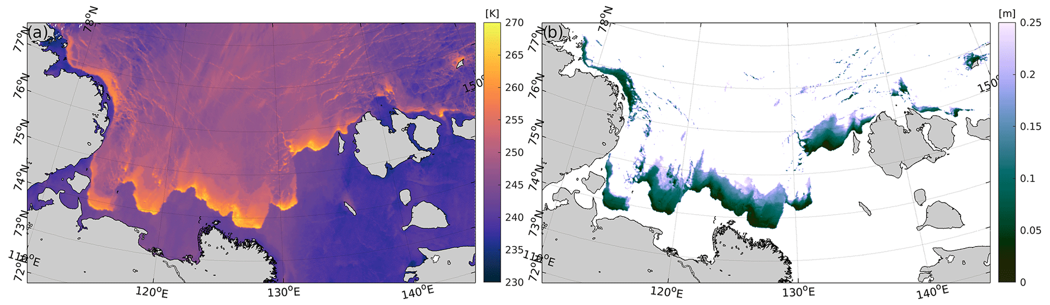
Figure 3Example of MODIS ice-surface temperature (IST in K; a) and its associated thin-ice thickness (TIT; b) between 0 and 0.25 m, as acquired on 5 March 2011 at 18:10 UTC.
In this study, a combination of 161 MODIS swaths covering the Laptev Sea area showing TIT up to 25 cm and about 21 300 classified CryoSat-2 observations are used for a quantitative analysis. The very high-spatiotemporal-resolution altimetry observations are related to the respective MODIS pixels using a nearest-neighbour approach. Moreover, Sentinel-1A/B SAR images serve as an additional source for visual comparisons. The first part of this section shows visual comparisons between CryoSat-2 and MODIS as well as Sentinel-1. The second part (Sect. 4.2) will then focus on a quantitative analysis of the results. In the last part, Sect. 4.3 briefly evaluates the representation of thin-ice class waveforms in other CryoSat-2-based products (Paul et al., 2018) compared to the unsupervised classification approach.
A direct comparison to SMOS-derived sea-ice thicknesses (Tian-Kunze et al., 2014) is of limited use due to (i) it being an average daily ice-thickness product on a spatial resolution of 12.5 km×12.5 km and (ii) the product's setup with its use of a statistical log-normal ice-thickness distribution (Tian-Kunze et al., 2014). The latter results in the real level-ice thickness being more likely about half of the shown numbers. However, this renders this data set unusable for the purpose of this study as the actual ice thickness of thin sheet ice is needed for the comparison to the high-resolution CryoSat-2 data (Fig. A1).
4.1 Visual comparison
This section provides an initial visual intercomparison between CryoSat-2 classified open-water lead, thin-ice, and sea-ice observations on the one hand and either MODIS (Table A1) or Sentinel-1A/B SAR imagery (Table A2) on the other hand.
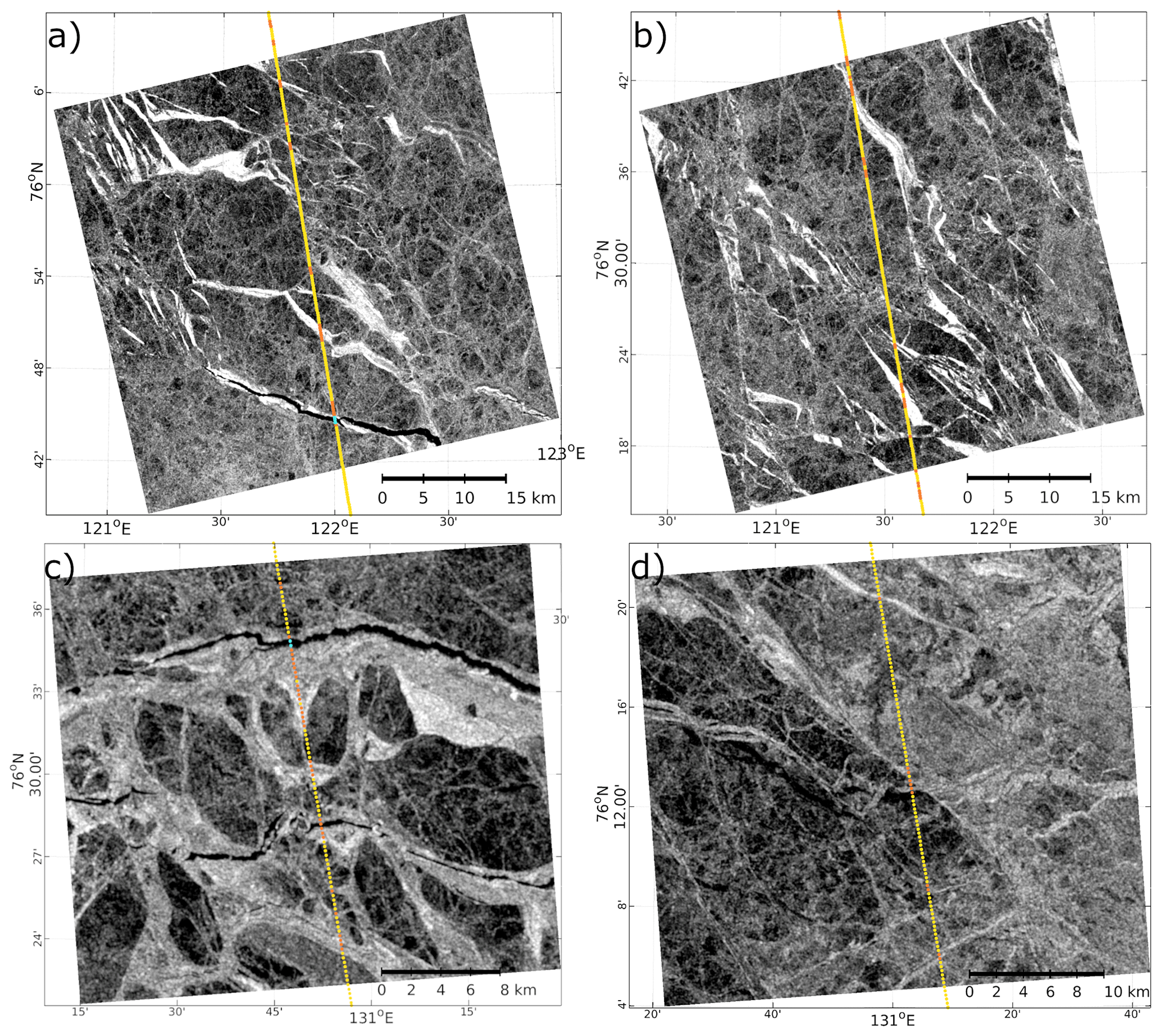
Figure 4Examples of classified CryoSat-2 observations versus HH-polarized Sentinel-1B (a, b) and Sentinel-1A (c, d) snapshots from February 2018 with acquisition time gaps of about 2 and 1 min, respectively. Orange markers show thin-ice classifications. Leads are labelled in cyan, and sea ice is in yellow. Figures are north-oriented.
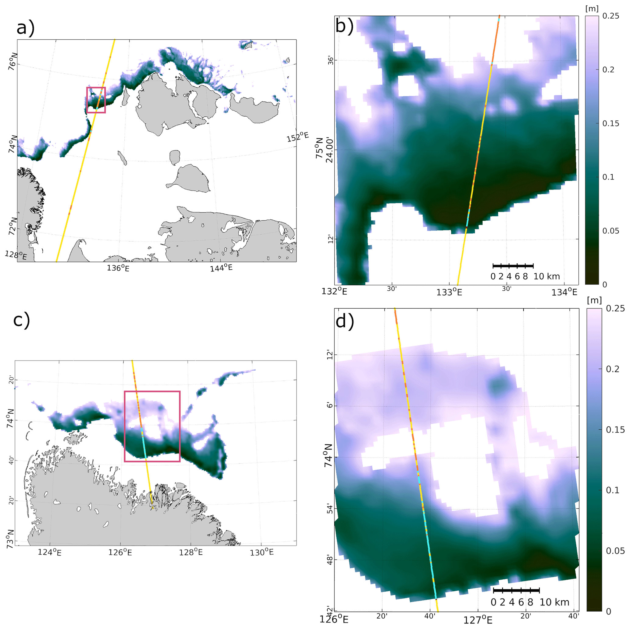
Figure 5Examples of classified CryoSat-2 observations versus MODIS TIT acquired in January 2014 (a, b) and January 2017 (c, d), respectively. The left side (a, c) shows an overview, whereas a detailed view, indicated by the purple rectangle, is given on the right side (b, d). Orange markers show thin-ice classifications. Leads are labelled in cyan, and sea ice is in yellow. Figures are north-oriented.
Figure 4 shows four subsets of two HH-polarized SAR images from February 2018 with their respective classification results from CryoSat-2 superimposed on them. Both SAR images feature at least one lead, which is recognized by the classification algorithm and highlighted by the cyan dots. Orange labels indicate thin-ice observations in the vicinity of leads and correspond to higher SAR backscatter values. Within the image, the areas appearing in light grey to almost white with their lead-like pattern represent former open-water areas that have recently frozen over. These areas of new ice can range in thickness from 10 to 30 cm (Onstott and Shuchman, 2004) and are often covered by a layer of slush (Ulander et al., 1995). The CryoSat-2 classification results agree reasonably well with the SAR images; however, not all thin-ice surfaces and leads are always correctly detected (e.g. Fig. 4c and d). Potential reasons for this are two-fold: from the SAR point of view, a complete interpretation of the SAR pixel values is not possible. From the altimetry point of view, off-nadir effects, such as when a dominant and specular lead is not in the nadir direction, may overlay clear leads or thin-ice radar echoes, which hence prevents clear identification, in particular if the lead or thin-ice surface is very small, i.e. less then 1 % of the illuminated surface (Drinkwater, 1991). These off-nadir effects can become noticeable in the waveform by the appearance of further dominant peaks in the backscatter signal, which later can lead to deviations in the height determination if a retracking algorithm specially modified for this problem is not used (see e.g. Quartly et al., 2019). Since the observations are very close together in time, differences due to ice movement or over-freezing can be excluded.
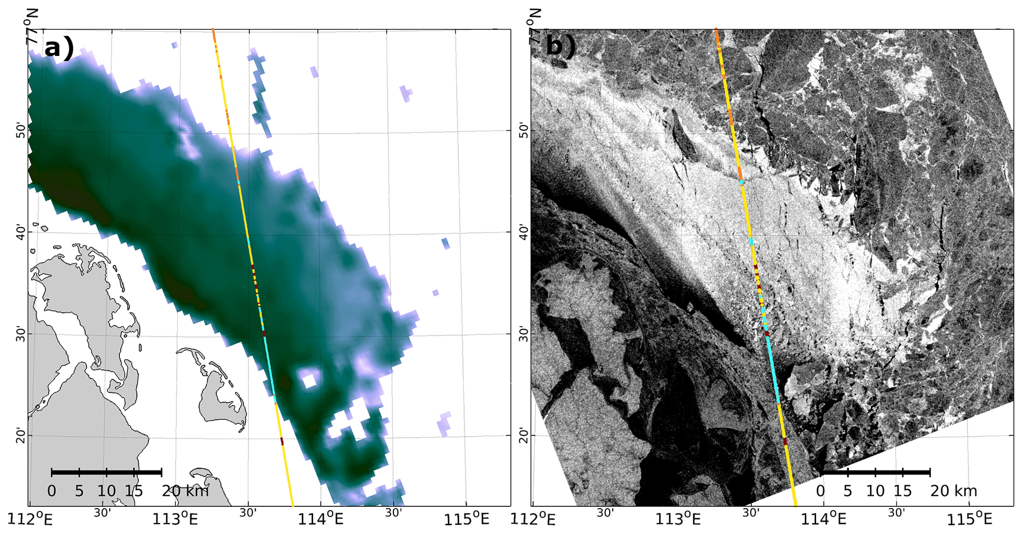
Figure 6Examples of classified CryoSat-2 observations versus MODIS TIT (a) and Sentinel-1A SAR (b) for the same location within a time gap of 7 min (MODIS) and 24 min (Sentinel-1A) with respect to CryoSat-2, respectively. Orange markers show thin-ice classifications. Leads are labelled in cyan, and sea ice is in yellow. Red dots indicate an undefined classification. Figures are north-oriented.
A visual comparison between MODIS TIT estimates and thin-ice-assigned CryoSat-2 radar echoes are provided by Fig. 5. The sets of images were recorded in January 2014 and 2017, respectively. White areas in the north indicate either a lack of data due to present cloud cover or an ice-thickness estimate above 25 cm. Towards the south, thin-ice areas are bounded by either the coast line and/or the extensive presence of landfast sea ice (Preußer et al., 2019; Selyuzhenok et al., 2015; Dmitrenko et al., 2005). Northwards, leaving the respective coastline or fast-ice edges, MODIS TIT features a rather steady increase. The respective CryoSat-2 classification generally agrees with respect to the MODIS TIT, showing primarily lead and thin-ice classifications. Qualitatively, the respective classifications appear within expectations, in particular with lead classifications close to the coastline- or fast-ice-associated ice edge in the south, where the sea ice is thinnest, and thin-ice classifications further north, where MODIS features thicker thin-ice estimates (see Fig. 5c and d). However, in most cases a direct distinction between thicker sea-ice and thin-ice areas is not possible due to the coarse pixel resolution of MODIS and the variability in ice thickness within a MODIS pixel in comparison to CryoSat-2 which leads to the fact that one MODIS TIT pixel can contain up to three CryoSat-2 observations. Nevertheless, a general connection between thin-ice-labelled radar returns in the direct vicinity of thin sea ice can be recognized. This relationship is investigated more deeply using the full MODIS database.
Figure 6 displays a CryoSat-2, MODIS, and Sentinel-1A comparison from 1 March 2018 featuring acquisition time gaps less than 17 min (more details can be found in the Appendix). This gives the very rare opportunity to analyse observations of all three sensors within a 30 min time frame. It shows the different behaviour and dependencies of optical and microwave sensors with respect to different sea-ice surfaces and their physical properties (e.g. surface roughness). The scene shows very thin ice close to the landfast-ice edge near Taymyr in the northeastern part of the Laptev Sea region (Dmitrenko et al., 2005; Selyuzhenok et al., 2015). The polynya observed by MODIS appears very bright in the SAR image and is likely caused by a high sea-ice surface roughness, potentially due to e.g. the presence of frost flowers (Hollands and Dierking, 2016; Dierking, 2013) or surface waves. In contrast to the impact this has on the side-looking SAR, the increase in diffuse surface scattering results in a wider waveform with smaller peak power for the nadir-looking CryoSat-2. We note here that this change in waveform properties can be caused by a change in roughness at the radar wavelength scale or large scales, e.g. by ice deformation. It is unlikely that larger areas covered solely by thin sheet ice have significant surface height variability or a considerable snow layer. It has been shown by Landy et al. (2020) that the increase in radar scale roughness can significantly affect CryoSat-2 waveform shape even for comparably flat surfaces when incoherent backscatter from radar scale roughness is taken into account. This effect may be so pronounced that several waveforms are assigned to the sea-ice category in an area where the SAR image indicates the presence of thin ice only. However, the low-backscatter region to the southeast (dark in the SAR image) featuring very thin ice is labelled correctly again as lead. While the CryoSat-2 unsupervised classification performs well in general, it was primarily developed to identify open water within sea-ice conditions. Hence, a clear distinction between thin and thick sea ice is not always possible due to a high variability in the surface roughness of thin ice. This comparison showcases how substantially the sea-ice surface can vary within small spatial scales but at the same time the potential and synergies for sea-ice investigations that lie within these multi-sensor collocations.
4.2 Quantitative analysis
For the quantitative analysis, a total of about 21 300 CryoSat-2 observations are compared with MODIS TIT observations in the Laptev Sea for the winter months January through March between 2011 and 2020. This corresponds to about 4 % of the theoretically available matched MODIS versus CryoSat-2 along-track observations (total circa: 540 000). The small percentage of matches used is explained by (1) the frequent presence of cloud cover in the Arctic and (2) the availability of large flaw polynya openings with corresponding thin-ice surfaces, which occur near the landfast-sea-ice edge.
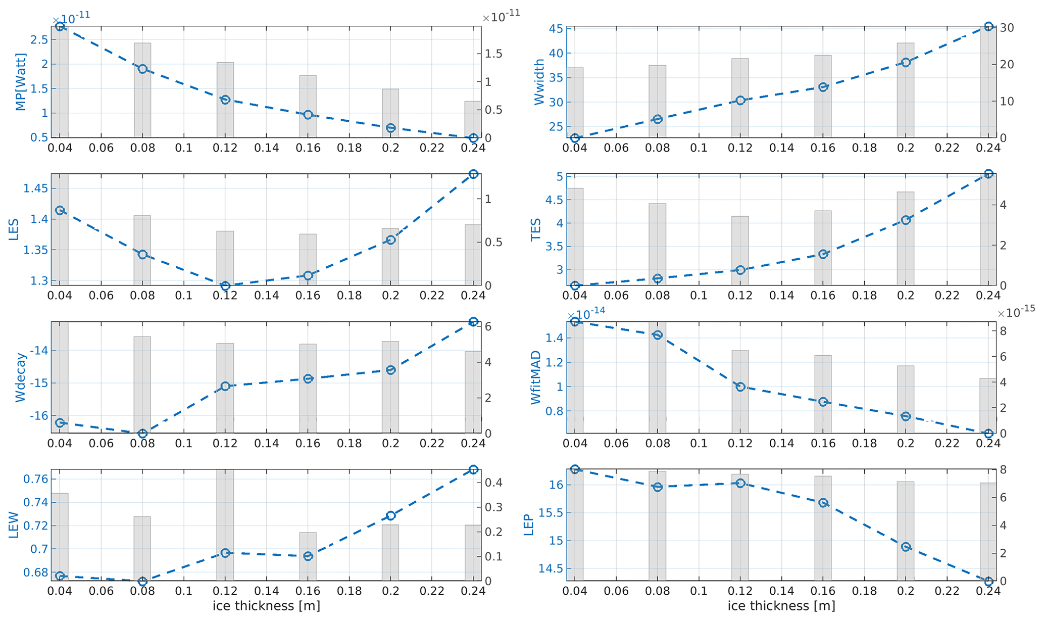
Figure 7Waveform-derived shape and power features from an unsupervised classification plus two external features of leading-edge width (LEW; Hendricks et al., 2021) and leading-edge peakiness (LEP; Ricker et al., 2014) with respect to different TIT categories. Shown are the averaged feature values (blue dotted circles) and the corresponding standard derivation (grey bar) per TIT groups of ±2 cm from 2 to 25 cm. Abbreviations of waveform features used in classification are explained in Fig. 2.
In total, 14 % of all 21 300 classifications were assigned to thin-ice surfaces and 1 % to leads. The largest proportion is attributed to thicker sea ice (85 %). With respect to valid overlaps (i.e. MODIS pixels with TIT information), about 51 % of CryoSat-2 classifications are assigned to open water and thin ice, while 45 % are assigned to other sea-ice types. Remaining waveforms are marked as undefined, e.g. due to the influence of land or instrument errors.
Besides a comparison of the CryoSat-2 classification results and the TIT from MODIS, the relationship between waveform-derived backscatter power as well as other waveform shape properties and different TIT categories is of peculiar interest. Therefore, the TIT data from MODIS are grouped into intervals of ±2 cm from 4 to 25 cm. These groups are then compared to corresponding CryoSat-2 radar waveforms, in particular, with the six waveform-derived features used in the classification and two additional waveform parameters (i.e. LEW and LEP) listed in Sect. 3.1.
Figure 7 shows the per-bin averages of the eight waveform features with their respective standard deviations indicated as grey bars in the background. The Pearson linear correlation coefficients with respect to the ice thickness are listed in the Appendix (Table A3). With the exception of LES, there is a linear (or close to linear) dependency present with respect to an increasing TIT. This is especially evident in waveform features MP, Wwidth, and TES that are intended to characterize single-peak waveforms (e.g. radar reflections by a lead). Despite a very large standard deviation in the thinner-ice class bins, an increase with rising ice thickness is a physically explainable behaviour. In general, a rougher surface corresponds to an increase in surface scattering resulting in a diminishing return back to the sensor and at the same time an increase in received off-nadir scattering by the sensor. This leads to a broadening of the received waveform as well as a drop in maximum waveform power (e.g. Drinkwater, 1991; Laxon, 1994) and, therefore, to the observed negative correlation with MP (−0.97) and the positive correlations with TES (0.94) and Wwidth (0.99). In the case of LES, which is the number of bins between the first waveform bin reaching 12.5 % and the bin of the waveform's MP (Dettmering et al., 2018), a linear relationship cannot be spotted. This might be due to a larger uncertainty associated with the first two TIT bins and their in general lower occurrence rates compared the thicker thin-ice bins or higher uncertainties in the LES processing related to very steep leading edges. Only the latter part, starting with the ±12 cm bin, features the expected behaviour. The remaining four waveform features, i.e. Wdecay, WfitMAD, LEW, and LEP, feature an apparent correlation; however, it is less clear than the ones we observed with MP, Wwidth, and TES. Similar to TES, physically one would expect a slower/smaller decay with an increase in surface roughness and therefore sea-ice thickness as well as an increase in the width of the leading edge (LEW; Landy et al., 2019) from thinner to thicker ice classes. In contrast, the LEP is expected to decrease with an increasing LEW going along with an increase in surface roughness. The median absolute deviation from the exponential fit to the waveforms is also decreasing for broader waveforms that result from additionally received backscatter from off-nadir areas due to an increased surface roughness leading to a strong negative correlation of −0.97.
Nevertheless, this comparison provides information on how different thin-ice scenarios affect the altimeter waveform. The shown dependencies between TIT and derived waveform parameters can be used e.g. to adapt and optimize altimeter waveform classifiers to thin-ice conditions and subsequently improve the sea-ice freeboard estimation in areas of frequently present thin ice.
4.3 Classification comparison
We compare the surface type classification with the CryoSat-2 surface classification described in Paul et al. (2018) to assess how thin-ice class waveforms are represented in other CryoSat-2-based products. The classification by Paul et al. (2018) was developed for the CryoSat-2 contribution to the sea-ice-thickness data record of the ESA Climate Change Initiative (Hendricks et al., 2018), hereafter named the CCI classification. The algorithm is also used in the Alfred Wegener Institute (AWI) CryoSat-2 sea-ice product v2.4 (Hendricks et al., 2021) which provides the necessary temporal coverage for this study. We use Level-2 intermediate (l2i) data, which provides the surface type flag for full-resolution orbit data for the months of October through April from November 2010 to April 2021 for the Arctic Laptev Sea regions (Fig. 1). The flags in the l2i files are based on monthly thresholds for the backscatter coefficient sigma0, the LEW, and pulse peakiness as well as supported by sea-ice concentration data (OSI-450 and OSI-430-b of the Ocean and Sea Ice Satellite Application Facility; OSI SAF, 2020) as a sea-ice mask. The surface types used in Paul et al. (2018) are comparable to this study except for the missing thin-ice class and the fact that the ocean-waveform classification solely depends on the sea-ice mask and existing land/ocean flags.
The surface type classification is based on approximately 26.5×10⁶ waveforms. The CCI classification lists 50.2 % of these in the sea-ice category, 10.9 % in the lead category, 38.7 % in the unknown category, and less then 0.1 % in the ocean category (Fig. 8a). Compared to the CCI classification, the unsupervised waveform classification algorithm (UWC) of this study has more sea-ice (79.7 %, +29.2 %) and ocean (3.9 %, +3.89 %) waveforms, as well as fewer lead type (1.9 %, −9 %) and unknown (i.e. undefined) waveforms (1.4 %, −37.3 %) in addition to the 13.0 % thin-ice waveforms (Fig. 8b). The classification matrix (Fig. 8c) shows that the UWC thin-ice waveforms are mostly distributed in CCI unknown (46.3 %) and CCI lead (53.4 %) surface types with a negligible contribution of CCI sea-ice waveforms (0.3 %). UWC lead classifications are almost exclusively (96.8 %) in the CCI lead class, showing a good agreement in the identification of open-water leads. UWC sea-ice classification not only has a good agreement with CCI sea-ice classifications (61.9 %) but also includes waveforms the CCI algorithm labels as unknown (35.6 %).
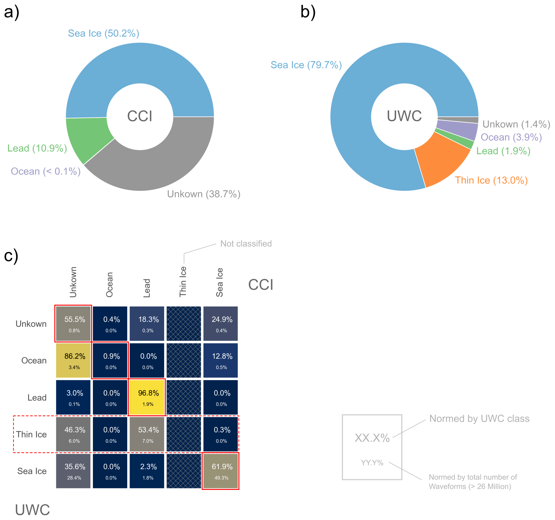
Figure 8Surface type classification statistics of CryoSat-2 data for the Arctic Laptev Sea region (Fig. 1) for the ESA Climate Change Initiative (CCI) algorithm described in Paul et al. (2018) (a), the unsupervised waveform classification (UWC) of this study (b), and the classification matrix (c). The colour coding of the classification matrix and the upper percent values describe the distribution of UWC classes within CCI classes for each class combination. The lower percent values describe the fraction of the total number of waveforms in the comparison () in class combinations. The CCI surface type classification does not contain a thin-ice class.
Between the two surface type classifications algorithms, the UWC results in far fewer unknown/undefined waveforms than the CCI algorithm and, thus, provides more usable information for sea-ice freeboard and thickness retrieval. The distinction of leads and thin ice by the UWC algorithm, which are partly seen as leads in the CCI algorithm, reduces the number of sea-surface height observations but increases their reliability. It should be noted that we define a lead here in the sense of satellite altimetry as an open-water lead, which provides a true sea-surface height observation without any bias introduced by thin-ice freeboard. The sea-ice-thickness bias introduced by using thin-ice freeboard as sea-surface height on the surrounding sea ice is of the order of the TIT itself and with a maximum of 25 cm a significant fraction of typical first-year ice thickness. The fact that the CCI algorithm labels a significant portion of the UWC thin-ice waveforms as unknown demonstrates that these were rightfully excluded from either lead or sea-ice class. The latter sea-ice class is treated as an ice surface, for which range corrections for the full climatological snow cover are applied, which would also result in range biases. The distinction between open-water lead and thin-ice classes, therefore, introduces the possibility of improving both the sea-surface height and radar freeboard retrieval.
Finally, it must be noted that the official definition of the World Meteorological Organization (WMO) for the term lead includes thin ice with a thickness of up to 30 cm (WMO, 2014). To obtain lead fractions according the WMO definition or to compare lead fractions with other remote-sensing data, the thin-ice class may be added to the open-water lead class.
In the context of an increasing number of open-water areas and sea-ice thinning, which have a major impact on the energy exchange between the atmosphere and the upper-ocean layer and on sea-ice dynamics in the Arctic Ocean (e.g. Persson and Vihma, 2017), this study investigated the thin-ice detection capabilities of CryoSat-2 through comparison of altimetry-derived thin-ice surface detections and TIT information from MODIS thermal-infrared imagery. In addition, the study benefits from spatially and temporally consistent comparisons of three different remote-sensing techniques for continuous monitoring of the Arctic Ocean.
An unsupervised waveform classification approach (Dettmering et al., 2018; Müller et al., 2017), mainly developed to identify open-water targets such as leads and polynyas within the otherwise ice-covered ocean, is adopted to distinguish thin ice from water and thicker ice. Here, waveform clusters have been assigned to be of the thin-ice type due to their resemblance to lead type CryoSat-2 waveform echoes but with less distinctness. These labelled CryoSat-2 observations are compared to thin-ice estimates up to 25 cm of thickness derived from MODIS thermal imagery (Paul et al., 2015), to Sentinel-1 SAR images, and to an external classification approach (Paul et al., 2018; Hendricks et al., 2021).
A visual comparison shows good agreement between the classified CryoSat-2 altimeter data and both the Sentinel-1A/B SAR images as well as the MODIS-derived thin-ice areas despite different spatial resolutions as well as the varying delay in acquisition times between all sensors. However, especially the interpretation of the SAR images without ground-truth validation can be challenging in thin-ice areas due to a large variety of present surface conditions ranging from smooth or slushy areas (with low-backscatter returns) to areas covered with frost flowers (with high-backscatter returns). The latter also affects the CryoSat-2 radar reflections, since higher surface roughness conditions result in a more sea-ice-like waveform shape with increased noise, higher variability, and weaker peak power as well as less peakiness. This potentially results in a sea-ice group assignment. Despite the substantial difference in spatial resolution between CryoSat-2 and MODIS, the majority of lead- and thin-ice-assigned CryoSat-2 observations are located in regions with very thin ice. In the case of SAR data, CryoSat-2 can help to bring thin-ice and lead type information to a larger scale without the need to deal with substantial amounts of data and complicated processing chains. With regards to MODIS, the CryoSat-2 thin ice and lead type can help to identify subpixel scale information from MODIS that results from spectral mixing of different surfaces within a single pixel.
A quantitative comparison of the CryoSat-2 waveform-derived shape and power features and MODIS-derived TIT shows a strong linear dependency with increasing TIT, a finding that can be exploited for directly estimating sea-ice thickness in a thickness regime where the freeboard-based approach lacks sensitivity. At a minimum it brings the opportunity to use this information for adjusting retracker algorithms, such as for example the threshold first-maximum retracker algorithm (TFMRA; Helm et al., 2014), to thin-ice conditions and to modify assumptions of snow cover in these cases. It is also feasible that the obtained information can help to develop a correction term for altimeter ranges for thin-ice waveforms based on the estimated thickness and well-known density of young sea ice for precise sea-level estimation in thin-ice leads and open-water leads alike. Moreover, to enable further Arctic climate-relevant investigations using altimetry data, the presented classification of thin ice can be extended to the entire Arctic Ocean including its peripheral seas and marginal ice zone to produce maps of altimetry-derived thin-ice coverage.
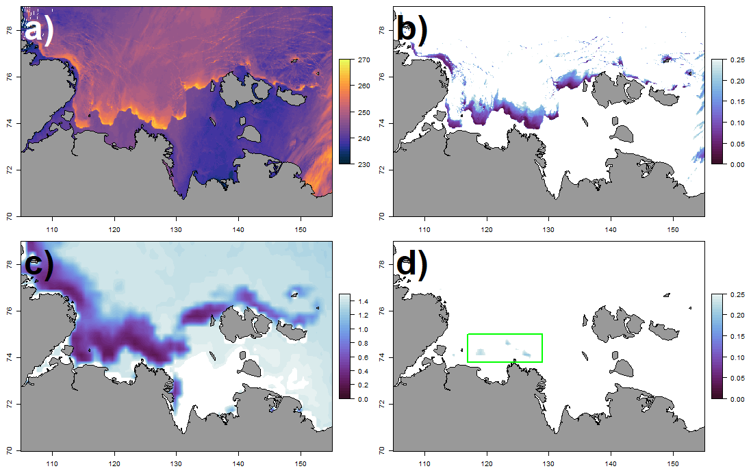
Figure A1MODIS ice-surface temperature (IST in K; a) and its associated thin-ice thickness (TIT; b) between 0 and 0.25 m and SMOS sea-ice thickness (Tian-Kunze et al., 2014) between 0 and 1.5 m (c) as well as between 0 and 0.25 m (d), respectively. A green rectangle highlights the remaining thin-ice areas in (d). Image data acquired on 5 March 2011 as shown in Fig. 3 with a different colour map.
Table A1MODIS scenes shown in Figs. 5 and 6 and record date and time difference (Δt) to CryoSat-2 observations in minutes (absolute value).
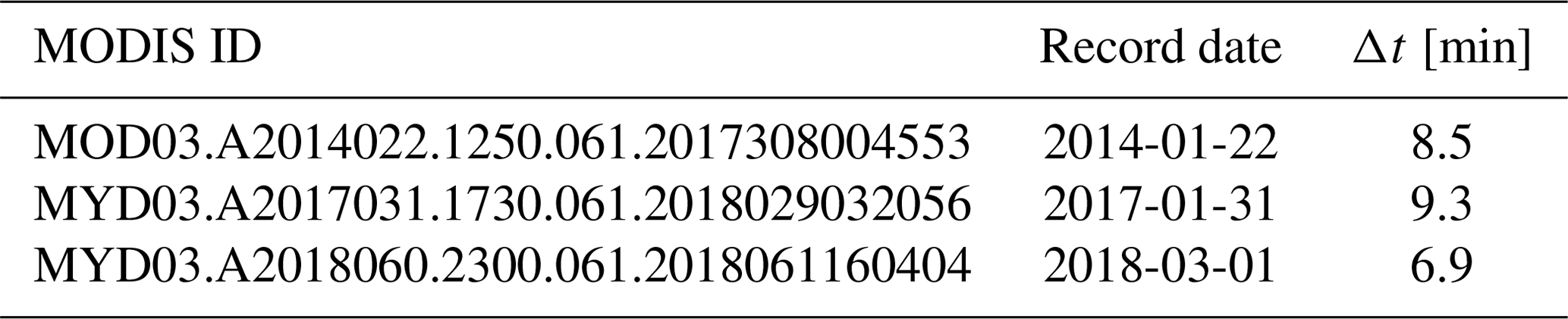
Table A2SAR images shown in Figs. 4 and 6 and record date and time difference (Δt) to CryoSat-2 observations in minutes (absolute value).

Table A3Pearson linear correlation coefficients between features and thin-ice thickness (Fig. 7). Features: maximum power (MP), waveform width (Wwidth), LES (leading-edge slope), TES (trailing-edge slope), Wdecay (Waveform decay), WfitMAD (median absolute deviation of fitted waveform), LEW (leading-edge width), and LEP (leading-edge peakiness).

CryoSat-2 L1B Baseline-D data (https://doi.org/10.5270/cr2-2cnblvi; ESA, 2019) are freely available from the CryoSat-2 science server at https://science-pds.cryosat.esa.int/#Cry0Sat2_data/Ice_Baseline_D/SIR_SAR_L1 (last access: 14 February 2023). ESA Copernicus Sentinel-1A/B Level-1 data are publicly available from the ASF DAAC (https://search.asf.alaska.edu/; ESA, 2023). MODIS Level-1B-calibrated radiances obtained from the MODIS sensors on board the polar-orbiting NASA satellites Terra (http://dx.doi.org/10.5067/MODIS/MOD021KM.061; MCST, 2017b) and Aqua (http://dx.doi.org/10.5067/MODIS/MYD021KM.061; MCST, 2017a) are freely available from the Level-1 and Atmosphere Archive and Distribution System (LAADS) Distributed Active Archive Center (DAAC) at https://ladsweb.modaps.eosdis.nasa.gov/ (last access: 14 February 2023).
The MODIS image IDs of the comparisons can be given out in a list upon request.
FLM developed the classification approach and conducted major parts of the comparison. SP designed and performed the TIT estimation from MODIS thermal-infrared imagery. FLM and SP drafted the original manuscript. SH contributed to the quantitative comparison and writing of the manuscript and supported the study with discussions and comments. DD supported the study with discussions of the applied methods and results and reviewed the manuscript.
The contact author has declared that none of the authors has any competing interests.
Publisher's note: Copernicus Publications remains neutral with regard to jurisdictional claims in published maps and institutional affiliations.
The authors want to thank the LAADS DAAC and the ASF DAAC for the provision of the MOD/MYD02 and S1-A/B data as well as the ECMWF and the CDS for the provision of the necessary ERA5 reanalysis data at no cost. Moreover, they want to thank ESA for operating and managing the Earth Explorer Opportunity Mission CryoSat-2. We thank two anonymous reviewers for their valuable comments that helped to improve the paper.
This work was supported by the Technical University of Munich (TUM) in the framework of the Open Access Publishing Program.
This paper was edited by David Schroeder and reviewed by two anonymous referees.
Adams, S., Willmes, S., Schröder, D., Heinemann, G., Bauer, M., and Krumpen, T.: Improvement and sensitivity analysis of thermal thin-ice thickness retrievals, IEEE T. Geosci. Remote, 51, 3306–3318, 2012. a
Aldenhoff, W., Heuzé, C., and Eriksson, L. E. B.: Sensitivity of Radar Altimeter Waveform to Changes in Sea Ice Type at Resolution of Synthetic Aperture Radar, Remote Sens.-Basel, 11, 2602, https://doi.org/10.3390/rs11222602, 2019. a
Alexandrov, V., Sandven, S., Wahlin, J., and Johannessen, O. M.: The relation between sea ice thickness and freeboard in the Arctic, The Cryosphere, 4, 373–380, https://doi.org/10.5194/tc-4-373-2010, 2010. a
Bouzinac, C.: CryoSat-2 Product Handbook Baseline D 1.1 C2-LI-ACS-ESL-5319, European Space Agency, https://earth.esa.int/eogateway/documents/20142/37627/CryoSat-Baseline-D-Product-Handbook.pdf (last access: October 2021), 2019. a
Celebi, M.: Partitional Clustering Algorithms, EBL-Schweitzer, Springer International Publishing, ISBN 978-3-319-09259-1, https://doi.org/10.1007/978-3-319-09259-1, 2014. a
Dettmering, D., Wynne, A., Müller, F. L., Passaro, M., and Seitz, F.: Lead Detection in Polar Oceans–A Comparison of Different Classification Methods for Cryosat-2 SAR Data, Remote Sens.-Basel, 10, 1190, https://doi.org/10.3390/rs10081190, 2018. a, b, c, d, e, f
Dierking, W.: Sea Ice Monitoring by Synthetic Aperture Radar, Oceanography, 26, 100–111, https://doi.org/10.5670/oceanog.2013.33, 2013. a, b
Dmitrenko, I. A., Tyshko, K. N., Kirillov, S. A., Eicken, H., Hölemann, J. A., and Kassens, H.: Impact of flaw polynyas on the hydrography of the Laptev Sea, Global Planet. Change, 48, 9–27, https://doi.org/10.1016/j.gloplacha.2004.12.016, 2005. a, b
Drinkwater, M. R.: Ku band airborne radar altimeter observations of marginal sea ice during the 1984 Marginal Ice Zone Experiment, J. Geophys. Res.-Oceans, 96, 4555–4572, https://doi.org/10.1029/90JC01954, 1991. a, b
Drucker, R., Martin, S., and Moritz, R.: Observations of ice thickness and frazil ice in the St. Lawrence Island polynya from satellite imagery, upward looking sonar, and salinity/temperature moorings, J. Geophys. Res.-Oceans, 108, 3149, https://doi.org/10.1029/2001JC001213, 2003. a
ESA: Cryosat L1b SAR Precise Orbit Baseline D, ESA [data set], https://doi.org/10.5270/cr2-2cnblvi, 2019. a
ESA: Copernicus Sentinel data 2018, Retrieved from ASF DAAC [2021-05-14] processed by ESA, https://search.asf.alaska.edu/, last access: 14 February 2023. a
Frey, R. A., Ackerman, S. A., Liu, Y., Strabala, K. I., Zhang, H., Key, J. R., and Wang, X.: Cloud Detection with MODIS. Part I: Improvements in the MODIS Cloud Mask for Collection 5, J. Atmos. Ocean. Tech., 25, 1057–1072, https://doi.org/10.1175/2008JTECHA1052.1, 2008. a
Guerreiro, K., Fleury, S., Zakharova, E., Kouraev, A., Rémy, F., and Maisongrande, P.: Comparison of CryoSat-2 and ENVISAT radar freeboard over Arctic sea ice: toward an improved Envisat freeboard retrieval, The Cryosphere, 11, 2059–2073, https://doi.org/10.5194/tc-11-2059-2017, 2017. a
Helm, V., Humbert, A., and Miller, H.: Elevation and elevation change of Greenland and Antarctica derived from CryoSat-2, The Cryosphere, 8, 1539–1559, https://doi.org/10.5194/tc-8-1539-2014, 2014. a
Hendricks, S., Paul, S., and Rinne, E.: ESA Sea Ice Climate Change Initiative (Sea_Ice_cci): Northern hemisphere sea ice thickness from the CryoSat-2 satellite on a monthly grid (L3C), v2.0, https://doi.org/10.5285/FF79D140824F42DD92B204B4F1E9E7C2, 2018. a
Hendricks, S., Ricker, R., and Paul, S.: Product User Guide & Algorithm Specification: AWI CryoSat-2 Sea Ice Thickness (version 2.4), https://epic.awi.de/id/eprint/54733/ (last access: 14 February 2023), 2021. a, b, c, d
Hersbach, H., Bell, B., Berrisford, P., Hirahara, S., Horányi, A., Muñoz-Sabater, J., Nicolas, J., Peubey, C., Radu, R., Schepers, D., Simmons, A., Soci, C., Abdalla, S., Abellan, X., Balsamo, G., Bechtold, P., Biavati, G., Bidlot, J., Bonavita, M., De Chiara, G., Dahlgren, P., Dee, D., Diamantakis, M., Dragani, R., Flemming, J., Forbes, R., Fuentes, M., Geer, A., Haimberger, L., Healy, S., Hogan, R. J., Hólm, E., Janisková, M., Keeley, S., Laloyaux, P., Lopez, P., Lupu, C.,Radnoti, G., de Rosnay, P., Rozum, I., Vamborg, F., Villaume, S., and Thépaut, J.-N.: The ERA5 global reanalysis, Q. J. Roy. Meteor. Soc., 146, 1999–2049, 2020. a
Hollands, T. and Dierking, W.: Dynamics of the Terra Nova Bay Polynya: The potential of multi-sensor satellite observations, Remote Sens. Environ., 187, 30–48, https://doi.org/10.1016/j.rse.2016.10.003, 2016. a, b
Huntemann, M., Heygster, G., Kaleschke, L., Krumpen, T., Mäkynen, M., and Drusch, M.: Empirical sea ice thickness retrieval during the freeze-up period from SMOS high incident angle observations, The Cryosphere, 8, 439–451, https://doi.org/10.5194/tc-8-439-2014, 2014. a, b, c
Kalnay, E., Kanamitsu, M., Kistler, R., Collins, W., Deaven, D., Gandin, L., Iredell, M., Saha, S., White, G., Woollen, J., Zhu, Y., Chelliah, M., Ebisuzaki, W., Higgins, W., Janowiak, J., Mo, K. C., Ropelewski, C., Wang, J., Leetmaa, A., Reynolds, R., Jenne, R., and Joseph, D.: The NCEP/NCAR 40-Year Reanalysis Project, B. Am. Meteorol. Soc., 77, 437–472, https://doi.org/10.1175/1520-0477(1996)077<0437:TNYRP>2.0.CO;2, 1996. a
Kurtz, N. T., Galin, N., and Studinger, M.: An improved CryoSat-2 sea ice freeboard retrieval algorithm through the use of waveform fitting, The Cryosphere, 8, 1217–1237, https://doi.org/10.5194/tc-8-1217-2014, 2014. a
Landy, J. C., Tsamados, M., and Scharien, R. K.: A Facet-Based Numerical Model for Simulating SAR Altimeter Echoes From Heterogeneous Sea Ice Surfaces, IEEE T. Geosci. Remote, 57, 4164–4180, https://doi.org/10.1109/TGRS.2018.2889763, 2019. a, b, c
Landy, J. C., Petty, A. A., Tsamados, M., and Stroeve, J. C.: Sea Ice Roughness Overlooked as a Key Source of Uncertainty in CryoSat-2 Ice Freeboard Retrievals, J. Geophys. Res.-Oceans, 125, e2019JC015820, https://doi.org/10.1029/2019JC015820, 2020. a
Laxon, S.: Sea ice altimeter processing scheme at the EODC, Int. J. Remote Sens., 15, 915–924, https://doi.org/10.1080/01431169408954124, 1994. a, b
Laxon, S., Peacock, N., and Smith, D.: High interannual variability of sea ice thickness in the Arctic region, Nature, 425, 947–950, 2003. a
Lee, S., Kim, H.-C., and Im, J.: Arctic lead detection using a waveform mixture algorithm from CryoSat-2 data, The Cryosphere, 12, 1665–1679, https://doi.org/10.5194/tc-12-1665-2018, 2018. a
Mallett, R. D. C., Lawrence, I. R., Stroeve, J. C., Landy, J. C., and Tsamados, M.: Brief communication: Conventional assumptions involving the speed of radar waves in snow introduce systematic underestimates to sea ice thickness and seasonal growth rate estimates, The Cryosphere, 14, 251–260, https://doi.org/10.5194/tc-14-251-2020, 2020. a
Maykut, G. A.: Energy exchange over young sea ice in the central Arctic, J. Geophys. Res.-Oceans, 83, 3646–3658, https://doi.org/10.1029/JC083iC07p03646, 1978. a
MCST – MODIS Characterization Support Team: MODIS 1 km Calibrated Radiances Product, NASA MODIS Adaptive Processing System, Goddard Space Flight Center [data set], http://dx.doi.org/10.5067/MODIS/MYD021KM.061, 2017a. a, b
MCST – MODIS Characterization Support Team: MODIS 1 km Calibrated Radiances Product, NASA MODIS Adaptive Processing System, Goddard Space Flight Center [data set], http://dx.doi.org/10.5067/MODIS/MOD021KM.061, 2017b. a, b
Meier, W. N., Hovelsrud, G. K., van Oort, B. E., Key, J. R., Kovacs, K. M., Michel, C., Haas, C., Granskog, M. A., Gerland, S., Perovich, D. K., Makshtas, A., and Reist, J. D.: Arctic sea ice in transformation: A review of recent observed changes and impacts on biology and human activity, Rev. Geophys., 52, 185–217, https://doi.org/10.1002/2013RG000431, 2014. a
Meloni, M., Bouffard, J., Parrinello, T., Dawson, G., Garnier, F., Helm, V., Di Bella, A., Hendricks, S., Ricker, R., Webb, E., Wright, B., Nielsen, K., Lee, S., Passaro, M., Scagliola, M., Simonsen, S. B., Sandberg Sørensen, L., Brockley, D., Baker, S., Fleury, S., Bamber, J., Maestri, L., Skourup, H., Forsberg, R., and Mizzi, L.: CryoSat Ice Baseline-D validation and evolutions, The Cryosphere, 14, 1889–1907, https://doi.org/10.5194/tc-14-1889-2020, 2020. a
Morales Maqueda, M. A., Willmott, A. J., and Biggs, N. R. T.: Polynya Dynamics: a Review of Observations and Modeling, Rev. Geophys., 42, RG1004, https://doi.org/10.1029/2002RG000116, 2004. a
Müller, F. L., Dettmering, D., Bosch, W., and Seitz, F.: Monitoring the Arctic Seas: How Satellite Altimetry Can Be Used to Detect Open Water in Sea-Ice Regions, Remote Sens.-Basel, 9, 551, https://doi.org/10.3390/rs9060551, 2017. a, b, c, d, e, f, g
Murashkin, D., Spreen, G., Huntemann, M., and Dierking, W.: Method for detection of leads from Sentinel-1 SAR images, Ann. Glaciol., 59, 124–136, https://doi.org/10.1017/aog.2018.6, 2018. a, b
Onstott, R. G. and Shuchman, R. A.: SAR Measurements of Sea Ice, in: Synthetic Aperture Radar: Marine User's Manual, edited by: Jackson, C. R. and Apel, J. R., US Department of Commerce, National Oceanic and Atmospheric Administration, National Environmental Satellite, Data, and Information Service, Office of Research and Applications, 81–115, https://www.sarusersmanual.com/ (last access: 14 February 2023), 2004. a, b
OSI SAF: Global Sea Ice Concentration Interim Climate Data Record, Release 2 – DMSP, https://doi.org/10.15770/EUM_SAF_OSI_NRT_2008, 2020. a
Park, J.-W., Korosov, A. A., Babiker, M., Won, J.-S., Hansen, M. W., and Kim, H.-C.: Classification of sea ice types in Sentinel-1 synthetic aperture radar images, The Cryosphere, 14, 2629–2645, https://doi.org/10.5194/tc-14-2629-2020, 2020. a
Passaro, M., Müller, F. L., and Dettmering, D.: Lead detection using Cryosat-2 delay-doppler processing and Sentinel-1 SAR images, Adv. Space Res., 62, 1610–1625, https://doi.org/10.1016/j.asr.2017.07.011, 2018. a, b
Passaro, M., Müller, F., and Dettmering, D.: Baltic+ SEAL: Algorithm Theoretical Baseline Document (ATBD), Version 2.1. Technical report delivered under the Baltic+ SEAL project, Tech. rep., ESA, https://doi.org/10.5270/esa.BalticSEAL.ATBDV2.1, 2020. a
Passaro, M., Müller, F. L., Oelsmann, J., Rautiainen, L., Dettmering, D., Hart-Davis, M. G., Abulaitijiang, A., Andersen, O. B., Høyer, J. L., Madsen, K. S., Ringgaard, I. M., Särkkä, J., Scarrott, R., Schwatke, C., Seitz, F., Tuomi, L., Restano, M., and Benveniste, J.: Absolute Baltic Sea Level Trends in the Satellite Altimetry Era: A Revisit, Frontiers in Marine Science, 8, 647607, https://doi.org/10.3389/fmars.2021.647607, 2021. a
Paul, S., Willmes, S., and Heinemann, G.: Long-term coastal-polynya dynamics in the southern Weddell Sea from MODIS thermal-infrared imagery, The Cryosphere, 9, 2027–2041, https://doi.org/10.5194/tc-9-2027-2015, 2015. a, b, c, d
Paul, S., Hendricks, S., Ricker, R., Kern, S., and Rinne, E.: Empirical parametrization of Envisat freeboard retrieval of Arctic and Antarctic sea ice based on CryoSat-2: progress in the ESA Climate Change Initiative, The Cryosphere, 12, 2437–2460, https://doi.org/10.5194/tc-12-2437-2018, 2018. a, b, c, d, e, f, g, h, i, j
Peacock, N. R. and Laxon, S. W.: Sea surface height determination in the Arctic Ocean from ERS altimetry, J. Geophys. Res.-Oceans, 109, C07001, https://doi.org/10.1029/2001JC001026, 2004. a, b
Persson, O. and Vihma, T.: The atmosphere over sea ice, in: Sea Ice, Chap. 6, John Wiley & Sons, Ltd, 160–196, https://doi.org/10.1002/9781118778371.ch6, 2017. a
Preußer, A., Heinemann, G., Willmes, S., and Paul, S.: Circumpolar polynya regions and ice production in the Arctic: results from MODIS thermal infrared imagery from 2002/2003 to 2014/2015 with a regional focus on the Laptev Sea, The Cryosphere, 10, 3021–3042, https://doi.org/10.5194/tc-10-3021-2016, 2016. a, b
Preußer, A., Ohshima, K. I., Iwamoto, K., Willmes, S., and Heinemann, G.: Retrieval of Wintertime Sea Ice Production in Arctic Polynyas Using Thermal Infrared and Passive Microwave Remote Sensing Data, J. Geophys. Res.-Oceans, 124, 5503–5528, https://doi.org/10.1029/2019JC014976, 2019. a, b, c, d
Quartly, G. D., Rinne, E., Passaro, M., Andersen, O. B., Dinardo, S., Fleury, S., Guillot, A., Hendricks, S., Kurekin, A. A., Müller, F. L., Ricker, R., Skourup, H., and Tsamados, M.: Retrieving Sea Level and Freeboard in the Arctic: A Review of Current Radar Altimetry Methodologies and Future Perspectives, Remote Sens.-Basel, 11, 881, https://doi.org/10.3390/rs11070881, 2019. a
Reiser, F., Willmes, S., and Heinemann, G.: A New Algorithm for Daily Sea Ice Lead Identification in the Arctic and Antarctic Winter from Thermal-Infrared Satellite Imagery, Remote Sens.-Basel, 12, 1957, https://doi.org/10.3390/rs12121957, 2020. a
Ricker, R., Hendricks, S., Helm, V., Skourup, H., and Davidson, M.: Sensitivity of CryoSat-2 Arctic sea-ice freeboard and thickness on radar-waveform interpretation, The Cryosphere, 8, 1607–1622, https://doi.org/10.5194/tc-8-1607-2014, 2014. a, b
Ricker, R., Hendricks, S., Kaleschke, L., Tian-Kunze, X., King, J., and Haas, C.: A weekly Arctic sea-ice thickness data record from merged CryoSat-2 and SMOS satellite data, The Cryosphere, 11, 1607–1623, https://doi.org/10.5194/tc-11-1607-2017, 2017. a, b
Riggs, G. A. and Hall, D. K.: MODIS sea ice products user guide to collection 6, National Snow and Ice Data Center, University of Colorado, Boulder, USA, 50 pp., https://landweb.modaps.eosdis.nasa.gov/QA_WWW/forPage/user_guide/MODISC6SeaIceproductsUserguide.pdf (last access: 14 February 2023), 2015. a
Rinne, E. and Similä, M.: Utilisation of CryoSat-2 SAR altimeter in operational ice charting, The Cryosphere, 10, 121–131, https://doi.org/10.5194/tc-10-121-2016, 2016. a
Rothrock, D. A., Yu, Y., and Maykut, G. A.: Thinning of the Arctic sea-ice cover, Geophys. Res. Lett., 26, 3469–3472, https://doi.org/10.1029/1999GL010863, 1999. a
Scagliola, M.: CryoSat Footprints (Aresys Technical Note), ESA report no. XCRY-GSEG-EOPG-TN-13-0013, Tech. rep., ESA Scientific and Technical Branch ESTEC, Noordwijk, Holland, https://earth.esa.int/eogateway/documents/20142/37627/CryoSat-Footprints-ESA-Aresys.pdf/23bccdb2-d5f2-ad92-a63a-7be504e5cf7b?version=1.0&t=1623320371977 (last access: 14 February 2023), 2013. a
Selyuzhenok, V., Krumpen, T., Mahoney, A., Janout, M., and Gerdes, R.: Seasonal and interannual variability of fast ice extent in the southeastern Laptev Sea between 1999 and 2013, J. Geophys. Res.-Oceans, 120, 7791–7806, https://doi.org/10.1002/2015JC011135, 2015. a, b
Tamura, T., Ohshima, K. I., and Nihashi, S.: Mapping of sea ice production for Antarctic coastal polynyas, Geophys. Res. Lett., 35, L07606, https://doi.org/10.1029/2007GL032903, 2008. a
Thorndike, A. S., Rothrock, D. A., Maykut, G. A., and Colony, R.: The thickness distribution of sea ice, J. Geophys. Res., 80, 4501–4513, https://doi.org/10.1029/JC080i033p04501, 1975. a
Tian-Kunze, X., Kaleschke, L., Maaß, N., Mäkynen, M., Serra, N., Drusch, M., and Krumpen, T.: SMOS-derived thin sea ice thickness: algorithm baseline, product specifications and initial verification, The Cryosphere, 8, 997–1018, https://doi.org/10.5194/tc-8-997-2014, 2014. a, b, c, d, e, f, g
Toller, G., Xu, G., Kuyper, J., Isaacman, A., and Xiong, J.: MODIS Level 1B Product User's Guide, NASA/Goddard Space Flight Center, Greenbelt, USA, 62 pp., https://mcst.gsfc.nasa.gov/sites/default/files/file_attachments/M1054E_PUG_2017_0901_V6.2.2_Terra_V6.2.1_Aqua.pdf (last accessed: 16 February 2023), 2017. a
Ulander, L. M. H., Carlström, A., and Askne, J.: Effect of frost flowers, rough saline snow and slush on the ERS-l SAR backscatter of thin Arctic sea-ice, Int. J. Remote Sens., 16, 3287–3305, https://doi.org/10.1080/01431169508954631, 1995. a, b
Wernecke, A. and Kaleschke, L.: Lead detection in Arctic sea ice from CryoSat-2: quality assessment, lead area fraction and width distribution, The Cryosphere, 9, 1955–1968, https://doi.org/10.5194/tc-9-1955-2015, 2015. a
Willmes, S. and Heinemann, G.: Pan-Arctic lead detection from MODIS thermal infrared imagery, Ann. Glaciol., 56, 29–37, 2015. a
Willmes, S. and Heinemann, G.: Sea-ice wintertime lead frequencies and regional characteristics in the Arctic, 2003–2015, Remote Sens.-Basel, 8, 4, 2016. a
Willmes, S., Krumpen, T., Adams, S., Rabenstein, L., Haas, C., Hoelemann, J., Hendricks, S., and Heinemann, G.: Cross-validation of polynya monitoring methods from multisensor satellite and airborne data: a case study for the Laptev Sea, Can. J. Remote Sens., 36, S196–S210, https://doi.org/10.5589/m10-012, 2010. a, b
Wingham, D., Fran, C., Bouzinac, C., Rostan, D. B. F., Viau, P., and Wallis, D.: CryoSat: A mission to determine the fluctuations in Earth's land and marine ice fields, Adv. Space Res., 37, 841–871, https://doi.org/10.1016/j.asr.2005.07.027, 2006. a
WMO: Sea Ice Nomenclature, https://library.wmo.int/index.php?lvl=notice_display&id=6772 (last access: 29 April 2022), 2014. a, b
Yu, Y. and Rothrock, D. A.: Thin ice thickness from satellite thermal imagery, J. Geophys. Res.-Oceans, 101, 25753–25766, https://doi.org/10.1029/96JC02242, 1996. a, b
Zygmuntowska, M., Khvorostovsky, K., Helm, V., and Sandven, S.: Waveform classification of airborne synthetic aperture radar altimeter over Arctic sea ice, The Cryosphere, 7, 1315–1324, https://doi.org/10.5194/tc-7-1315-2013, 2013. a