the Creative Commons Attribution 4.0 License.
the Creative Commons Attribution 4.0 License.
 | 22 Dec 2023
Ice floe segmentation and floe size distribution in airborne and high-resolution optical satellite images: towards an automated labelling deep learning approach
Qin Zhang
Nick Hughes
Floe size distribution (FSD) has become a parameter of great interest in observations of sea ice because of its importance in affecting climate change, marine ecosystems, and human activities in the polar ocean. A most effective way to monitor FSD in the ice-covered regions is to apply image processing techniques to airborne and satellite remote sensing data, where the segmentation of individual ice floes is a challenge in obtaining FSD from remotely sensed images. In this study, we adopt a deep learning (DL) semantic segmentation network to fast and adaptive implement the task of ice floe instance segmentation. In order to alleviate the costly and time-consuming data annotation problem of model training, classical image processing technique is applied to automatically label ice floes in local-scale marginal ice zone (MIZ). Several state-of-the-art (SoA) semantic segmentation models are then trained on the labelled MIZ dataset and further applied to additional large-scale optical Sentinel-2 images to evaluate their performance in floe instance segmentation and to determine the best model. A post-processing algorithm is also proposed in our work to refine the segmentation. Our approach has been applied to both airborne and high-resolution optical (HRO) satellite images to derive acceptable FSDs at local and global scales.
- Article
(21194 KB) - Full-text XML
- BibTeX
- EndNote


Determining the characteristics of sea ice is critical to the understanding of physical processes in the polar regions and climate change globally (Notz and SIMIP Community, 2020). Although sea ice concentration (SIC) and sea ice thickness (SIT) are widely used parameters, the size and shape distributions of individual pieces of sea ice, i.e. floes, are also important. They can help determine SIC (Nose et al., 2020), the rate of sea ice melt (Horvat and Tziperman, 2018), ocean wave propagation in the ice pack (Squire et al., 1995), and the development and maintenance of the upper ocean mixed layer (Manucharyan and Thompson, 2017). Floe size is critical for determining ice floe mass, as within an ice field it varies more than SIT. Floes also play an important role in human activities, such as maritime navigation and offshore operations in ice-covered regions (Marchenko, 2012; Mironov, 2012). Image data from various sources are rich in environmental information (e.g. sea ice types, SIC) and from which many floe parameters (e.g. floe area, parameter, shape property) can be extracted to determine a floe size distribution (FSD) (Rothrock and Thorndike, 1984).
The extraction of individual ice floes is crucial for determining FSD and other floe characteristics from images, and the separation of connected floes has always been a challenge. The existing methods for extracting individual ice floes and estimating FSD from images are mainly based on classical image processing methods. A simple approach is to define an ice–water segmentation threshold to extract floes and then apply manual edge corrections when the threshold performs poorly (Toyota et al., 2006, 2011, 2016). Watershed transform has been adopted to detach connected floes, but excessive over-segmentation is an ineluctable problem when using this method (Blunt et al., 2012; Zhang et al., 2013). Morphological operations can be used with different improvements to determine individual ice floes, but the methods operate directly on binarized floe images and thus cannot separate out the floes that have no or few gaps with any surrounding floes after binarization (Banfield, 1991; Banfield and Raftery, 1992; Soh et al., 1998; Steer et al., 2008; Wang et al., 2016). The gradient vector flow (GVF) snake was used by Zhang and Skjetne (2015) for detecting weak floe boundaries and has achieved excellent results in segmenting individual floes from marginal ice zone (MIZ) images, in which a large number of floes are connected to each other. However, this method is not time-effective and may not work well with floe images other than MIZ images, especially the larger-scale images such as satellite imagery (Zhang, 2020; Zhang and Skjetne, 2018). These classical image-processing-based methods suffer from segmentation problems and are more or less limited by the need for manual intervention in processing individual images. Due to the vast volumes of image data now being collected by Earth observation programmes such as Copernicus, so-called “big data”, manual intervention is undesirable due to its inefficiency. Autonomous, trustworthy, and time-efficient methods thus need to be developed.
Deep learning (DL) methods have nowadays proven to deliver superior accuracy in a wide range of image processing applications. Pixel-based DL methods are able to map complex features at the pixel level from an image in an automated process, and they have also been applied in extracting all ice pixels from images consisting of a mixture of sea ice and water (Khaleghian et al., 2021; Gonçalves and Lynch, 2021; Zhang et al., 2021). However, most of these studies grouped the pixels belonging to different ice regions or floes into the same class (i.e. the class of ice) and did not contribute to the identification of individual ice floes, which is an instance segmentation problem that requires multiple ice floes to be treated as distinct individual instances. Few studies have employed DL methods to identify individual ice floes. A semantic segmentation model, ResUNet, was used in Nagi et al. (2021) to segment individual floes that were far apart from each other and then used ConvCRF to refine the segmentation results. This method, however, simply divided an image into two classes of ice and background and was unable to separate connected floes. Cai et al. (2022) have adopted and compared two state-of-the-art (SoA) DL instance segmentation models, Mask R-CNN (He et al., 2017) and YOLACT (Bolya et al., 2019), for identifying individual model floes in an indoor ice tank. Because these models rely heavily on their own object detectors to produce instance segmentation results, neither model could fully detect every floe that appeared in the image, resulting in the loss of floes, and the segmentation accuracy was usually not high.
Training a DL model requires a sufficiently annotated dataset. However, data labelling usually involves a lot of manual work and is expensive and time-consuming, which limits the application of DL methods to extracting individual ice floes (Jing and Tian, 2021; Zhou, 2017; Chai et al., 2020). In order to minimize the manual labelling effort required from the domain experts, we use a classical image processing method to enable a manual-label free annotation of the dataset and automatically generate pseudo ground truth. We then apply DL semantic segmentation method, which assigns every pixel in an image to defined classes, to address the floe instance segmentation problem, and propose a post-processing algorithm to refine the model outputs. The application of our approach to derive FSDs from local-scale airborne imagery and global-scale satellite imagery demonstrates the effectiveness of our approach.
2.1 Image data
2.1.1 Local-scale airborne data
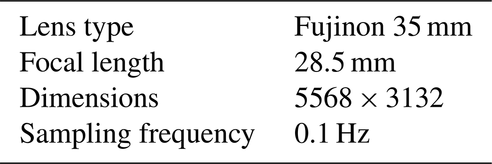
The local-scale image data are the only data we used to train DL models, and they are marginal ice zone (MIZ) images mainly from the Oden Arctic Technology Research Cruise 2015 (OATRC'15) expedition. OATRC'15 was conducted by the Norwegian University of Science and Technology (NTNU) in collaboration with the Swedish Polar Research Secretariat (SPRS) in September 2015 (Lubbad et al., 2018). Two icebreakers, Oden and Frej, were employed during this research cruise into the Arctic Ocean north of Svalbard. Among many research activities, a helicopter flight mission was accomplished when Oden was transiting in the MIZ during which an optical camera was mounted on the helicopter, as seen in Fig. 1. This enabled the acquisition of 254 high-resolution images of sea ice, of which 52 images covering MIZ regions and less blurred by water vapour were selected for this study. The resolution of the collected sea ice images depends on helicopter's flight altitude and was estimated as 0.22 m on average. The specifications of the camera can be found in Table 1 (Zhang and Skjetne, 2018).
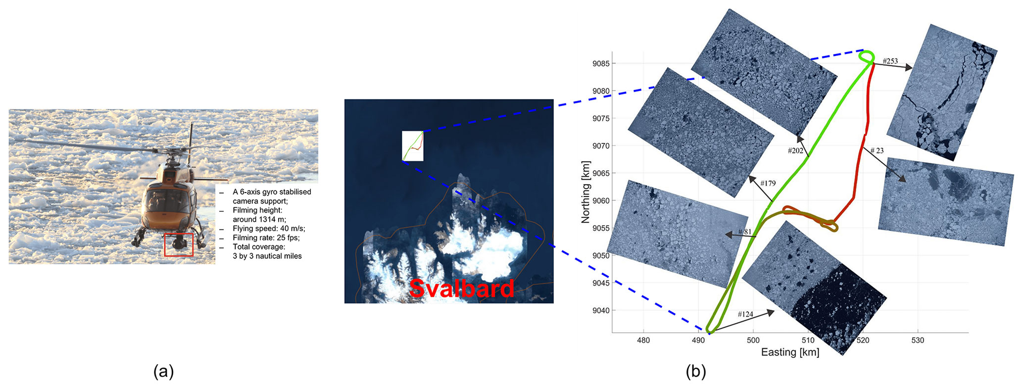
Figure 1Helicopter flight mission. (a) Helicopter showing location of the camera system. (b) Helicopter's flying route, starting from red and gradually changing into green. Source: Lubbad et al. (2018).
In addition to the MIZ images from OATRC'15, we also used another three airborne images obtained from the remote sensing UAV mission over the MIZ performed by the Northern Research Institute (NORUT) at Ny-Ålesund, Svalbard ( N E), in early May 2011. The details of this UAV mission and the specifications of the collected image data can be found in Zhang et al. (2012). For convenience, in this article, we refer to the local-scale airborne MIZ images as MIZ images.
2.1.2 Global-scale satellite data
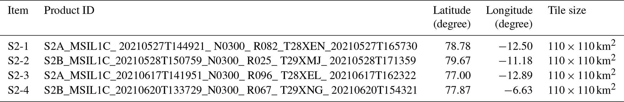
The global-scale high-resolution optical (HRO) satellite imagery data are additional test data only used to investigate the generalization ability of the DL models which were trained only on local-scale MIZ images. The S2 images are freely available from the Sentinel-2 mission of the European Copernicus programme (Copernicus Open Access Hub, 2023). The two Sentinel-2 satellites carry a multispectral instrument (MSI) that provides images consisting of 13 spectral bands: 4 bands at 10 m resolution covering visible and near-infrared (VNIR) frequencies, 6 at 20 m covering red edge and short-wave infrared (SWIR), and 3 at 60 m for atmospheric correction (Drusch et al., 2012). Figure 2 displays the locations of the four S2 Level-1 images that were acquired over the Belgica Bank area offshore of northeastern Greenland during May and June 2021, and in this article we refer to them as S2-1, S2-2, S2-3, and S2-4. Table 2 lists and identifies the filenames used, e.g. the filename of S2-1 image identifies a Level-1C product acquired by Sentinel-2A on 27 May 2021 at 14:49:21 that was acquired over tile 28XEN during relative orbit 082, and processed with the Payload Data Ground Segment (PDGS) processing baseline 03.00. More details for each S2 image can be found by searching for their product IDs on the Copernicus Open Access Hub (https://sentinels.copernicus.eu/web/sentinel/user-guides/sentinel-2-msi/naming-convention, last access: 20 December 2023).
Further examples as NetCDF files containing both gridded and vector polygon data can be downloaded from https://thredds.met.no/thredds/catalog/digitalseaice/catalog.html (last access: 20 December 2023), with a GeoJSON catalogue for these at https://bit.ly/s2floemaps (last access: 20 December 2023).
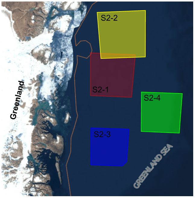
Figure 2Location map of the four Sentinel-2 image data: S2-1 in red, S2-2 in yellow, S2-3 in blue, and S2-4 in green. The map was reproduced from the Copernicus Open Access Hub, and details for each S2 image can be found on the Copernicus Open Access Hub by searching for their product IDs listed in Table 2.
2.2 Software and hardware
The platform for implementing DL models was TensorFlow 2.4.0, and the training was performed on an NVIDIA Tesla P100-PCIE GPU with 12 GB of memory. All the testing and performance comparisons of DL models, as well as the classical image processing method, for the sake of fairness, were conducted using Intel(R) Core(TM) i7-4600U CPU at 2.10 GHz, 16 GB RAM, Integrated Graphics Card, as the GPU cannot significantly reduce the execution time of the classical image processing method.
This section introduces methods and DL model we will use in ice floe segmentation. The detailed implementation process of these methods will be introduced in Sect. 4.
3.1 Training data preparation
By studying various floe images, we find that the intensities of the boundary pixels between two adjacent floes are usually significantly higher than those of water pixels and close to ice pixel intensities (Toyota et al., 2006; Denton and Timmermans, 2022). If we consider only two classes in floe segmentation, i.e. ice floe and water, and categorize floe boundary pixels into the class of water, the gap between the two classes will be narrow, and the boundary pixels between two adjacent floes will most likely be classified as ice pixels, with the result that the adjacent floes connect to each other. Therefore, we add an additional class of floe boundary, turning the two-class segmentation task into a three-class segmentation problem. In this way, the discriminative ability of the network for segmenting individual ice floes will be improved, not only by broadening the gap between the classes of ice and water but also through the learning of shape and spatial relationships between ice floes and their boundaries.
We also notice that the number of pixels belonging to the floe boundary class might be relatively small, compared to those belonging to the other two classes. Floe boundary is a hard-to-train class with pixel intensities similar to those of ice floes. It is therefore necessary to increase the proportion of floe boundary in the training dataset to balance the classes. MIZ images often contain large numbers of small ice floes crowded together, and the proportions of floe boundary pixels in the MIZ images are usually higher than that of other floe images. Using MIZ images as the training dataset is therefore beneficial to reduce the risk of class imbalance in the dataset. For this reason, we use MIZ images and their annotations to train DL models for floe instance segmentation.
3.1.1 Automated data annotation
Manually labelling ice floes in MIZ images is labour intensive, and a large effort is required to achieve automatic labelling. Because the GVF snake-based method has a superior ability of segmenting large number of small and crowded floes in MIZ images, it is thus utilized as an “annotation tool” to help automatically label individual ice floes in MIZ images. This method first uses the distance map and regional maxima of the binarized MIZ image to automatically locate the initial contours, each of which is a starting set of snake points for the evolutions. Then the GVF snake is run on each initial contour to find floe boundaries. Finally, superimposing all the detected boundaries over the binarized MIZ image, the connected floes are separated and individual floes are determined (Zhang, 2020; Zhang and Skjetne, 2018).
The output of the GVF snake-based method is a binary image with two classes: ice floe and water, as seen in Fig. 3b. Additional floe boundary class is added by tracing the contours of each segmented ice floes. To enhance floe boundaries and mitigate the imbalance of classes that may still be latent in the training dataset, we widen floe boundaries from 1 pixel to 2 pixels (i.e. inner floe boundary, which consists of pixels from the floe itself, and outer floe boundary, which mainly consists of pixels from ambiguous edges between the floe and another floe or water) in the labels. And with the help of the double-thick boundary labels, the network would be able to capture floe boundaries more accurately.
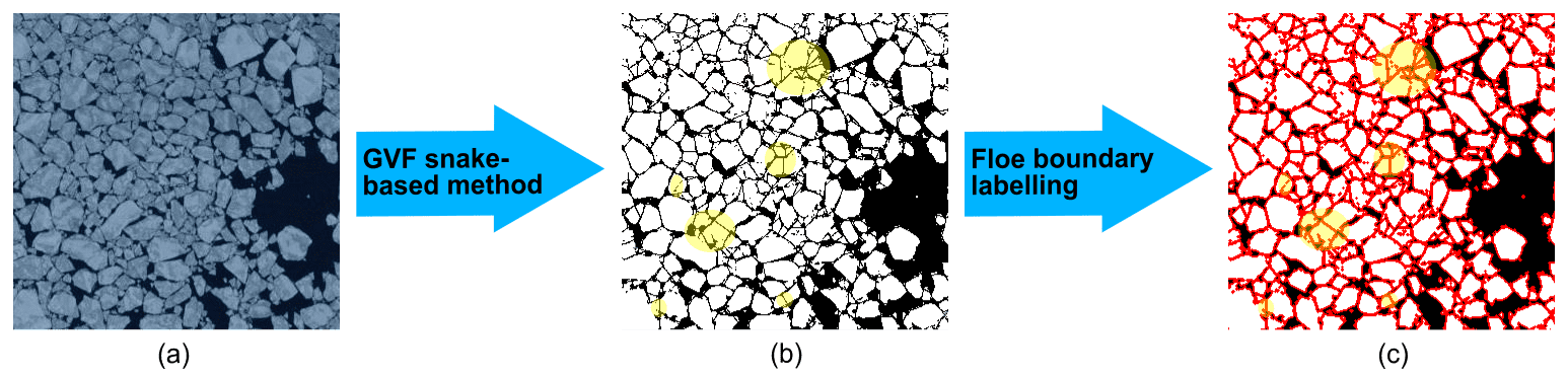
Figure 3Ice floe image annotation. (a) A small MIZ image sample; (b) floe segmentation of (a) by the GVF snake-based method; (c) three-class label annotation, produced by adding an additional floe boundary class to (b). Labels: white – ice floe; red – floe boundaries; black – water. Note that the labels annotated by the GVF snake-based method are not always accurate, as seen by the highlighted yellow regions in (b) and (c) for instance. Our approach can thus be thought of as self-supervised and weakly supervised learning that the model will learn from the inaccurate labels created from the data itself without human annotation.
3.1.2 Multi-scale division
Our MIZ images are of different sizes. Although the fully convolutional network (FCN) architectures (Long et al., 2015) can be designed for variable-size inputs (Long et al., 2015), in order to reduce memory usage and improve training efficiency, it is more practical to fix the input size of a network to a small value during the training process. Therefore, each of the images, together with the corresponding annotation, is divided into several equal-sized patches that are as close as possible to the fixed input size of the network for training.
Due to the nature of the MIZ in this example, most floes in our training image data have similar sizes and shapes. But in more general cases, floe sizes and shapes can vary greatly in an image. Small floes are typically more challenging to segment, not only because of low resolution and small size, but also due to the lack of representation of small objects in training data (Kisantal et al., 2019). To overcome this issue, we select a few floe images and divide each of these images (and also their annotations) randomly into, taking Fig. 4 as an example, 1×1, 1×2, 2×3, 3×4, and 4×5 sub-images. Note that some sub-images (e.g, 4×5 sub-images in Fig. 4) may duplicate with the patches. These duplicate sub-images should be removed so that the remaining sub-images, which we refer to as “multi-scale sub-images”, and patches appear only once in the dataset, thus preventing data leakage during the training. After automatically removing the sub-images that are duplicated with the patches by, for example, using a naming convention to overwrite the duplicated ones, the resulting multi-scale sub-images together with the patches constitute our dataset, and they will further be rescaled into the small size required by the network for training. In this way, an ice floe can be resized into several smaller ones of different scales. Thus, our multi-scale division is a data augmentation that expands the size of the training dataset and increases the diversity of floe size/shape and the appearance rate of small floes in the training dataset, and thereby helping the network improve the segmentation of small floes.
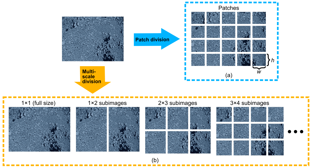
Figure 4Flowchart of the patch and multi-scale divisions. An ice floe image is divided into (a) equal-sized patches with sizes close to network's fixed input size for training and (b) random sub-images (1×1, 1×2, 2×3, 3×4, 4×5, … sub-images in this example), and the sub-images that duplicate with the patches are removed. We refer to the remaining sub-images as multi-scale sub-images.
3.2 Deep learning model
The extraction of individual ice floes is an instance segmentation problem that treats multiple floes as distinct individual instances. SoA DL instance segmentation models, such as Mask R-CNN (He et al., 2017) and YOLACT (Bolya et al., 2019), are often the intuitive choices to solve the floe instance segmentation problem. Unfortunately, these instance segmentation models are unable to completely detect all the floes in regions of high SIC where a large number of variable-sized floes touch each other (Cai et al., 2022). This results in the loss of floes and ice pixels that reduces the accuracy of FSD estimation and further leads to underestimation of SIC. An additional method or model is thus needed to determine all sea ice pixels. The encoder–decoder network architectures (Badrinarayanan et al., 2017; Ronneberger et al., 2015), which are designed for semantic image segmentation tasks, assign every pixel in an image to defined classes. They are able to extract all sea ice pixels from an image consisting of a mixture of sea ice and water and have the potential to detect individual floes by identifying floe boundaries. Therefore, a semantic segmentation approach is used in our work to address the floe instance segmentation problem.
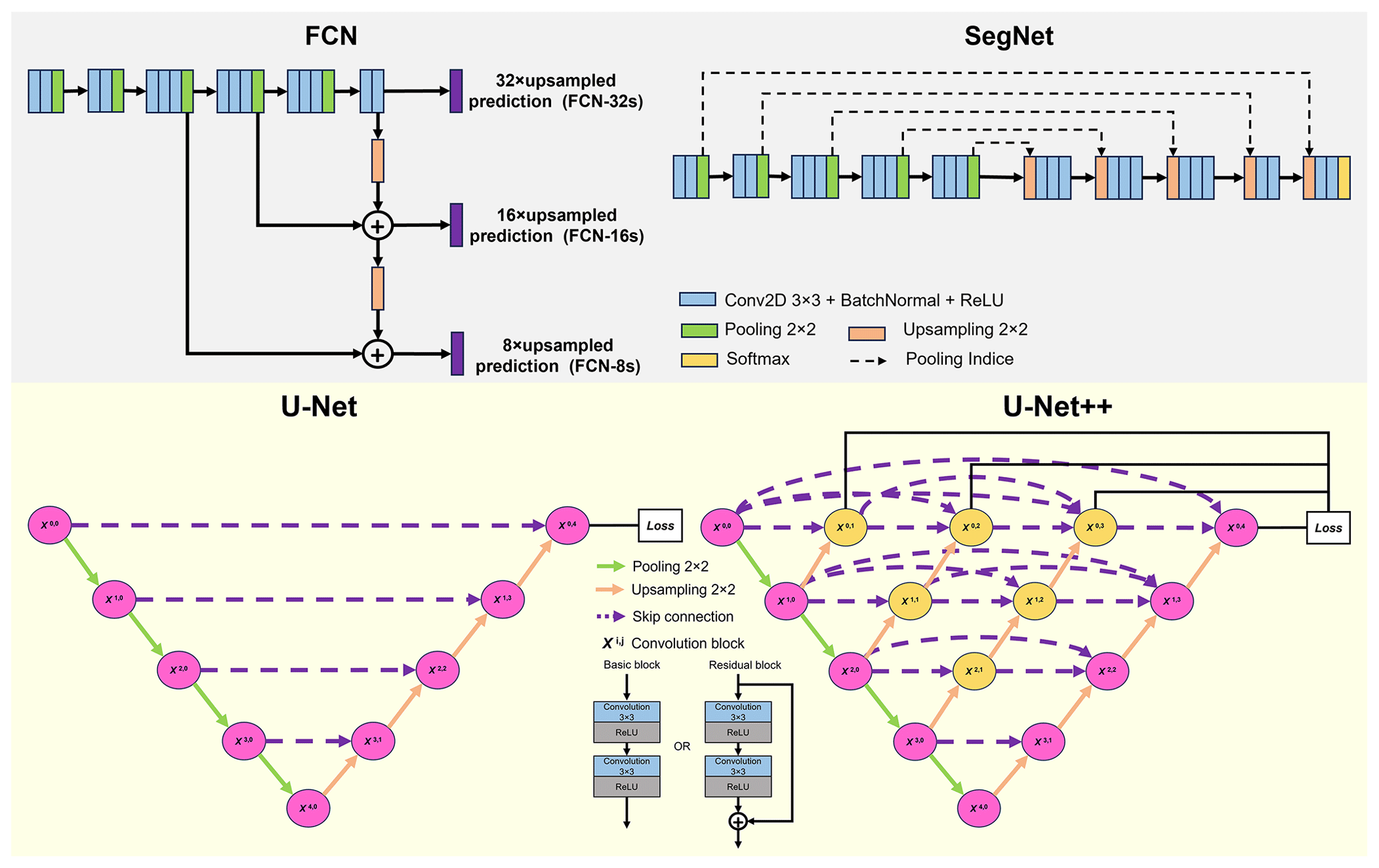
U-Net and its developments are popular DL models for semantic segmentation (Ronneberger et al., 2015; Kamrul Hasan and Linte, 2019; Zhou et al., 2018). They have achieved great success in many image segmentation applications, even with a limited training dataset (Kamrul Hasan and Linte, 2019; Zhang et al., 2018; Jeppesen et al., 2019). The basic architecture of U-Net family is a symmetric FCN encoder–decoder structure with additional skip connections. The encoder network consists of convolution blocks followed by a max-pooling downsampling to encode the input image into feature maps at multiple different levels, while the decoder network consists of upsampling followed by regular convolution operations to restore the spatial resolution of the feature maps. The skip connections use concatenation to simply combine the low-level features, extracted from the encoder, with the high-level features, obtained from the decoder, to recover the spatial information lost during the max-pooling operation. However, no solid guarantee that the same-scale feature maps from the encoder and decoder networks are the best match for fusion.
Unlike the skip connections designed in the original U-Net architecture, U-Net++ (Zhou et al., 2018), which is a variant of original U-Net, uses a series of nested dense convolutional blocks (Huang et al., 2017) on the skip pathways to bridge the semantic gap between encoder and decoder feature maps prior to fusion, and improves gradient flow in the network. Moreover, U-Net++ has deep supervision that allows us to use only one loss layer to determine the optimal depth of the network (Zhou et al., 2018, 2020).
We have conducted experiments to compare the performance of U-Net++ with other SoA models such as the family of FCNs (Long et al., 2015), SegNet (Badrinarayanan et al., 2017), U-Net, etc. in floe instance segmentation. The architecture of each model and comparisons between them can be found in Sect. 5.1. Our experimental results show that U-Net++ performs best in extracting individual ice floes even if a large number of variable-sized floes touch each other. Therefore, we employ U-Net++ in our work for the instance segmentation of ice floes.
It should be noted that the U-Net++ model is our suggestion for ice floe instance segmentation after studying different SoA DL models on the currently limited training datasets. As training datasets become richer, more robust floe segmentation models will be developed.
3.3 Post-processing
Inevitably, a few connected floes may still not be separated, and some pixels inside a segmented floe may also be misclassified as edge or water by the DL model, as seen in Fig. 6b. A post-processing is thus necessary to refine the segmentation made by DL models.
To find potential connected floes/regions, we first calculate the solidities of each segmented floe/region, given by
where f is a segmented ice floe/region, Filled(f) is the region of f with all the holes filled in, ConvexHull(f) is the smallest convex polygon that encloses the region of f, and Area[⋅] denotes the area (number of pixels) of the region. The solidity of any segmented floe/region is the ratio of its hole-filled area to its convex hull's area; it reflects the convexity of each segmented floe/region.
An under-segmented region normally has low convexity. That means that a segmented region with low solidity (i.e. the solidity is less than a cut-off threshold Ts) and large area (i.e. the area is larger than a cut-off threshold Ta) is more likely to be composed of connected ice floes. Therefore, we perform the morphological opening (which removes small protrusions and breaks the tenuous connections between objects) to those potentially under-segmented regions to detach the floes that are possibly connected. After that, we perform the morphological closing (which fills long thin channels in the interior or at the boundaries of the object) and hole filling to large-area ice floes (i.e. the floes whose area is larger than a threshold ), one by one, in order of increasing size.
The procedure of our post-processing algorithm is illustrated in Fig. 5, and Fig. 6 presents the post-processing result of an ice floe image segmentation. Note that a small number of pixels may be turned to other classes after post-processing. In particular, some isolated ice pixels or tiny floes may vanish during the opening or closing process. To avoid the loss of ice pixels and the underestimation of SIC, the vanished ice pixels are recorded and labelled as boundary pixels in our post-processing algorithm.
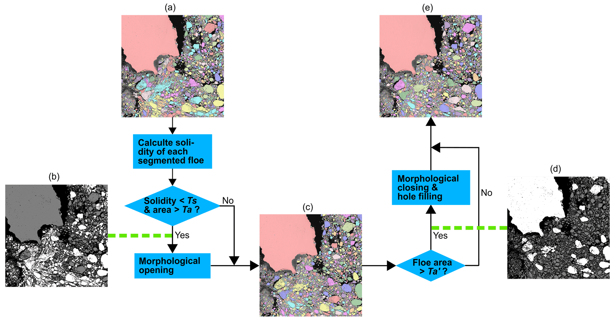
Figure 5Flowchart of the post-processing procedure. (a) Preliminary floe segmentation made by U-Net++. (b) Potential under-segmented ice floes (highlighted in white), obtained by finding the floes whose solidities are lower than a cut-off threshold Ts (which is 0.85 in our case) and areas are larger than a cut-off threshold Ta. (c) Floe segmentation after performing morphological opening on the floes found in (b). The under-segmented floes are detached. (d) Finding out the floes in (c) whose areas are larger than a threshold (highlighted in white). (e) Final post-processing result by performing morphological closing and hole filling to the ice floes in (d) one by one in order of increasing size. The segmented floes/regions in (a), (c), and (d) are labelled in different colours. Note that, only ice floes, without any floe boundaries, are presented in this figure.
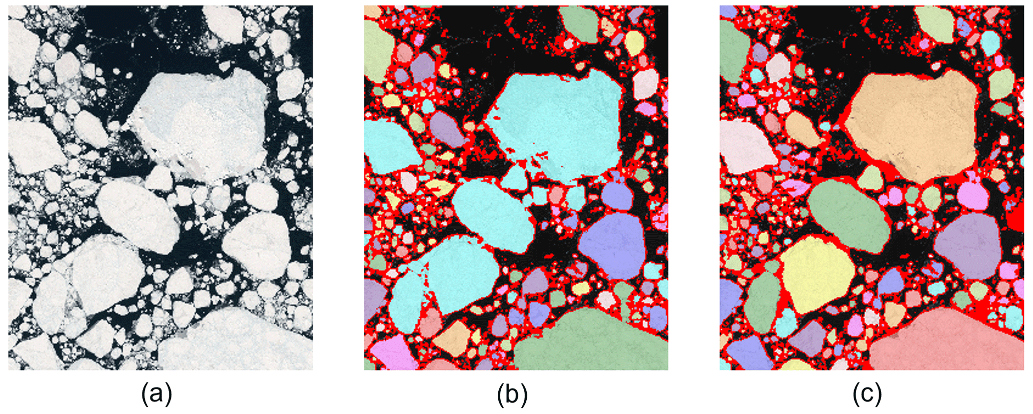
Figure 6A post-processing example. (a) A small subset of S2-1 image. (b) Preliminary segmentation of (a) by U-Net++. Some floes are still touching, and some pixel inside a floe are misclassified as edge pixels. (c) Final segmentation after performing post-processing to (b). The detected individual ice floes are labelled in different colours, and the detected floe edges are plotted in dark red.
The implementation of the our proposed approach is divided into two parts: DL model training and ice floe image processing using the trained DL model, in which the methods introduced in Sect. 3 will be applied.
4.1 DL model training
Our MIZ images were fed into the GVF snake-based method to “label” individual ice floes and floe boundaries. The entire image processing was fully automatic, using the default parameters in the GVF snake-based method (Zhang, 2018) without any manual tuning. This means that our approach can be thought of as a self-supervised learning, with the supervisory labels being created from the data itself without human annotation (Jing and Tian, 2021).
The processed image pairs, i.e. MIZ images and their annotations, were then divided into the patches with the sizes close to the fixed input size of the network for training, which was 256 × 256 pixels in our case, a restriction of the number of MIZ images and GPU memory. Some patch pairs may have severely wrong annotations1, and it is necessary to remove them from the patch dataset to minimize mislabelling in the training dataset. Owing to the characteristics of MIZ ice floes (i.e. the shapes and sizes of MIZ floes do not vary much), this can be done automatically by adopting the criteria for finding under-segmented floes introduced in the post-processing step. That is, if the ratio of the total area of the labelled floes that do not satisfy the criteria to the total area of all the labelled floes is larger than a threshold, the annotated pair will be removed. We also chose a few well-processed image pairs and divided each of them into several multi-scale sub-images, which were the sub-images that did not duplicate with the patches. These patches (333 pairs) and multi-scale sub-images (46 pairs), a total of 379 pairs of images and the corresponding annotations, constituted the final dataset we needed for training a model. And the proportions of each class in the dataset are 41.63 % ice floe, 39.83 % floe boundaries, and 18.54 % water.
After randomly splitting the dataset into training (290 pairs), validation (52 pairs), and test (37 pairs) sets, the training and validation datasets were further resized to match the training input size of the network. To increase the number of training data, data augmentation, including Gaussian blur, rotate, shift, flip, zoom, etc., was also employed in the training. The procedure of our training process is illustrated in Fig. 7.
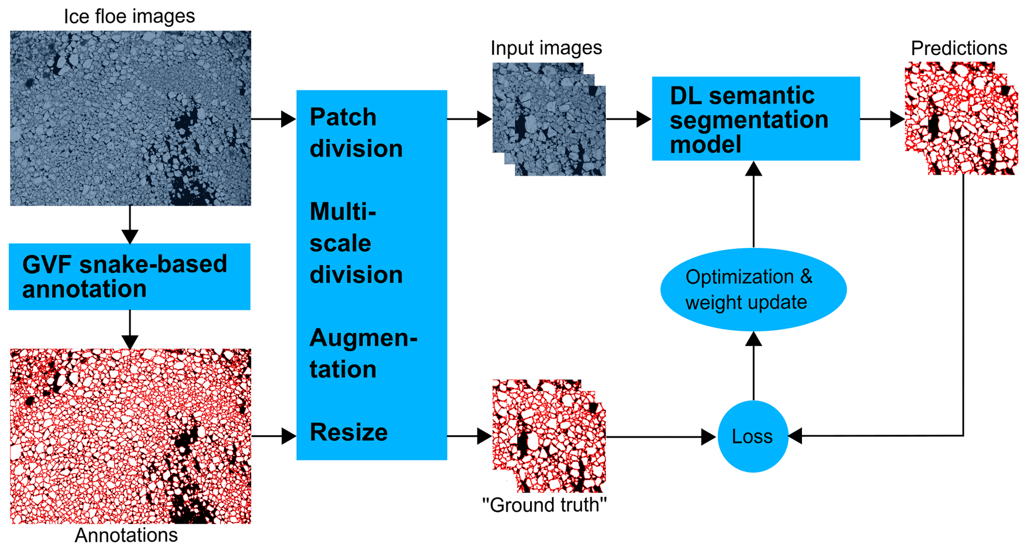
Figure 7Flowchart of the overall training procedure. Labels in the annotation: white – ice floe; red – floe boundaries; black – water.
It should be noted that our dataset still has some minor errors; i.e. some labelled ice floes are under- or over-segmented (e.g. the highlighted yellow regions in Fig. 3). These errors may reduce the robustness of the trained model. However, we kept the minor erroneous segmentations in our training dataset, leaving the issue to be further overcome by the DL network, as DL network learns the most significant features from the dataset, being able to identify small errors as outliers during the training. Therefore, our approach can also be thought of as weakly supervised learning that the model will learn from the inaccurate labels (Zhou, 2017). But for evaluating and comparing different DL models, we have manually corrected the errors in our test dataset.
The DL model was trained with a batch size of four, and an Adam optimizer was applied in the training. The learning rate was set to 10−4 for the first 50 epochs and then to 10−5 for the next 30 epochs. Note that the proportion of floe boundaries in our dataset is close to that of ice floes, while the proportion of water is a bit smaller than that of the other two classes. The smaller proportion of water has little effect on the model learning to classify water pixels, since water is an easy-to-train class with significantly lower pixel intensities than the other two classes. Therefore, there is no need to modify the loss function, and categorical cross-entropy was chosen as the loss in the training.
4.2 Ice floe image processing
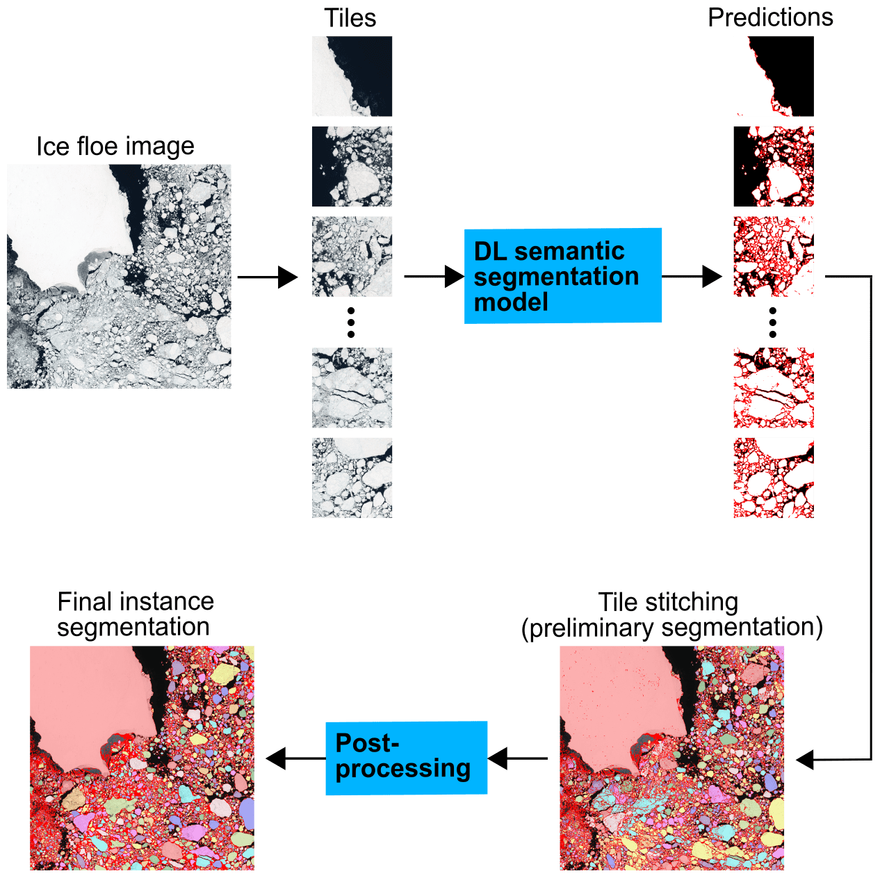
Due to the limitation of computer performance, a large image was first divided into several small tiles. Each tile was then fed to the trained model to obtain its predicted mask. Thereafter, all the predicted masks were stitched together to restore the spatial pattern, resulting in the preliminary floe instance segmentation. After post-processing the preliminary segmentation, we obtained the final floe instance segmentation. Figure 8 illustrates the workflow of the inference using the S2-1 image as an example.
This section presents the performance evaluation and comparison using different methods/hypotheses on local airborne and global satellite sea ice floe images.
5.1 DL model evaluation
We have conducted experiments to compare the performance of different SoA semantic segmentation architectures: the family of FCNs (i.e. FCN-8s, FCN-16s, FCN-32s) (Long et al., 2015), SegNet (Badrinarayanan et al., 2017), U-Net (Ronneberger et al., 2015), residual U-Net (ResUNet) (Zhang et al., 2018), and U-Net++ and residual U-Net++ (ResUNet++) (Jha et al., 2019), where the optimal depths of U-Net, ResUNet, U-Net++, and ResUNet++ are 5, 5, 5, and 6, respectively. Diagrams for each DL model can be found in Fig. 9
5.1.1 Evaluation metrics
To assess DL model performance, we use accuracy, F1 score (Goutte and Gaussier, 2005), and mean intersection of union mIoU (Long et al., 2015) as evaluation metrics:
where TP, TN, FP, and FN are pixel-wise true positive, true negative, false positive, and false negative, respectively, C is the number of classes, and IoUc is the intersection of union for class c.
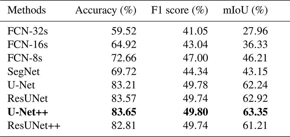
Table 3 lists the evaluation and comparison results based on our test dataset. We can see that the performance indicators of U-Net, ResUNet, U-Net++, and ResUNet++ are similar to each other and are significantly higher than those of FCN family models and SegNet, while the U-Net++ model gives a slight advantage with the highest scores on our test dataset.
Table 3Model performance indicators. The method of best performance is highlighted in bold.
5.1.2 Segmentation visualization
To further investigate the effectiveness of the models, Figs. 10 and 11 visualize the floe instance segmentation results on local-scale airborne and global-scale satellite images by U-net, ResUNet, U-net++, and ResUNet++ respectively for comparison.
From these figures, we find that U-Net is more sensitive to the rapid change in image brightness between neighbouring pixels and detects more noise than others. Although the noise detected by U-Net may help reduce under-segmentation, it increases the risk of over-segmentation, which is difficult to alleviate with post-processing, as seen in Fig. 11c. On the other hand, ResUNet and ResUNet++ produce less over-segmentation, at the expensive of under-segmentation, which results in floes that may not always be effectively detached.
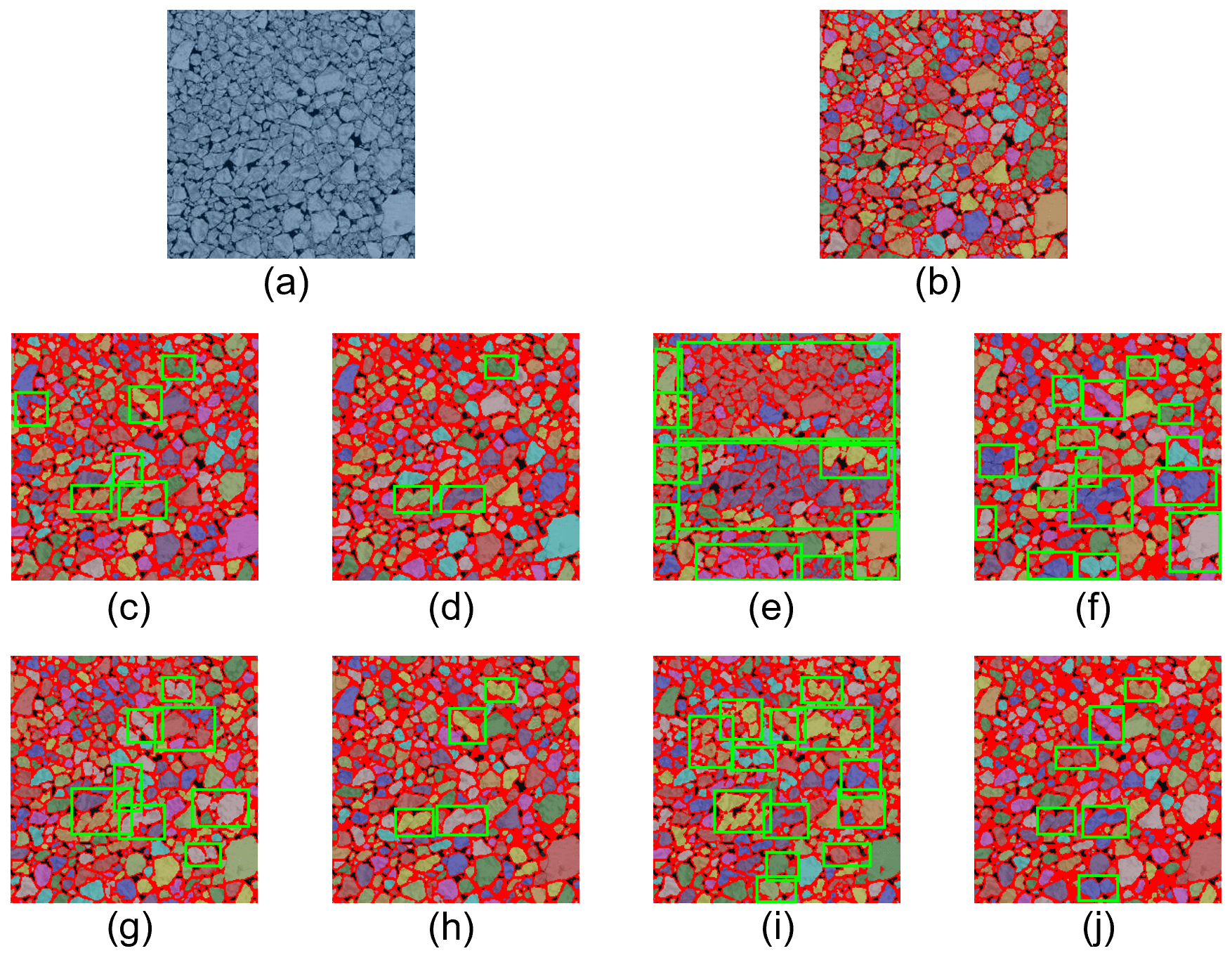
Figure 10Visualization of MIZ image segmentation results by different models. (a) An airborne MIZ image sample. (b) Ground truth, produced by the GVF snake-based method with manual correction. (c) Segmentation by U-Net. (d) Post-processing of (c). (e) Segmentation by ResUNet. (f) Post-processing of (e). (g) Segmentation by U-Net++. (h) Post-processing of (g). (i) Segmentation by ResUNet++. (j) Post-processing of (i). The detected individual ice floes are labelled in different colours, and the detected floe edges are plotted in dark red. Blue rectangle – over-segmentation region; green rectangle – under-segmentation region.
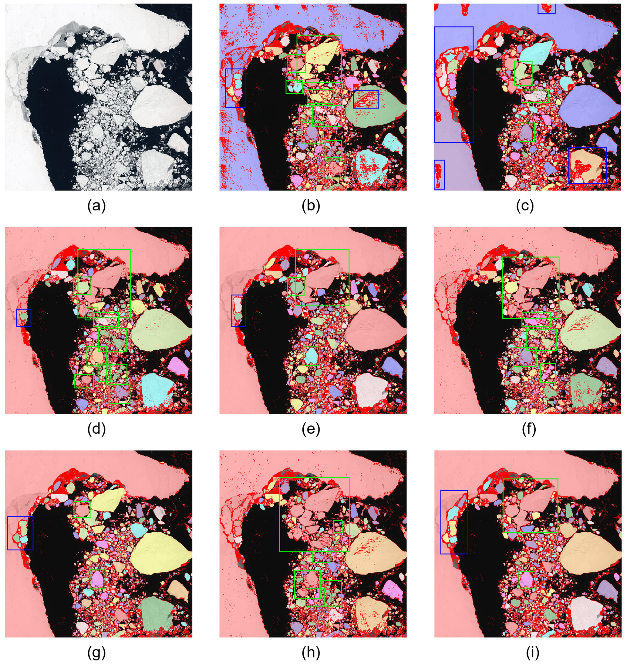
Figure 11Visualization of S2-2 image segmentation results by different models. (a) S2-2 image. (b) Segmentation by U-Net. (c) Post-processing of (b). (d) Segmentation by ResUNet. (e) Post-processing of (d). (f) Segmentation by U-Net++. (g) Post-processing of (f). (h) Segmentation by ResUNet++. (i) Post-processing of (h). The detected individual ice floes are labelled in different colours, and the detected floe edges are plotted in dark red. Blue rectangle – over-segmentation region; green rectangle – under-segmentation region.
5.1.3 Segmentation time
Table 4 lists the average segmentation times of different DL models on our test set. It typically needs more segmentation time as model complexity increases. FCN-8s and FCN-16s took the least segmentation time, while ResUNet, U-Net++, and ResUNet++ needed similar segmentation times that were only 0.4–2 s more than other models. The differences in segmentation time among different DL models were less than an order of magnitude and could be negligible considering the accuracy differences of the models.
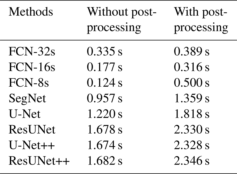
As a compromise, we conclude that the U-Net++ is the most efficient among the other SoA models and is chosen as the DL model for floe instance segmentation.
5.2 1-pixel-wide floe boundary labels versus 2-pixel-wide floe boundary labels
We have widened floe boundaries in labels from 1 to 2 pixels to increase the proportion of the hard-to-train floe boundary class in the training dataset, as seen in Table 5. To prove that boundary widening can improve model performance, we also trained the U-Net++ model on a dataset with 1-pixel-wide ice floe boundary labels and compare it with the model trained on the 2-pixel-wide floe boundary labels. Since the two datasets have different criteria for “ground truth”, the evaluation metrics introduced in Sect. 5.1.1 are not suitable for comparing the performance of the two models. Therefore, we compare the two models only through visual comparison.
Figure 12 shows the segmentation results of S2-2 image by the U-Net++ model trained on 1-pixel-wide floe boundary labels, in which many floe boundary pixels were incorrectly identified as ice floe pixels. Comparing it with Fig. 12a and b, it is easy to see that the model trained on 1-pixel-wide floe boundary labels is more likely to lead to under-segmentation of ice floes, demonstrating that widening the ice floe boundary in labels can effectively improve model performance.
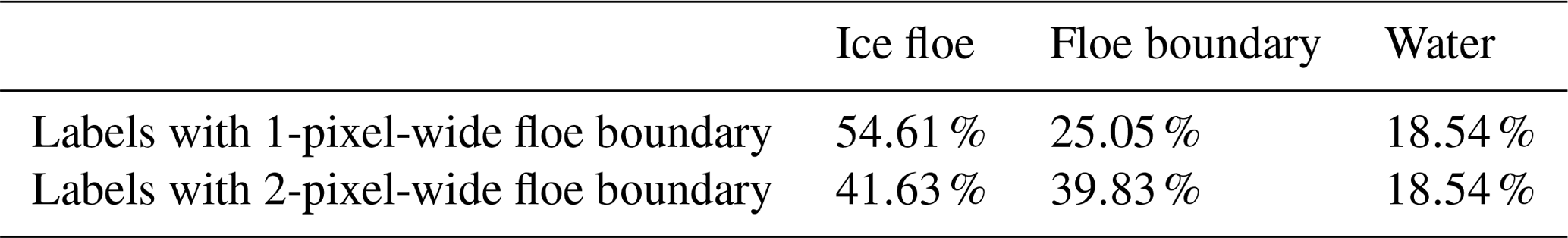
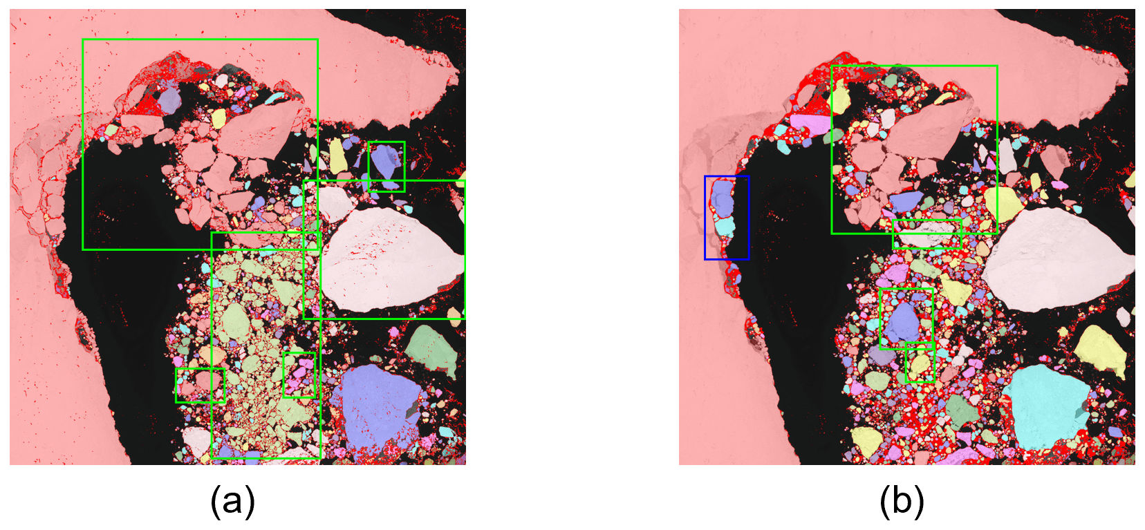
Figure 12S2-2 image segmentation results by U-Net++ model 1-pixel-wide floe boundary labels. (a) Before post-processing. (b) After post-processing. The detected individual ice floes are labelled in different colours, and the detected floe edges are plotted in dark red. Blue rectangle – over-segmentation region; green rectangle – under-segmentation region.
5.3 GVF snake-based method versus U-Net++
5.3.1 Segmentation
Figure 13 shows an example of floe segmentation on a 256 × 256-pixel airborne image with about 177 floes processed by the GVF snake-based method and the U-Net++ model-based approach. In this example, the GVF snake-based method over-segmented 9 ice floes and under-segmented 4 floes, while the U-Net++ model under-segmented 45 floes. The U-Net++ model is less sensitive to the weak edges, and also noise, than the GVF snake-based method, and it is more likely to under-segment ice floes compared with the GVF snake-based method. However, the slight under-segmentation caused by the U-Net++ model can be significantly alleviated by our post-processing method, e.g. leaving only six under-segmented floes as seen in Fig. 13d, while the over-segmentation made by the GVF snake-based method unfortunately cannot be recovered.
Furthermore, due to the nature of the GVF force field, the GVF snake-based method may have difficulty in accurately segmenting both large and small floes when the floes in an image vary greatly in size or shape. Taking Fig. 14b as an example, the GVF snake-based method worked well in segmenting most small ice floes, but it failed in segmenting the largest ice floe in the image, dividing the floe into several pieces. This shortcoming of the GVF snake-based method limits its applications to images other than MIZ images, i.e. the images with floes that are of great diversity in size or shape. As shown in Fig. 15, large floes in the S2-2 image were severely over-segmented with the GVF snake-based method.
Although the U-Net++ model was trained on the pseudo ground truth “annotated” on local-scale MIZ images by the GVF snake-based method, it suffers less from such floe size or shape issues, as seen in Fig. 14c in which both large and small ice floes were well segmented by the U-Net++ model. It can also be extended to process HRO satellite imagery data at global scales as seen in Fig. 11g. The the U-Net++ model-based approach is thus more robust than the GVF snake-based method.
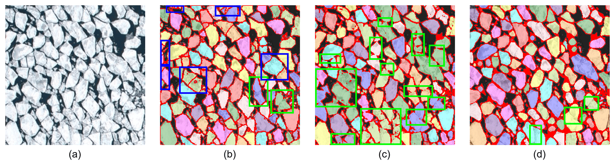
Figure 13Comparison between the GVF snake-based method and U-Net++ on an airborne MIZ image. (a) An airborne MIZ image sample. (b) Segmentation by the GVF snake-based method. (c) Preliminary segmentation by U-net++. (d) Final segmentation after post-processing to (c). Blue rectangle – over-segmentation region; green rectangle – under-segmentation region.
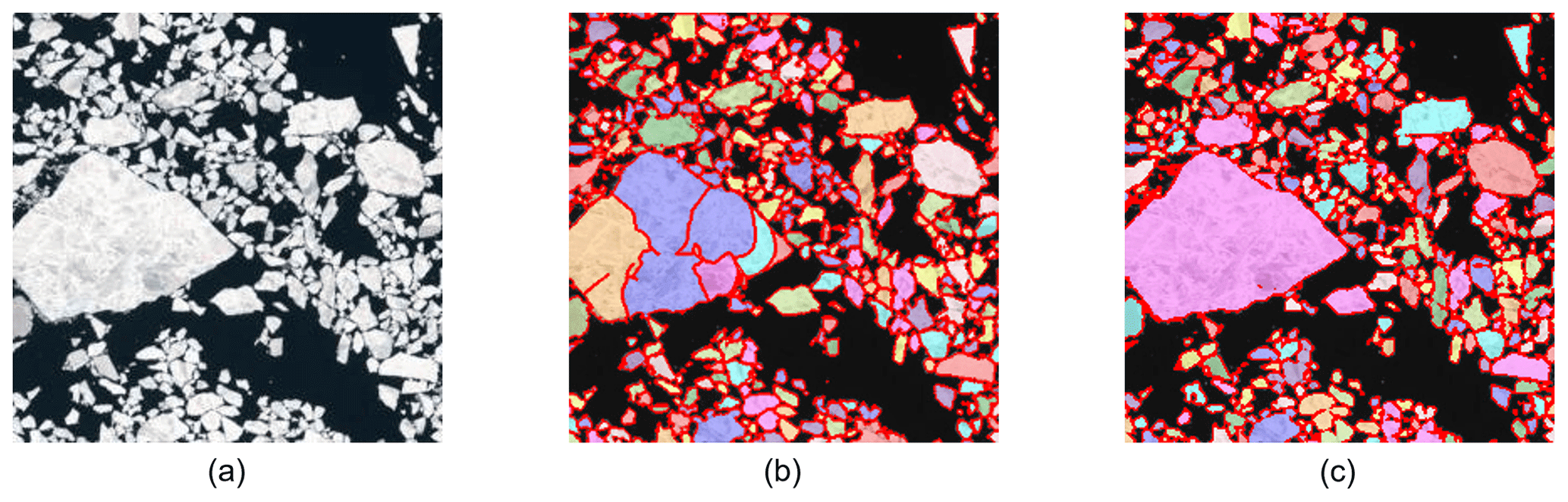
Figure 14Comparison between the GVF snake-based method and U-Net++ on an image containing floes that vary greatly in size and shape. (a) A very small subset of S2-4 image where floes are of various sizes and shapes. (b) Over-segmentation by the GVF snake-based method. (c) Preliminary segmentation by U-Net++. The detected individual ice floes are labelled in different colours, and the detected floe edges are plotted in dark red.
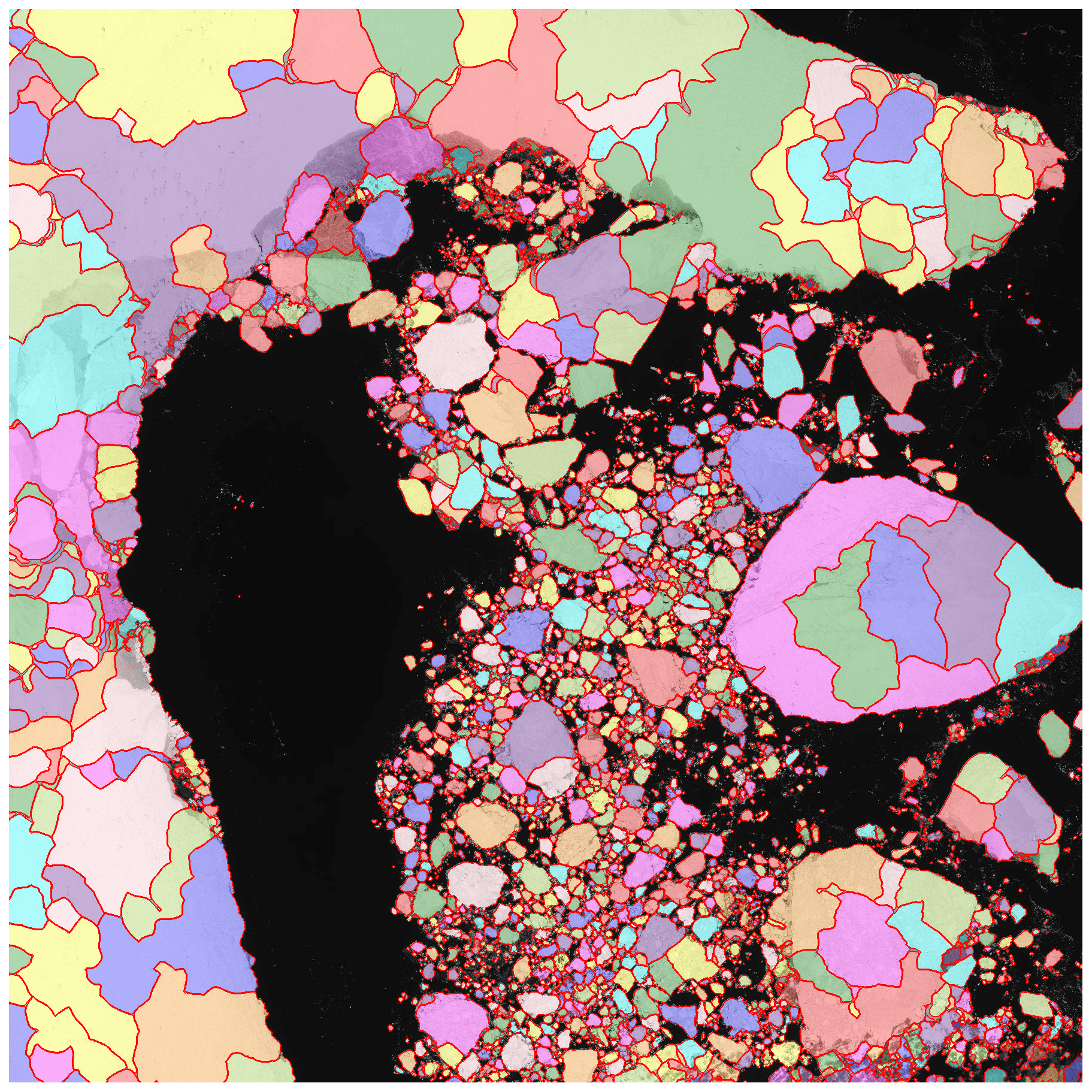
Figure 15Poor segmentation result of S2-2 image produced by the GVF snake-based method. The detected individual ice floes are labelled in different colours, and the detected floe edges are plotted in dark red.
5.3.2 Execution time
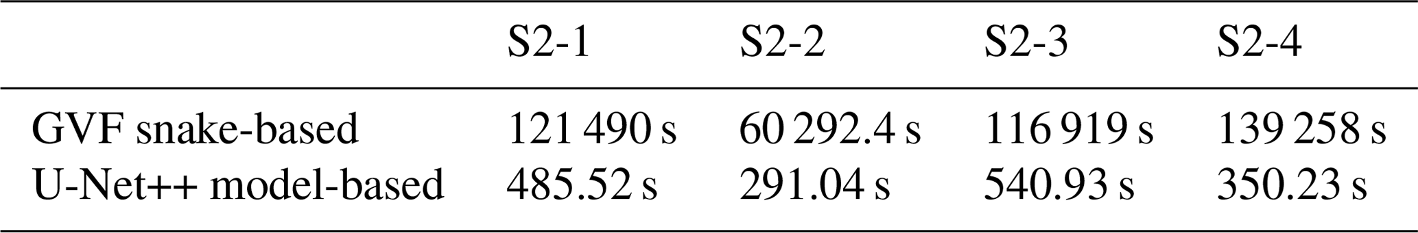
The GVF snake-based is a serial approach that detects ice floes one by one, and it will take a long time to process an image with a large number of ice floes, whereas the U-Net++ model segments individual floes in a parallel manner, meaning that it will use much less execution time. The difference in execution time between the GVF snake-based method and the U-Net++ model-based approach will increase with larger images or the number of floes presented in the image. For example, with the CPU with the configurations illustrated in Sect. 2.2, the GVF snake-based method required around 308.263 s to find all the individual ice floes for Fig. 13a and 60 292.4 s to generate a poor floe segmentation from the S2-2 image. In contrast, the U-Net++ model-based approach took only about 4.234 and 291.050 s to complete the segmentation on these two images with acceptable floe identification results. Table 6 lists the execution times of the GVF snake-based method and the U-Net++ model-based approach on S2 images. It is obvious that the U-Net++ model-based approach is 2–3 orders of magnitude faster than the GVF snake-based method and is more computationally efficient.
Our approach has been applied to the airborne MIZ images and successfully segmented individual ice floes at local scales, even when large numbers of small ice floes are tightly connected, as seen in Fig. 16e–h. Beyond this, our approach was further extended to process HRO satellite imagery data at global scales, where ice floes vary greatly in shape and size. Although the DL model in the approach was trained on the limited dataset consisting only of local-scale MIZ images, it still produced satisfactory floe segmentation results for S2 images, as shown in Fig. 17e–h. With the results of ice floe segmentation, it becomes easier to determine SIC and floe characteristics from the image.
Following the existing studies (Rothrock and Thorndike, 1984; Lu et al., 2008), we use the mean caliper diameter (MCD) as the measure of floe size. The MCD of an ice floe is the average over all angles of the distance between two parallel lines, or calipers, that are set against the floe's side walls. It can be simply calculated by (Toyota et al., 2011)
where Ai is the area of floe i. Many studies have shown that the FSD revealed from aerial or satellite images is basically scale invariant, and the cumulative floe number distribution (CFND), Nc(d), which is the number of floes per unit area with MCD no less than d, can be represented by a power law function:
where Ntotal is the total number of ice floes, and α is the power law exponent used to characterize FSD (Rothrock and Thorndike, 1984; Mellor, 1986; Holt and Martin, 2001; Toyota and Enomoto, 2002; Steer et al., 2008; Lu et al., 2008; Toyota et al., 2011; Perovich and Jones, 2014).
Here, we follow these studies and use power law exponents that fit the CFND curve to characterize FSD. Figures 16i–l and 17i–l show the FSD determination result for local-scale MIZ images and to global-scale S2 images respectively, where α is the slope of the power law curve in logarithmic space. For the FSDs of local-scale MIZ, the curve slope changes greatly with the increase of floe size. α is between 0.6 and 0.7 when the floe size is below 10 m, but it rapidly increases and exceeds 2.4 when floe size is above 10 m. For the FSDs derived from global-scale S2 images, the curve slope increases less with increasing floe size. α averages about 1.4 and 2.0 for floe size smaller and larger than 1000 m, respectively.
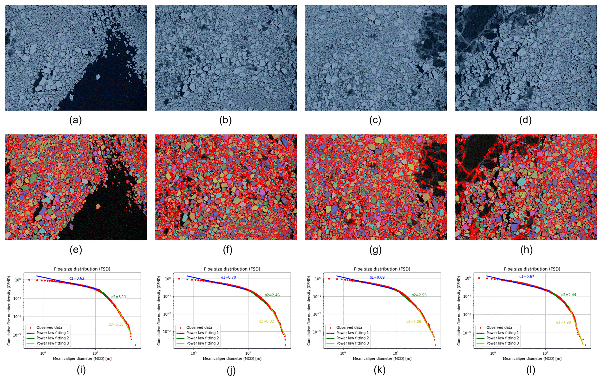
Figure 16Determining and characterizing FSD from local-scale airborne MIZ images. (a) MIZ-1 image; (b) MIZ-2 image; (c) MIZ-3 image; (d) MIZ-4 image; (e) floe segmentation of MIZ-1 image, SIC=63.6546 %; (f) floe segmentation of MIZ-2 image, SIC=85.5286 %; (g) floe segmentation of MIZ-3 image, SIC=84.1209 %; (h) floe segmentation of MIZ-4 image, SIC=73.7770 %; (i) FSD of MIZ-1 image; (j) FSD of MIZ-2 image; (k) FSD of MIZ-3 image; and (l) FSD of MIZ-4 image. The detected individual ice floes are labelled in different colours, and the detected floe edges are plotted in dark red.
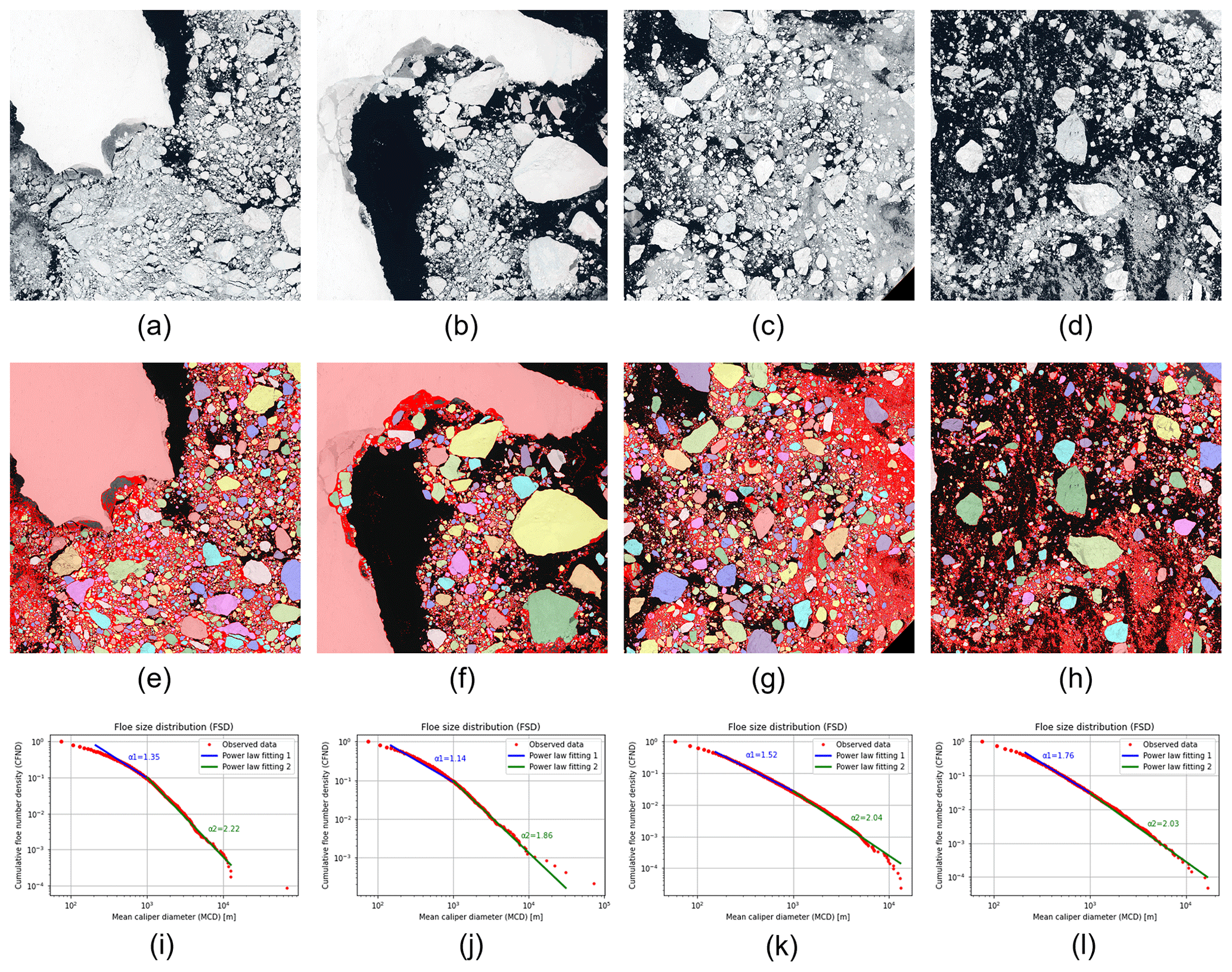
Figure 17Determining and characterizing FSD from global-scale S2 images. (a) S2-1 image; (b) S2-2 image; (c) S2-3 image; (d) S2-4 image; (e) floe segmentation of S2-1 image, SIC=86.6861 %; (f) floe segmentation of S2-2 image, SIC=65.7758 %; (g) floe segmentation of S2-3 image, SIC=76.9105 %; (h) floe segmentation of S2-4 image, SIC=51.5449 %; (i) FSD of S2-1 image; (j) FSD of S2-2 image; (k) FSD of S2-3 image; and (l) FSD of S2-4 image.The detected individual ice floes are labelled in different colours, and the detected floe edges are plotted in dark red.
In applying our approach to both local-scale airborne MIZ images and to global-scale HRO satellite image data, we can see that there are inherent limits to the resulting FSD. The MIZ images are on average 0.22 m resolution, with a footprint 1.225×0.689 km2. Using the floe size terminology of the operational monitoring of the World Meteorological Organization (JCOMM Expert Team on Sea Ice, 2014), this makes them ideal for determining the distribution of pancake ice, small ice cake, brash ice, and agglomerated brash, and sizes up to small floes of width 100 m. However once floes exceed this size, i.e. medium-sized floes, it is likely that there will be a cut-off in the FSD as floes become cropped by the image boundaries.
In contrast, the S2 images are 10 m resolution with a footprint of 110.0×110.0 km2. These cover the upper part of the FSD, from small floes down to 20 m width through to vast floes where the width is up to 10 km. Only the smallest floes size categories, from pancake ice through to ice cakes, are not resolved. This broader range of foe sizes are preferable for navigational applications and for comparison and validation of lower-resolution sea ice datasets, particularly SIC from passive microwave sensors and ice charts. The spatial scales are also relevant for integration with sea ice freeboard measurement from NASA ICESat-2 (Kwok et al., 2023), allowing ice floe mass to be assessed in areas where there are coincident data.
We have achieved automatic labelling of dataset for training a DL semantic segmentation model for ice floe instance segmentation, where classical image processing techniques were utilized to replace human labelling of individual ice floes and automatically generate “ground truth” from the airborne MIZ images at local scales. A post-processing algorithm is also proposed to refine the model outputs. Our approach has been applied to both airborne and satellite sea ice floe images to determine FSDs from local to global scales and from low to high SIC. Our approach can be used to analyse optical sea ice images for determining FSDs and other floe characteristics for use in climate, meteorology, environment, etc. Especially for marine operations, our approach provides the possibility of online monitoring of in situ ice conditions and early warning of risky ice floes, thus offering better data for path planning and improving maritime safety.
In the application of spatial and temporal extraction of ice floe from S2 images, our approach yields superior floe instance segmentation results for the floes with relatively flat surfaces and is proven to be time-efficient and effective. However, when the floes contain many melt ponds (e.g. summer floes), our approach tends to over-segment them. This is because the DL model was trained on MIZ images containing only three classes: ice floe, ice floe boundary, and water. The model therefore has no experience in handling melt ponds. Since the pixel intensities of melt ponds are between those of ice floe and water (Lu et al., 2018), the DL model often misidentifies melting ponds as floe boundaries, which easily leads to over-segmentation. An idea to reduce the misidentification of melt ponds is to potentially use additional sea ice classification methods to detect melt pond regions (Miao et al., 2015; Sudakow et al., 2022), then catalogue these melt pond pixels to the class of floe in DL prediction, and finally refine the floe segmentation using the proposed post-processing.
Since the current DL model also does not consider the class of cloud and cloud shade, our approach has limitations in processing the floe images with clouds, where the cloud and cloud shade may be mistaken as ice floe and boundaries respectively. Existing cloud masking methods, Sen2Cor (Muller-Wilm, 2012) and Fmask (Zhu et al., 2015), can help classify clouds in Sentinel-2 images. Then the ice floes detected near the cloud regions which are likely to be incorrectly segmented can be excluded when determining FSDs.
Post-processing is used to refine the floe segmentation, such as removing “holes” in large floes, preserving floe shape and separating potentially under-segmented floes that may affect FSDs. This is a necessary step to maintain the integrity of the ice floe, especially when the surface of the floe is noisy, i.e. contains by small melt ponds, partially covered by small clouds, etc. In our post-processing, we have proposed criteria to automatically check whether the detected floes are well segmented to decide whether to perform subsequent morphological opening and closing. The area cut-off threshold Ta for finding the potential under-segmented floes and the area threshold for finding floes require a smooth shape, which are two main parameters in our post-processing that need to be adjusted according to image scale and/or practical application needs, while the solidity cut-off threshold Ts kept constant at 0.85. The pure morphological operations adopted in our post-processing often require extensive manual parameter tuning to segment floes even from a single image, since they operate on the binarized image and rely on how well the edges are detected between connected floes. As the DL method detects more accurate floe boundaries, morphological operations in our post-processing become less dependent on parameters in refining floe segmentation (a disc-shaped structuring element with a radius of 4 pixels was used in the morphological operations), making the entire process more automated.
So far, we have not found a good solution to the problem of ambiguous over-segmentation in a single optical floe image (e.g. the middle-left part of the biggest floe in S2-2 image in Fig. 11). A series of images of the same area over different periods or other types of the remote sensing data may be needed to help determine whether the floe is over-segmented.
DL techniques require a large annotated dataset to obtain a powerful DL models. Unlike other popular image processing tasks that already have large numbers of public datasets (Lin et al., 2014; Deng et al., 2009; Kuznetsova et al., 2020; Kaggle Datasets, 2023), obtaining large labelled image datasets for the ice floe segmentation task is very challenging. This limits the development of deep learning technique in ice floe segmentation, and it is therefore desired to establish a dataset for floe segmentation application. Due to the limited training dataset, the current DL model in our approach has some limitations. However, it still can be utilized as a “higher version” of “annotation tool” and produce more “ground truth” from a wide variety of ice image data sources, contributing to the establishment of datasets suitable for ice floe segmentation tasks, as well as further training more robust DL models for obtaining more accurate ice parameters from images.
Our floe mapping approach can be applied to widely available and free to access, near-real-time (NRT) HRO images from Copernicus Sentinel-2. Previous studies, for example, have been limited to airborne or declassified military satellite images (e.g. MEDEA used in Denton and Timmermans, 2022 and Wang et al., 2023) or X-band SAR (Ren et al., 2015; Hwang et al., 2017). Neither of these can provide the regional, NRT coverage to make them viable in operational monitoring for maritime safety. We appreciate that HRO is still cloud and nighttime darkness limited, but the benefit of using Sentinel-2 is in combination with other approaches, especially SAR-based classifications, when cloud-free periods allow. We look forward to the darkness limitation being solved with the future Copernicus Land Surface Temperature Monitoring (LSTM) mission.
Examples of NetCDF files of S2 images segmented for ice floes and containing both georeferenced gridded and vector polygon data can be downloaded from https://thredds.met.no/thredds/catalog/digitalseaice/catalog.html (Hughes, 2023a). These contain ancillary data including a panchromatic quick look of the original S2 image, Sen2Cor (Muller-Wilm, 2012) and Fmask (Zhu et al., 2015) cloud masks, and a table of floe metrics including area, perimeter and long-axis lengths, and orientation.
A catalogue GeoJSON file of the NetCDF files, to aid geospatial and temporal locating of the examples, can be found at https://bit.ly/s2floemaps (Hughes, 2023b). Further examples will be added, with the intention of making this a routine, operationally available product in the future.
QZ: conceptualization, methodology, implementation, writing – original draft. NH: project leader, quality control, writing – review and editing.
The contact author has declared that neither of the authors has any competing interests.
Publisher's note: Copernicus Publications remains neutral with regard to jurisdictional claims made in the text, published maps, institutional affiliations, or any other geographical representation in this paper. While Copernicus Publications makes every effort to include appropriate place names, the final responsibility lies with the authors.
This research work was supported by funding from the European Union's Horizon 2020 research and innovation programme under grant agreement 825258, the From Copernicus Big Data to Extreme Earth Analytics (ExtremeEarth, https://earthanalytics.eu/, last access: 20 December 2023) project. Further work to refine the processing, and develop the NetCDF outputs, was conducted under the Norwegian Research Council project 328960 Multi-scale integration and digitalization of Arctic sea ice observations and prediction models (DigitalSeaIce, https://www.ntnu.edu/digitalseaice, last access: 20 December 2023) project. We would also like to thank the Centre for Research-based Innovation (CRI-SFI) Sustainable Arctic Marine and Coastal Technology (SAMCoT) research centre funded by the Research Council of Norway (RCN project number 203471) for providing aerial MIZ image data to our work.
This research has been supported by the HORIZON EUROPE European Innovation Council (grant no. 825258) and Norwegian Research Council (grant no. 328960).
This paper was edited by Bin Cheng and reviewed by three anonymous referees.
Copernicus Open Access Hub: https://scihub.copernicus.eu, last access: 20 December 2023. a
Kaggle Datasets: https://www.kaggle.com/datasets, last access: 20 December 2023. a
Badrinarayanan, V., Kendall, A., and Cipolla, R.: SegNet: A Deep Convolutional Encoder-Decoder Architecture for Image Segmentation, IEEE T. Pattern Anal., 39, 2481–2495, https://doi.org/10.1109/TPAMI.2016.2644615, 2017. a, b, c
Banfield, J.: Automated tracking of ice floes: A stochastic approach, IEEE T. Geosci. Remote, 29, 905–911, https://doi.org/10.1109/36.101369, 1991. a
Banfield, J. D. and Raftery, A. E.: Ice floe identification in satellite images using mathematical morphology and clustering about principal curves, J. Am. Stat. Assoc., 87, 7–16, https://doi.org/10.2307/2290446, 1992. a
Blunt, J., Garas, V., Matskevitch, D., Hamilton, J., and Kumaran, K.: Image Analysis Techniques for High Arctic, Deepwater Operation Support, in: OTC Arctic Technology Conference, Houston, Texas, USA, https://doi.org/10.4043/23825-MS, 2012. a
Bolya, D., Zhou, C., Xiao, F., and Lee, Y. J.: YOLACT: Real-Time Instance Segmentation, in: IEEE International Conference on Computer Vision (ICCV), Seoul, Korea (South), IEEE, 9156–9165, https://doi.org/10.1109/ICCV.2019.00925, 2019. a, b
Cai, J., Ding, S., Zhang, Q., Liu, R., Zeng, D., and Zhou, L.: Broken ice circumferential crack estimation via image techniques, Ocean Eng., Ocean Eng., 259, 111735, https://doi.org/10.1016/j.oceaneng.2022.111735, 2022. a, b
Chai, Y., Ren, J., Hwang, B., Wang, J., Fan, D., Yan, Y., and Zhu, S.: Texture-sensitive superpixeling and adaptive thresholding for effective segmentation of sea ice floes in high-resolution optical images, IEEE J. Sel. Top. Appl., 14, 577–586, https://doi.org/10.1109/JSTARS.2020.3040614, 2020. a
Deng, J., Dong, W., Socher, R., Li, L.-J., Li, K., and Fei-Fei, L.: Imagenet: A large-scale hierarchical image database, in: 2009 IEEE Conference on Computer Vision and Pattern Recognition (CVPR), IEEE, 248–255, https://doi.org/10.1109/CVPR.2009.5206848, 2009. a
Denton, A. A. and Timmermans, M.-L.: Characterizing the sea-ice floe size distribution in the Canada Basin from high-resolution optical satellite imagery, The Cryosphere, 16, 1563–1578, https://doi.org/10.5194/tc-16-1563-2022, 2022. a, b
Drusch, M., Del Bello, U., Carlier, S., Colin, O., Fernandez, V., Gascon, F., Hoersch, B., Isola, C., Laberinti, P., Martimort, P., Meygret, A., Spoto, F., Sy, O., Marchese, F., and Bargellini, P.: Sentinel-2: ESA's optical high-resolution mission for GMES operational services, Remote Sens. Environ., 120, 25–36, https://doi.org/10.1016/j.rse.2011.11.026, 2012. a
Gonçalves, B. C. and Lynch, H. J.: Fine-Scale Sea Ice Segmentation for High-Resolution Satellite Imagery with Weakly-Supervised CNNs, Remote Sens., 13, 3562, https://doi.org/10.3390/rs13183562, 2021. a
Goutte, C. and Gaussier, E.: A probabilistic interpretation of precision, recall and F-score, with implication for evaluation, in: European conference on information retrieval, Springer, 345–359, https://doi.org/10.1007/978-3-540-31865-1_25, 2005. a
He, K., Gkioxari, G., Dollár, P., and Girshick, R.: Mask R-CNN, in: IEEE International Conference on Computer Vision (ICCV), Venice, Italy, IEEE, 2980–2988, https://doi.org/10.1109/ICCV.2017.322, 2017. a, b
Holt, B. and Martin, S.: The effect of a storm on the 1992 summer sea ice cover of the Beaufort, Chukchi, and East Siberian Seas, J. Geophys. Res.-Oceans, 106, 1017–1032, https://doi.org/10.1029/1999JC000110, 2001. a
Horvat, C. and Tziperman, E.: Understanding Melting due to Ocean Eddy Heat Fluxes at the Edge of Sea-Ice Floes, Geophys. Res. Lett., 45, 9721–9730, https://doi.org/10.1029/2018GL079363, 2018. a
Huang, G., Liu, Z., Van Der Maaten, L., and Weinberger, K. Q.: Densely Connected Convolutional Networks, in: 2017 IEEE Conference on Computer Vision and Pattern Recognition (CVPR), Honolulu, HI, USA, IEEE, 2261–2269, https://doi.org/10.1109/CVPR.2017.243, 2017. a
Hughes, N.: NetCDF files of Sentinel-2 floe image segmentation, https://thredds.met.no/thredds/catalog/digitalseaice/catalog.html, last access: 20 December 2023a. a
Hughes, N.: A catalogue GeoJSON file of the NetCDF files, https://drive.google.com/file/d/1xV8_Xomin8tuTizf0pXnZvF8hwIUY9lt/view, last access: 20 December 2023b. a
Hwang, B., Ren, J., McCormack, S., Berry, C., Ayed, I. B., Graber, H. C., and Aptoula, E.: A practical algorithm for the retrieval of floe size distribution of Arctic sea ice from high-resolution satellite Synthetic Aperture Radar imagery, Elem. Sci. Anth., 5, 38, https://doi.org/10.1525/elementa.154, 2017. a
JCOMM Expert Team on Sea Ice: Sea-Ice Nomenclature: snapshot of the WMO Sea Ice Nomenclature WMO No. 259, volume 1 – Terminology and Codes; Volume II – Illustrated Glossary and III – International System of Sea-Ice Symbols), Tech. rep., WMO-JCOMM, https://doi.org/10.25607/OBP-1515, 2014. a
Jeppesen, J. H., Jacobsen, R. H., Inceoglu, F., and Toftegaard, T. S.: A cloud detection algorithm for satellite imagery based on deep learning, Remote Sens. Environ., 229, 247–259, https://doi.org/10.1016/j.rse.2019.03.039, 2019. a
Jha, D., Smedsrud, P. H., Riegler, M. A., Johansen, D., De Lange, T., Halvorsen, P., and Johansen, H. D.: Resunet++: An advanced architecture for medical image segmentation, in: 2019 IEEE International Symposium on Multimedia (ISM), San Diego, CA, USA, IEEE, 225–2255, https://doi.org/10.1109/ISM46123.2019.00049, 2019. a
Jing, L. and Tian, Y.: Self-supervised visual feature learning with deep neural networks: A survey, IEEE T. Pattern Anal., 43, 4037–4058, https://doi.org/10.1109/TPAMI.2020.2992393, 2021. a, b
Kamrul Hasan, S. M. and Linte, C. A.: U-NetPlus: A Modified Encoder-Decoder U-Net Architecture for Semantic and Instance Segmentation of Surgical Instruments from Laparoscopic Images, in: 2019 41st Annual International Conference of the IEEE Engineering in Medicine and Biology Society (EMBC), Berlin, Germany, IEEE, 7205–7211, https://doi.org/10.1109/EMBC.2019.8856791, 2019. a, b
Khaleghian, S., Ullah, H., Kræmer, T., Hughes, N., Eltoft, T., and Marinoni, A.: Sea Ice Classification of SAR Imagery Based on Convolution Neural Networks, Remote Sens., 13, 1734, https://doi.org/10.3390/rs13091734, 2021. a
Kisantal, M., Wojna, Z., Murawski, J., Naruniec, J., and Cho, K.: Augmentation for small object detection, arXiv [preprint], https://doi.org/10.48550/arXiv.1902.07296, 2019. a
Kuznetsova, A., Rom, H., Alldrin, N., Uijlings, J., Krasin, I., Pont-Tuset, J., Kamali, S., Popov, S., Malloci, M., Kolesnikov, A., Tom Duerig, T., and Ferrari, V.: The open images dataset v4: Unified image classification, object detection, and visual relationship detection at scale, Int. J. Comput. Vis., 128, 1956–1981, 2020. a
Kwok, R., Petty, A. A., Cunningham, G., Markus, T., Hancock, D., Ivanoff, A., Wimert, J., Bagnardi, M., Kurtz, N., and the ICESat-2 Science Team: ATLAS/ICESat-2 L3A Sea Ice Freeboard, Version 6, National Snow and Ice Data Center (NSIDC) [data set], https://doi.org/10.5067/ATLAS/ATL10.006, 2023. a
Lin, T., Maire, M., Belongie, S. J., Bourdev, L. D., Girshick, R. B., Hays, J., Perona, P., Ramanan, D., Dollár, P., and Zitnick, C. L.: Microsoft COCO: Common Objects in Context, CoRR, arXiv [preprint], https://doi.org/10.48550/arXiv.1405.0312, 2014. a
Long, J., Shelhamer, E., and Darrell, T.: Fully Convolutional Networks for Semantic Segmentation, in: Proceedings of the IEEE Conference on Computer Vision and Pattern Recognition (CVPR), Boston, MA, USA, 3431–3440, https://doi.org/10.1109/CVPR.2015.7298965, 2015. a, b, c, d, e
Lu, P., Li, Z., Zhang, Z., and Dong, X.: Aerial observations of floe size distribution in the marginal ice zone of summer Prydz Bay, J. Geophys. Res.-Oceans, 113, C02011, https://doi.org/10.1029/2006JC003965, 2008. a, b
Lu, P., Leppäranta, M., Cheng, B., Li, Z., Istomina, L., and Heygster, G.: The color of melt ponds on Arctic sea ice, The Cryosphere, 12, 1331–1345, https://doi.org/10.5194/tc-12-1331-2018, 2018. a
Lubbad, R., Løset, S., Lu, W., Tsarau, A., and van den Berg, M.: An overview of the Oden Arctic Technology Research Cruise 2015 OATRC2015 and numerical simulations performed with SAMS driven by data collected during the cruise, Cold Reg. Sci. Technol., 156, 1–22, https://doi.org/10.1016/j.coldregions.2018.04.006, 2018. a, b
Manucharyan, G. E. and Thompson, A. F.: Submesoscale sea ice-ocean interactions in marginal ice zones, J. Geophys. Res.-Oceans, 122, 9455–9475, https://doi.org/10.1002/2017JC012895, 2017. a
Marchenko, N.: Russian Arctic Seas: Navigational conditions and accidents, Springer Berlin Heidelberg, ISBN 9783642221255, https://doi.org/10.1007/978-3-642-22125-5, 2012. a
Mellor, M.: Mechanical behavior of sea ice, in: The geophysics of sea ice, Springer, 165–281, https://doi.org/10.1007/978-1-4899-5352-0_3, 1986. a
Miao, X., Xie, H., Ackley, S. F., Perovich, D. K., and Ke, C.: Object-based detection of Arctic sea ice and melt ponds using high spatial resolution aerial photographs, Cold Reg. Sci. Technol., 119, 211–222, 2015. a
Mironov, Y.: Ice Phenomena Threatening Arctic Shipping, Backbone Publishing Co., ISBN 0984786422, https://www.backbonepublishing.com/home/arctic-antarctic/ice-phenomena-threatening-arctic-shipping (last access: 20 December 2023), 2012. a
Muller-Wilm, U.: Sentinel-2 MSI – Level 2A Products Algorithm Theoretical Basis Document, ESA Report 2012, Tech. rep., ref S2PAD-ATBD-0001 Issue 2.0, 2012. a, b
Nagi, A. S., Kumar, D., Sola, D., and Scott, K. A.: RUF: Effective Sea Ice Floe Segmentation Using End-to-End RES-UNET-CRF with Dual Loss, Remote Sens., 13, 2460, https://doi.org/10.3390/rs13132460, 2021. a
Nose, T., Waseda, T., Kodaira, T., and Inoue, J.: Satellite-retrieved sea ice concentration uncertainty and its effect on modelling wave evolution in marginal ice zones, The Cryosphere, 14, 2029–2052, https://doi.org/10.5194/tc-14-2029-2020, 2020. a
Notz, D. and SIMIP Community: Arctic sea ice in CMIP6, Geophys. Res. Lett., 47, e2019GL086749, https://doi.org/10.1029/2019GL086749, 2020. a
Perovich, D. K. and Jones, K. F.: The seasonal evolution of sea ice floe size distribution, J. Geophys. Res.-Oceans, 119, 8767–8777, https://doi.org/10.1002/2014JC010136, 2014. a
Ren, J., Hwang, B., Murray, P., Sakhalkar, S., and McCormack, S.: Effective SAR sea ice image segmentation and touch floe separation using a combined multi-stage approach, in: 2015 IEEE International Geoscience and Remote Sensing Symposium (IGARSS), IEEE, 1040–1043, https://doi.org/10.1109/IGARSS.2015.7325947, 2015. a
Ronneberger, O., Fischer, P., and Brox, T.: U-Net: Convolutional Networks for Biomedical Image Segmentation, in: Medical Image Computing and Computer-Assisted Intervention (MICCAI), Springer, 234–241, https://doi.org/10.1007/978-3-319-24574-4_28, 2015. a, b, c
Rothrock, D. and Thorndike, A.: Measuring the sea ice floe size distribution, J. Geophys. Res.-Oceans, 89, 6477–6486, https://doi.org/10.1029/JC089iC04p06477, 1984. a, b, c
Soh, L.-K., Tsatsoulis, C., and Holt, B.: Identifying Ice Floes and Computing Ice Floe Distributions in SAR Images, in: Analysis of SAR Data of the Polar Oceans, edited by: Tsatsoulis, C. and Kwok, R., Springer, Berlin, 9–34, https://doi.org/10.1007/978-3-642-60282-5_2, 1998. a
Squire, V. A., Dugan, J. P., Wadhams, P., Rottier, P. J., and Liu, A. K.: Of ocean waves and sea ice, Annu. Rev. Fluid Mech., 27, 115–168, https://doi.org/10.1146/annurev.fl.27.010195.000555, 1995. a
Steer, A., Worby, A., and Heil, P.: Observed changes in sea-ice floe size distribution during early summer in the western Weddell Sea, Deep-Sea Res. Pt. II, 55, 933–942, https://doi.org/10.1016/j.dsr2.2007.12.016, 2008. a, b
Sudakow, I., Asari, V. K., Liu, R., and Demchev, D.: MeltPondNet: A Swin Transformer U-Net for Detection of Melt Ponds on Arctic Sea Ice, IEEE J. Sel. Top. Appl., 15, 8776–8784, 2022. a
Toyota, T. and Enomoto, H.: Analysis of sea ice floes in the Sea of Okhotsk using ADEOS/AVNIR images, in: Proceedings of the 16th IAHR International Symposium on Ice, Dunedin, New Zealand, 211–217, 2002. a
Toyota, T., Takatsuji, S., and Nakayama, M.: Characteristics of sea ice floe size distribution in the seasonal ice zone, Geophys. Res. Lett., 33, L02616, https://doi.org/10.1029/2005GL024556, 2006. a, b
Toyota, T., Haas, C., and Tamura, T.: Size distribution and shape properties of relatively small sea-ice floes in the Antarctic marginal ice zone in late winter, Deep-Sea Res. Pt. II, 58, 1182–1193, https://doi.org/10.1016/j.dsr2.2010.10.034, 2011. a, b, c
Toyota, T., Kohout, A., and Fraser, A. D.: Formation processes of sea ice floe size distribution in the interior pack and its relationship to the marginal ice zone off East Antarctica, Deep-Sea Res. Pt. II, 131, 28–40, https://doi.org/10.1016/j.dsr2.2015.10.003, 2016. a
Wang, Y., Holt, B., Erick Rogers, W., Thomson, J., and Shen, H. H.: Wind and wave influences on sea ice floe size and leads in the Beaufort and Chukchi Seas during the summer-fall transition 2014, J. Geophys. Res.-Oceans, 121, 1502–1525, https://doi.org/10.1002/2015JC011349, 2016. a
Wang, Y., Hwang, B., Bateson, A. W., Aksenov, Y., and Horvat, C.: Summer sea ice floe perimeter density in the Arctic: high-resolution optical satellite imagery and model evaluation, The Cryosphere, 17, 3575–3591, https://doi.org/10.5194/tc-17-3575-2023, 2023. a
Zhang, Q.: Sea Ice Image Processing with MATLAB, Norwegian University of Science and Technology (NTNU) [code], https://www.ntnu.edu/imt/books/sea_ice_image_processing_with_matlab (last access: 20 December 2023), 2018. a
Zhang, Q.: Image Processing for Sea Ice Parameter Identification from Visual Images, in: Handbook of Pattern Recognition and Computer Vision, edited by: Chen, C. H., World Scientific, 231–250, https://doi.org/10.1142/9789811211072_0012, 2020. a, b
Zhang, Q. and Skjetne, R.: Image Processing for Identification of Sea-Ice Floes and the Floe Size Distributions, IEEE T. Geosci. Remote, 53, 2913–2924, https://doi.org/10.1109/TGRS.2014.2366640, 2015. a
Zhang, Q. and Skjetne, R.: Sea Ice Image Processing with MATLAB®, CRC Press, Taylor & Francis, USA, ISBN 978-1-1380-3266-8, 2018. a, b, c
Zhang, Q., Skjetne, R., Løset, S., and Marchenko, A.: Digital Image Processing for Sea Ice Observation in Support to Arctic DP Operation, in: Proceedings of 31st International Conference on Ocean, Offshore and Arctic Engineering, ASME, Rio de Janeiro, Brazil, https://doi.org/10.1115/OMAE2012-83860, 2012. a
Zhang, Q., Skjetne, R., and Su, B.: Automatic Image Segmentation for Boundary Detection of Apparently Connected Sea-ice Floes, in: Proceedings of the 22nd International Conference on Port and Ocean Engineering under Arctic Conditions, Espoo, Finland, https://doi.org/10.4173/mic.2014.4.6, 2013. a
Zhang, T., Yang, Y., Shokr, M., Mi, C., Li, X.-M., Cheng, X., and Hui, F.: Deep Learning Based Sea Ice Classification with Gaofen-3 Fully Polarimetric SAR Data, Remote Sens., 13, 1452, https://doi.org/10.3390/rs13081452, 2021. a
Zhang, Z., Liu, Q., and Wang, Y.: Road Extraction by Deep Residual U-Net, IEEE Geosci. Remote Sens. Lett., 15, 749–753, https://doi.org/10.1109/LGRS.2018.2802944, 2018. a, b
Zhou, Z., Rahman Siddiquee, M. M., Tajbakhsh, N., and Liang, J.: UNet++: A Nested U-Net Architecture for Medical Image Segmentation, in: Deep Learning in Medical Image Analysis and Multimodal Learning for Clinical Decision Support, Springer, 3–11, https://doi.org/10.1007/978-3-030-00889-5_1, 2018. a, b, c
Zhou, Z., Siddiquee, M. M. R., Tajbakhsh, N., and Liang, J.: UNet++: Redesigning Skip Connections to Exploit Multiscale Features in Image Segmentation, IEEE T. Medical Imaging, 39, 1856–1867, https://doi.org/10.1109/TMI.2019.2959609, 2020. a
Zhou, Z.-H.: A brief introduction to weakly supervised learning, Natl. Sci. Rev., 5, 44–53, https://doi.org/10.1093/nsr/nwx106, 2017. a, b
Zhu, Z., Wang, S., and Woodcock, C. E.: Improvement and expansion of the Fmask algorithm: cloud, cloud shadow, and snow detection for Landsats 4–7, 8, and Sentinel 2 images, Remote Sens. Environ., 159, 269–277, https://doi.org/10.1016/j.rse.2014.12.014, 2015. a, b
These severe misannotations by the GVF snake-based method occurred in non-MIZ regions and regions blurred by water vapour in the images. This can be avoided if all the training images are clear and have no non-MIZ regions.
- Abstract
- Introduction
- Datasets and computational resources
- Methodology
- Implementation details
- Method comparisons
- Ice floe segmentation results and floe size distributions
- Discussion and conclusion
- Data availability
- Author contributions
- Competing interests
- Disclaimer
- Acknowledgements
- Financial support
- Review statement
- References