Four North American glaciers advanced past their modern positions thousands of years apart in the Holocene

There is unambiguous evidence that glaciers have retreated from their 19th century positions, but it is less clear how far glaciers have retreated relative to their long-term Holocene fluctuations. Glaciers in western North America are thought to have advanced from minimum positions in the Early Holocene to maximum positions in the Late Holocene. We assess when four North American glaciers, located between 38–60^∘ N, were larger or smaller than their modern (2018–2020 CE) positions during the Holocene. We measured 26 paired cosmogenic in situ ¹⁴C and ¹⁰Be concentrations in recently exposed proglacial bedrock and applied a Monte Carlo forward model to reconstruct plausible bedrock exposure–burial histories. We find that these glaciers advanced past their modern positions thousands of years apart in the Holocene: a glacier in the Juneau Icefield (BC, Canada) at ∼2 ka, Kokanee Glacier (BC, Canada) at ∼6 ka, and Mammoth Glacier (WY, USA) at ∼1 ka; the fourth glacier, Conness Glacier (CA, USA), was likely larger than its modern position for the duration of the Holocene until present. The disparate Holocene exposure–burial histories are at odds with expectations of similar glacier histories given the presumed shared climate forcings of decreasing Northern Hemisphere summer insolation through the Holocene followed by global greenhouse gas forcing in the industrial era. We hypothesize that the range in histories is the result of unequal amounts of modern retreat relative to each glacier's Holocene maximum position, rather than asynchronous Holocene advance histories. We explore the influence of glacier hypsometry and response time on glacier retreat in the industrial era as a potential cause of the non-uniform burial durations. We also report mean abrasion rates at three of the four glaciers: Juneau Icefield Glacier (0.3±0.3 mm yr⁻¹), Kokanee Glacier (0.04±0.03 mm yr⁻¹), and Mammoth Glacier (0.2±0.2 mm yr⁻¹).

1 Introduction

As global temperatures have increased since the industrial era, alpine glaciers have receded worldwide to lengths not observed since record-keeping began in the 17th century (Oerlemans, 2005). Declining glacial meltwater poses threats to agriculture, human consumption, and biodiversity (Milner et al., 2017; Huss et al., 2017) with severe consequences for people who live in high mountain regions (Masson-Delmotte et al., 2021). Although significant strides have been made towards projecting glacier disappearance (e.g., Rounce et al., 2023), there is ample room to reduce uncertainty in these projections by studying past glacier length fluctuations in response to climate change. Notably, temperatures in recent decades are almost as warm (Marcott et al., 2013) or warmer than (Osman et al., 2021) the peak temperatures of the Holocene (11.7 ka to present). Holocene glacier length fluctuations thereby provide critical long-term context for modern glacier retreat and insight into glacier change in the coming decades.

It is difficult, however, to directly assess the modern positions of North American glaciers within the context of their Holocene length fluctuations due to the glaciers' advance history. Glaciers in North America are thought to have progressively advanced from minimum positions occupied in the Early Holocene between 11–7 ka to maximum positions in the latest Holocene during the so-called Little Ice Age (LIA, 1350–1850 CE; Wanner et al., 2008; Menounos et al., 2009; Solomina et al., 2015). The glacier advances are evidenced in increasing glaciogenic sediment fluxes in distal lakes and overridden trees preserved in moraines (Davis et al., 2009; Solomina et al., 2015; Menounos et al., 2009; Osborn et al., 2012) and are likely related to decreasing Northern Hemisphere summer insolation from ∼9 ka to present (Menounos et al., 2009; Laskar et al., 2004). As North American glaciers advanced, they overrode moraines formed in the Early and Mid-Holocene, destroying the spatial record of their minimum and intermediate glacier positions and leaving only a record of their maximum area (Gibbons et al., 1984; Anderson et al., 2014; Rowan et al., 2022). The lake sediment records are also limited in spatial information during inferred advances and retreats. As a result, many questions remain about the recessed glacier positions that are most similar to glaciers today.

It is expected that glaciers across western North America advanced roughly synchronously over the Holocene because the first-order climate controls are similar: insolation decreases across the northern mid-latitudes and mean annual temperature decreases coherently across the western United States (Osman et al., 2021; Menounos et al., 2009). Glacier length is a robust archive of climate, having among the highest known signal-to-noise ratios in recording industrial-era climate changes (Roe et al., 2017). Yet, glacier-specific variables such as hypsometry and local climate are known to cause non-uniform responses between glaciers within and across regions (Hugonnet et al., 2021; Rupper et al., 2009). We attempt to minimize the complexities of comparing glaciers to one another by focusing on glacier area change, which should control for the hypsometric variables that remain roughly constant over the Holocene (e.g., elevation, bed slope, aspect) and varying background climate condition (e.g., high or low precipitation regime).

Here, we use the ¹⁴C–¹⁰Be chronometer in proglacial bedrock (Goehring et al., 2011; Vickers et al., 2020) to directly compare modern glacier positions to glacier length fluctuations over the Holocene at four North American glaciers. Cosmogenic nuclides accumulated in bedrock collected from the terminus of a modern glacier reflect past changes in glacier position. Using in situ ¹⁴C–¹⁰Be cosmogenic exposure dating of proglacial bedrock and a Monte Carlo-based forward model (Vickers et al., 2020), we assess when the glaciers were larger or smaller than their present-day positions during the Holocene. Our findings indicate more heterogeneity amongst the four sites in advancing past their modern positions than expected given their relative proximity to one another and shared climate forcings. We hypothesize that rather than representing disparate Holocene histories, non-uniform amounts of industrial-era retreat caused some glaciers to recede more than others relative to their LIA maxima. We discuss the influence of glacier hypsometry and response time on glacier retreat in the industrial era as a potential factor causing the non-uniform burial durations. We also present mean abrasion rates for three of the four glaciers here and discuss the influence of glacier erosion on our measurements.

2 Background

The four North American glaciers in this study are located along the American Cordillera between 38–60^∘ N (Fig. 1, inset map). From north to south, the first glacier is an unnamed valley glacier in the Juneau Icefield that we henceforth refer to as JIF Glacier (59.47^∘ N, 135.96^∘ W, 1492 m). JIF Glacier is located in the Coast Mountains on the border of southeast Alaska and British Columbia. It is an independent glacier today within the broader Juneau Icefield due to a drainage divide at its headwall. The known Holocene history of Alaskan glaciers most likely resembles that of western Canada, with minimum glacier positions in the Early Holocene and maximum glacier positions in the Late Holocene (1810–1880 CE) as insolation decreases from ∼9 ka to present (Barclay et al., 2009; Menounos et al., 2009). Overridden tree stumps and detrital wood suggest that two land-terminating outlet glaciers of the Juneau Icefield advanced at ∼2 ka past their “modern” (at time of fieldwork in 2004 CE) positions (Clague et al., 2010). In the Chugach Mountains, ∼600 km northwest of the Juneau Icefield, distal lake sediment records suggest glaciers disappeared there from 10–6 ka before the onset of neoglaciation at ∼4.5 ka (McKay and Kaufman, 2009). McKay and Kaufman (2009) report synchronous glacier advances at their two Chugach sites in the last 2 millennia, one at ∼2 ka and the other during the LIA (1400–1900 CE, or 0.6–0.1 ka), in agreement with the Late-Holocene advances observed elsewhere in the Juneau Icefield (Clague et al., 2010). Distal lake sediments from the Ahklun Mountains of southwestern Alaska also suggest that glaciers disappeared locally from 9–3 ka before neoglaciation at ∼3 ka (Levy et al., 2004). In sum the Early and Mid-Holocene history of glaciers in southern Alaska appears to be spatially variable, but there is consistent, repeated evidence of Late Holocene glacier growth.

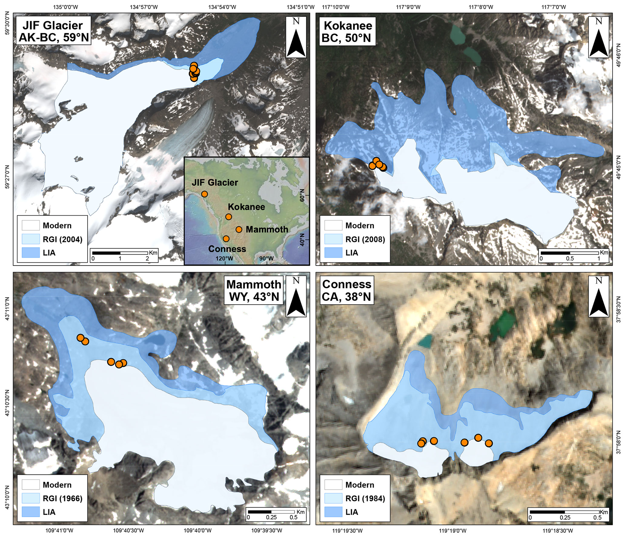
Figure 1 Study site locations and historical ice extents. Little Ice Age extent mapped from trimlines and moraines assumed to be last occupied by glaciers in ∼1880 CE. Proglacial bedrock sample locations from this study denoted by orange dots. Modern ice extent represents glacier size in 2021 CE. Randolph Glacier Inventory (RGI) date depends upon data availability in the RGI database. Image credit: © Copernicus.

Kokanee Glacier (49.75^∘ N, 117.14^∘ W, 2561 m) is in southeastern British Columbia in the Selkirk Mountains. Menounos et al. (2009) review Holocene glacier fluctuations in the Canadian Cordillera using lake sediment records, moraine dendrochronology, and lichen ages. They find that from 11–7 ka, ice was smaller than its extent in the late 20th century. Episodic glacier advances occurred at 8.6–8.1, 7.4–6.5, 5.8, 4.4–4.0, 3.7–2.8, 1.7–1.3 ka, and through the LIA (Menounos et al., 2009; Osborn et al., 2012). These advances are inferred to be synchronous at the centennial scale amongst the southern Canadian Cordillera, suggesting that these advances are related to broad climate signals across western North America (Menounos et al., 2009).

Mammoth Glacier (43.17^∘ N, 109.67^∘ W, 3627 m) is in the Wind River Range, Wyoming. Its Holocene length history is expected to follow that of the western United States and Canada: glaciers reached Holocene minimum positions between 11–7 ka and then advanced to maximum extents during the LIA (Marcott et al., 2019; Menounos et al., 2009). Distal lake sediment fluxes from the valley below Mammoth Glacier suggest that the glacier has been active since at least 4.5 ka – though perhaps disappearing in the Early Holocene – but was much smaller than its LIA extent from 4.5–1 ka (Davies, 2011), implying a substantial advance during the LIA.

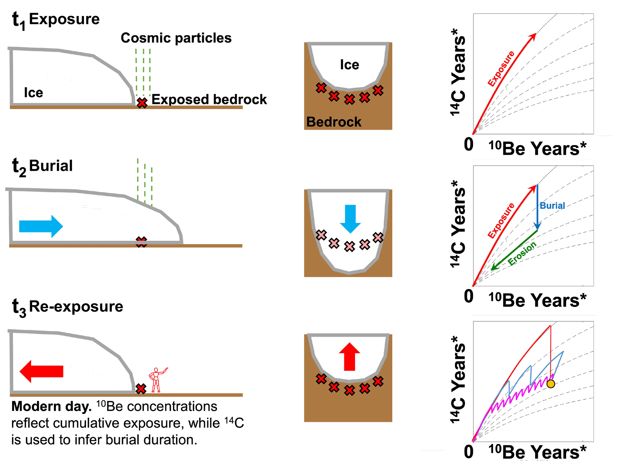
Figure 2 Schematic of in situ ¹⁴C–¹⁰Be concentrations in proglacial bedrock in response to glacier length fluctuations. At t₁, bedrock is exposed and nuclides accumulate along the continuous exposure curve. At t₂, the glacier has advanced and buried the bedrock. Nuclide production ceases while erosion occurs; ¹⁴C decays rapidly relative to ¹⁰Be during burial, while erosion removes both nuclides. At t₃, bedrock is re-exposed during modern retreat and sampled. Many scenarios of exposure, burial, and erosion can explain the measured nuclide concentrations, represented by the colored lines in the nuclide plot.

Conness Glacier (37.97^∘ N, 119.32^∘ W; 3603 m) is in the Sierra Nevada, California, USA. Glaciers in the Sierra Nevada are thought to have disappeared entirely by the Early Holocene (∼10 ka) prior to so-called “neoglacial” advances beginning at ∼3 ka (Bowerman and Clark, 2011; Cary, 2018; Konrad and Clark, 1998; Porter and Denton, 1967). Progressively increasing fluxes of rock flour from ∼3 ka to the LIA have been documented in distal lake sediments at Conness Glacier (Konrad and Clark, 1998) and at Palisade Glacier (Bowerman and Clark, 2011), located ∼125 km south of Conness Glacier, interpreted as the reformation and advance of both glaciers.

3 Methods

3.1 Field sampling, laboratory procedures, and cosmogenic nuclide concentration measurements

We collected surface exposure samples by hammer and chisel from glacially abraded, quartz-bearing bedrock within tens of meters of the modern ice margin. We targeted bedrock high points (local topographic maxima) as they are less likely to have prior till accumulation during episodes of exposure. We sampled abraded bedrock to minimize the chance that the bedrock had been quarried, although abrasion does not exclude the possibility of subglacial quarrying prior to abrasion (Rand and Goehring, 2019). All samples were collected in the last 5 years: JIF Glacier samples collected in 2019, Kokanee Glacier in 2018, Mammoth Glacier in 2020, and Conness Glacier in 2018. We present apparent exposure ages that are calculated using the CRONUS-Earth online calculator v.3 (Balco et al., 2008) with the LSDn scaling scheme (Lifton et al., 2014) and primary production dataset of Borchers et al. (2016). These ages assume continuous exposure with no erosion, modern elevation, and standard atmosphere. Uncertainties presented are analytical (i.e., internal, measurement) only. Exposure ages are “apparent” because subglacial erosion removes nuclides during burial, thus lowering the calculated exposure age from some “true” exposure age.

Quartz separation procedures are modified from Kohl and Nishiizumi (1992). We crushed and sieved samples (∼1 kg of rock) to the 250–710 µm size fraction, magnetically separated the minerals, and etched the non-magnetic fraction in dilute HCl and HF/HNO₃. We performed chemical froth flotation on these aliquots to remove feldspathic minerals. We etched remaining grains in dilute (1 %–5 %) HF/HNO₃ until pure quartz was attained. Samples were then wet-sieved at 250 µm to remove lingering mafic minerals, fine quartz grains, and partially dissolved feldspars. Quartz purity was confirmed by inductively coupled plasma optical emission spectroscopy (ICP-OES) measurement. Quartz was separated at Boston College for samples from Kokanee Glacier and Conness Glacier, at the University of Wisconsin-Madison for samples from Mammoth Glacier, and at Tulane University for samples from JIF Glacier.

We analyzed all samples for in situ cosmogenic ¹⁴C and ¹⁰Be concentrations. ¹⁰Be extraction procedures follow Ceperley et al. (2019). We extracted ¹⁰Be at the University of Wisconsin-Madison for all samples except JIF Glacier samples, which were extracted at Tulane University and follow procedures of Corbett et al. (2016). We spiked the samples with a ⁹Be carrier prepared from raw beryl (OSU White standard, 251.6±0.9 ppm; JIF Glacier samples TuBE, 904±28 ppm). We isolated Be from Fe, Ti, Al, and other ions using anion–cation exchange chromatography. We precipitated BeOH in a pH 8 solution and incinerated the BeOH gels at ∼1000 ^∘C to convert to BeO. We packed samples with Nb powder into stainless-steel cathodes for accelerator mass spectrometry analysis. ¹⁰Be $/$ ⁹Be ratios were measured at Purdue Rare Isotope Measurement Lab relative to 07KNSTD dilution series. We ran each batch with at least two blanks; we background-corrected samples using the average blank value from within the specific sample batch.

We extracted ¹⁴C at Tulane University for all samples following Goehring et al. (2019). ¹⁴C $/$ ¹³C ratios were measured at the National Ocean Sciences Accelerator Mass Spectrometry (AMS) facility. We calculated exposure ages using the CRONUS Earth-online calculator v.3 using LSDn scaling (Balco et al., 2008; Lifton et al., 2014). Exposure age calculations have ±4 % external uncertainty (Phillips et al., 2016).

3.2 ¹⁴C–¹⁰Be ratios as records of past glacier length

We determined the total time during the Holocene that each glacier was larger or smaller than its present-day size using in situ cosmogenic ¹⁴C–¹⁰Be dating of proglacial bedrock (Goehring et al., 2011). The bedrock abutting the terminus of a glacier today was exposed or buried during the Holocene as the glacier advanced and retreated over the bedrock (Fig. 2). We collected several ($n=\mathrm{5}-\mathrm{9}$) bedrock samples at the modern margin of each glacier that were recently exposed during modern retreat (Fig. 1). We assume that all samples at a given glacier experienced the same exposure–burial history because the samples have been exposed by retreating ice roughly contemporaneously (within uncertainties of cosmogenic nuclide dating). Nuclide concentrations vary amongst the samples in each glacier's transect due to unique erosion depths. Exposure duration is inferred from ¹⁰Be concentrations which accumulate when the glacier is smaller than its modern size; burial duration is inferred from disparity between ¹⁴C and ¹⁰Be concentrations because ¹⁴C ($t_{\mathrm{1}/\mathrm{2}}=\mathrm{5700}\pm \mathrm{30}$ years) decays rapidly during burial relative to ¹⁰Be ($t_{\mathrm{1}/\mathrm{2}}=\mathrm{1.387}\pm \mathrm{0.012}$ Myr; Chmeleff et al., 2010; Hippe, 2017). We assume that subglacial erosion during the last glacial period removed any nuclides from pre-Holocene exposure (Ivy-Ochs and Briner, 2014), consistent with the absence of cosmogenic exposure ages greater than the length of the Holocene measured in this study. We also assume that burial by till or nonglacial debris (e.g., rockfalls, hillslope sloughing) is insignificant. Although it is possible that bedrock sites were covered in debris during intervals of past ice recession, that scenario is unlikely to uniformly affect all samples given the spatial variability of such deposits, and thus coherency between samples is a reasonable check.

3.3 Monte Carlo forward model of nuclide concentrations in proglacial bedrock

We apply a Monte Carlo forward model of ¹⁴C and ¹⁰Be concentrations in proglacial bedrock (Vickers et al., 2020) to determine when in the Holocene each glacier was larger or smaller than its modern position. Because numerous combinations of bedrock exposure, burial, and erosion can create the same concentrations in bedrock, we use the Monte Carlo forward model to iterate through a list of 100 000 exposure–burial scenarios at various erosions rates to identify scenarios that reproduce nuclide concentrations within 2σ measurement uncertainty. Fundamentally, the model calculates the evolution of ¹⁴C and ¹⁰Be concentrations in a 5 m bedrock column as a glacier advances and retreats over the bedrock surface, simulating production during exposure, and decay and erosion when buried. Each sample is simulated one at a time, and scenarios that can explain the measurements made on all samples at a given glacier are considered successful. Below, the full details of the Monte Carlo forward model are provided; the original documentation can be found in the supplement to Vickers et al. (2020).

The Monte Carlo forward model is governed by Eq. (1):

$$\begin{array}{}\text{(1)}& N\left(z,t\right)=P_{\mathrm{NT}}\left(z\right)\cdot t+N\left(z,t-\mathrm{1}\right)\cdot e^{\left(-{\mathit{\lambda }}_N\cdot t\right)},\end{array}$$

where N is the concentration of the nuclide in the bedrock as a function of depth (z) and time (t), P_NT is the total production of the nuclide via spallation and muon production as a function of depth, and λ_N is the decay constant of the nuclide. The model simulates a binary between exposure or burial; no partial exposure or production through thin ice is considered (ice thicknesses >10 m make production negligible; Goehring et al., 2011). During exposure, nuclide production is simulated with depth according to CRONUS production and depth attenuation rates (Balco et al., 2008, left of the addition sign in Eq. 1), while radioactive decay is ongoing. During burial, production ceases and radioactive decay depresses ¹⁴C relative to ¹⁰Be (the right side of the addition sign in Eq. 1), while erosion is simulated by removing the top of the bedrock column at a prescribed rate. We assume that erosion only occurs during burial. Samples with ¹⁴C–¹⁰Be ratios above the production ratio for surface exposure are excluded from the Monte Carlo forward model as some of these samples are not physically reproducible (i.e., ratios cannot be recreated at any erosion depth from our Holocene erosion–burial scenarios), a decision explored in the Discussion.

To be consistent and to consider a range of possible Holocene histories, the Monte Carlo forward model tests the same 100 000 exposure–burial histories for each sample. Each scenario is discretized into 100-year time steps representing either exposure or burial, and there are 110 total time steps summing to 11 000 years. To generate a list of exposure–burial histories that are representative of all the possibilities (2¹¹⁰ possibilities, to be precise), one cannot simply select exposure or burial at random for any given time step, as this leads to highly oscillatory behavior where the state changes, on average, every time step. In correcting for this, we quasi-randomly generate scenarios by specifying the probability that one time step is the same as its preceding time step, designated the P value. For example, if P=0.50, there is a 50 % chance that a given time step has the same designation (exposure or burial) as the preceding one. Scenarios generated at P=0.5 have high-frequency variability, while scenarios generated at P=0.99 are relatively stable, typically with millennia of either exposure or burial at a time. The comprehensive list of 100 000 histories used in this paper was generated with constant P values between 0.6 and 0.99, increasing in increments of 0.01 (i.e., P=0.60, P=0.61, etc. to P=0.99 with 2500 histories per P value). We discounted P<0.6 because values below this threshold did not produce viable exposure–burial histories.

The nuclide concentrations at each sample location are forward modeled using erosion rates from 0.0–2.5 mm yr⁻¹ in steps of 0.1 mm yr⁻¹. A scenario is considered successful for a particular bedrock sample if the final surface ¹⁴C and ¹⁰Be concentrations are within uncertainty as determined by the 2σ measurement uncertainty and the production rate ratio uncertainty (7.3 % for ¹⁴C and 8.3 % for ¹⁰Be, 1σ; Borchers et al., 2016) added in quadrature. Scenarios that reproduce all nuclide concentrations for all samples at a given glacier are recorded and saved as viable exposure–burial histories; we henceforth refer to these as “overlapping” scenarios. Solutions that do not include burial in the final 200 years are discarded given the broad evidence of expanded glacier positions during the LIA (Solomina et al., 2015; Menounos et al., 2009) and satellite imagery showing most sample positions buried under ice until the last few years before sampling (Fig. 3).

We report the percentage of overlapping scenarios that have exposure at each time step as “probability of exposure” through time (Figs. 5; S5 in the Supplement). The probability of exposure is the percentage of overlapping scenarios that feature exposure at a given time step. For example, if 900 out of 1000 plausible exposure–burial scenarios include exposure from 8.1–8.0 ka, then the probability of exposure in that time step is 90 %. We interpret the change in probability of exposure from greater than 50 % to less than 50 % to indicate roughly when the glacier advanced past its modern position and buried the bedrock transect we sampled.

3.4 Glacier mapping, hypsometry, and response time

Although we are primarily concerned with length fluctuations of the four glaciers in the Holocene, our measurements are inherently linked to the modern-day position of each glacier because it is the reference point. It is therefore necessary to understand the history of each glacier's position since the industrial era that influenced its modern position. We first mapped modern (2021 CE) glacier area against LIA glacier extents in QGIS to characterize glacier retreat over this period (Fig. 1). We inferred the LIA glacier extents from moraines and trimlines. We overlaid glacier outlines onto modern satellite imagery from Copernicus. We also included an intermediate position using the outlines available from the Randolph Glacier Inventory (RGI Consortium, 2017). The amount of retreat since ∼1880 CE is related to the climate change at the glacier and the glacier's response time, defined as the time for each glacier's length to reach equilibrium with climate change. Hypsometric variables such as ice surface slope, cirque-wall shading, and debris cover impact response time, with steep ice surface slopes thought to be a particular correlate for quick response times (Pelto and Hedlund, 2001; Zekollari et al., 2020). We approximate each glacier's response time according to Jóhannesson et al. (1989), where mean glacier thickness is divided by maximum mass loss from the terminus as shown in Eq. (2):

$$\begin{array}{}\text{(2)}& \mathit{\tau }={\displaystyle \frac{H}{-b_{\mathrm{t}}}},\end{array}$$

where τ is the time for volume adjustment in years, H the thickness in meters (m), and b_t the maximum mass loss at the terminus (in m yr⁻¹). Mean glacier thickness is taken from Farinotti et al. (2019), and maximum mass loss at the terminus is from Hugonnet et al. (2021). This approximation for response time (along with glacier slope) provides insight into the glacier's response to industrial-era warming. We note this calculation is a minimum estimate of how quickly a glacier could adjust its volume because we use the maximum mass loss from the terminus; the purpose of this calculation is merely to serve as a common point of comparison amongst the four glaciers rather than a robust estimate of glacier response time. We present glacier areas in Fig. 6 and report all glacier hypsometry data and response time calculation details in Table 2.

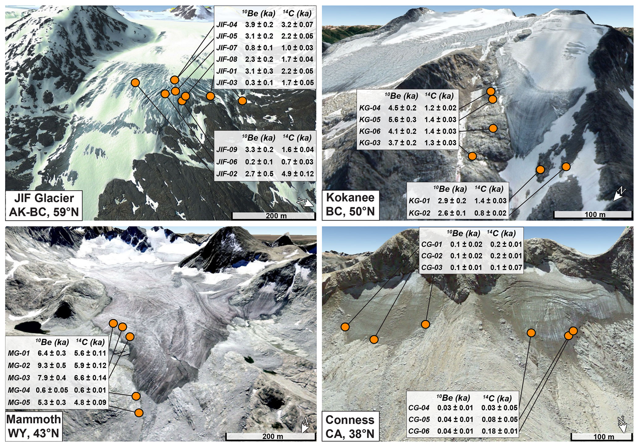
Figure 3 Oblique satellite images of glacier forefields with sample locations and apparent ¹⁴C and ¹⁰Be exposure ages (CRONUS). Sample locations denoted by colored dots corresponding to each glacier. Images are from different years; the highest-resolution years with least snow cover were selected. Some samples are still buried by glacial ice at the time the image was captured, showing the recent burial prior to sampling in 2018–2020 CE. Image years: Juneau Icefield Glacier, 2011; Kokanee Glacier, 2021; Mammoth Glacier, 2006; and Conness Glacier, 2013. Image credit: © Google Earth.

4 Results

4.1 ¹⁴C–¹⁰Be ratios, burial isochrons, and exposure ages

Apparent exposure ages are presented in Table 1 and plotted onto satellite imagery of the glacier forefields in Fig. 3. The highest ¹⁰Be ages likely have experienced the least erosion during burial and thereby provide an approximate sense for total Holocene exposure. We therefore calculated the mean and standard deviation of the three highest apparent ¹⁰Be ages at each glacier. The first observation is that ¹⁰Be bedrock exposure ages are non-uniform across the four glaciers: mean ¹⁰Be exposure ages are the highest at Mammoth Glacier of the four sites, with a mean from the three highest apparent exposure ages of 7.9±1.5 ka; Kokanee Glacier bedrock has the next-highest apparent ¹⁰Be exposure ages, with an average of 4.7±0.8 ka from its three most-exposed samples; JIF Glacier bedrock has a mean ¹⁰Be age 3.4±0.4 ka of its three highest ages; and Conness Glacier bedrock has a mean ¹⁰Be age of 0.1±0.02 ka for its three highest measurements.

We then plotted our results as nuclide ratios along exposure and burial isochrons (Fig. 4). The burial isochrons leverage the preferential decay of ¹⁴C to provide approximate insight into Holocene burial durations. Nuclide concentrations have been normalized by their local production rates to easily compare between sites (such that concentrations are expressed in years). The solid line represents ¹⁴C–¹⁰Be ratios under continuous exposure. The dashed lines represent ¹⁴C–¹⁰Be ratios when bedrock is buried, and the ¹⁴C–¹⁰Be ratios are depressed through the relatively rapid decay of ¹⁴C. Figure 4 does not include any erosion, though samples plotting closer to the origin but along the same isochron are typically more eroded than those further from the origin. Glacial erosion less than 2 m depth removes both nuclides in roughly equal proportions, such that ¹⁴C–¹⁰Be ratios are not significantly altered (Hippe, 2017).

Table 1 ¹⁴C and ¹⁰Be concentrations and apparent exposure ages. All uncertainties are 1σ and internal only.

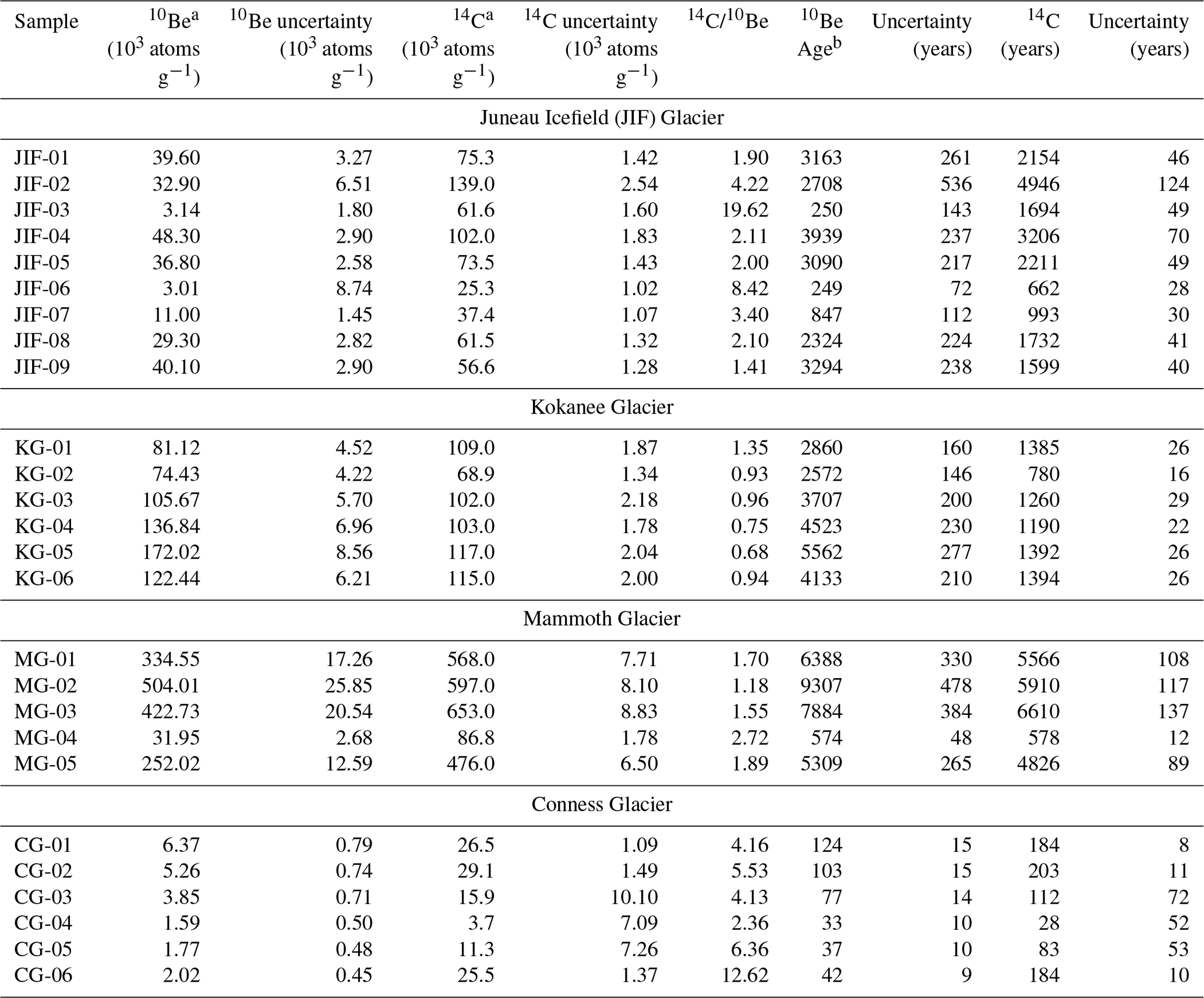
^a Nuclide concentrations are blank-corrected specific to each sample batch. See the Supplement for background measurements. All AMS measurements are standardized to 07KNSTD. ^b Calculated using the CRONUS-Earth online calculator v.3 (Balco et al., 2008) with the LSDn scaling scheme (Lifton et al., 2014).

The second observation is that ¹⁴C–¹⁰Be sample ratios at JIF Glacier, Kokanee Glacier, and Mammoth Glacier are depressed relative to the production ratio, which is indicative of exposure followed by burial via the rapid decay of ¹⁴C relative to ¹⁰Be (Fig. 4). Like the apparent exposure ages, nuclide ratios from the four glaciers appear distinct, with the samples from each glacier plotting in separate regions of the isochron plot. The Mammoth Glacier samples cluster around 1–2 kyr of burial. These samples have high ¹⁴C–¹⁰Be ratios, which are only possible with minimal burial (otherwise ¹⁴C concentrations would be lower). Bedrock samples from Kokanee Glacier have the lowest ¹⁴C–¹⁰Be ratios of any of the four sites and suggest Holocene burial durations of 6–10 kyr. Low ratios are only possible through extensive decay of ¹⁴C relative to ¹⁰Be, severely constraining the plausible exposure–burial scenarios. The JIF Glacier samples have two populations: samples below the continuous exposure curve and samples above the continuous exposure curve. Of the samples beneath the continuous exposure curve, four samples plot at ∼2–3 kyr of burial. These four samples plot closer to the origin than the Mammoth Glacier bedrock despite similar burial durations, suggesting the JIF Glacier samples are more deeply eroded. The samples above the continuous exposure curve are difficult to interpret, which we consider in the Discussion. The Conness Glacier samples have uniquely low nuclide concentrations amongst the four glaciers – approaching AMS-system blank levels – and are clustered around the origin. Low nuclide concentrations reflect burial for thousands of years, either by glacial ice, bedrock that was eroded away, or debris.

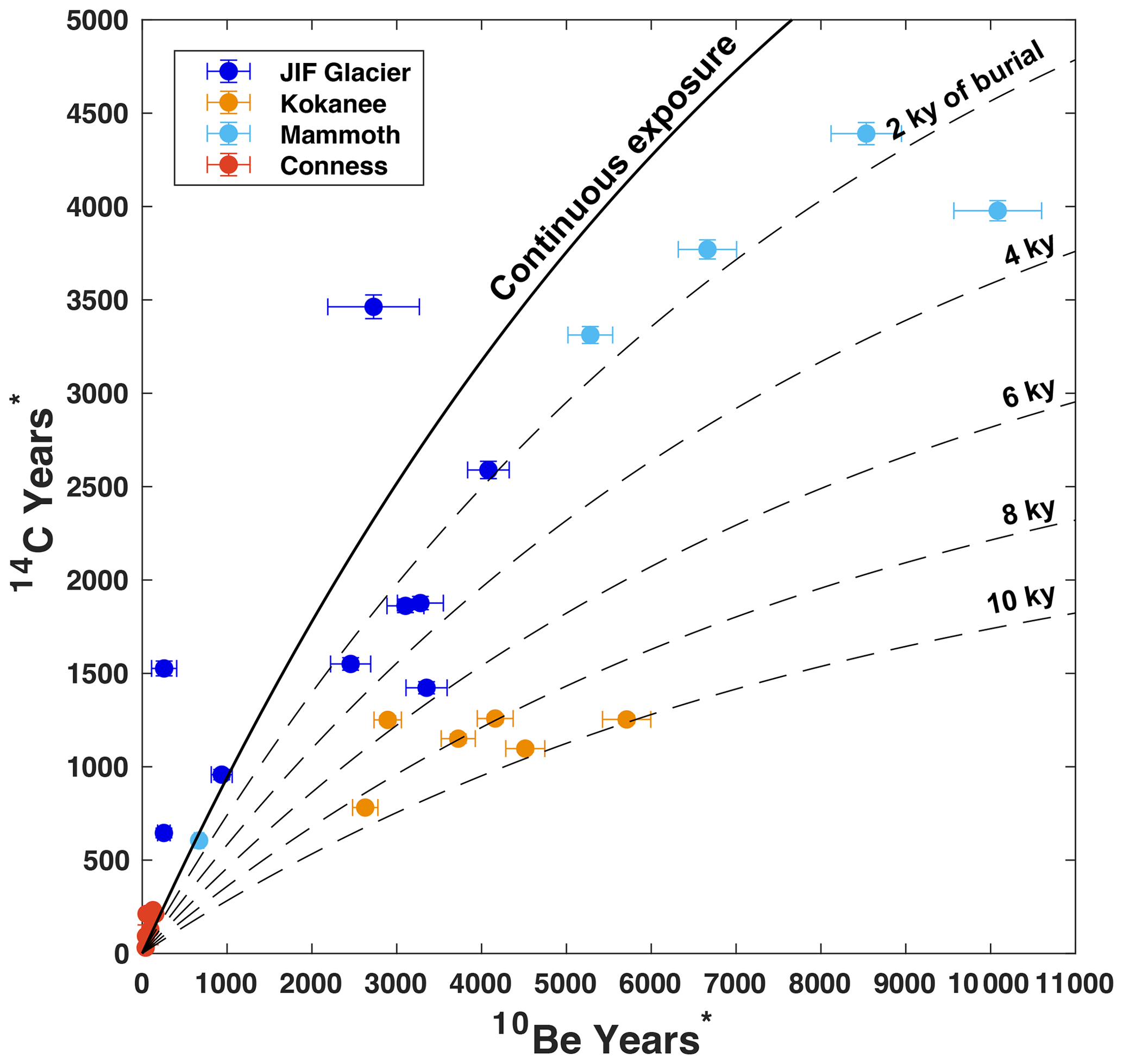
Figure 4 ¹⁴C–¹⁰Be ratios plotted against burial isochrons. Nuclide concentrations are normalized by their local production rates. The solid line represents the evolution of ¹⁴C–¹⁰Be ratios if samples are continuously exposed. Subsequent dashed lines represent ¹⁴C–¹⁰Be ratios when sample bedrock is buried, and the ¹⁴C–¹⁰Be ratio is depressed through radioactive decay. The x axis approximates integrated exposure during the Holocene in years, while the y-axis values inform burial duration.

4.2 Holocene exposure–burial histories and erosion rates from Monte Carlo forward modeling

We present the results from the Monte Carlo forward model experiments separately from the nuclide ratios, so the two methods can be compared. We plotted the overlapping exposure–burial scenarios as bedrock “probability of exposure” through the Holocene (Fig. 5). The full model output with plausible exposure–burial histories for each sample and a histogram of the erosion rates used at each sample can be found in Figs. S5 and S6.

The Monte Carlo forward model results predict that JIF, Kokanee, and Mammoth glaciers were smaller than their modern size in the Early-to-Mid-Holocene and larger than their modern size in the Late Holocene (Fig. 5). At Mammoth Glacier, bedrock shows the most exposure of the four sites (from 11–1 ka) and the latest burial in the Holocene (∼1 ka). The number of overlapping scenarios is 124. The probability of exposure is relatively high (80 %–90 %) during inferred exposure, suggesting good agreement amongst the overlapping scenarios. Kokanee Glacier exhibits exposure before ∼6 ka and burial after ∼6 ka. The number of plausible overlapping scenarios is 137. The overlapping scenarios for Kokanee's bedrock similarly agree well with each other: the probability of exposure is >90 % in the Early Holocene and <10 % by 5 ka. At JIF Glacier, model results suggest bedrock burial at ∼2 ka. The number of plausible overlapping scenarios is 282. However, the probability of exposure at any one time is relatively low, never rising above 70 %.

We calculated the mean erosion rates used in only the overlapping scenarios from each glacier and plot the data as histograms in Fig. S7. This includes all samples to provide an approximate erosion rate at a given glacier. The mean erosion rate at Mammoth Glacier is 0.7±0.7 mm yr⁻¹ (0.2±0.2 mm yr⁻¹ when a low-concentration sample is excluded, see Discussion), 0.04±0.03 mm yr⁻¹ at Kokanee Glacier, and 0.3±0.3 mm yr⁻¹ at JIF Glacier.

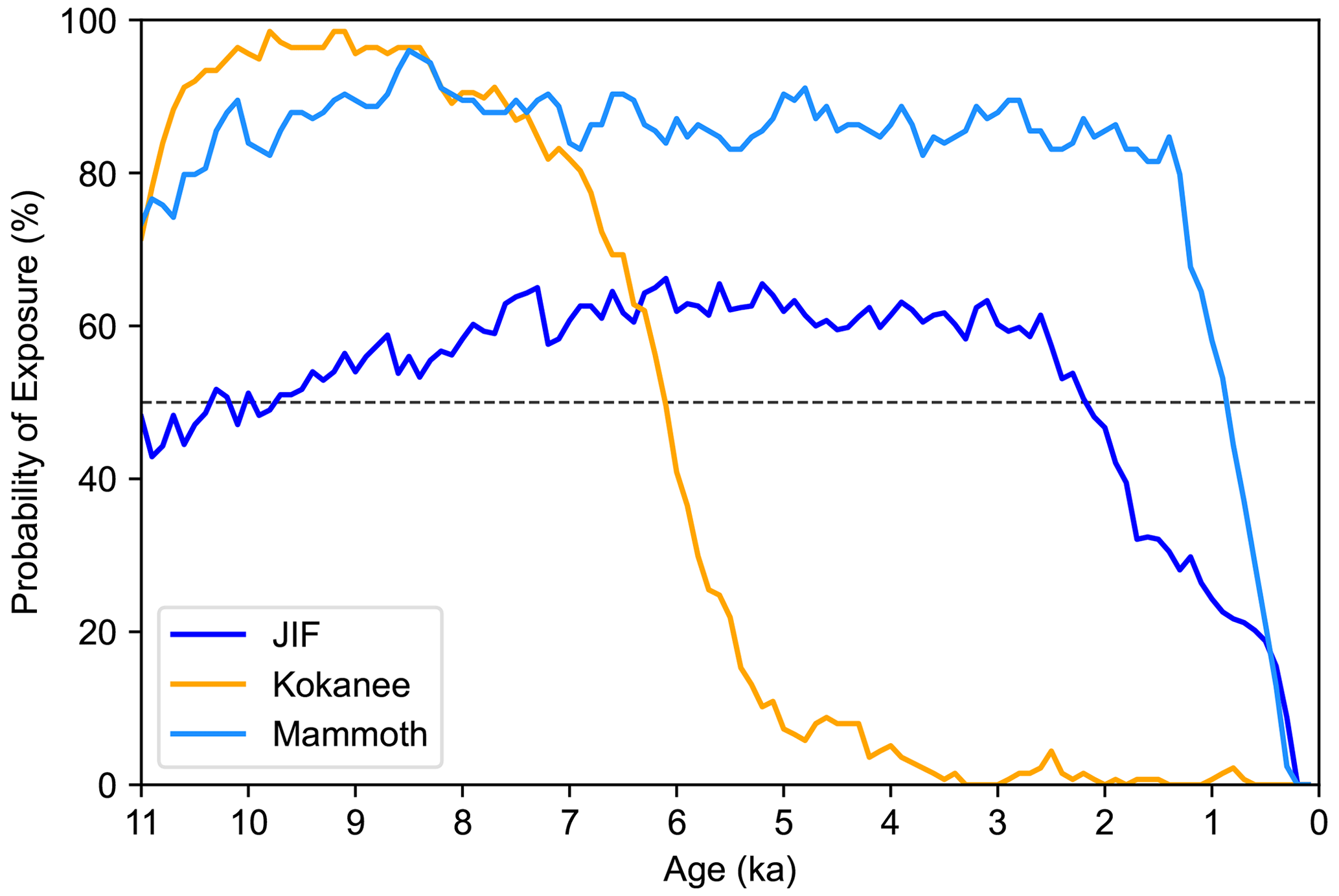
Figure 5 Modeled probability of exposure of bedrock at Juneau Icefield, Kokanee, and Mammoth glaciers from Monte Carlo forward model results. Probability of exposure is generated from overlapping scenarios between all samples at a given glacier. The change in probability of exposure from greater than 50 % to less than 50 % indicates roughly when the glacier advanced past its modern position. Results from Conness Glacier are not presented here; see Fig. S8 for Monte Carlo forward model output.

Nuclide concentrations in the Conness Glacier samples are uniquely low amongst the four glaciers, which poses challenges for our Monte Carlo analysis. At such low concentrations, small differences in blank corrections, scaling schemes, and production pathways have an outsize influence on modeling nuclide concentrations. We initially ran the model using the same parameterizations at the other sites where erosion rates are tested up to 2.5 mm yr⁻¹. The model finds 4914 overlapping solutions, and erosion rates skew heavily towards the highest possible rates (2.5 mm yr⁻¹; Fig. S8). However, erosion rates at the other three sites all skew towards lower rates (<0.5 mm yr⁻¹; Fig. S6), and there is no geologic evidence that Conness Glacier is a uniquely erosive glacier. We then re-ran the Monte Carlo forward model with erosion rates capped at 0.5 mm yr⁻¹. Under this low-erosion parameterization, no scenarios could reproduce the measured concentrations at all samples (zero overlapping scenarios, Fig. S8). Because of these complexities, we do not present modeling results from Conness Glacier in Fig. 5 and explore the various ways to interpret the low concentrations in the Discussion.

4.3 Glacier mapping, hypsometry, and response time calculations

The four glaciers retreated 14 %–70 % from their maximum Holocene extents recorded during the LIA (Fig. 6). We also present intermediate glacier positions where available from the published literature and composite data calculated for the Wind River Range and the Sierra Nevada to provide insight into how each glacier compares to the rest of the glaciers in its region (Basagic and Fountain, 2011; DeVisser and Fountain, 2015).

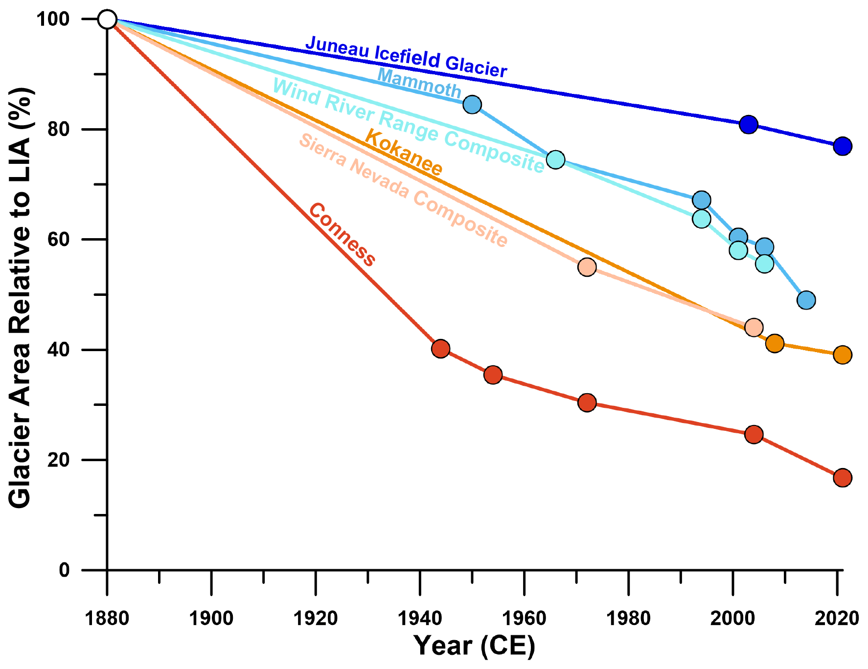
Figure 6 Glacier area through the industrial era relative to glacier area at the end of the Little Ice Age (LIA). LIA moraines assumed to be last occupied at ∼1880 CE (Menounos et al., 2009; Wanner et al., 2008). Two composites of regional glaciers from the Wind River Range and Sierra Nevada are included to provide context for regional glacier change (DeVisser and Fountain, 2015; Basagic and Fountain, 2011). Internal mapping has been supplemented with mapping by DeVisser and Fountain (2015) at Mammoth Glacier and Basagic and Fountain (2011) at Conness Glacier. See Table S5 for calculation and source details.

Conness Glacier is 14 % of its LIA area; it is the most retreated of the four glaciers relative to its LIA area. It has also retreated more than the composite of Sierra Nevada glaciers (Fig. 6). Kokanee Glacier has retreated the second-most, occupying 46 % of its LIA area today. Mammoth Glacier is 49 % of its LIA area; its retreat closely matches the average retreat for glaciers in the Wind River Range. JIF Glacier has retreated the least and is 70 % of its LIA area.

Glacier hypsometry data and response time calculations are presented in Table 2. The four glaciers can be subdivided into two groups: (i) bigger glaciers with shallow ice-surface slopes and slow response times and (ii) smaller glaciers with steep ice-surface slopes and quick response times. JIF Glacier and Mammoth Glacier are characterized by their shallow slopes and slow response times. JIF Glacier has the shallowest ice surface (5^∘) and the longest response time (τ=27 years) of the four glaciers. It is also the largest glacier studied here, with an area of 15.2 km² in 2021 (compared to the smallest glacier presented, Conness Glacier, at 0.1 km²). Mammoth Glacier has the second-shallowest ice-surface slope at 9^∘ and the second-slowest response time (τ=23 years). Kokanee Glacier and Conness Glacier are characterized by their relatively steep slopes and quick response times. Kokanee Glacier has a steep ice-surface slope at 22^∘ and the second quickest response time (τ=14 years). Conness has the steepest ice surface slope, 23^∘, suggesting the quickest response time of the glaciers studied here given the relationship between slope and response time proposed by Zekollari et al. (2020). We omit Conness Glacier from these calculations because there was a large discrepancy between the area of the glacier today and the area of the glacier used in the mean thickness calculations by Farinotti et al. (2019).

Table 2 Glacier hypsometry data.

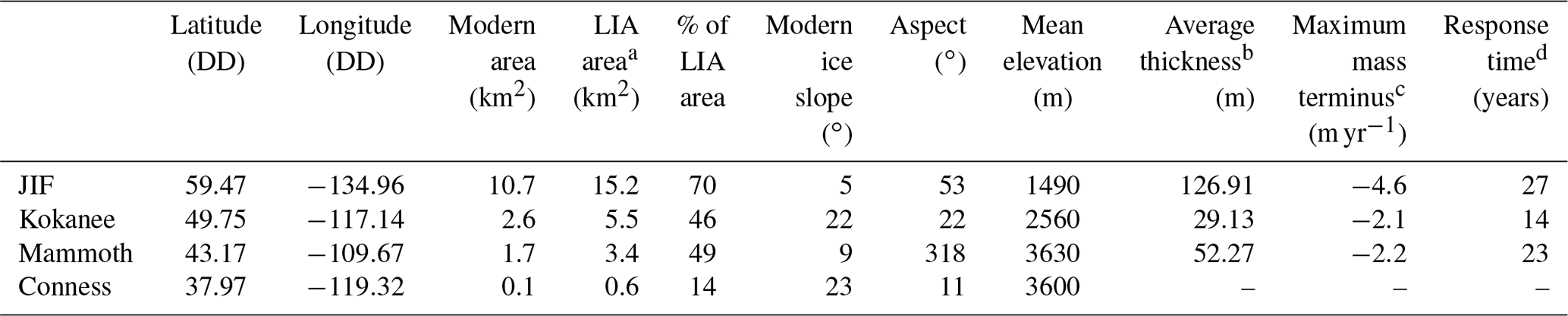
^a Little Ice Age areas were mapped for this study based on trimline and proximal moraines as seen in Fig. 1. ^b From Farinotti et al. (2019). ^c From Hugonnet et al. (2021). ^d Calculated according to Jóhannesson et al. (1989). Conness Glacier omitted due to large discrepancies between ice extent when calculations were made versus modern ice extent.

5 Discussion

In agreement with broad evidence of Holocene glacier advance in western North America (Menounos et al., 2009; Solomina et al., 2015; Davis et al., 2009), our results at three of four sites suggest glaciers advanced past their modern positions in the Mid-to-Late Holocene. The trend is apparent from the nuclide ratios alone: sample populations from JIF Glacier, Kokanee Glacier, and Mammoth Glacier all exhibit the depressed ¹⁴C–¹⁰Be ratios characteristic of Early-to-Mid-Holocene exposure followed by Late Holocene burial. At Conness Glacier, ice growth cannot be inferred due to near-blank nuclide concentrations, although it seems likely given the evidence for increasing rock flour in the Sierra Nevada in the Late Holocene (Konrad and Clark, 1998; Bowerman and Clark, 2011). Mid-to-Late Holocene glacier expansion agrees with similar studies using in situ ¹⁴C–¹⁰Be to constrain glacier advance in the Swiss Alps, Peru, and Uganda (Goehring et al., 2011; Schimmelpfennig et al., 2022; Vickers et al., 2020). Minimum positions in the Early to Mid-Holocene supports the presence of a Holocene Thermal Maximum in western North America that remains persistent in proxy temperature records (Kaufman and Broadman, 2023), at odds with recent data-assimilation research that finds slight warming in the Holocene (Osman et al., 2021). Sea-surface temperature reconstructions from 30–90^∘ N (Marcott et al., 2013) and terrestrial temperature reconstructions from western North America (Routson et al., 2021) resemble decreasing Northern Hemisphere summer insolation (Fig. 7). Increasing winter precipitation (Routson et al., 2021) also likely contributes to glacier growth. Whether the observed glacier expansion is due to glaciers' seasonal bias is unclear, but our results support the proxy data trends of cooler summers and wetter winters.

Where we find our results surprising, however, is in the non-uniform bedrock burial durations. The ¹⁴C–¹⁰Be sample ratios and modeled exposure–burial histories suggest the glaciers advanced past their modern sizes thousands of years apart. Consider the two endmembers: Mammoth Glacier was likely smaller than its modern size for almost the entire Holocene until the last millennium, while Conness Glacier was larger than its modern size for the entire Holocene until present. These are vastly different Holocene length histories relative to their terminus positions today, despite evidence that western North America experienced roughly similar climate changes over the Holocene (Shuman and Marsicek, 2016; Menounos et al., 2009). Below, we first evaluate the modeled probabilities of exposure and compare them with the ¹⁴C–¹⁰Be ratios and extant paleoclimate data. Then, we explore hypotheses for why the modern glacier terminus positions are non-uniform relative to their Holocene length histories and their implications.

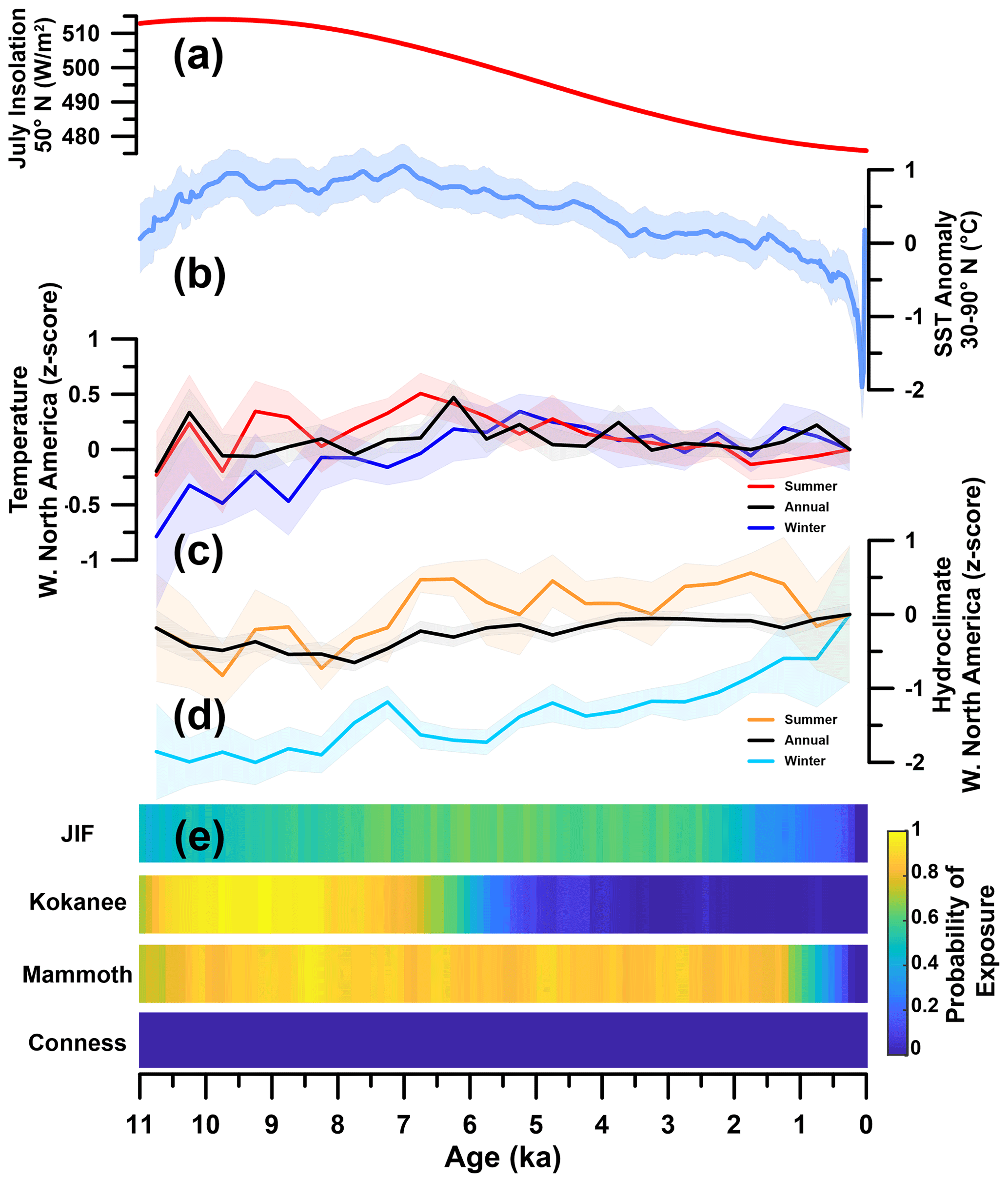
Figure 7 Holocene paleoclimate data and modeled probability of exposure at each glacier. (a) The 50^∘ N July insolation (Laskar et al., 2004). (b) Sea-surface temperature proxy reconstruction for 30–90^∘ N, where the shaded band is 1σ uncertainty (Marcott et al., 2013). (c, d) Annual and seasonal temperature and hydroclimate reconstruction from western North America proxy data (Routson et al., 2021). Temperature and hydroclimate indexes are relative to pre-industrial values, with more positive values being warmer and wetter and negative values colder and drier. (e) Modeled probability of exposure for each glacier. Color bar ranges from 100 % chance of exposure in yellow to 0 % chance of exposure (i.e., burial) in blue.

5.1 Holocene exposure–burial histories at each glacier

We first evaluate Mammoth Glacier and Kokanee Glacier because they appear to have tightly constrained Holocene exposure–burial histories. The high apparent exposure ages of both nuclides in the Mammoth Glacier samples require the glacier to be smaller than its modern area for most of the Holocene. The Monte Carlo forward model results quantify this interpretation, predicting Mammoth Glacier was smaller than its modern area from ∼11–1 ka before advancing beyond its modern position in the last millennium. An interesting implication therein is that Mammoth Glacier doubled in area in less than a millennium: at ∼1 ka the glacier's area was 1.7 km² and at ∼0.1 ka (end of the LIA) it was 3.4 km². This finding agrees well with the evidence from distal lake sediment cores that Mammoth Glacier was much smaller than its LIA extent from 4.5–1 ka and advanced significantly after 1 ka (Davies, 2011).

Sample MG-04 has exposure ages an order of magnitude lower (¹⁰Be: 0.5±0.05 ka, ¹⁴C: 0.6±0.01 ka) than the other samples in the Mammoth transect. The Monte Carlo forward model erosion rate histogram (Fig. S6) shows that much higher erosion rates are required for MG-04 than the other samples. Subglacial quarrying is a plausible mechanism for much deeper erosion at one point than others (Rand and Goehring, 2019). We interpret that this sample was deeply eroded, probably by quarrying, while the remaining samples are abrasion-dominated. We therefore present two erosion rates from Mammoth Glacier. With MG-04 included, the mean erosion rate is 0.7±0.7 mm yr⁻¹. With MG-04 excluded, the mean erosion rate is 0.2±0.2 mm yr⁻¹; we consider this more likely to represent an abrasion rate rather than a general erosion (quarrying-included) rate. We plot histograms for both distributions in Fig. S7.

Kokanee Glacier was smaller than its modern position from ∼10–6 ka and larger from ∼6 ka to the LIA. The tight convergence in the overlapping scenarios supports this interpretation. Kokanee Glacier samples have the lowest ¹⁴C–¹⁰Be ratios of the four glaciers (Table 1), which agrees with the longest burial duration inferred by forward modeling. The advance of Kokanee Glacier across its modern size threshold at ∼6 ka is earlier in the Holocene than any other site studied using the same sampling approach (Vickers et al., 2020; Goehring et al., 2011), but in good agreement with lake and moraine records that document glacier advances in Canada as early as 7 ka (Menounos et al., 2009). Our results imply that Kokanee has been larger than its present-day position today from ∼6 ka through the LIA and that any glacier length fluctuations from ∼6 ka onwards were between the position occupied at ∼6 ka and its LIA maximum extent. Erosion rates at Kokanee Glacier are quite low (0.04±0.03 mm yr⁻¹, Fig. S7). We interpret this erosion rate as better approximating an abrasion rate than a general erosion rate, since we avoided sampling surfaces that appeared plucked and there is no evidence for anomalously deep erosion in the data.

At JIF Glacier, the scatter in nuclide ratios and the relatively low agreement amongst overlapping scenarios make it challenging to infer a conclusive Holocene exposure–burial history. For one, it is difficult to interpret the samples that plot above the exposure curve in Fig. 4 (JIF-02, JIF-03, JIF-06, JIF-07). Deep glacial erosion (>2 m erosion depth) via subglacial quarrying has been hypothesized to explain ¹⁴C–¹⁰Be ratios that plot above the continuous exposure curve (Rand and Goehring, 2019). Radiocarbon has a higher muogenic production rate than ¹⁰Be such that, at some depth, the production ratio of ¹⁴C–¹⁰Be exceeds the surface production ratio. Glaciers in the Juneau Icefield are fed by high amounts of precipitation, which has been associated with high erosion rates (Cook et al., 2020), and Alaskan glaciers are generally considered to be some of the most erosive in the world (Koppes and Montgomery, 2009). If deep erosion is the cause of the elevated ¹⁴C–¹⁰Be ratios, then it should be replicable by modeling.

To explore the possibility of deep glacial erosion as the cause of samples plotting above the continuous exposure curve, we modeled simple Holocene exposure–burial histories at various erosion rates to explore the three-parameter space (Fig. 8). We modeled 10 simple histories: 9 kyr of exposure followed by 1 kyr of burial, 8 kyr of exposure followed by 2 kyr of burial, and so on to 1 kyr of exposure followed by 9 kyr of burial. These scenarios are applied to theoretical 5 m bedrock columns using the same production and depth attenuation code as the Monte Carlo forward model. We used a singular production rate created by averaging latitude, longitude, sample thickness, and elevation from all nine samples for simplicity. Then, we modeled the nuclide concentrations in each scenario at erosion rates (during burial) of 0.0–2.5 mm yr⁻¹, marked by vertical red tick marks along each scenario. Erosion rates in each scenario start at 0.0 mm yr⁻¹ on the righthand side. Erosion rates increase towards the origin, with erosion rates >1.0 mm yr⁻¹ clustering so tightly towards the origin that they are largely obscured on the plot.

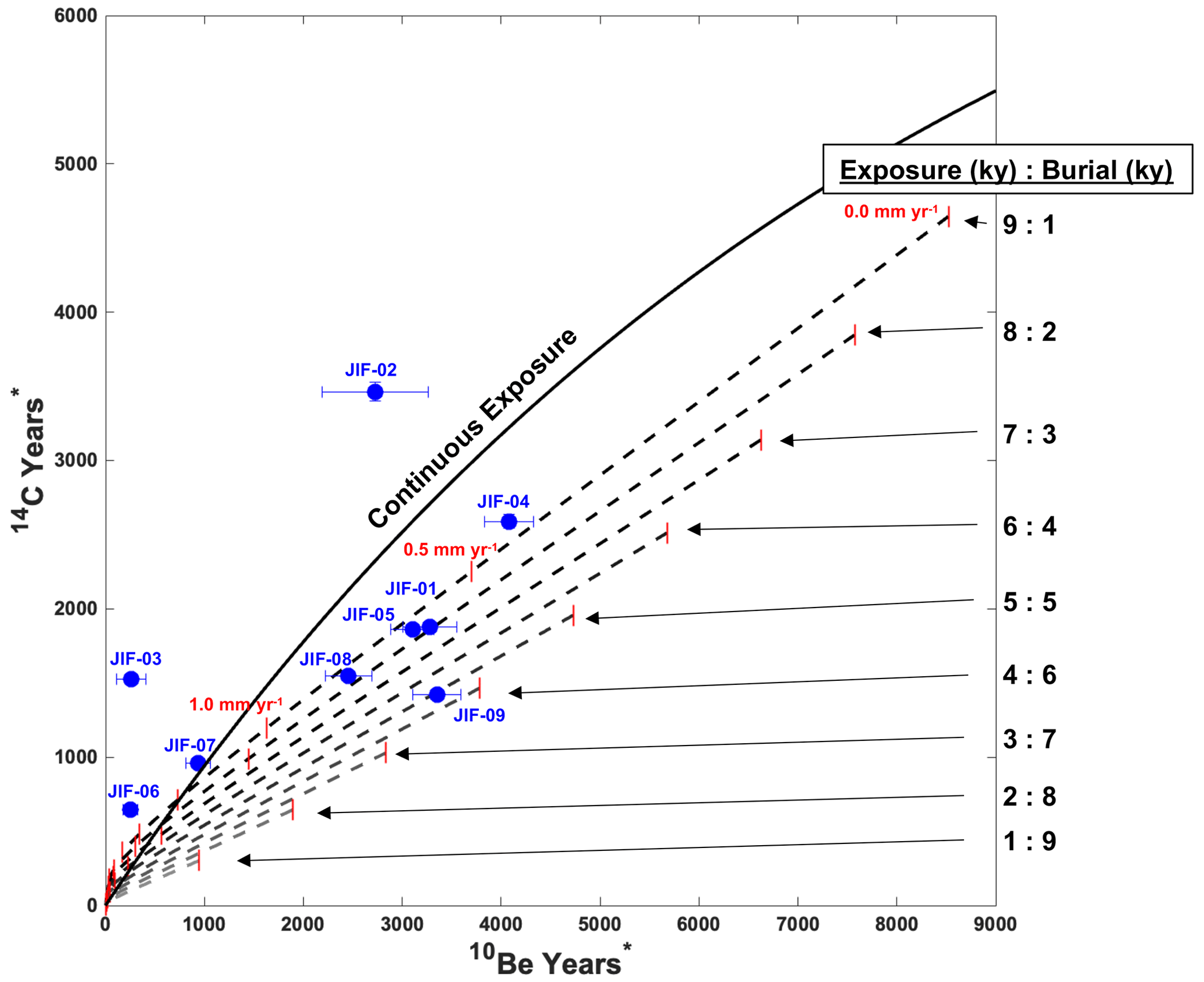
Figure 8 JIF Glacier ¹⁴C–¹⁰Be concentrations plotted against 10 “simple” Holocene exposure–burial scenarios along erosion isochrons. The solid line is continuous exposure (10 kyr of exposure with 0 year of burial), and dashed lines are subsequent exposure–burial scenarios labeled on the righthand side. Erosion rates are marked by red vertical tick marks along each scenario (black dashed line), starting from an erosion rate of 0.0 mm yr⁻¹ on the righthand side progressing to 2.5 mm yr⁻¹. As an example, erosion rates of 0.0, 0.5, and 1.0 mm yr⁻¹ are labeled in the first scenario. Concentrations have been normalized by their production rate such that concentrations are expressed in years.

There is only a small area towards the origin in Fig. 8 where deep erosion exhumes bedrock with ¹⁴C–¹⁰Be ratios above the continuous exposure curve (where the dashed lines are above the continuous exposure curve). Samples JIF-02 and JIF-03 are far outside of this region within measurement uncertainty (1σ); we exclude these samples as outliers since they are not physically reproducible. Samples JIF-06 and JIF-07 are close to this region but still outside of it within measurement uncertainty. These two samples may well be deeply eroded by quarrying, but it is not clear from our simple modeling exercise. These samples also were excluded from the Monte Carlo forward model simulations because no overlapping scenarios were found when they were included. For simplicity, we exclude all four of these samples from our interpretations and erosion rate calculations. This decision removes samples that may have been deeply eroded by quarrying, which means that the erosion rate from JIF Glacier is a minimum estimate that more likely approximates an abrasion rate than a general erosion rate.

Of the samples beneath the exposure curve in Fig. 8, samples JIF-01, JIF-05, and JIF-08 have relatively tight agreement along the scenario of ∼8 kyr of exposure followed by ∼2 kyr of burial at erosion rates of 0.3–0.4 mm yr⁻¹. These measurements also agree well with the burial durations suggested in Fig. 4, the timing of burial in the Monte Carlo forward model from ∼2 ka to present, and the mean erosion rate found from Monte Carlo forward model results (0.3 mm ±0.3 yr⁻¹). Samples JIF-04 and JIF-09 plot along different exposure–burial histories; this could be due to several geologic reasons such as partial shielding (snow, thin ice) or non-contemporaneous burial. Acknowledging the scatter in the dataset, the consistency of JIF-01, JIF-05, and JIF-08 across the modeling exercises appears to provide the simplest explanation. We therefore interpret that JIF Glacier was smaller than its modern position from ∼10–2 ka and larger from ∼2 ka to present but with less confidence than the findings from Mammoth and Kokanee. This interpretation agrees with findings from Clague et al. (2010) that show similar advances past modern margins at ∼2 ka by two outlet glaciers of the Juneau Icefield.

The extremely low nuclide concentrations at Conness Glacier could be explained by (1) glacial burial in the Holocene until modern retreat, (2) deep erosion, or (3) burial by debris when bedrock would otherwise be exposed during glacier retreat. We consider it unlikely that deep erosion is the primary explanation for the low concentrations. First, the Monte Carlo forward model experiments at various erosion rates are used to investigate deep erosion as a cause for the low concentrations. In the deep erosion scenarios, exposure is more likely in the Late Holocene (Fig. S8) than the Early Holocene, which is at odds with the understanding of Holocene glacier history in western North America. Second, the deep erosion scenario requires erosion rates at Conness to be higher than the other three sites, more so than even JIF Glacier, which has a mean thickness of over 100 m today and an area an order of magnitude larger (Table 2). A third line of evidence is the consistency of the measurements. Subglacial erosion via abrasion or quarrying is spatially variable; abrasion rates vary across the glacier valley (Goehring et al., 2011), while quarrying (the most plausible mechanism for rapid, deep erosion) is related to pre-existing bedrock fractures (Woodard et al., 2019). The measured concentrations at Conness Glacier are consistent and clustered tightly around the origin of the isochron plot (Fig. 4). Estimates in the literature of subglacial abrasion rates at mid-latitude glaciers vary widely, from 0.1 mm yr⁻¹ (Goehring et al., 2011; Schimmelpfennig et al., 2022) up to 5 mm yr⁻¹ (Wirsig et al., 2017), so although we cannot fully reject the deep erosion hypothesis, it seems unlikely. If not erosion, another possibility is that talus and debris falling off the cirque headwall may have covered the bedrock sites after deglaciation, preventing nuclides from accumulating prior to Late Holocene glacier reformation. Again, the consistency of the nuclide measurements is difficult to reconcile with the spatial heterogeneity of a talus field, and the burial would need to have happened immediately after deglaciation to keep concentrations near blank levels. While this hypothesis also cannot be completely rejected, it requires an unlikely set of conditions.

The simplest explanation for the extremely low nuclide concentrations is that Conness Glacier has buried the sample sites for the duration of the Holocene. Without erosion rates >0.5 mm yr⁻¹, there are no overlapping scenarios with exposure from our Monte Carlo forward model, and the modeled probability of exposure is “0 %” (Fig. 7). This finding challenges previously published work that projects glacier disappearance in the Sierra Nevada from 10–3 ka prior to “neoglacial” advance in the Late Holocene (Bowerman and Clark, 2011; Konrad and Clark, 1998; Porter and Denton, 1967). Whether Conness Glacier is representative of the entire Sierra Nevada or not remains an open question. It has retreated more by percentage of its LIA area than the composite of Sierra Nevada glaciers (Basagic and Fountain, 2011, Fig. 6) and the most amongst the four glaciers considered here. It therefore could be an outlier in the Sierras, outpacing other glaciers in its retreat. It is also possible that the hypsometry of Conness Glacier (e.g., headwall shading, orientation, insulation from debris) caused it to be resilient in the Early to Mid-Holocene, while others in the Sierra Nevada disappeared. The sensitivity of small glaciers like Conness to changes in temperature and precipitation has been shown to be similar to that of large glaciers, but small glaciers have been shown to be more variable from one to another than large glaciers (Huss and Fischer, 2016). Further research is needed to assess whether Conness Glacier is representative of the Sierra Nevada or an outlier, as well as to continue to probe hypotheses about the role of erosion and debris burial.

5.2 Understanding the non-uniform signal

We seek to understand why four North American glaciers would advance beyond their modern positions many thousands of years apart despite presumed common climate forcing over the Holocene and through the industrial era. While there is spatial climate variability over the Holocene, it seems unlikely that within western North America there would be variation large enough to cause the four glaciers to advance past their modern positions thousands of years apart. However, sufficient local terrestrial archives are lacking to determine if climate variability is the main driver of the spatial difference in our observed glacier changes (Routson et al., 2021). Therefore, we turn to the reviews of Holocene glacier change in western Canada (Menounos et al., 2009) and Holocene temperature and precipitation variability in North America (Shuman and Marsicek, 2016). These reviews suggest synchronicity across the region during the Holocene on centennial-to-millennial scales, rather than variability. Additionally, the trend line of slow cooling from ∼7 ka to present is similar between western North America and the northern mid-to-high latitudes (30–90^∘ N), suggesting commonality across scale (Fig. 7).

We explore the possibility that the four glaciers advanced roughly in concert across North America, as predicted, but have retreated non-uniformly in the industrial era. Our Holocene exposure–burial histories are predicated upon a comparison to today's glacier positions. We initially assumed that the modern position of each glacier would be similar relative to its Holocene length history, but if this is not the case, then we are comparing across non-uniform reference points. Changes in glacier position always reflect the intersection of climate change and glacier hypsometry. However, glaciers today are transiently responding to geologically abrupt warming, and small differences in glacier response time could be amplifying any relative difference between glaciers that might have been negligible over longer timescales (Rupper et al., 2009). We observe that the amount of retreat relative to LIA extent varies widely amongst the four glaciers we present here (Fig. 6). Given this evidence, we consider the idea that glaciers advanced past their modern sizes thousands of years apart because they have experienced non-uniform amounts of modern retreat relative to their LIA extent.

In support of this hypothesis, there appears to be a connection between the amount of retreat relative to LIA extent, glacier response time, and the bedrock burial durations. Conness likely has the fastest response time of the four glaciers (smallest area, steepest slope), and thus we expect it would retreat the most relative to its LIA extent and reveal bedrock that has been buried the longest, which is what we observe; Conness is the most retreated relative to its LIA extent and the only glacier to expose bedrock that has been buried for the duration of the Holocene (burial duration $>\sim \mathrm{11}$ ka). JIF Glacier, on the other hand, is 2 orders of magnitude larger, has a lower slope, and has the slowest approximate response time we calculated (τ=27 years). We expect it would retreat the least relative to its LIA extent and reveal bedrock that has only been recently buried, which again is largely what we observe; JIF has retreated the least relative to its LIA extent and has receded to a position last occupied at ∼2 ka. Taken together, a simple relationship emerges: the quicker a glacier can respond to industrial-era climate change, the more it has retreated relative to its LIA extent, exposing bedrock that has been buried for longer and longer in the Holocene.

This relationship holds for Kokanee Glacier, but not for Mammoth Glacier. Kokanee Glacier is about half of its LIA extent, an intermediate amount between Conness and JIF glaciers (Table 2). Kokanee has the second-steepest slope behind Conness and the quickest response time we calculated, with Conness Glacier's response expected to be quicker given its steeper slope. We expect then Kokanee would retreat to an intermediate position relative to its Holocene length history, which it did. It has retreated to a size last occupied at ∼6 ka, not as far back in time as Conness (>11 ka) but more than JIF Glacier at ∼2 ka. Mammoth Glacier, though, does not fit the overall pattern. Mammoth Glacier has a shallow slope and slow response time, similar to JIF Glacier (Table 2). It has lost nearly the same area from its LIA extent as Kokanee Glacier. We would then expect it to retreat further back relative to its Holocene advance history than JIF Glacier, yet it is the least retreated relative to its Holocene advance history, last occupying its present-day position at ∼1 ka. It is difficult to interpret whether this is an outlier to the trend or proves it false. In either case, the complexity underscores the need to consider glacier hypsometry and ice dynamics when interpreting climate from glaciers.

Regardless of the strength of the connection between response time and bedrock burial duration, there is clear non-uniformity amongst the four sites. We cannot rule out regional climate variability over the Holocene as the source of the variation. However, we find it possible that disparate amounts of modern retreat have caused some glaciers to recede further back than others and modulated our point of comparison. More well-resolved Holocene paleoclimate records from near active glaciers in western North America would provide clarity on this hypothesis, along with glacier flow-line modeling to test whether response time and hypsometry would indeed cause some glaciers to retreat more than others relative to their LIA extents. The impact of spatially heterogeneous climate changes, such as arctic amplification or regional precipitation change, can also be investigated for their impact on individual glacier retreat.

6 Conclusions

Our results provide spatial constraints on modern North American glacier positions within the context of the Holocene. JIF Glacier has been larger than its modern position from ∼2 ka onwards, Kokanee Glacier larger from ∼6 ka onwards, and Mammoth Glacier from ∼1 ka onwards. Proglacial bedrock at Conness Glacier has been buried for at least the duration of the Holocene ($>\sim \mathrm{11}$ ka). Conness Glacier may have receded to its smallest area of the Holocene, though further analysis is required to rule out deep glacial erosion or bedrock burial by debris. Our bedrock erosion rates are on the low end of published estimates for alpine glaciers. We find mean abrasion rates below 0.3 mm ±0.3 yr⁻¹ but present no upper limit for erosion rates that include quarrying. The four North American glaciers exhibit surprisingly disparate Holocene exposure–burial histories relative to their positions occupied today. We posit that this variability is related to non-uniform amounts of industrial-era retreat, rather than asynchronous behavior over the Holocene. Glacier hypsometry and response time offer insight into why some glaciers have retreated more than others during the industrial era. Comparing modern-day glaciers to a Holocene baseline is nuanced and requires accounting for glacier hypsometry and ice dynamics as well as Holocene climate.