Identifying atmospheric processes favouring the formation of bubble-free layers in the Law Dome ice core, East Antarctica

Physical features preserved in ice cores may provide unique records about past atmospheric variability. Linking the formation and preservation of these features and the atmospheric processes causing them is key to their interpretation as palaeoclimate proxies. We imaged ice cores from Law Dome, East Antarctica, using an intermediate layer core scanner (ILCS) and found that thin bubble-free layers (BFLs) occur multiple times per year at this site. The origin of these features is unknown. We used a previously developed age–depth scale in conjunction with regional accumulation estimated from atmospheric reanalysis data (ERA5) to estimate the year and month that the BFLs occurred, and then we performed seasonal and annual analysis to reduce the overall dating errors. We then investigated measurements of snow surface height from a co-located automatic weather station to determine snow surface features co-occurring with BFLs, as well as their estimated occurrence date. We also used ERA5 to investigate potentially relevant local/regional atmospheric processes (temperature inversions, wind scour, accumulation hiatuses and extreme precipitation) associated with BFL occurrence. Finally, we used a synoptic typing dataset of the southern Indian and southwest Pacific oceans to investigate the relationship between large-scale atmospheric patterns and BFL occurrence. Our results show that BFLs occur (1) primarily in autumn and winter, (2) in conjunction with accumulation hiatuses > 4 d, and (3) during synoptic patterns characterised by meridional atmospheric flow related to the episodic blocking and channelling of maritime moisture to the ice core site. Thus, BFLs may act as a seasonal marker (autumn/winter) and may indicate episodic changes in accumulation (such as hiatuses) associated with large-scale circulation. This study provides a pathway to the development of a new proxy for past climate in the Law Dome ice cores, specifically past snowfall conditions relating to synoptic variability over the southern Indian Ocean.

1 Introduction

Ice cores provide one of the most powerful tools available to determine how the Earth’s climate has varied in the past. Records of climate-active gases preserved in ice cores have provided the CO₂ concentration over the past 800 000 years (Etheridge et al., 1996; Rubino et al., 2013). Trace chemical impurities and water isotopic ratios in polar ice vary seasonally, providing diverse proxy records of air temperature, sea ice extent and volcanic events (Curran et al., 1998; Palmer et al., 2001; Plummer et al., 2012).

In polar regions, near-surface snow physical properties (e.g. stratigraphy, density) are altered by weather-related processes such as winds, precipitation and temperature fluctuations, producing features at the snow surface and preserving them in the deeper ice as it is progressively buried. These features preserved in ice cores provide crucial and unique records about the past atmospheric variability, offering the possibility of increasing our knowledge of the climate system and potentially allowing for improved predictions of future climate change (Porter and Mosley-Thompson, 2014; Vance et al., 2016). Compared to the traditional climate records from ice cores (gases, isotopes and trace chemistry), these physical features have been relatively poorly studied. Consequently, interpretation of these physical features may be complementary to the traditional chemical interpretation of ice cores and may help us to understand important aspects of past climate (Jouzel, 2001; Fegyveresi et al., 2018; Orsi et al., 2015).

Air bubbles are common in polar glacier ice. When firn is compressed into ice, bubbles make up about 10 % of the ice volume (Cuffey and Paterson, 2010). Bubble density also contains palaeoclimate information (Spencer et al., 2006; Fegyveresi et al., 2011; Bendel et al., 2013; Fegyveresi et al., 2016). Transparent ice layers without bubbles have been documented previously in ice cores from both Antarctica and Greenland (summarised in Table 1). According to their properties and formation mechanism, these bubble-free layers (BFLs) can be classified into three types, discussed below.

The first type of BFLs are bubble-free bands. Bubble-free bands have been observed in ice cores from a depth range of 200 to 1000 m (Faria et al., 2010; Lüthi et al., 2010; Bendel et al., 2013; Uchida et al., 2014). As depth increases, the overburden pressure of snow increases, enhancing the compression of air bubbles between the snow particles. Eventually the ice layers will lose all air bubbles as the gases transform to clathrates. The ice then becomes completely transparent, forming bubble-free bands, which increases in thickness until at depth all of the ice appears bubble free.

The second type of BFLs are melt layers. Melt layers are used as summer warmth indicators in polar regions (Herron et al., 1981; Kameda et al., 1995; Keegan et al., 2014). These layers only irregularly appear in ice and generally form in summer. They are often thick (typically 1–100 mm in thickness) layers with few bubbles and have ragged edges, particularly in shallow cores (Das and Alley, 2005; Orsi et al., 2015).

The third type of BFLs are crusts. Crusts in ice are also characterised by thin ice layers (typically 0.5–1 mm) without bubbles and are found in all seasons on both the Greenland and Antarctic ice sheets (Fegyveresi et al., 2018; Fitzpatrick et al., 2014; Weinhart et al., 2021). Most studies suggest that crusts at the snow surface can be generated via snow metamorphism, controlled by more than one factor, including solar radiation, wind, snowfall, humidity and temperature. Fujii and Kusunoki (1982) measured the sublimation and condensation at the ice sheet surface and suggested that the BFLs may be generated by the condensation of water vapour within the subsurface. Further, based on the observation of glazed surface formation, Albert et al. (2004) argue that the persistent and strong katabatic winds causing wind scour on the East Antarctic plateau enhance the formation of BFLs by increasing vapour transport and air ventilation in firn. During the austral summers from 2008 to 2013, Fegyveresi et al. (2018) measured wind, humidity, temperature and insolation at the West Antarctic Ice Sheet (WAIS) Divide site and suggested that the frequency and thickness of BFLs in the WAIS deep ice core could be used as a proxy for the occurrence of temperature inversions which can enhance firn metamorphism (Fitzpatrick et al., 2014; Fegyveresi et al., 2018). In addition, the crusts from three different Greenland and Antarctic sites were analysed by Weinhart et al. (2021). They suggest that it is difficult to ascribe a single mechanism for all crust formation, as a number of environmental conditions (solar radiation, humidity, wind, temperature, etc.) could control crust formation in polar snow. However they did find a positive correlation between crusts per annual layer and the (log-transformed) accumulation rate. They also suggest that the BFLs could be used as a summer marker in Antarctica and as seasonal transitions in Greenland, to support ice core dating, owing to their predominantly summertime seasonality at these Antarctic sites and late summer to autumn seasonality in Greenland.

Bendel et al. (2013); Faria et al. (2010); Uchida et al. (2014); Lüthi et al. (2010)Alley and Anandakrishnan (1995)Das and Alley (2008)Orsi et al. (2015)Winski et al. (2018)Fujii and Kusunoki (1982)Albert et al. (2004)Fegyveresi et al. (2018)Fitzpatrick et al. (2014)Weinhart et al. (2021)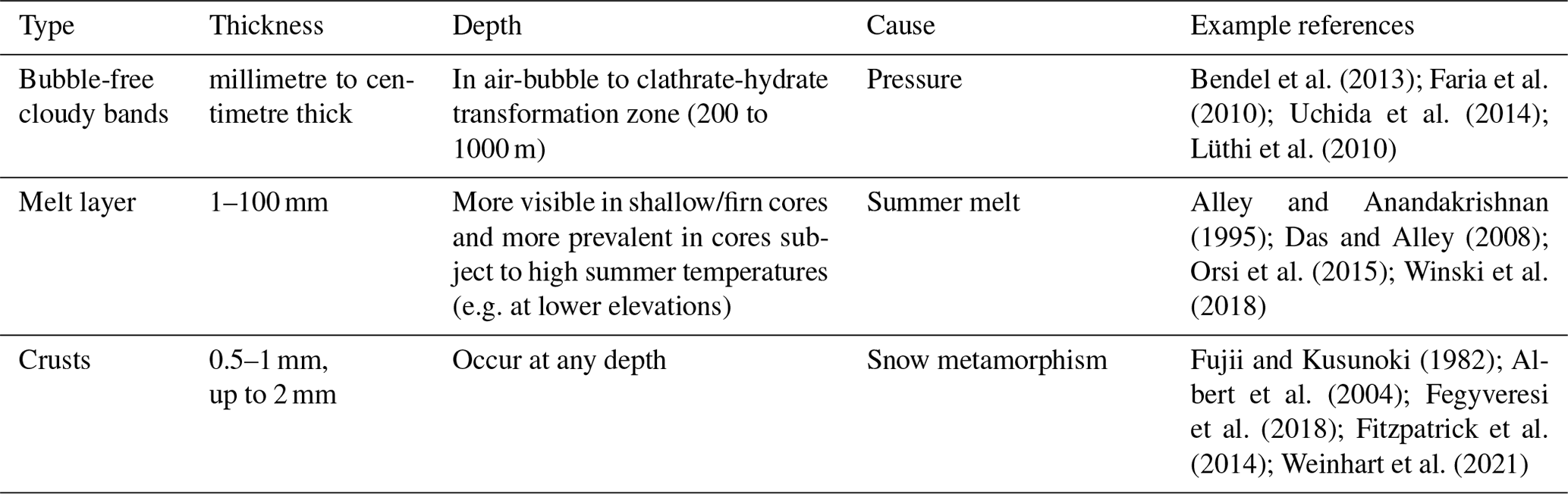

Table 1 Description of three types of bubble-free layers.

Law Dome is an ice cap on the coast of East Antarctica, with a climate impacted by large weather systems generated in the Southern Ocean (Bromwich, 1988; Udy et al., 2021; Jong et al., 2022). Thus, the ice at Law Dome broadly preserves climate signals of East Antarctica, as well as the Indian Ocean and southwest Pacific Ocean. The Dome Summit South (DSS) ice core site (66.77^∘ S, 112.81^∘ E; Fig. 1) is located approximately 4.7 km south-southwest of the Law Dome summit at an elevation of 1377 m (Roberts et al., 2017; van Ommen and Morgan, 1997). The DSS ice core site is a dry snow zone with a low mean surface temperature (−21.8 ^∘C), relatively moderate wind speeds (∼ 8.3 m s⁻¹) and a high accumulation rate of ∼ 0.680 m yr⁻¹ ice equivalent (IE) (Morgan and van Ommen, 1997; Roberts et al., 2015; Crockart et al., 2021).

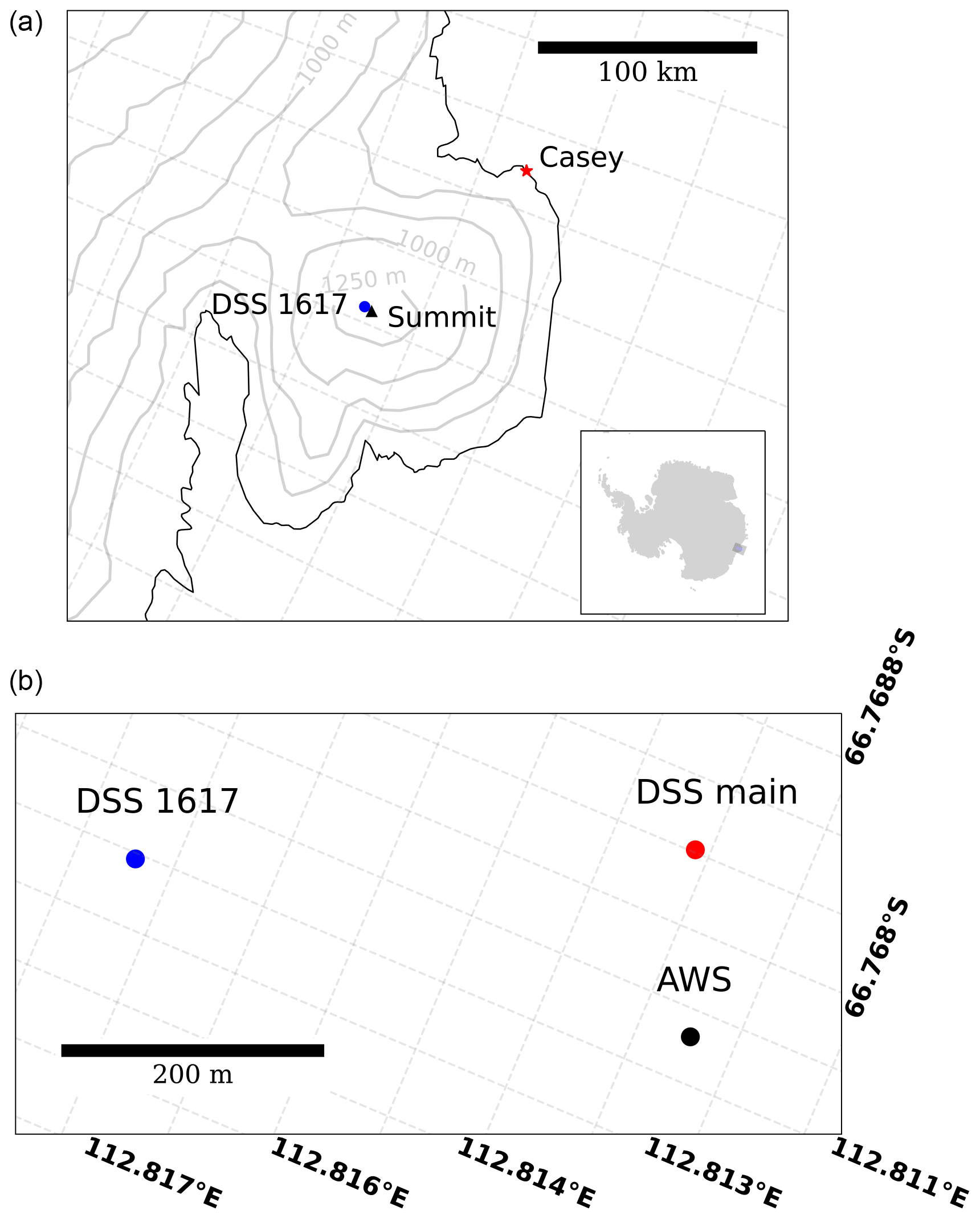
Figure 1 The location of Law Dome and the Dome Summit South (DSS) ice core site (66.77^∘ S, 112.81^∘ E) in East Antarctica near Casey Station (a). Panel (b) shows the DSS site itself with the relative positions of the DSS1617 ice core in relation to the DSS main ice core and the automatic weather station which was installed between 1997 and 2003. A snow surface height sensor operated between late 1997 and 2001, inclusive.

The DSS ice core retrieved in the 2016/17 summer (DSS1617) spans most of the recent satellite era, from 1990–2017 (Table 2). DSS site cores have been used to help understand long-term climate variability in a large region, including East Antarctica and the Indian and Pacific sectors of the Southern Ocean (van Ommen and Morgan, 2010). Upon physical inspection of the DSS1617 core, BFLs were found to occur in almost all 1 m core segments. The BFLs in DSS1617 are about 1–2 mm thick and well-defined compared to the surrounding consolidated snow or firn.

There are currently limited observations and understanding of BFL formation. Only a few studies of BFLs in the Antarctic exist, and they focus on the observation of snow surface conditions during snow surface crust formation (Albert et al., 2004; Orsi et al., 2015; Fegyveresi et al., 2018), the links between BFLs and local annual accumulation, and the implications of BFL formation on the stable isotope composition of the ice (Dadic et al., 2015). However, the exact formation mechanism of BFLs and the atmospheric processes related to BFL formation are still not clear. Previous studies have generally been undertaken during summer field observations over short time periods or are short-term studies of 3–5-year-long ice core records. This means there is a current lack of the analysis of BFL formation and its relationship to atmospheric processes over time frames long enough to statistically constrain the results.

Since this is an initial study about a new physical feature in East Antarctic glacial ice, this study is both descriptive and exploratory, under the study framework proposed by Leek and Peng (2015). For the descriptive component, we present the BFL record from DSS1617, including the seasonality and annual time series of BFLs. Longer ice cores from DSS have not been routinely scanned for visual stratigraphy using an intermediate layer core scanner (ILCS), making this study the first of its kind at this site. For the exploratory component, we conduct correlation analyses of BFL occurrence with various atmospheric processes known to drive snow metamorphism, including air temperature inversion, wind scour, accumulation hiatus, high-accumulation events and large-scale atmospheric circulation. While simplistic in its approach to the exploratory component, this study aims to increase understanding about BFL formation at Law Dome by exploring possible links between BFLs and atmospheric processes.

2 Methods

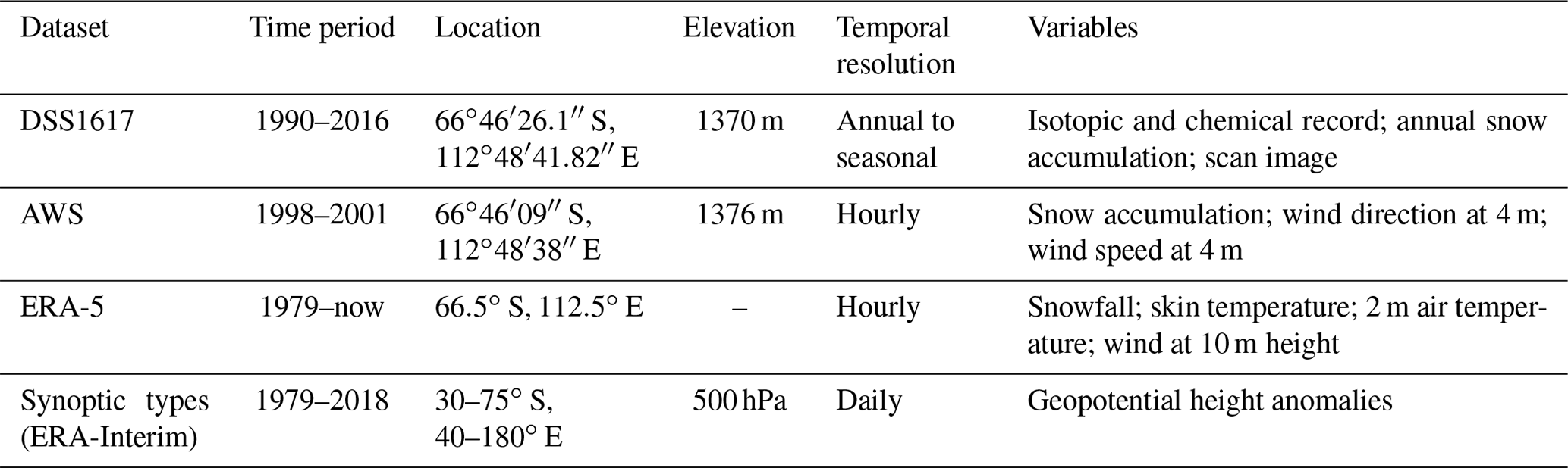
In this study, we used the recently obtained ice core record, DSS1617, which was drilled in February 2017 using an electromechanical Eclipse drill (see Table 2). The DSS1617 record is 30 m long from the surface and spans the period 1990 to 2016 (Crockart et al., 2021; Jong et al., 2022). All of the DSS1617 ice cores were scanned and analysed for trace chemistry and water-stable-isotope ratios (Sect. 2.2). In addition, we scanned the cores using an ILCS (Sect. 2.1). Climate datasets used in this study include those obtained from the atmospheric reanalysis product ERA5, data from a co-located automatic weather station (AWS) at the DSS site and a time series of daily dominant synoptic types in the southern Indian Ocean (Udy et al., 2021). More information about datasets can be found in Table 2 and in the following sections.

Table 2 Information about datasets used in this study.

2.1 Ice core scanned images

The visual stratigraphy is the most fundamental information which can be directly observed from ice cores (Svensson et al., 2005). From the ice layers, the texture, colour, micro-inclusions (e.g. dust particles, salt and other particles), and estimates of size and density of bubbles can be deduced (Alley et al., 1997; Svensson et al., 2005; Weikusat et al., 2017). Researchers can date ice cores by counting visible layers in some cases (primarily Greenlandic cores) and can identify regional-to-global climate events (e.g. summer melt, volcanic ash layers). In the majority of previous studies, the ice core visual stratigraphy profiles are recorded by drawings or photographs with limited dynamical range and poor resolution. In recent years, intermediate layer core scanning (ILCS) has been developed, with instruments specific to the scanning of whole ice cores developed by Schäfter + Kirchhoff (Germany). These ILCS instruments are designed for the visualisation of the laminar structure along the ice core by producing high-quality visual stratigraphic images (Krischke et al., 2015). Weikusat et al. (2017) used an ILCS to scan a 2774 m long ice core drilled at Kohnen Station, Antarctica ($\mathrm{75}{}^{\circ }{\mathrm{00}}^{\prime }$ S, $\mathrm{00}{}^{\circ }{\mathrm{04}}^{\prime }$ E). Krischke et al. (2015) also used an ILCS to scan polar ice cores from the Antarctic Ice Sheet (European Project for Ice Coring in Antarctica, EPICA) and Greenland (North Greenland Eemian Ice Drilling project, NEEM), and they used the stratigraphic scans to identify global climatic events, identify climate-induced precipitation and accumulation variations, and date ice cores through counting of annual visible layers where possible. In this study, we use high-resolution scans of the DSS1617 ice cores using an ILCS to identify BFLs.

The physical features of the DSS1617 ice cores were imaged by the ILCS (e.g. the DSS1617 ice core image shown in Fig. 2). The ILCS is designed to perform a transect scan of a planar ice core, providing an intermediate layer scan of the ice core for subsequent image analysis. Typically, the ice sample is cut as an ice slab, which is about 1 m long, 100 mm wide and 40 mm thick. For the data described in this study, we scanned the remaining archive half of ice cores previously sectioned for other trace chemical and isotopic analyses. The ice core surface to be imaged was planed using a mechanical thicknesser or planer, with additional polishing by hand using a stainless-steel microtome blade when necessary. The polished slab was then carefully transferred to the ILCS core carriage, which was then transferred to the ILCS base frame. The ice core slab was imaged a number of times using a range of light and depth settings to ensure good image quality regardless of ice core depth or transparency. DSS1617 was scanned as part of a larger campaign to image multiple ice core archives from East Antarctica via an ILCS instrument on loan from the Canadian Ice Core Lab to the Institute for Marine and Antarctic Sciences (IMAS) in Hobart, Tasmania. Full methods of the scanning protocols developed for this IMAS campaign are under preparation for publication elsewhere (Vance et al., 2023a).

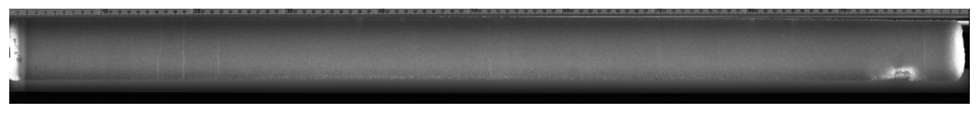
Figure 2 An example ice core scan of the DSS1617_24 ice core. The top of the core is at the left of the image, and the core is approximately 105 cm long. A ruler can be faintly discerned at the top of the image. Faint vertical white BFLs of about 1 mm thick can be discerned, located at 16.5, 19, 22.6, 52 and 99.1 cm.

The images produced by the ILCS have a cross-core resolution of approximately 13.6 pixels mm⁻¹, and a along-core resolution of approximately 19.8 pixels mm⁻¹. This resolution is sufficient to resolve the BFLs encountered in this study (width 1 to 2 mm). The transmitted light under the ice sample moves synchronously with a camera above the ice, along the core axis (Fig. 3). As the light is focused in the ice slab at a 45^∘ angle relative to the ice surface, the line scan camera can only capture light when the light is scattered into the camera by impurities or bubbles. Because light passes through transparent ice, in deep ice cores below bubble close-off with reduced scattering, BFLs are recorded as dark lines in the ice core scanned image. However, in order to scan firn cores such as those used in this study, much higher brightness settings were required to obtain adequate images. As a result, the brightness in the scanned image also increases such that clear ice in the firn cores (the BFLs) appear as white rather than dark lines. In this study, we compared the white BFLs in the ILCS images with visual inspection of the ice cores themselves under normal laboratory lighting to confirm that what we interpreted as BFLs were indeed narrow bands of bubble-free ice. In the deep core, the high isostatic pressure will compress the BFLs, forming a denser bubble-free ice layer with smoother boundaries. Due to limited isostatic pressure near the surface of the ice sheet, the boundary of the DSS1617 BFLs may not be as smooth as BFLs observed in deep ice. This may also contribute to the white appearance of BFLs in shallow ice cores, as the rough edges increase light scattering.

All BFLs were identified from visual inspection of the high-resolution images produced using the ILCS. Core drilling log books, laboratory processing log books and logbooks kept during the scanning process were consulted to help distinguish BFLs and core breaks that occasionally occurred during processing, as well as to double-check the presence and depth of BFLs, as many of the BFLs were observed and recorded during core processing. The location of each BFL relative to the depth of each core section was recorded as a dataset of DSS1617 BFL depths for subsequent analysis. This depth dataset was then mapped to year or occurrence using the DSS depth-by-age scale detailed in Jong et al. (2022).

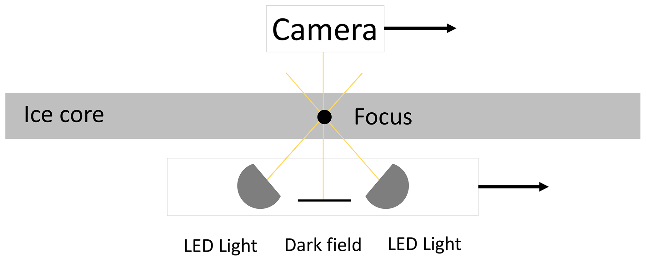
Figure 3 Ice core scanner process schematic. The arrows indicate the direction of travel of the camera and light source along the plane of the core from the top of the core to the bottom of the core.

2.2 Ice core chemical and isotopic records

The DSS1617 ice cores were sampled at 50 mm resolution for isotope and chemistry analysis, allowing for seasonal to annual dating at DSS. Water-stable-isotope records (δ¹⁸O and δD) were measured on melted ice samples using a cavity ring-down spectrometer (Picarro L2130-i), following established methods (Curran and Palmer, 2001; Palmer et al., 2001; Curran et al., 2003; Plummer et al., 2012; Jong et al., 2022). Analysis of trace ion chemistry was conducted by ion chromatography (Thermo-Fisher/Dionex ICS3000), which provides the concentrations of ions, including chloride (Cl⁻), sodium (Na⁺), magnesium (Mg²⁺), calcium (Ca²⁺), potassium (K⁺), sulfate (SO${}_{\mathrm{4}}^{\mathrm{2}-}$), non-sea-salt sulfate (nssSO${}_{\mathrm{4}}^{\mathrm{2}-}$), nitrate (NO₃) and methane sulfonic acid (MSA⁻). Analytical methods were mostly based on Plummer et al. (2012), except for a change in the cation analytical column to an Ionpac CS19 to improve detection and peak resolution of Mg²⁺ and Ca²⁺ (Jong et al., 2022).

2.3 Ice core dating

The DSS1617 ice core was dated using annual layer counting. The calendar year boundaries in the ice core (Fig. 5) were defined according to the seasonal variation in a suite of chemical and isotopic species, with the stable-water-isotope record as the primary seasonal indicator (Morgan and van Ommen, 1997; Jong et al., 2022). The summer can be indicated by the peak of hydrogen peroxide (H₂O₂), nssSO${}_{\mathrm{4}}^{\mathrm{2}-}$, MSA and the sulfate $/$ chloride (SO${}_{\mathrm{4}}^{\mathrm{2}-}$ $/$ Cl⁻) ratio, while the sea salt species (Cl⁻, Na+, Mg⁺) show peaks in winter. In addition, a volcanic reference horizon is present in the DSS1617 core, identified by an increase in sulfate signal beyond background levels (nssSO${}_{\mathrm{4}}^{\mathrm{2}-}$ peaks) related to the volcanic eruption of Pinatubo, Philippines, in 1991 (Plummer et al., 2012).

In this study, monthly dating was also undertaken on the DSS1617 ice core. Recent advances in analytical technologies have enabled ice core researchers to analyse polar ice cores at a high temporal resolution on annual to seasonal timescales (Steig et al., 2005; Iizuka et al., 2006; Hoshina et al., 2016). Fegyveresi et al. (2018) tried to determine the monthly boundaries in an ice core by equally dividing accumulation between annual boundaries into 12 parts. However, precipitation in East Antarctica can be episodic and seasonally biased (Crockart et al., 2021). Thus, monthly boundaries produced by dividing an ice core annual layer into 12 equal parts may not be accurate enough for very high resolution studies such as this one. A more accurate dating method is required to enable the detailed investigation of BFL formation, preservation and atmospheric drivers for this study. In recent years, atmospheric reanalysis data have been widely used for various studies such as surface climate characteristics of the Antarctic region as well as large-scale atmospheric forcing mechanisms modifying the surface climate variables (Hines et al., 2000; Maksym and Markus, 2008; Lenaerts et al., 2012; Costi et al., 2018). ERA5 is the fifth-generation atmospheric reanalysis product of the global climate produced by the Copernicus Climate Change Service (C3S) at ECMWF (Hersbach et al., 2019). According to the evaluation of near-surface atmospheric variables in the reanalysis products over Antarctica, ERA5 performs better than previous reanalysis products on most of the variables used here, especially temperature and snowfall (Dutra et al., 2010; Berrisford et al., 2011; Tastula et al., 2013; Albergel et al., 2018; Hoffmann et al., 2019; Gossart et al., 2019; Hersbach et al., 2020). We test the ability of ERA5 to represent local precipitation variability at the DSS1617 ice core site by comparing (1) the ice-core-derived and ERA5-derived annual accumulation between 1990–2016 and (2) the AWS snow surface height and ERA5 cumulative precipitation between 1998–2001. The significant correlation (r=0.907, p=0.01) between the ice-core-derived and ERA5-derived annual accumulation supports our use of ERA5 in ice core annual dating. The comparison between AWS snow surface height and ERA5 cumulative precipitation shows that ERA5 can reproduce snow surface increases well compared to the AWS snow surface height sensor (Fig. 4), providing confidence that ERA5 can be used for monthly ice core dating.

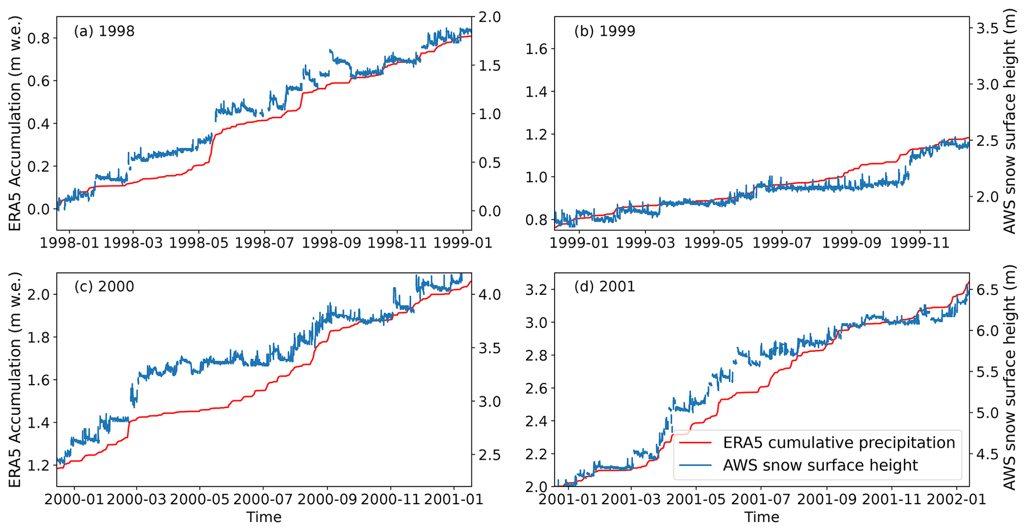
Figure 4 Comparison between ERA5 cumulative precipitation (red, metres water equivalent, left-hand axes) and AWS snow surface height (blue, metres, right-hand axes) from 1998–2001 (a, b, c, d). The correlation between ERA5 and the AWS snow surface height by month for the 48-month period is statistically significant (r=0.552, p<0.01). It is clear that ERA5 can represent the relative changes in snow surface well, with most of the rapid increases in surface height in the AWS data represented in the ERA 5 data. Note that the left-hand y axis represents the cumulative accumulation for each year shown in ERA 5 data, while the right-hand y axes show the cumulative snow surface height for each year from the AWS sensor.

Figure 5 Schematic describing the estimation of a monthly dating scale for DSS1617 to facilitate the high-resolution dating of observed BFLs. The blue lines are the annual year horizons for DSS1617 from Jong et al. (2022) (determined by using the established understanding of seasonal variation of chemistry species at DSS). The red lines are the monthly boundaries (with months numbered 1 to 12, derived using ERA5 to apportion the annual accumulation into 12 months). Thus, the annual boundary of 1998 is also the beginning of January 1998. The first red line to the left of the 1998 blue line is the boundary between month 1 and month 2 (i.e. the end of January 1998 and beginning of February 1998). The yellow lines indicate the accumulation calculated for 3 months – January, May and August 1998 – which clearly demonstrate the episodic nature of monthly snowfall in any given year.

We calculated ERA5-derived monthly accumulation by summing of ERA5 hourly snowfall within each month from 1990 to 2016. To convert ERA5-derived monthly accumulation into ice core monthly accumulation in any given year, we calculated the ratio of ice-core-derived and ERA5-derived annual accumulation. This ratio accounts for densification of ice down the core. Through this ratio for each given year, we converted the ERA5-derived accumulation for the 12 months of any given year into the proportional monthly accumulation received at the ice core site:

$$\begin{array}{}\text{(1)}& {\mathrm{Acc}}_{\mathrm{ic}}={\mathrm{Acc}}_{\mathrm{ERA}\mathrm{5}}\cdot r,\end{array}$$

where Acc_ic is the accumulation for each month in the ice core, Acc_ERA5 is the accumulation for each month calculated by ERA5 data (Table 1), and r is the ratio of ice-core-derived and ERA5-derived annual accumulation for each year. Then, based on the estimated monthly dates transposed to the ice core accumulation series, approximate depths aligned to the commencement of each month were produced by adding up the scaled monthly accumulation amounts sequentially from the beginning of each year (Fig. 5). We have high confidence in the annual (summer) layer dating in the DSS1617 ice core data (Jong et al., 2022), due to clear chemical and isotopic signatures. However, we have less confidence in being able to define within-year dates using chemistry or isotopes (especially at the monthly scale); thus, we have used the ERA5 accumulation scaled to Law Dome annual accumulation to date within-year depths.

2.4 Estimating ice core BFL position from accumulation data measured via a co-located automatic weather station

For a subset of the DSS1617 record, we can also map accumulation using locally acquired accumulation data. Hourly snow surface height was measured via a co-located AWS at the DSS site between 1997–2002 (Dome Summit South automatic weather station; date of installation: 20 December 1997) from the Australian Antarctic Division (AAD) network, which can be accessed by direct request to the AAD Centre (date of last access: 20 December 2021). The DSS AWS was equipped with a snow surface height sensor, which allowed for identification of individual precipitation events. The average annual accumulation for the DSS1617 core is 0.69 m (IE). This high accumulation rate together with accurate local snow surface height data allowed for the dating of BFLs at a sub-monthly scale for this short subset of the DSS1617 record. Thus, we attempt to estimate the date of BFL formation (or preservation) during this period from the AWS data.

From the annual layer horizons of the DSS1617 chemistry record as defined in Jong et al. (2022), the depths of each calendar year boundaries are available. We mapped these year horizons onto the scanned images of the DSS1617 cores using the core number and length measurements of each core. In each year, the location of every BFL is identified in the ILCS images. We calculated the distance of each BFL from the prior year horizon and then transcribed this to the fraction of the net snowfall surface height gain for that year from the AWS data by assigning 1 January to 0 % and 31 December to 100 %. For example, if a BFL was located at 25 % of the total accumulation for the year it occurred in, we determined this BFL to occur when the AWS snow surface height increased by 25 % of the total surface height increase for that year. Because the AWS data are observed snow surface height variation, they are subject to both accumulation and redistribution/erosion under the sensor. This means there is rarely a steady (if episodic) increase; rather, the surface height is dynamic, with small increases occurring alongside negative surface height changes as snow is redistributed or eroded. Thus, the time when accumulation reaches a specific fraction (such as 25 %) could occur at more than one point in time. We have therefore applied a time uncertainty (error boundary) for each BFL identified during the 1997–2002 period when snow surface height was measured locally by AWS. This error boundary defines the first and last time the surface height sensor data reach the fraction of the net snowfall surface height gain for that year before each BFL. Finally, within this time error boundary, we placed the BFL at the date where the snow surface height does not return below a clear erosion boundary, as we presume that the establishment of an erosion boundary likely indicates a crust or BFL formation rather than loose surface snow. This is our estimated BFL formation date (see Fig. 6 for an example of this).

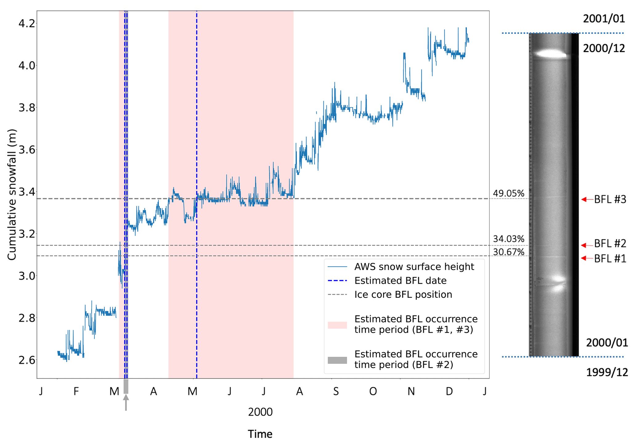
Figure 6 Aligning AWS dates of snowfall surface height changes to BFLs in the DSS1617 ice cores. ILCS imagery covering the year 2000 is shown on the right. Three BFLs were counted in the ILCS scans (red arrows). We then mapped the BFLs in the ILCS images to the calculated fraction of the cumulative snow surface height (blue line) for the year 2000 as measured by the AWS snow surface height sensor, where the fractional difference between snow surface height in 1 January and 31 December is the AWS-derived annual snow surface height change for the year 2000 (dotted grey horizontal lines at each BFL). For example, BFL #1 for the year 2000 occurred at 30.67 % of the annual accumulation (approximately March). The red and grey shading indicate the first and last time the snow surface height reached this snowfall level (to within 1 cm) to define the time period where BFL formation likely occurred (NB this period for BFL #2 is very narrow – see grey arrow on x axis).

2.5 Links to atmospheric processes

As mentioned in Sect. 1, the relationship between BFLs and climate in previous studies has mainly been detected by summertime field observations of snow surface crust formation, and there is a lack of full-season, long-term research. Here, we make an attempt to detect the relationship between atmospheric processes and DSS1617 BFLs over the past 27 years. Long-term meteorological records for 1990–2016 at the ice core sites are therefore required.

Time series of daily synoptic types from Udy et al. (2021) are used, which characterised the daily dominant synoptic types in the southern Indian Ocean for 1979–2018 by using self-organising maps. In this dataset, similar circulation patterns (500 hPa geopotential height anomalies) were grouped into nine synoptic types. During 1979–2018, each day is assigned one of the nine synoptic types. Time series of the nine synoptic types provide daily large-scale synoptic patterns over the southern Indian Ocean adjacent to the DSS site, which are then used to investigate the relationship between large-scale atmospheric circulation and DSS1617 BFLs.

In addition to large-scale atmospheric circulation, local atmospheric processes that are occurring over tens to thousands of metres at Law Dome may also be related to BFL occurrence, including surface-based temperature inversions, wind scour, accumulation hiatuses and high-precipitation events. As no dataset of these variables exists, we use climate variables from ERA5 (Table 2) from 1990–2016 to detect their date of occurrence and then produce the time series required.

We selected atmospheric process events by setting an exceedance threshold. First, we conducted a sensitivity test, choosing the threshold which resulted in the highest correlation coefficient between the number of BFLs per year (and per month) and the number of atmospheric processes per year (Fig. 7). This gave the highest possible correlation between BFL occurrences and each atmospheric process. Then, this choice of threshold was assessed to ensure physically realistic values were chosen. Unrealistic thresholds were removed, and the threshold resulting in the next-highest correlation coefficient was again assessed. This process was repeated until the threshold with a physically realistic value giving the highest correlation coefficient was found (see Table 3 for the final thresholds determined for each atmospheric process).

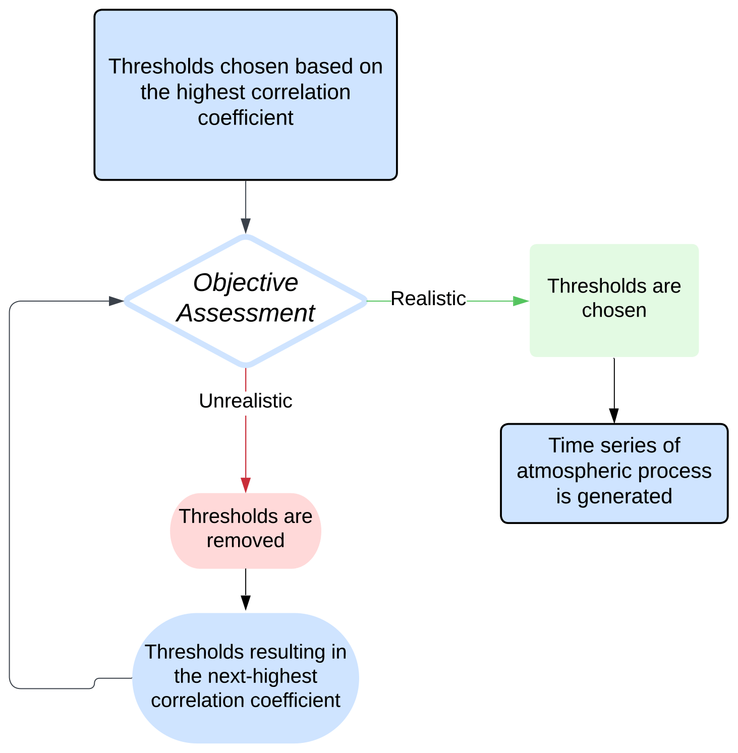
Figure 7 Sensitivity test conceptual flowchart. Thresholds of atmospheric processes were chosen based on the highest correlation coefficients detected in the initial analysis. Then, an objective assessment of whether the threshold was realistic was made, at which point the time series of the specific atmospheric process was generated or the initial step was redone using the next-highest correlation coefficient. This ensured that realistic thresholds that maximised any probable statistical relationships were investigated.

A surface-based temperature inversion is the phenomenon in which the air above the snow surface is warmer than the air temperature at the snow surface, which can lead to upward vapour transport between snow layers, which condenses at the snow surface and forms a crust. In general, a temperature inversion can be detected by measuring air temperatures at different heights. Adolph et al. (2018) suggest that the difference between skin and 2 m temperatures from satellite remote sensing has the potential to be used to detect the existence of temperature inversions. Here, we used hourly 2 m air temperature and skin temperature from ERA5, calculating the temperature difference between them to obtain inversion strength (TIS):

$$\begin{array}{}\text{(2)}& \mathrm{TIS}=T_{\mathrm{2}\mathrm{m}}-T_{\mathrm{skin}}\end{array}$$

where T_2 m is the 2 m air temperature, and T_skin is the skin temperature. Here, a temperature inversion is defined as T_2 m>T_skin, or TIS > 0. Since BFLs only occur between 0–7 times per year, we needed to develop an exceedance threshold for temperature inversions that similarly only occurs a few times per year. In this case, the two variables important for temperature inversion events are TIS and the duration (D_TI). We tested a series of thresholds for TIS (from 0 to 10 K) and D_TI (from 1 to 24 h) to filter temperature inversion events which are sufficiently strong in magnitude and duration. Based on different combinations of TIS and D_TI according to our sensitivity test framework, we produced a corresponding annual time series of exceedances and then we compared the annual total time series of temperature inversion exceedances with the annual total time series of BFLs. There are several TIS and D_TI thresholds combinations that can produce the same number of annual temperature inversion events occurrence at the same level as BFLs. Among them, the combination of thresholds based on the annual temperature inversion time series most related to BFLs was chosen as the final threshold (tis and d_TI, a temperature inversion event is identified by TIS > tis, D_TI > d_TI) (see Table 3 for final thresholds). Seasonal and annual time series are produced for correlation tests with BFLs.

An accumulation hiatus is defined as a period of time with little to no snow accumulation (Courville et al., 2007). Thus, the main variables for accumulation hiatus event detection are daily accumulation (A) and hiatus duration (D_AH). A is calculated by summation of ERA5 hourly snowfall data in each day. As with the threshold tests before, the threshold D_AH (d_ah) and threshold A (a_ah) were determined from a series of sensitivity studies (D_AH: 0 to 20 d; A: 0 to 0.6 m) to detect accumulation hiatus events that exhibited unusually low daily accumulation and long durations. Seasonal and annual time series were also produced for correlation tests with BFLs.

Daily accumulation (A) and duration (D_HP) are also important for characterising high-precipitation events. Using similar tests as for accumulation hiatuses, the threshold duration (d_hp) and threshold precipitation (a_hp) were determined to detect high-precipitation events by satisfying D_HP > d_hp and A > a_hp. Seasonal and annual time series for high-precipitation events were produced for correlation tests with BFLs.

Wind scour occurs where strong katabatic winds persistently polish the ice surface (Fisher et al., 1983). Thus, the main quantities of interest in detecting wind scour events are wind speed and wind persistence. The 10 m u-component of wind and 10 m v-component of wind in ERA5 were used to calculate the 6 h average wind speed (S) and 6 h average wind persistence (P). P is a calculated wind persistence metric (Fraser et al., 2016) defined as

$$\begin{array}{}\text{(3)}& P={\displaystyle \frac{\sqrt{U^{\mathrm{2}}+V^{\mathrm{2}}}}{S}},\end{array}$$

where U is the mean zonal wind component in 6 h, V is the mean meridional wind component in 6 h and S is the mean wind speed in 6 h. P gives a number between 0 to 1, with a value of 1 indicating a consistent wind direction. Here, we test a series of thresholds for S (0–20 m s⁻¹ in increments of 0.1) and P (0–0.9999 in increments of 0.0001). As with previous atmospheric exceedances, we select the mean wind speed thresholds (s) and wind persistence thresholds (p) that can reduce the number of exceedances to about 5 yr⁻¹ and result in the highest correlation between annual/seasonal total wind scour exceedances and BFLs. Based on this, seasonal and annual time series were generated for correlation tests with BFLs.

To explore the links between atmospheric processes and BFLs, we tested whether a statistically significant correlation between the time series exists. As mentioned previously, we produced annual time series and seasonal (3-monthly) time series for all atmospheric processes and BFLs, and then we calculated the correlation coefficients. The correlations were considered significant at a p value of ≤ 0.05.

Although we can produce monthly time series for both BFLs and atmospheric processes, we elected to only report correlations between time series at annual and seasonal timescales, due to lower confidence in monthly ice core dating. Our BFL dating method relies on snow accumulation, which records the time when the BFLs are buried by snowfall. However, BFLs may form during precipitation or at any time between two snowfall events, but they are only recorded in the ice core record by the precipitation after formation. For example, if a BFL formed in December but the formation event was followed by an accumulation hiatus of weeks (or longer), this BFL would be preserved by a snowfall event in January. In this case, the monthly time series would record it as a BFL occurrence in January rather than December the previous year. However, in using a seasonal time series, this formation versus occurrence issue is reduced, which ameliorates the formation versus preservation issue. While the DSS1617 ice core site is a high-accumulation site and accumulation hiatuses lasting months in duration are rare, for this initial study we elected to use seasonal time series to reduce the dating error caused by accumulation hiatuses.

3 Results

3.1 Annual and seasonal frequency of bubble-free layer occurrence

A total of 139 BFLs were identified in the DSS1617 ice cores during the 1990–2017 period, with a range of 0 to 9 yr⁻¹ (mean 5.15 yr⁻¹). No BFLs occurred in 2014, while they appeared most frequently in 2008 (nine BFLs; Fig. 8a). BFLs occurred year-round but were most commonly observed in austral autumn and winter, specifically April to July (Fig. 8b). The time series of annual total BFLs shows a marginally significant decreasing trend since 1990 (slope $=-\mathrm{0.127}$, BFLs yr⁻¹; 95 % confidence interval = [−0.220, −0.034]). However, the significance of this trend is likely to be largely influenced by 2014, which recorded no BFLs. The trend from 1990 to 2013 is insignificant (slope $=-\mathrm{0.0961}$, BFLs yr⁻¹; 95 % confidence interval = [−0.201, 0.009]).

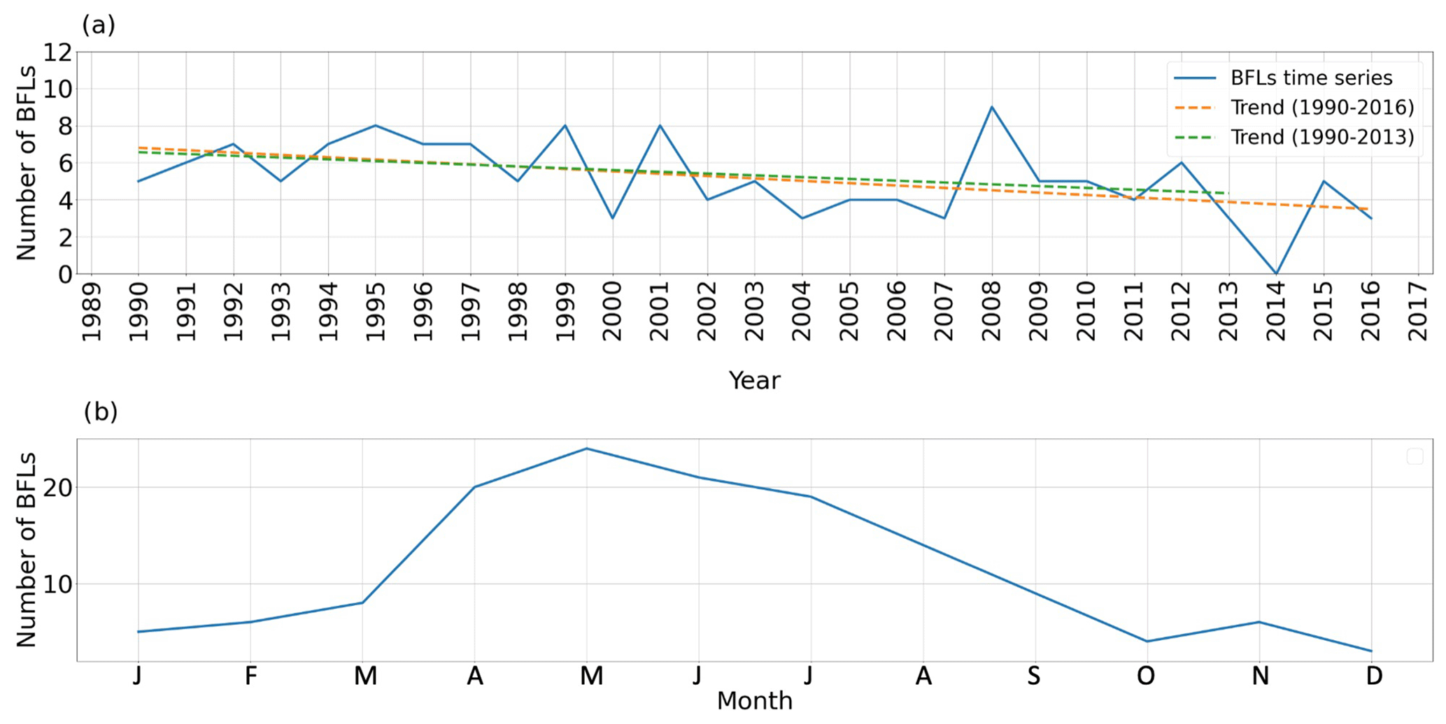
Figure 8 Number of BFLs by year (panel (a), blue), and monthly totals (panel (b), blue) in the DSS1617 ice core over the 1990–2017 period. Trends over 1990–2013 (dashed green) and 1990–2016 (dashed orange) are shown in panel (a) and discussed in the main text.

3.2 Investigation of bubble-free layer occurrence using a local automatic weather station

We investigated where BFLs occurred temporally in the ice core by comparison with the local AWS data compiled by McMorrow et al. (2004). Blue bars in Fig. 9 show the occurrence of BFLs in comparison to local snowfall accumulation measured by the AWS at Law Dome, Dome Summit South, site. It is important to note that the blue bars indicating a BFL are unlikely to denote the exact time of BFL formation in the snowpack when BFLs are preceded by a period of no snowfall for days or weeks (an accumulation hiatus). This is because BFL formation could occur at anytime during the accumulation hiatus, as the ice core record will not preserve temporal information during accumulation hiatuses.

Three BFLs occurred in 1999 that we found difficult to estimate occurrence dates for (marked by grey lines). This was because of an extended period of very low accumulation during June to December 1999. Qualitatively, most BFLs appear to occur when snow accumulates rapidly in a short period of time during high-precipitation events. This can be seen as a period where the snow surface height increases significantly over hours to days (Fig. 9). As previously noted, these high-accumulation events often occur after an accumulation hiatus. Furthermore, there are also times when this accumulation hiatus or high-precipitation event scenario is recorded by the AWS and we would expect the occurrence of a BFL, but there is no evidence in the DSS1617 core images of a BFL (e.g. March 1999 and November 2001).

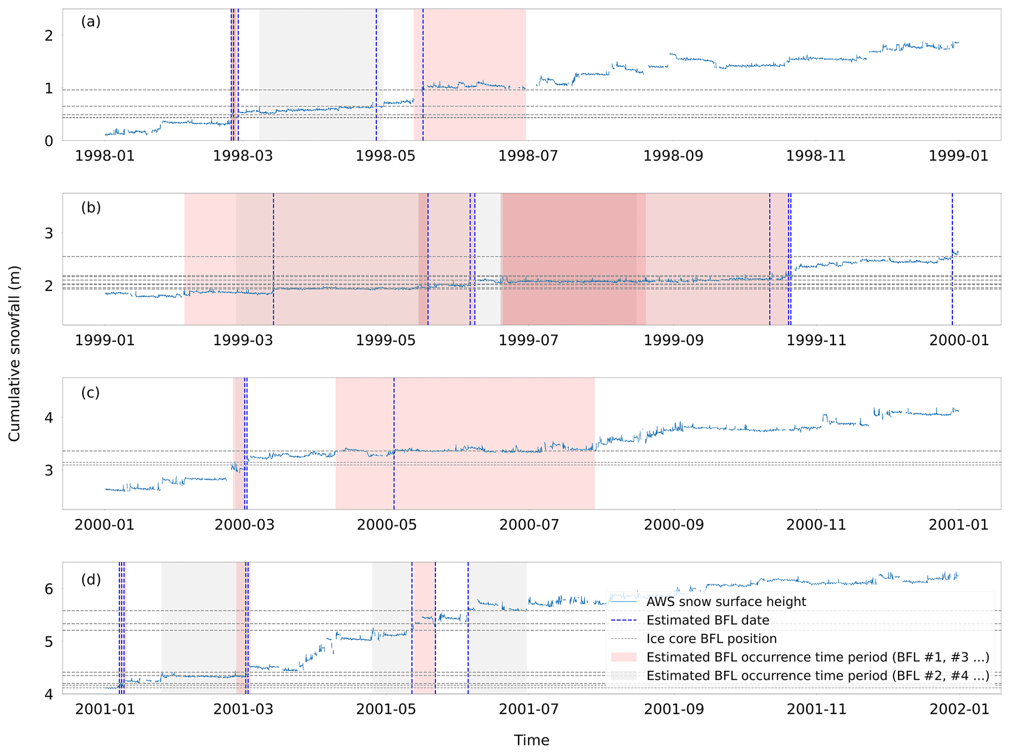
Figure 9 Cumulative snowfall and BFL occurrence during 1998 (a), 1999 (b), 2000 (c), and 2001 (d). Cumulative snowfall is shown over the time period when automatic weather station (AWS) snow surface height was detected at the Law Dome “Dome Summit South” site, approximately 500 m southeast from the DSS1617 drill site (blue time series, from McMorrow et al., 2004). Horizontal dashed grey lines indicate the fraction of total accumulation in metres water equivalent (m), where BFLs were identified in the ice cores, based on the annual layer horizons of Jong et al. (2022). Dashed blue vertical lines indicate the estimated formation date of the BFLs based on the criteria defined in Sect. 2.4. Pink and grey banding around each estimated BFL formation date indicates the qualitative boundaries for each BFL, based on the criteria in Sect. 2.4. Note different banding colours are merely to differentiate individual BFL possible formation zones, with the first BFL for each year being red, the second being grey, the third being red and so forth.

3.3 Annual and seasonal time series of atmospheric processes

We compared the time series for atmospheric processes and BFLs at both annual and seasonal scales to investigate the relationship between regional weather variability and the occurrence of BFLs. The results of comparisons of the BFLs with atmospheric processes are shown in Table 3 and Figs. 10 and 11. Accumulation hiatuses show the most significant (negative) correlation with BFLs at both seasonal and annual scales. Temperature inversions, wind scour and high-precipitation events are also significantly correlated with BFLs but only at the annual scale. However, as noted in the methods, we performed numerous correlation analyses for multiple thresholds of wind scour. Depending on the threshold, we were able to obtain marginally significant correlations at either the seasonal or annual scale, but the threshold required to achieve marginal significance needed a far greater number of wind scour events per year than the number of BFLs per year. As a result, we do not consider the wind scour results to be as robust as the results for the other three processes as we cannot discount that these may be spurious correlations related to the high number of wind scour events.

Table 3 Threshold of atmospheric processes and the corresponding correlation coefficient between BFL occurrence and each atmospheric process threshold exceedance. Values in round brackets are the thresholds/correlation coefficient values before the objective assessment and adjustment described in Fig. 7. r_a and p_a are correlation coefficients and p values between annual time series (n_a=27) of BFLs and atmospheric processes, respectively. r_s and p_s are correlation coefficients and p values between seasonal time series (n_s=107) of BFLs and atmospheric processes, respectively. Significance is assessed based on a two-tailed test at < 0.05. Bold type indicates significant correlations.

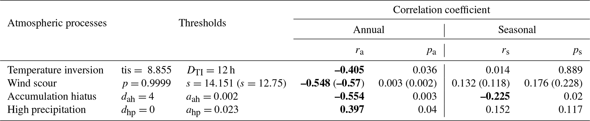
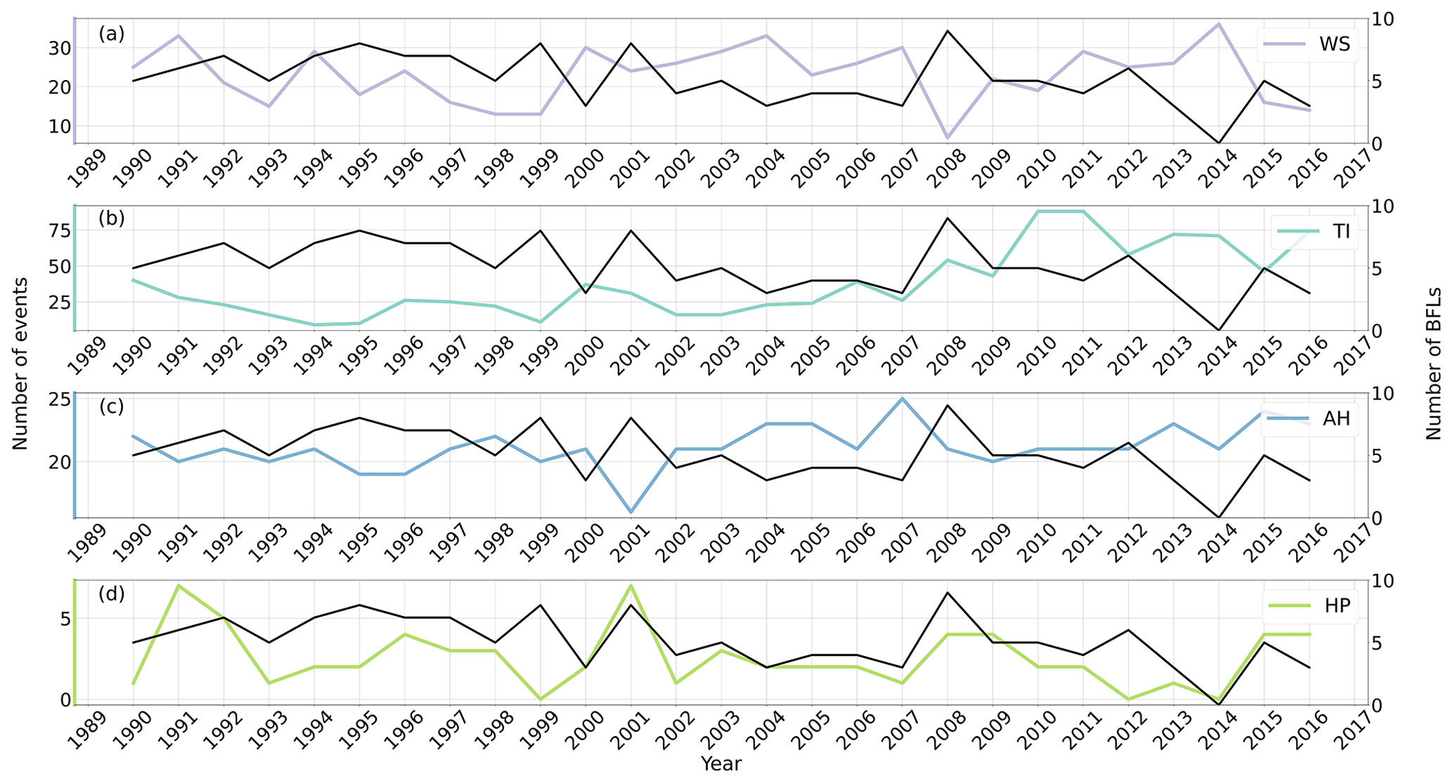
Figure 10 Time series of annual number of BFLs (black lines in all panels, right-hand axes) and atmospheric events (coloured lines, left-hand axes). The atmospheric events shown are (a) wind scour (WS) events, (b) temperature inversions (TI), (c) accumulation hiatus (AH) events and (d) high-precipitation (HP) events. See Sect. 3.3 for details on thresholds used.

Figure 11 Time series of number of BFLs (black) and number of accumulation hiatuses (AH, blue) over 1990–2016. Note that the time series is divided into the earlier period (a) and the later period (b) for visibility. Grey vertical lines denote the seasonal boundaries, with summer (DJF) and winter (JJA) shown.

3.4 Annual and seasonal time series of synoptic types

We compared the time series for synoptic types based on self-organising maps (SOMs) from Udy et al. (2021) and BFLs at both annual and seasonal scales to investigate the relationship between large-scale synoptic variability and the occurrence of BFLs. The results of comparisons of the BFLs with synoptic types are shown in Table 4 and Fig. 12. Most comparisons show an insignificant correlation with BFLs, and all are insignificant at the seasonal scale. Only synoptic types 1 and 2 (SOM1, SOM2; see Fig. 13) are significantly correlated with BFLs at the annual scale (positively for SOM1 and negatively for SOM2).

Table 4 The correlation coefficient BFLs and each synoptic type from Udy et al. (2021). r_a and p_a are the correlation coefficient and p value between annual time series of BFLs and atmospheric processes, respectively. r_s and p_s are the correlation coefficient and p value between seasonal time series of BFLs and atmospheric processes, respectively. The significance is assessed based on a two-tailed test at <0.05. Bold type indicates significant processes and correlations.

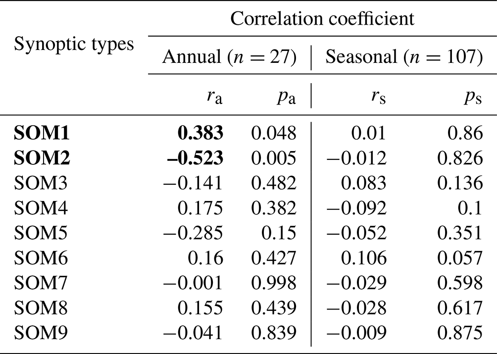
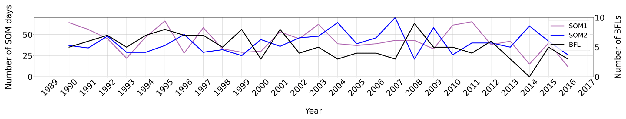
Figure 12 Time series of the annual number of BFLs (black) and annual count of the two synoptic types, SOM 1 (purple) and SOM 2 (blue), described in the study from Udy et al. (2021).

4 Discussion

4.1 Annual and seasonal frequency of bubble-free layer occurrence

The time series of annual total BFLs shows a significant decreasing trend since 1990 (slope $=-$0.127, BFLs yr⁻¹; 95 % confidence interval = [−0.220, −0.034]). However, we tested whether this significance is merely due to the lack of BFLs in 2014 (number of BFLs in 2014 is 0) by performing trend analysis over the time period 1990 to 2013. Over this time period, there is no significant trend (slope $=-$0.0961, BFLs yr⁻¹; 95 % confidence interval = [−0.201, 0.009]). Furthermore, there are two caveats that may lead to an artificially significant trend. (1) The surface firn cores may be more fragile, being composed of primarily compressed snow. Core breaks may preferentially occur at BFLs, in which case they would not necessarily be picked up by our visual counting. (2) It is possible that in very near surface firn cores, where the refraction in the imaging process is very high, we may not detect by our visual analysis faint or very thin BFLs. As a result, this trend may be spurious, and we will need to analyse longer datasets with deeper cores in the future to determine if there are longer-term trends in BFL formation.

The seasonality of BFLs indicates that at the Law Dome site the majority of BFLs occur in autumn and winter. This contrasts to the findings of Fegyveresi et al. (2018) and Weinhart et al. (2021) working at the WAIS Divide and Greenland ice core sites, respectively, where BFLs predominantly occurred in summer (WAIS) or late summer and autumn (Greenland). This seasonality suggests that BFLs may be related to seasonal climate variability rather than localised surface processes. This is important, because it indicates that DSS1617 BFLs have the potential to provide past climate information. Thus, exploring what causes BFLs has important implications for studying the climate of the Law Dome region. Secondly, the autumn/winter seasonality at the DSS Law Dome site is strong evidence that these BFLs are not melt layers. As mentioned in Sect. 1, melt layers usually form in summer due to both radiation- and temperature-related melting processes, and they often have a different appearance, being broader and with ragged edges (Das and Alley, 2005; Orsi et al., 2015). The BFLs in this study are narrow and have clearly defined edges, similar to those identified at a glazed site (80.78^∘ S, 124.5^∘ E) at East Antarctica and shown to not be due to melt processes (Albert et al., 2004). Lastly, the Law Dome site is also at an elevation and location that is unlikely to experience regular melt events even at the height of summer (van Ommen and Morgan, 1997; Morgan and van Ommen, 1997), a finding which is supported by remote sensing-based studies of melt distribution (Trusel et al., 2012).

However, there are aspects to both the previous studies and our own work that mean interpretations of the seasonality of BFLs are not yet sufficiently advanced to definitively date BFLs, either at Law Dome or other sites. Neither our dating method nor that of previous authors can currently date these features to the required accuracy (month). Fegyveresi et al. (2018) assume that the annual horizon occurs on 1 January. They then divide the annual snow accumulation into 12 equal parts to derive estimated monthly accumulation, assuming uniform accumulation rates throughout the year. Given our findings around accumulation hiatuses, high-precipitation events and highly variable monthly accumulation rates, this assumption may not hold at our site (and may be an over-simplification at the WAIS Divide site). This is an important assumption in prior studies that may need to be revisited. Weinhart et al. (2021) use five clear seasonal cycles in ${\mathrm{Cl}}^{\mathrm{-}}/{\mathrm{Na}}^{+}$ and ${\mathrm{NH}}_{\mathrm{4}}^{+}$ in the East Greenland Ice-Core Project (EGRIP, W10) to estimate summertime intervals. In this study, we use ERA5 snowfall data, combined with DSS1617 annual dating from ice core dating (which incorporates understanding of chemistry seasonal cycles at Law Dome), to calculate the monthly accumulation portion at the DSS1617 site (see Appendix A1). The DSS1617 annual dating is considered highly robust (Plummer et al., 2012; Jong et al., 2022). While using reanalysis snowfall to simulate accumulation at the ice core site will still result in dating errors, this approach is likely a more robust approach for studying BFL formation. However, given the above caveats, we analyse BFLs on a seasonal scale rather than a monthly scale in this paper. This coarsening of timescale should reduce any inherent bias resulting from dating errors compared to monthly dating.

In addition, the difference between the monthly dating approach of this and previous studies could lead to a difference in reported BFL seasonality to some extent, but these should be minor. Most DSS1617 BFLs occur during late autumn and winter, a time period with few BFLs in ice cores analysed in previous studies (Fegyveresi et al., 2018; Weinhart et al., 2021). Thus, the DSS1617 BFLs may be caused by different processes than those mentioned in previous studies.

4.2 Investigation of BFL occurrence in conjunction with local site AWS snow accumulation data

From AWS records, snow surface height at Law Dome does not increase continuously and uniformly (McMorrow et al., 2001, 2004). Not only do accumulation hiatuses and high-precipitation events occur relatively frequently, but the snow surface height also often decreases, likely driven by wind removal and erosion (Figs. 6, 9). Here, we note in several instances that the snow surface height erodes to a certain level of apparent resistance. This resistance level constitutes a dynamic barrier, which arrests further erosion. For example, in the AWS accumulation record after the fifth BFL in 1998 (Fig. 9a) and the third BFL in 2000 (Figs. 6, 9c), the snow surface height becomes eroded back to the same accumulation boundary. From these facts, we infer that such barriers could be BFLs.

The DSS1617 ice core preserves an extremely low accumulation year – 1999 – that is unusual both during the satellite era and over recent centuries (Fig. 9 and van Ommen and Morgan, 2010). Without sufficient accumulation, seasonal BFL dating in 1999 becomes challenging. Compared with numbers of BFLs in other years, there is a lower-than-average number of BFLs in 1999; however, their appearance is qualitatively different to other years in that they are crooked, broken and/or not perpendicular to the plane of the core. This may be related to the extremely low annual accumulation in this year (van Ommen and Morgan, 2010). If BFLs in years of extremely low accumulation are unlikely to present as a straight line shape, this may be evidence that sufficient snowfall plays an important role in BFL preservation. If so, while low accumulation years may lead to BFL formation, sufficient accumulation is needed to preserve them in the ice core record. In order to disentangle formation and preservation of BFLs, as well as the relationship between episodic accumulation (i.e. event scale hiatuses and precipitation) and annual accumulation (yearly total), we will need to investigate other ice core records over the satellite era and also over longer timescales.

4.3 Annual and seasonal time series of atmospheric processes

From Table 3, the number of accumulation hiatuses per year is the only atmospheric process which is significantly correlated with DSS1617 BFL occurrence on both annual and seasonal timescales ($r_{\mathrm{a}}=-\mathrm{0}$.554, p_a=0.003; $r_{\mathrm{s}}=-\mathrm{0}$.225, p_s=0.02). This is strong evidence that accumulation hiatus events are related to the formation of BFLs. This negative correlation indicates that years with more short-term accumulation hiatuses result in fewer BFLs in the DSS1617 ice core. From the AWS records in Sect. 4.2, we also know that accumulation hiatuses occur frequently at the DSS ice core site (McMorrow et al., 2004). As mentioned in the introduction, this study aims to increase understanding about BFL formation at Law Dome by exploring possible links between BFLs and atmospheric processes. The significant relationship between BFLs and the number of accumulation hiatuses provides direction for future research. In future studies, we plan to concentrate on any links between accumulation hiatuses and BFLs by exploring BFL formation mechanism(s) and the role of accumulation hiatuses using snow-pack models.

From Table 3, the number of temperature inversions, high-precipitation events and wind scours per year only show a significant correlation with BFLs at the annual scale, not seasonally. This may suggest more complex relationships with BFL formation than accumulation hiatuses. The four atmospheric processes considered exhibit considerable interplay and inter-dependence. We selected atmospheric process events by setting an exceedance threshold, which means the results are highly dependent on the values of each threshold and the duration of each event. As a result of this complexity, accurately detecting relationships using single-variable correlations is difficult as the influence of multiple atmospheric processes on BFLs cannot be effectively explored. An example of this complexity is the possibility that precipitation may be needed to preserve the BFLs after formation. In addition, previous studies (Fujii and Kusunoki, 1982; Albert et al., 2004; Fitzpatrick et al., 2014; Fegyveresi et al., 2018; Weinhart et al., 2021) suggest that these processes acting in combination may be important drivers of BFL formation. On this basis, temperature inversion, high precipitation and wind scour should still be considered in future studies as the combined effects of these three atmospheric processes may influence BFL formation.

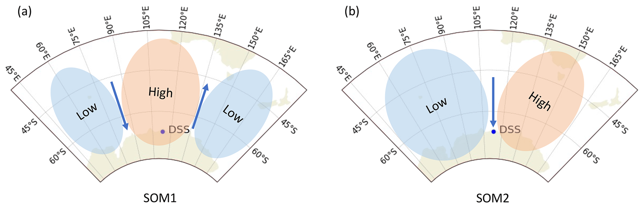
Figure 13 Schematic representation of self-organising maps (SOMs) 1 (a) and 2 (b) from Udy et al. (2021). The extent of the 500 hPa geopotential height pressure anomalies are representative of those in Udy et al. (2021). Arrows represent the direction of circulation, and the position of the Law Dome, Dome Summit South, site is shown.

Future work will utilise the SNOWPACK model (Bartelt and Lehning, 2002) to further analyse the formation mechanism of BFLs. SNOWPACK is a vertical, one-dimensional multilayer land-surface snow model, with up to several hundred layers. Based on previous crust studies and the research presented here, we believe that BFLs could form within the upper millimetre to centimetre of the snow surface. The large number of model layers allows for accurate simulations at the small surface depths we will target. Based on meteorological data, SNOWPACK can simulate the development of the snowpack and produce snow profiles. As well as the primary state variables which are common in general snow models (temperature, density, etc), SNOWPACK can also describe snow grain characteristics using four microstructure parameters, including dendricity, sphericity, grain size and bond size. Because BFLs are characterised as ice layers without bubbles, their density should be higher than the surrounding snow layers above and below them. Meanwhile, the snow grain characteristics near where the BFLs are formed should also be different from surrounding snow. Thus, the snow density and snow grain characteristics in SNOWPACK-generated snow profiles would be used to identify simulated BFLs. This approach can give us a more accurate time of BFL formation so that we can study the surrounding environmental changes and possible atmospheric processes occurring during BFL formation.

4.4 Annual and seasonal time series of synoptic types

From Table 4, BFL occurrence per year is significantly correlated with the total number of days per year where SOM1 and SOM2 are the dominant synoptic types, suggesting the BFL record may be related to large-scale atmospheric circulation to some degree. SOM1 represents a synoptic pattern where a strong positive geopotential height anomaly is located at ∼ 55^∘ S, 115^∘ E (to the north of Law Dome), with two negative height anomalies located to the east and west (Pohl et al., 2021; Udy et al., 2021). SOM2 shows a negative geopotential height anomaly at ∼ 55^∘ S, 90^∘ E (to the northwest of Law Dome), with one positive height anomaly located to the east (Udy et al., 2021) (see schematic representation of these synoptic types in Fig. 13). The cyclones over the southern Indian and southwest Pacific oceans are the main controlling factors of precipitation variation and extreme precipitation events for coastal East Antarctic regions like Law Dome (Uotila et al., 2011; Catto et al., 2015; Udy et al., 2022). During days with SOM1, the positive geopotential height anomaly blocks the passage of moist maritime air to Law Dome, leading to lower-than-average daily precipitation. In contrast, when a SOM2 pattern predominates with the positive geopotential height anomaly located further east, moist maritime air masses from the midlatitudes are channelled southward along the eastern boundary of the negative geopotential height anomaly to the East Antarctic coastline and plateau regions, which favours increased snowfall at Law Dome (Udy et al., 2022). This pattern of higher and lower-than-average daily precipitation values is likely related to the contrasting relationships we have found with accumulation hiatuses and high-precipitation events. While we are unable at this stage to disentangle the two processes, what does appear to be clear is that BFLs at Law Dome are related to meridional water vapour transport in the southern Indian Ocean and appear to record related precipitation events in the Law Dome region.

As the SOM1 and SOM2 anomalies have been defined over a large region of the southern Indian Ocean south of the subtropics (Udy et al., 2021, 2022), the correlations between BFLs and synoptic types not only indicate that BFLs have the potential to preserve large-scale atmospheric circulation, but also may be relevant to climate variability in the SW Pacific and Australia. In previous studies, van Ommen and Morgan (2010) found a significant inverse correlation between the annual precipitation from the Law Dome ice core and observed annual precipitation in southwest Western Australia. In other studies, summertime sea salt aerosol concentrations and annual accumulation in the Law Dome ice core reflected annual rainfall variability in eastern Australia and Pacific decadal variability (Vance et al., 2013, 2022). The synoptic-scale mechanism supporting this relationship has recently been defined (Udy et al., 2022), reinforcing the utility of the Law Dome record for lower-latitude climate risk analyses (see Tozer et al., 2018; Armstrong et al., 2020; Kiem et al., 2020). While these studies demonstrate the connection between the Law Dome ice core record and Australian climate, they focus primarily on annual or seasonal variability in accumulation and trace aerosol concentrations. In contrast, BFLs may be a proxy for single precipitation-related events.

5 Conclusions

This study examined bubble-free layers (BFLs) in the Law Dome DSS1617 ice core, exploring their link to weather and large-scale atmospheric patterns. BFLs are thin ice layers devoid of bubbles, distinct from previously studied phenomena. Our findings indicate that they likely form as a crust on or near the snow surface. The DSS1617 BFLs mostly appear in autumn and winter, hinting at a climate-driven formation and potential as a climate proxy. Unlike other Antarctic ice cores where BFLs peak in summer, the DSS1617 BFLs might have unique formation or preservation mechanisms. BFLs often coincide with accumulation hiatuses of 2 or more days and are linked to atmospheric patterns in the southern Indian Ocean, particularly moisture-modulating midlatitude meridional patterns. Thus, BFLs could provide insights into past atmospheric circulation changes in the region.

In future research, we will use layer-resolving snow pack models to further investigate the formation and preservation mechanism of BFLs, so as to better understand the mechanisms leading to their occurrence in ice cores. These modelling analyses will help bolster the use and development of BFLs as a new proxy record in the Law Dome ice core, as well as more broadly. We will also compare BFLs from other ice core records where available to study any commonalities or differences in formation and preservation. If the mechanism behind BFL formation can be determined (e.g. through modelling and analysis of longer records from different ice core sites), this may enable the development of a new proxy linking synoptic-scale weather events to climate variability in ice core records.