the Creative Commons Attribution 4.0 License.
the Creative Commons Attribution 4.0 License.
 | 29 Nov 2023
Regularization and L-curves in ice sheet inverse models: a case study in the Filchner–Ronne catchment
Angelika Humbert
Thomas Kleiner
Martin Rückamp
Over the past 3 decades, inversions for ice sheet basal drag have become commonplace in glaciological modeling. Such inversions require regularization to prevent over-fitting and ensure that the structure they recover is a robust inference from the observations, confidence which is required if they are to be used to draw conclusions about processes and properties of the ice base. While L-curve analysis can be used to select the optimal regularization level, the treatment of L-curve analysis in glaciological inverse modeling has been highly variable. Building on the history of glaciological inverse modeling, we demonstrate general best practices for regularizing glaciological inverse problems, using a domain in the Filchner–Ronne catchment of Antarctica as our test bed. We show a step-by-step approach to cost function normalization and L-curve analysis. We explore the spatial and spectral characteristics of the solution as a function of regularization, and we test the sensitivity of L-curve analysis and regularization to model resolution, effective pressure, sliding nonlinearity, and the flow equation. We find that the optimal regularization level converges towards a finite non-zero limit in the continuous problem, associated with a best knowable basal drag field. Nonlinear sliding laws outperform linear sliding in our analysis, with both a lower total variance and a more sharply cornered L-curve. By contrast, geometry-based approximations for effective pressure degrade inversion performance when added to a sliding law, but an actual hydrology model may marginally improve performance in some cases. Our results with 3D inversions suggest that the additional model complexity may not be justified by the 2D nature of the surface velocity data. We conclude with recommendations for best practices in future glaciological inversions.
- Article
(12597 KB) - Full-text XML
- BibTeX
- EndNote


With four parameters I can fit an elephant, and with five I can make him wiggle his trunk.
– John von Neumann
Ever since the pioneering “tutorial” of MacAyeal (1993), inversions for ice sheet basal drag – and, less commonly, englacial rheology – have been an important part of the ice sheet modeler's toolbox. In these inversions, a numerical model of ice sheet flow is compared to observations of ice surface velocity using a cost function, and the variable to be constrained (a field of either drag or rheology) is iteratively adjusted until the cost function has dropped to an acceptable level. In the 3 decades since MacAyeal's original paper, remotely sensed observations of ice sheet surface velocity have become available for nearly the entirety of the Greenland and Antarctic ice sheets, along with many smaller ice caps and mountain glaciers (Joughin et al., 2010b; Rignot et al., 2011, 2017; Fahnestock et al., 2016), while knowledge of ice sheet geometry has improved dramatically as well (Lythe and Vaughan, 2001; Fretwell et al., 2013; Morlighem et al., 2014, 2020; Bamber et al., 2001, 2009, 2013). Concurrently, the computing power available to run these models has increased enormously. Thus, it has now become routine in glaciological modeling to use inversions to study the spatial – and, with repeat observations of surface velocity, temporal – variability of the ice sheet basal drag and to initialize transient models of the ice sheet future (Joughin et al., 2004, 2006, 2009; Morlighem et al., 2010, 2013; Gillet-Chaulet et al., 2012, 2016; Habermann et al., 2013; Sergienko and Hindmarsh, 2013; Sergienko et al., 2014; Shapero et al., 2016).
However, the question remains of just how much information can truly be gleamed from ice model inversions. Fundamentally, the trouble is that a spatially resolved inversion has an infinite number of free parameters, and in a numerical implementation of the problem, the number of free parameters is determined by the discretization used, not by anything fundamental in the problem. Furthermore, the transfer function relating variations in basal shear stress to surface velocity or slope is essentially a low-pass filter (Gudmundsson, 2003), allowing dramatically different fine-scale drag fields to produce similar velocity observations (Habermann et al., 2012), and ensuring that the inverse problem (using surface velocity to infer basal stress) is ill-posed. Ill-posed inversions require regularization to create a well-posed problem and avoid overfitting noise in the data. The most common form of regularization used in glaciological inversions is Tikhonov regularization (Tikhonov and Arsenin, 1977), which involves adding an additional term to the cost function that penalizes variability in the inversion target field, usually through a measure of gradient or curvature, and combining this regularization cost (Jreg) with the original data cost term (Jobs) to create a combined cost function (J) that is minimized by the inversion. A weighting parameter, which we write as λ, controls the relative contribution of the data and regularization terms to the overall cost function that is minimized in the inversion.
Yet this introduces a new free parameter into the problem: if λ is too high, the inversion will under-fit the data, producing very little structure even if the observations could be used to infer greater detail, while if λ is too low, the inversion will over-fit the data, producing spurious structure that is not truly required by the observations. While other methods of determining the optimal regularization level, such as Morozov's discrepancy principle, have occasionally been used in glaciological inversions (e.g., Martin and Monnier, 2014), the most common way to determine the optimal value of λ is through an L-curve analysis, in which Jobs and Jreg are plotted against one another for different values of λ, ideally showing a corner (the “L” shape) at the value of λ that best balances between the extremes of over-fitting and under-fitting (Hansen, 1992; Hansen and O'Leary, 1993). This corner can be rigorously identified by measuring the curvature of the L-curve in log–log space (Hansen and O'Leary, 1993). Even when performed correctly, L-curve analysis is not perfect (e.g., Vogel, 1996); however, the actual practice of L-curve analysis in the glaciological literature is inconsistent at best, and many modelers who chose to forgo L-curve analysis do not replace it with any other method of calibrating the correct regularization level.
In this paper, we first give a brief review of the ways in which regularization and L-curve analysis have been treated in glaciological inverse models, and then we give a tutorial on how to regularize and perform L-curve analyses for glaciological inverse problems. Using an inversion of the Filchner–Ronne catchment in Antarctica as our test bed, we demonstrate how to scale misfit components, compute L-curve curvature, and select both the optimal λ value as well as a range of acceptable λ values bracketing the corner. We explore how the spatial and spectral characteristics of the solution change as λ is varied within this acceptable range. We perform a set of experiments testing the influence of mesh resolution, effective pressure, sliding nonlinearity, and flow approximation. We generate a new independent L-curve for each change in our experimental setup. Finally, we combine our various inversion results into a single best weighted-average estimate of the basal drag within our domain. We conclude with a discussion about what this approach to glaciological inverse problems enables us to learn about basal sliding and with recommended best practices for future modelers.
The original work of MacAyeal (1993) was a pioneering addition to the toolbox of glaciological modeling at the time. However, that work included no explicit regularization at all (MacAyeal, 1993, Eq. 17), instead avoiding overfitting by parameterizing the drag coefficient as a sum of Fourier basis functions and truncating the sum at low order. Indeed, in the synthetic example used in that paper, the “true” basal drag was given by only two Fourier terms, and the inversion consisted of an optimization to recover those same two coefficients. Subsequent papers using the MacAyeal method with real velocity data instead of synthetic examples obviously included a much greater number of Fourier coefficients, but they still relied on truncation of the series to prevent over-fitting rather than including explicit regularization within the cost function (Joughin et al., 2004, 2006, 2009). The question of where exactly to truncate this series was not investigated in detail other than to note that the governing equations were not accurate below wavelengths of a few ice thicknesses.
Later, Arthern and Gudmundsson (2010) introduced the method of solving the inverse problem by simultaneously solving Neumann and Dirichlet versions of the stress balance problem (i.e., solving one forward problem where the surface is traction-free and another forward problem where the surface has a Dirichlet condition given by the observed velocity, and minimizing the difference between these two solutions). This method produced a major advance in ice sheet inversions, allowing the full Stokes (FS) equations to be inverted without the need to derive the adjoint (an equation for the gradient of the cost function with respect to the inversion target field). In addition, and unlike the models in the direct MacAyeal lineage (Joughin et al., 2004, 2006, 2009), they did not rely on a series expansion representation of the drag coefficient in their derivation, removing the need for arbitrary truncation and instead representing drag coefficient on the same numerical mesh as the rest of their problem. However, they did not put any explicit regularization in their cost function either (Arthern and Gudmundsson, 2010, Eq. 3), and, consequently, they found that their algorithm produced erroneous spatial structure when given noisy velocity data (Arthern and Gudmundsson, 2010, Fig. 3). To solve this, they settled on a “heuristic” method of implicit regularization achieved by stopping their algorithm at a small number of iterations before the erroneous spatial structure had a chance to grow. It has long been known that certain types of iterative solvers can have a regularizing effect if they are stopped early (Hansen and O'Leary, 1993), and Habermann et al. (2012) developed a similar method of implicit regularization for glaciological inversions of synthetic data. However, it is notable that when those authors later applied their methods to the inversion of real data, they employed explicit regularization (Habermann et al., 2013, Eq. 4), as did later users of the Neumann–Dirichlet approach (e.g., Shapero et al., 2016).
Indeed, it is rare to find inversions of real data and real glacier geometries performed without either explicit regularization or series truncation. However, that regularization is unfortunately not always discussed in detail, and often the effect of regularization is not explored and the choice of regularization is not justified. For instance, Morlighem et al. (2010) studied spatial patterns in basal drag under Pine Island Glacier determined from inverse models, yet they gave no details on regularization other than a single sentence (in their Sect. 2.4) confirming that it was in fact present. Thus it is difficult to evaluate whether or not conclusions drawn about the detailed structure of basal drag near the grounding line may have been influenced by the choice of regularization. In other papers, regularization is performed and explained, but L-curve analysis is not performed and the particular level of regularization is not always justified. For instance, Sergienko and Hindmarsh (2013) and Sergienko et al. (2014) explicitly showed how they regularized their inversion, and they performed sensitivity experiments with several values of λ for both real and synthetic examples. However, they explicitly chose not to present an L-curve analysis, citing the possibility of L-curve non-convergence (Vogel, 1996) as their reason.
When an L-curve analysis is performed in glaciological inversions, the presentation of the L-curve can be highly variable. Hansen and O'Leary (1993) explicitly recommended that L-curves should be presented on log–log axes and that the curvature computation used to select the corner should also be performed in log–log space. However, while glaciologists have sometimes presented L-curves on log–log axes (e.g., Morlighem et al., 2013, Fig. 1), they have also employed linear–linear axes (Shapero et al., 2016, Fig. 1; Habermann et al., 2013, Fig. 5) or even mixed log–linear axes (Gillet-Chaulet et al., 2012, Fig. 3). The variable presentation styles for different L-curves are potentially problematic, as L-curve analysis is explicitly predicated on the concept of “shape”, and many of the above authors chose their optimal λ values based on a visual assessment of corner position rather than a quantitative measure of curvature. Finally, while L-curves in the glaciological literature have usually been monotonic (Morlighem et al., 2013; Habermann et al., 2013; Shapero et al., 2016), that has not always been the case (Gillet-Chaulet et al., 2012).
We do not claim that this review of regularization and L-curve analysis in the glaciological literature is exhaustive. Our intention here was merely to illustrate the spectrum of ways in which these issues have been treated within glaciological inversions. Inversions are a vital source of boundary conditions for projections of ice sheet dynamics in a changing climate (Seroussi et al., 2019), and inversions also provide a vital window into the conditions and processes at the ice sheet bed, an environment that is difficult to observe directly. L-curve analysis is an important method for ensuring that inversions are well-calibrated between under-fitting and over-fitting the data, yet the treatment of L-curve analysis and the visual presentation of L-curves has been highly variable within the glaciological literature. Even the basic question of whether glaciological inverse problems have a convergent L-curve remains unanswered.
3.1 Experimental design
In addition to regularization, we also test the sensitivity of our results to element size, flow equation, sliding nonlinearity, and the use of effective pressure. We test the influence of regularization through L-curve analysis, and we created separate independent L-curves whenever we tested anything else in our experimental setup: for instance, when we varied element size, we created a separate L-curve for each mesh that we tested. We organized our experimental setup around a reference case using the shelfy-stream approximation (SSA) in the highest-resolution mesh with a linear Weertman sliding law. We explored the influence of regularization itself by analyzing the spatial and spectral characteristics of the reference case in detail (Sect. 4 and 5). In order to test the dependence of regularization on element size, we produced L-curves using linear Weertman inversions for a series of 10 meshes (Sect. 4.4). We tested the influence of effective pressure N by producing L-curves with Budd sliding using three candidate N fields in the highest-resolution mesh (Sect. 4.5). We tested the influence of sliding nonlinearity by producing L-curves for both the nonlinear Weertman sliding law and nonlinear Budd sliding with the highest-performing N field (Sect. 4.6). We performed experiments comparing SSA inversions with higher-order (HO) inversions by producing L-curves for HO using linear Weertman sliding in mesh nos. 4, 6, and 8, along with one additional HO L-curve in mesh no. 6 using constant rheology instead of variable rheology (Sect. 4.7). All in all, the experiments presented in this paper comprise 21 independent L-curves (10× linear Weertman SSA, 2× nonlinear Weertman SSA, 3× linear Budd SSA, 2× nonlinear Budd SSA, and 4× linear Weertman HO), each composed of 25 separate inversions, for a total of 525 individual inversions. Additionally, we did a supplemental experiment where we converted the coefficient from a linear Weertman inversion into a nonlinear sliding law, and we compared the resulting converted L-curve to the L-curve computed from inversions performed directly with the nonlinear law (Sect. B1).
3.2 Setting
We model a domain covering the catchments of West and East Antarctica that feed into the Filchner–Ronne Ice Shelf (Fig. 1). This domain has a wide variety of glaciological settings, including both slow-flowing regions and fast-flowing ice streams, mountainous subglacial topography and deep subglacial basins, topographically confined outlet glaciers and relatively unconfined glaciers, along with a large floating ice shelf containing several ice rises and rumples. We choose to use a real setting based on real data for this study rather than constructing a synthetic example for several reasons: (1) we are interested in learning about the spatial and spectral characteristics of the true basal drag (Sect. 4 and 5); (2) we are interested in evaluating how good different effective pressure fields (Sect. 4.5) and sliding exponents (Sect. 4.6) are at parameterizing reality; (3) we are interested in exploring the convergence behavior of L-curve analysis with respect to model resolution (Sect. 4.4), and this is known to depend on the roughness characteristics of the true solution (Vogel, 1996); and (4) we wish to conclude by offering recommendations for future glaciological modelers (Sect. 6), and recommendations based on simplified synthetic examples may founder when tested against the complexities that arise when applying models to real datasets. We take surface (Fig. 1a) and bed (Fig. 1b) elevations, along with ice thickness and our ocean–shelf–sheet–rock mask from BedMachine Antarctica, Version 2 (Morlighem et al., 2020; Morlighem, 2020). Ice surface velocity observations needed for our inversion (Fig. 1c) are taken from a combined Landsat 8 and TerraSAR-X product created by Neckel (2022) for Hofstede et al. (2021), merged with MEaSUREsv2 (Rignot et al., 2011, 2017). We also can use the observed velocity and geometry to compute the driving stress projected onto the flow direction (Fig. 1d) which we use to estimate potential energy dissipation (Sect. A2 and A1) and to compute our first guess of drag coefficient (Sect. 3.5).
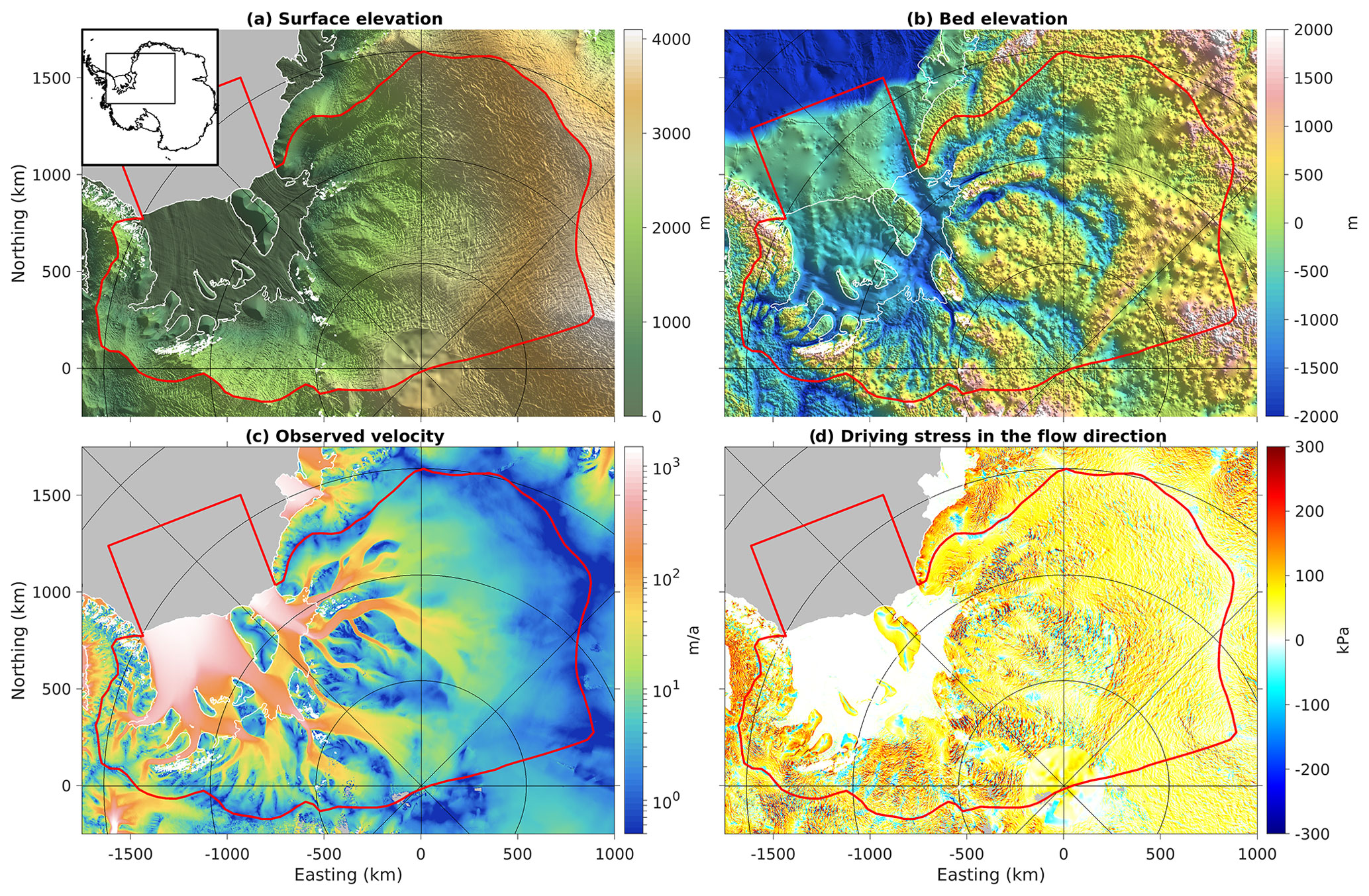
Figure 1Geographic setting of our study area. (a) Surface elevation from Morlighem (2020), with inset showing map location in Antarctica. (b) Bed elevation from the same source. (c) Surface velocity observations from Neckel (2022) and Rignot et al. (2017). (d) Driving stress in the flow direction computed from ice geometry and observed velocity vectors. Red line in all maps shows outline of model domain. The domain extends beyond the calving front to facilitate transient modeling of ice front motion, which we do not discuss in this paper. White lines show ice edge and grounding line. Graticule uses lines at 5∘ in latitude and 45∘ in longitude. Plots (a) and (b) employ hillshading to emphasize structure and texture, using two perpendicular light sources from grid north and grid east.
3.3 Ice sheet model
We use the Ice-Sheet and Sea-level System Model (ISSM; Larour et al., 2012) to simulate the catchment of the Filchner–Ronne Ice Shelf. We use the shelfy-stream approximation (SSA, also called shallow shelf approximation; MacAyeal, 1989). SSA reduces the 3D problem of ice flow to a vertically integrated 2D problem in the map-view plane, thus neglecting all but the xx, yy, and xy terms in the stress and strain-rate tensors. SSA is most valid in fast-flowing ice streams and outlet glaciers, where the ice is flowing primarily by basal sliding. The SSA equations are also self-adjoint for linear sliding laws (MacAyeal, 1993), and they were the first version of the ice sheet stress balance equations to be used in an inversion (MacAyeal, 1993). The SSA equations are
where H is ice thickness, is the vertically averaged viscosity, u is the horizontal ice velocity vector, ∇() is the gradient operator in the horizontal plane and ∇T() is its transpose, I is the identity matrix, ∇⋅() is the divergence operator in the horizontal plane, τd is the gravitational driving stress, and τb is the basal stress, which we infer indirectly using our inversion. The driving stress is computed from the ice sheet geometry by , where ρi is the density of ice, g is the acceleration due to gravity, and zs is the ice sheet surface elevation. At the inland lateral boundaries of the domain we use Dirichlet conditions given by the observed velocity. The effective viscosity is computed from the nonlinear rheology of ice (Glen, 1953) using
where is the vertically averaged rheological stiffness parameter, is the effective strain rate, and n=3 is the rheological exponent. We use the SSA equations for the majority of our experiments, but we also ran several experiments using the 3D higher-order (HO) equations (Blatter, 1995; Pattyn, 2002) to compare the effect of using a 3D model instead of a 2D one. We do not list those equations here for brevity. We compute the rheological stiffness needed for both sets of equations using a 1D thermal model, described in Sect. A1. We solve the equations for both models on spatially refined unstructured meshes described in Sect. A2. We used a multi-wavelength interpolation procedure to interpolate gridded data products onto our meshes in a way that prevented aliasing where the mesh is coarse while still preserving high-resolution spatial structure where the mesh is fine (Sect. A3).
3.4 Sliding law
For our basic model, we use a Weertman-type sliding law (Weertman, 1957):
where τb is the basal shear stress vector, C is a spatially variable drag coefficient, ub is the basal sliding velocity vector, and m is the slip exponent. For most of our experiments we used linear Weertman (m=1); however, we also ran tests with nonlinear Weertman sliding using m=3 and m=5, the results of which we present in Sect. 4.6. When testing the effect of sliding laws with effective pressure, we use a Budd-type sliding law (Budd et al., 1979):
where is the effective pressure at the ice base, and Pi and Pw are ice and water pressures, respectively. Budd sliding is not the only sliding law to incorporate N, nor is it necessarily the most advanced law to do so (e.g., Schoof, 2007; Gagliardini et al., 2007; Tsai and Gudmundsson, 2015). However, Budd sliding continues to be used in recent glaciological publications (e.g., Brondex et al., 2019; Barnes and Gudmundsson, 2022; Kazmierczak et al., 2022), and a Budd law has the advantage of being directly comparable to a Weertman law with the same stress exponent, allowing us to test the influence of N with all else held constant. We test three different sources for N:
where Nop is N assuming a perfect hydraulic connection to the ocean, and allowing negative water pressures; Nopc is N determined from ocean pressure with a strict cutoff at zb=0; and NCUAS is N taken from the hydrology model CUAS (Confined-Unconfined Aquifer System model). CUAS is an equivalent thin-layer hydrology model using confined–unconfined aquifer equations and parameterizations for efficient drainage and the opening of cavity space by ice sliding (Beyer et al., 2018; Fischler et al., 2023). We force CUAS using the melt rate estimated by the same 1D thermal model used to estimate ice rheology (Fig. A1e). We run CUAS on a 1 km regular grid and then interpolate the results onto our ISSM mesh. Nopc is a commonly used approximation in the glaciological literature, and we felt it was important to test it here. However, Nopc contains a sharp discontinuity in gradient around the zb=0 contour, so our motivation for allowing negative water pressures in Nop is to eliminate that discontinuity and test for the optimal regularization when N was a simple linear function of zb. In both approximations N is strictly positive throughout our domain.
We show a comparison of the three N fields in Fig. 2. Nop is the smoothest, as it is a simple linear function of ice thickness and bed elevation. It also has the most range, as inland regions with a very high ice surface elevation and bed elevation above zero have a large ice overburden pressure combined with a negative water pressure, producing very high N. Nopc has a broadly similar large-scale structure to Nop, but with more visible short-wavelength structure introduced by the cutoff in water pressure at zb=0. The range of Nopc is also less than the range of Nop, as the high-elevation inland regions are no longer allowed to have negative water pressure and thus have lower N. NCUAS has the lowest range of the three, with a maximum of about 10 MPa, or a factor of 3–4 less than the other two. The spatial structure of NCUAS is more complex than Nop but also appears more ice dynamically reasonable, at least under visual inspection, than Nopc. The spatial structure of NCUAS is a close visual match to the overall structure of the ice-sheet velocity field (Fig. 2c, cf. Fig. 1c), likely as a result of the fact that we used estimated shear heating to produce the melt rate forcing for CUAS (Fig. A1e).
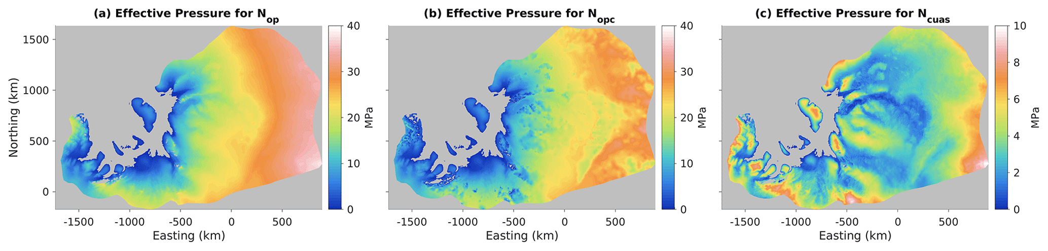
Figure 2Comparative maps of effective pressure N. (a) Nop, or N computed assuming a perfect connection to the ocean and allowing negative water pressures. (b) Nopc, as Nop but without allowing negative water pressures. (c) N computed by the hydrology model CUAS. Note change in color scale in panel (c).
3.5 Cost function
We use a single observational misfit and a single regularization term in our cost function. Our observational misfit is the L2 norm of the absolute velocity misfit:
where Jobs,raw is the raw observational component of the cost function, Ω is the map-view model domain, and are the two components of the horizontal velocity vector. Our regularization misfit is the L2 norm of the magnitude of the gradient of the friction coefficient:
where Jreg,raw is the raw regularization cost and is the internal ISSM friction coefficient. There is no mathematical or physical reason why the leading constant of the sliding law should be squared; MacAyeal (1993) squared the constant to ensure it remained positive, but this same goal can be achieved by simply setting a lower limit within the inversion code. We therefore exclusively analyze results for C, not k, when analyzing our inversions. However, we do expect C to vary by many orders of magnitude, and the regularization term may therefore under-penalize spatial structure in low-drag areas as compared to high-drag areas. Taking the square root of the drag coefficient before computing the regularization term halves the dynamic range, and thus we expect this problem to be less of an issue for k than for C.
Before combining the data and regularization cost terms, it is useful to scale them according to estimates of their characteristic magnitude. Scaling the cost function terms is valuable for two reasons: (1) it allows us to easily identify the region of parameter space that we need to search in our L-curve analysis, and (2) it ensures that the regularization parameter is both unitless and readily interpretable in terms of relative weight placed on the two component terms. Without scaling, the regularization parameter would have obscure units, it would be difficult to identify the region of parameter space near the corner of the L-curve to search for the optimal regularization, and there would be no basis for judging whether a given level of regularization was “large” or “small”.
The characteristic scale of the data term is readily given by the variance of the velocity observations themselves:
where Sobs is the characteristic scale of Jobs,raw, is the magnitude of the observed velocity vector, A is the area of the grounded domain, and σobs is the root-mean-square (rms) variability of the observed velocity magnitude.
Computing the characteristic scale of the regularization term is more complex than computing the characteristic scale of the data term, because the magnitude of the regularization term depends on the gradient of the unknown drag coefficient. We computed the characteristic scale of the regularization term based on the mean-square gradient of a reference sinusoid with a wavelength given by the mean ice thickness and an amplitude given by an estimate of the standard deviation of the drag coefficient. We estimated the standard deviation of the drag coefficient by computing a first guess based on the ratio of driving stress and observed velocity:
where kguess is the guess of k, and is the driving stress projected onto the flow direction (Fig. 1d). For Weertman sliding, we set N=1 in the above equation. For Budd sliding, we use a minimum N value of 100 Pa to prevent division by zero, and for both sliding laws we use a minimum velocity value of 10 cm a−1 for the same purpose. We then compute σk, the standard deviation of kguess, and we use it to define a reference sinusoid, . The gradient of this sinusoid is , and the mean-square amplitude of the gradient is . Plugging the mean-square amplitude of this perturbation into Eq. (9) and assuming an area of integration equal to the grounded domain yields the scale estimate:
where Sreg is that characteristic scale of the regularization term Jreg,raw.
We then use the characteristic scales to normalize both components of the cost function:
where Jobs,Jreg are the scaled dimensionless cost function terms. The final cost function is a linear combination of the two scaled terms:
where J is the total cost function that is minimized by the inversion and λ is a dimensionless Tikhonov regularization parameter (Tikhonov and Arsenin, 1977). We determine the optimal λ value through an L-curve analysis. We tested 25 logarithmically spaced samples in the range . For each sample, we run the inverse model to convergence and record Jobs and Jreg. We then used a curve-fitting procedure to fit a smooth curve to the discrete samples of Jobs and Jreg. We computed the second derivative of the smoothed curve in log–log space and used this as the basis for selecting λbest, the best fit corner value of the L-curve, along with minimum and maximum acceptable values, λmin and λmax, that bracket the range of the corner of the L-curve. We discuss the curve-fitting and λ estimation procedure in Sect. A5.
4.1 L-curves
The L-curve for our reference case of mesh no. 1 and linear Weertman sliding is shown in Fig. 3a. Our model results form a well-defined “L” shape in (ln (Jreg),ln (Jobs)) space, and the visual impression of an “L” shape can be trusted in this figure because we have taken care to scale the plot so that a decade of dynamic range takes the same amount of space on both axes. Both components of the misfit are monotonic functions of λ, and our smoothed tradeoff curve runs very close to the original model points (Fig. 3a, b), giving us confidence in our curve-fitting procedure. Previously published inversions have sometimes been vexed by problems such as deviations from L-curve monotonicity or outlier models that fall far from the smooth L-curve (e.g., Gillet-Chaulet et al., 2012, Fig. 3); while we cannot be sure of what caused these results for other authors, during development of our model setup, we found that such issues were often an indication of lower-level numerical problems such as suboptimal choice of solvers, overly lax convergence tolerances, or overly complex mask topologies. Once those issues were fixed, we found that smooth monotonic results such as those in Fig. 3 were typical for all of our inversions.
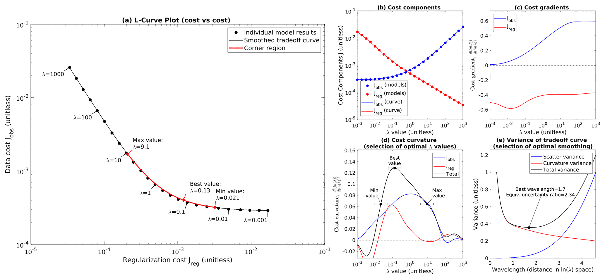
Figure 3Example L-curve for mesh no. 1. Large plot (a) shows the L-curve, a log–log plot of Jreg vs. Jobs. Black circles show individual inversions, the black line shows the smoothed tradeoff curve fitted to the individual models, and the red region highlights the corner of the L-curve. Note that we have scaled the axes in plot (a) so that 1 order of magnitude in Jreg takes up precisely as much space as 1 order of magnitude in Jobs. (b) Plot of both misfit components (Jreg and Jobs) against λ. (c) Cost gradient as a function of λ. (d) Cost curvature as a function of λ, with selection of minimum, best, and maximum λ values annotated. (e) Selection of optimal smoothing wavelength, showing scatter and curvature variance (Vs and Vc), selection of optimal smoothing wavelength, and equivalent uncertainty ratio for λ on a linear scale.
Far from the corner region, both limbs of our L-curve tend towards straight lines, but for the large-λ limb this line is sloping, indicating a power-law relationship between Jreg and Jobs, while for the small-λ limb this line is horizontal, indicating an asymptotic approach to a best achievable Jobs (Fig. 3a). The straight-line nature of the limbs can be confirmed by looking at the gradient of the cost terms: both terms approach constant gradient for large λ, while Jobs smoothly approaches zero gradient for small λ (Fig. 3c). The low-λ limb corresponds to the “flat” part of the L-curve identified by Hansen and O'Leary (1993, Sect. 4.1), while the high-λ limb corresponds to the “vertical” part, although for linear sliding the slope of this limb is far from vertical (for nonlinear sliding the slope of this limb increases, as we show in Sect. 4.6). The power-law nature of the large-λ limb may potentially explain the results found by Habermann et al. (2013). Those authors found that their L-curve lacked a corner when plotted on log–log axes, motivating them to use linear axes instead (Habermann et al., 2013, Sect. 3.4). While we cannot be certain what caused them to find this result, our own results suggest that they may have been testing λ values in the large-λ limb. Normalizing cost function terms by an estimate of their characteristic scale before the L-curve analysis is performed helps to prevent this possibility by ensuring that the L-curve analysis covers a range of λ that includes both limbs.
The best-λ value computed from curvature falls roughly at the visual corner of the plot (Fig. 3a), while the minimum and maximum acceptable λ values bracket the transition between the corner regime and the straight-line limbs. In this example, the smoothing applied to generate the tradeoff curve corresponds to a wavelength of 1.7 in ln (λ) space or an uncertainty of ± a factor of about 2 in linear space (Fig. 3e). The uncertainty in λ was generally in the range of ± a factor of 2–3 for all of our experiments; given that the values of λ we tested differed by a factor of 1.8, this implies that we were generally able to identify λbest to within 2–3 adjacent λ samples. While the position of λbest is defined by peak curvature, we use a heuristic threshold of peak curvature to define the limits of the corner region λmin and λmax (Sect. A5). The drop-off in curvature below λbest is quite steep, so we expect the arbitrary choice of this threshold to have little influence on λmin, but the drop-off in curvature on the high end is more gradual (Fig. 3d), so the exact position of λmax should be regarded as more uncertain.
While, for simplicity's sake, we are only showing a single representative L-curve analysis in Fig. 3, the features we described above are generally consistent for all of the L-curves that we produced, although the exact position of the curves (and the corresponding position of the min, max, and best λ values) systematically shifted towards smaller λ as mesh resolution increased. In addition, the minimum achievable Jobs in the small-λ limit dropped as mesh resolution increased. We discuss the convergence of our results as a function of mesh resolution in greater detail in Sect. 4.4. In Sect. 4.5, we discuss how our L-curve results differ for Budd sliding laws with different N fields, and in Sect. 4.6 we discuss how our L-curves differ for nonlinear sliding. But first we discuss the spatial and spectral characteristics of our results for our linear Weertman reference case as a function of regularization.
4.2 Spatial analysis
In Fig. 4, we show our inversion results for our reference case for minimum, maximum, and best λ values. In general, C values are orders of magnitude lower in fast-flowing ice streams and outlet glaciers than in slow-flowing regions of the ice sheet (Fig. 4a, b, c). The distribution of τb is more complex, however, with some of the highest drag values occurring in narrow ribs or sticky spots within fast-flowing ice streams (Fig. 4d, e, f). As expected, there is a clear trend towards greater smoothness in C and τb for larger λ values and greater small-scale structure in those fields for smaller λ values. Unsurprisingly, velocity misfit declines for smaller λ values (Fig. 4g, h, i). Absolute misfits tend to be higher in faster-flowing regions for all λ values, reflecting the larger velocity magnitude in those regions. However, the λmax model also contains large areas of positive error (i.e., model velocity too high) in the slow-flowing regions in between fast-flowing outlet glaciers and in the islands within the floating shelf (Fig. 4i), likely because the larger regularization prevented the inversion from fully capturing the sharp rise in C across the glacier shear margins and grounding lines.

Figure 4Comparison of inversion results for the highest-resolution mesh as a function of λ. Top row (a, b, c) shows drag coefficient C on a logarithmic scale, middle row (d, e, f) displays drag τb on a linear scale, and bottom row (g, h, i) shows velocity misfit on a symmetric logarithmic scale (i.e., these plots use separate logarithmic scales for positive and negative errors). Left column (a, d, g) shows minimum acceptable λ, middle column (b, e, h) shows best λ, and right column (c, f, i) shows maximum acceptable λ. All plots show zoom-in panels for Slessor, Recovery, and Academy glaciers, along with the Rutford Ice Stream.
We also show details of the inverted structure within several fast-flowing ice streams and outlet glaciers. In response to the Sergienko and Hindmarsh (2013) hypothesis of regular rib-like patterns in basal drag, we choose these detail regions to cover a spectrum from very “rib-like” appearance to very “non-rib-like” appearance: Academy Glacier just upstream of its confluence with Foundation Ice Stream has some of the strongest ribs in our inversion, followed closely by downstream Slessor Glacier, while downstream Recovery Glacier has a mix of rib-like structure and non-rib sticky spots, and downstream Rutford Ice Stream has very little visible ribbing. Unsurprisingly, the ribs are strongest in the inversion with minimum acceptable λ (Fig. 4a, d) and weakest in the inversion with maximum acceptable λ (Fig. 4c, f), with the best λ inversion being intermediate. The same ribs appear in the λmin and λbest inversions, albeit wider in the latter; while in the λmax inversion, adjacent ribs have begun to combine. In Academy and Slessor glaciers, almost all of the basal resistance is contained within the ribs, while in Recovery and Rutford glaciers ice flow is resisted by a combination of more rounded sticky spots in the middle of the fast-flow region along with stress transmission to higher-drag margins (Fig. 4d, e). We explore the spectral characteristics of these four detail regions next.
4.3 Spectral analysis
For each region, we first interpolated τb from the model mesh onto a regular grid aligned with the rectangular detail box. In order to minimize spectral artifacts produced by the assumption of periodic boundary conditions in the fast Fourier transform (FFT) algorithm, we expanded the grid by 50 % in each direction and filled the buffer zone by a smooth extrapolation that approached a constant value around the edges of the expanded grid. We then took the two-dimensional discrete Fourier transform to produce 2D spectra in (kx,ky) space and transformed these into 1D spectra using , followed by integration of spectral power around circles of constant kmag. We also computed the spectral coherence between basal drag τb and driving stress τd by taking the dot product between the two spectra in (kx,ky) space and then integrating in a similar manner.
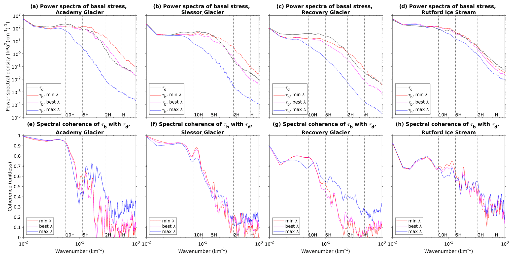
Figure 5Spectral analysis for all four detail regions highlighted in Fig. 4. Top row (a–d) shows power spectral density of basal stress (τ). Colored lines indicate spectra for minimum acceptable, maximum acceptable, and best λ values, while black lines indicate spectra for driving stress in the flow direction. Bottom row (e–h) shows coherence between basal stress τb and driving stress τd. Vertical dashed lines in all plots indicate wavelengths for select multiples of the local average ice thickness.
We show the results of this spectral analysis of basal drag for the four detail regions in Fig. 5. We have organized the regions in order of visual “ribiness”, from Academy (Fig. 5a, e) to Rutford (Fig. 5d, h). All four glaciers have roughly constant spectral power in the λmin and λbest inversions from wavelengths of about 30 to 5 H. Below 5 H, spectral power decays rapidly, while for the λmax inversion, the decay begins just above 10 H. The three most “ribby” glaciers have large differences in spectral power as a function of λ at short wavelengths, especially when comparing λmax to the other two (Fig. 5a–c), while Rutford has comparatively small differences as a function of λ (Fig. 5d). For all glaciers, the largest spread in spectral power between λmin and λmax occurs at a wavelength of about twice the ice thickness; for Academy Glacier the difference between λmin and λmax is about 3 orders of magnitude at this wavelength, while for Rutford Ice Stream the difference is less than 1. For Academy and Slessor glaciers, the λmin inversion actually has about an order of magnitude more spectral power than the driving stress at this wavelength, and λmin remains above the driving stress for all wavelengths less than 4–5 H (Fig. 5a, b). However, λbest has less spectral power than the driving stress at most wavelengths and analysis regions, only slightly exceeding the spectral power in driving stress for Academy and Slessor glaciers near a wavelength of 2 H (Fig. 5a–d). Academy and Slessor glaciers also have very high (≳90 %) coherence values between τb and τd at long wavelengths but a steep drop in coherence towards shorter wavelengths (Fig. 5e,f). This indicates that, in the “ribby” regions, driving stress and basal drag are almost fully balanced at scales greater than about 10 ice thicknesses, but this balance drops rapidly at scales of 5× or 2× the ice thickness. Thus, many of the high-resolution ribs revealed by the inversion in these regions are not mere copies of structure observable in the driving stress; the inversion adds value by revealing structure that cannot be easily inferred from ice sheet geometry. In Recovery Glacier and Rutford Ice Stream, by contrast, the gradient in coherence between long and short wavelengths is weaker (Fig. 5g, h), with values of ∼75 % even at wavelengths much larger than 10 H. This is probably a reflection of stress transmission in those glaciers, in which fast-flowing trunks with nearly zero basal drag are supported by long-distance stress transmission to shear margins or isolated sticky spots (Fig. 4d–f).
Overall, these results provide qualified support to the hypothesis advanced in Sergienko and Hindmarsh (2013) and Sergienko et al. (2014) that basal drag is often concentrated within narrow elongated ribs, at least for some of the ice streams and glaciers within our domain. Our results alone cannot confirm that the specific till-water instability mechanism they proposed is responsible for creating these ribs, but clearly some process must be invoked to explain this common spatial pattern. However, in contrast to the suggestion in those papers that the finding of ribbed structure was independent of regularization, we find that the narrow ribs are highly sensitive to the choice of λ value. Spectral analysis of our inversion results reveals that the most prominently ribbed regions also display the strongest dependence of short-wavelength structure on λ, while the least ribbed glacier we analyzed (Rutford Ice Stream) also had the weakest dependence of short-wavelength spectral power on regularization.
4.4 Resolution dependence
In Fig. 6, we show the resolution dependence of our results. As discussed in Sect. A2, we use the area-weighted median hydraulic diameter as a characteristic element size for our refined meshes, and we here restrict our analysis to element size in the fast-flowing part of the grounded ice sheet (). We find that, in the low-λ limit, the minimum achievable Jobs systematically rises with increasing element size, while the entire L-curve systematically shifts towards lower Jreg (Fig. 6a). That is, not only do inversions with coarse meshes produce less structure than inversions with fine meshes at equal values of λ, but in addition coarse meshes are also unable to fit the data as well as fine meshes, regardless of λ. The inferred values of λmin, λbest, and λmax all systematically drop as mesh resolution improves (Fig. 6b).
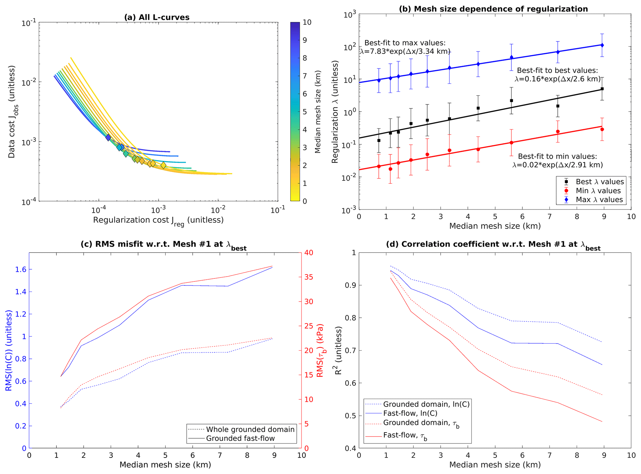
Figure 6Convergence of L-curve analysis with mesh resolution. (a) All L-curves with Weertman sliding overlain on each other. For clarity, only the fitted smooth tradeoff curves are shown, with solid diamonds marking λbest for each mesh. Curves are colored by characteristic element size. (b) Estimated values of λmin, λbest, and λmax, along with their associated uncertainties, as a function of mesh resolution. Best-fit exponentials (linear plots on the semi-logarithmic axes used here) are shown as well. (c) The rms misfit in drag coefficient (ln (C)) and drag (τb) as a function of mesh resolution. Each data point in this plot represents a comparison between λbest for a particular mesh with λbest in mesh no. 1. Solid lines represent the fast-flow domain (); dashed lines represent the entire grounded domain. (d) As (c), but showing correlation coefficients instead of rms misfits. As discussed in the text, we use the area-weighted median of hydraulic diameter in moderately fast-flow regions () to represent a characteristic element size for our unstructured refined meshes.
The dependence of all three λ values on element size is well fit by an exponential function, indicating that our results are converging towards the following non-zero λ values in the continuous solution: λmin=0.02, λbest=0.16, and λmax=7.8. Because we normalized our cost function components before combining them, we can interpret these λ values as “small”: at least for high-resolution meshes, our best estimate is that the regularization term only needs to be weighted about as strongly as the data term. The slope of the fit can be described by the e-folding element size, which is about 2–3 km for all three λ values (Fig. 6b). This length scale is comparable to the average ice thickness in our domain of 2 km. It is also comparable to the finest common flight line spacing of the radar data that were used to generate the bed topography dataset (Morlighem et al., 2020); below this length scale we would not expect our mesh to resolve substantially new features in the ice geometry. It is likely that both of these factors contribute to setting the e-folding element size. Once mesh resolution is finer than this scale, diminishing marginal returns set in, λbest approaches its limiting value, and further improvements in resolution will not allow the inversion to resolve finer structure.
In addition to examining variation in λ values, we would also like to explore the convergence of our inversion results themselves. We obviously do not have the continuous solution to compare our results with, but we can estimate an approximate picture by comparing our inversion results for λbest in each mesh with the inversion results in mesh no. 1 (Fig. 6c, d). This comparison reveals that misfits for the entire grounded domain are lower (Fig. 6c), and correlations higher (Fig. 6d), than for the fast-flow domain alone. This is likely because the spatial structure of the entire domain is dominated by the large-scale structure of streaming flow (Fig. 4), which is resolved even in the coarsest mesh we used, while restricting our analysis to the fast-flow domain represents a more difficult test of model convergence. The rms misfits for ln (C) and τb track each other closely, with values for the fast-flow domain in the range of 0.6–1.6 for ln (C) and 15–35 kPa for τb (Fig. 6c). However, correlation R2 values are consistently higher for ln (C) than for τb (Fig. 6d).
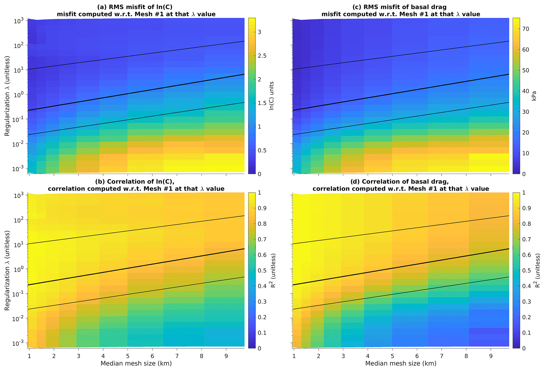
Figure 7Comparison of inversion results as a function of mesh resolution and λ value. In these plots, each inverted C or τb field is compared to the corresponding field at the same λ value at the highest-resolution mesh. Left column (a, c) shows comparison of drag coefficient C, while right column (b, d) shows comparison of drag τb. Top row (a, b) shows rms misfit, while bottom row (c, d) shows squared correlation coefficient. Best-fit lines from Fig. 6b overlain for comparison. Comparisons are limited to moderately fast-flowing regions ().
In addition to comparing inversion results at the (variable) λbest for each mesh, we can also compare our results with mesh no. 1 at a constant λ value (Fig. 7). This comparison is useful because inversions with different meshes but the same λ value should, in principle, be solving the exact same set of equations, and so any differences can be treated as model error (in practice the ice sheet geometry and surface velocity data must be filtered at different wavelengths for each mesh as described in Sect. A3, so different meshes are not solving quite the same problem). We overlay our exponential fits from Fig. 6b for reference. Above the line representing λbest, misfit in both ln (C) (Fig. 7a) and τb (Fig. 7b) is low, with only a weak dependence on λ, while correlation in both of those parameters is high (Fig. 7c, d). Between the lines representing λbest and λmin, misfit begins to rise (Fig. 7a, b) and correlation begins to drop (Fig. 7c, d), and below λmin both fit metrics worsen rapidly.
These results confirm the utility of L-curve analysis, by demonstrating that the fine structure obtained by the inversion at λbest is robust to changes in mesh resolution. There are two ways to add fine structure to the inversion results: reducing mesh size and reducing regularization. Higher-resolution meshes benefit from both improved numerical convergence and from being forced by higher-resolution geometry and velocity data, allowing them to resolve finer structure at the ice sheet bed. However, reducing λ with mesh resolution held constant will also cause the inversion to add more fine structure and reduce the observational misfit. Thus, the important question is the following: if we are limited to a coarse-resolution mesh, at what point does the fine structure obtained by reducing regularization diverge from the fine structure we would have obtained if we were able to use a finer mesh? L-curve analysis is a test that can be performed on a single mesh without reference to inversions on finer meshes. The results shown in Fig. 7 demonstrate that the fine structure obtained by reducing regularization begins to diverge from the fine structure obtained by improving resolution below λbest, and below λmin the difference between the two increases rapidly.
4.5 Effective pressure
Before analyzing our results for Budd sliding in detail, it is useful to consider Eq. (4): in order to reproduce the stress and velocity fields recovered by the Weertman inversion, the Budd coefficient must satisfy the relationship CW=CBN, where CW is the coefficient in the Weertman sliding law and CB is the coefficient in the Budd sliding law. From this, we can form the a priori expectation that the utility of a given N field will be dependent on the linear correlation between N and CW. If N has a strong positive correlation with CW, then the inversion will not need to produce much structure in CB in order to fit the observations; in the limit of a perfect N field and no material variation in the substrate, the N field would explain all of the variation in CW, and CB would be a constant. Conversely, if the correlation between N and CW is weak or even negative, then the inversion will need to produce a lot of structure in CB in order to fit the observations.
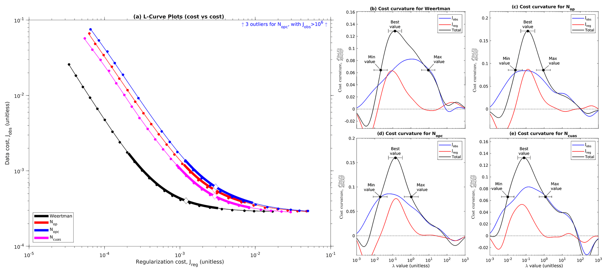
Figure 8Comparative L-curves for different N fields. (a) All L-curves overlain on each other. Small circles represent individual models, thin lines represent smoothed curves, thick lines represent inferred corner regions, and large diamonds represent inferred λbest values. (b–d) Cost curvature as a function of λ for each N field, with selection of minimum, best, and maximum λ values annotated. Plot (a) is equivalent to plot (a) in Fig. 3; plots (b–d) are equivalent to plot (d) in that figure. Three outlier models from Nopc have been excluded from this analysis.
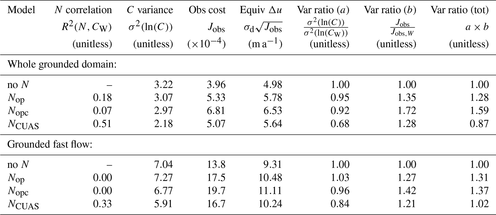
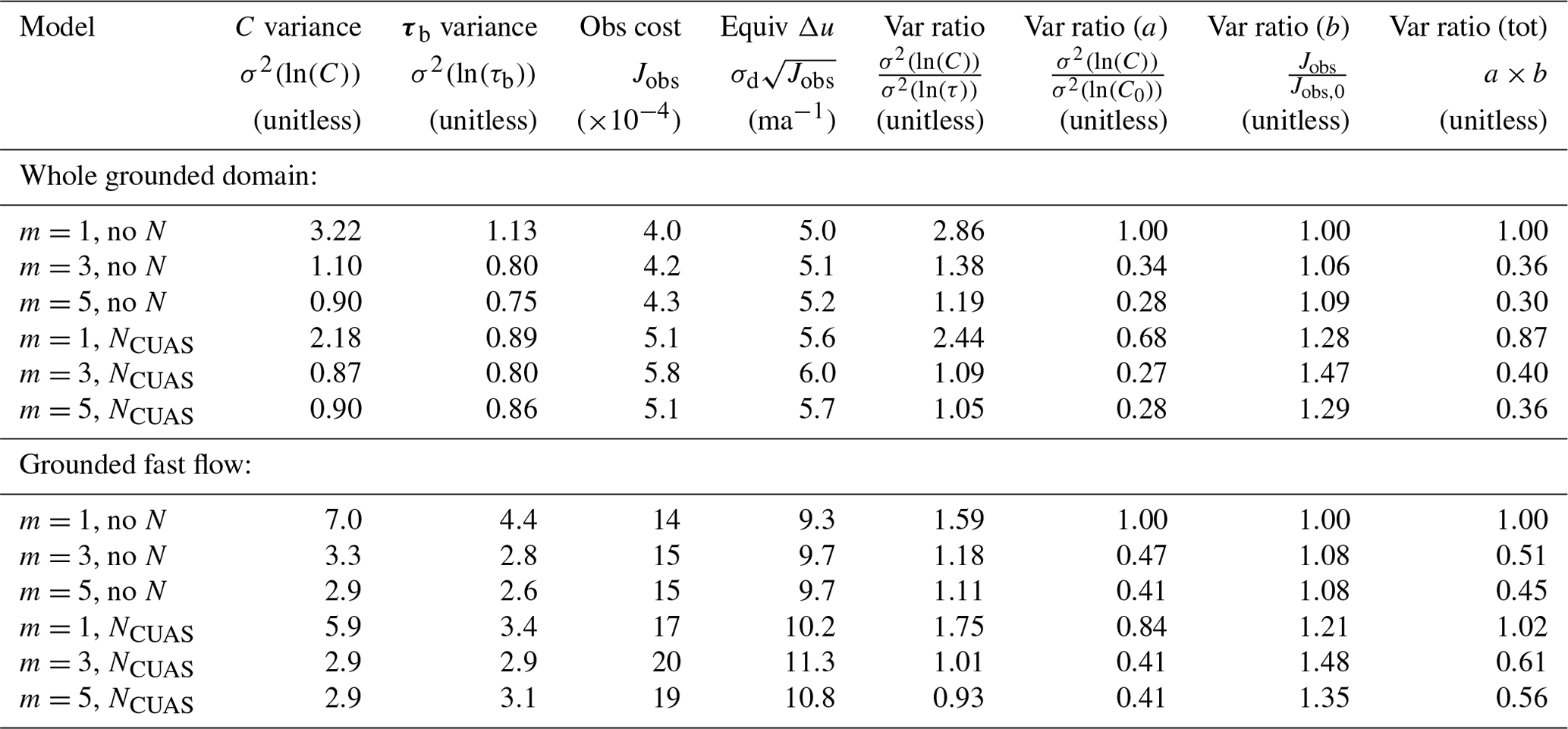
All three of our candidate N fields had a positive correlation with CW, but NCUAS had much better correlation than either of the two geometry-based N fields (Table 1). In addition, all three N fields had better correlation values when considering the entire grounded domain than when considering the fast-flow region alone (Table 1). For the geometry-based N fields, this is likely due to the physical setting of fast-flowing regions: many fast-flowing ice streams and outlet glaciers are located in subglacial troughs, so a simple geometry-based calculation incorporating the bed topography can approximate the basic dichotomy between slow flow and fast flow. For NCUAS, this is likely because the melt rate forcing to CUAS incorporated shear heating estimated from the observed velocity field. Restricting the analysis to the fast-flowing region alone represents a much more stringent test; NCUAS can explain 33 % of the variance of CW within the fast-flowing region of the domain, but the two geometry-based N fields can explain almost none of it.
Figure 8 shows comparative L-curves for all of them, and Table 1 summarizes the results of a comparison between the λbest inversions for each of those N fields with the λbest inversion for Weertman sliding. The L-curves for all three N fields have a similar shape as the L-curve for Weertman sliding but shifted towards higher Jreg (Fig. 8a). Total curvature was in the range of 0.13–0.17 for all four models (Fig. 8b–e), providing a quantitative confirmation of the visual similarity in shape. The inferred λbest values are shifted towards lower λ values, mostly driven by a shift in the data curvature term (Fig. 8c–e, cf. b). A visual inspection of the respective L-curves suggests that the asymptotic best achievable Jobs is similar for all sliding laws, but the λbest inversions for inversions with N have higher Jobs than the λbest inversion for Weertman sliding (Fig. 8a). Three of the inversions in the Nopc L-curve were unable to converge, with Jobs many orders of magnitude higher than the other models (Fig. 8a), but the remaining inversions were sufficient for us to recover a smooth tradeoff curve.
At face value, Fig. 8a implies that Nopc required the most structure to fit the data, almost a full order of magnitude more structure than the inversions with Weertman sliding. However, it is possible that the increase in Jreg could have been caused by the different normalization used, as the estimate of the characteristic scale Sreg depends on the value of N (Eqs. 11, 14). To remedy this, we can obtain a scale-independent estimate of the magnitude of the structure produced by the inversion by computing the variance of ln (C). Converting C to a logarithmic scale before computing the variance ensures that the change in units and mean magnitude between Weertman and Budd sliding has no effect on the calculation. This calculation reveals that all of the candidate N fields reduced the variance in the inverted C coefficient when considered over the entire domain, but NCUAS reduced the variance the most (Table 1). When the fast-flow domain is considered alone, Nop produced a slight increase in variance, Nopc a slight decrease, and NCUAS the largest decrease. All of the inversions with N had larger Jobs values than the inversion with Weertman sliding, regardless of whether or not the analysis is restricted to the fast-flow domain, with NCUAS having the smallest increase in observational misfit of the three (Table 1). In addition, the scaling of Jobs is determined only by the statistics of the observations (Eq. 13), so we know that differences in Jobs between models are directly comparable with one another. Nonetheless, the absolute magnitude of error for all of the models is relatively low, with over the whole domain and over the fast-flow region; converted back to dimensional form using , these correspond to characteristic velocity errors of over the whole domain and in the fast flow. We can evaluate the overall quality of each model by computing the total variance ratio, which is the product of the coefficient variance ratio and the Jobs ratio (Table 1). Doing so reveals that the increase in observational misfit outweighs the reduction in coefficient variance for the two geometry-based N fields (Nop and Nopc) regardless of whether the analysis is performed for the whole domain or for the fast-flow alone; for NCUAS, by contrast, we obtain a reduction in total variance for the whole domain and a very slight increase in the fast flow.
Table 1This table summarizes inversion performance for the three sources of effective pressure N that we tested on mesh no. 1, alongside results for Weertman sliding (no N). Each model is evaluated at its own λbest value. We show statistics both for the entire grounded domain and for fast-flow regions only ().
4.6 Nonlinear sliding
In Fig. 9, we show comparative L-curves for linear and nonlinear Weertman sliding laws. These results reveal that, in a nonlinear sliding law, the high-λ limb of the L-curve is substantially steeper than in a linear sliding law, producing a sharper corner in the L-curve (Fig. 9a). The peak in cost curvature became narrower as sliding became more nonlinear, reducing the spread between λmin and λmax and allowing us to define the corner region more precisely (Fig. 9c, e, g). The increased visual sharpness of the L-curves for nonlinear sliding can be confirmed by looking at the total curvature, which doubles from 0.13 for m=1 to 0.26 for m=5 (Fig. 9c, e, g). The increase in L-curve sharpness for nonlinear sliding is driven by both a steeper increase in Jobs and a shallower reduction in Jreg with increasing λ (Fig. 9b, d, f). Both of these effects can be explained by an increasing sensitivity of velocity to the coefficient in nonlinear sliding. Rearranging Eq. (3) to solve for u reveals that ; thus, when C is perturbed away from a value that fits the observations closely, the resulting increase in Jobs will be larger for nonlinear sliding than for linear sliding. The increased sensitivity of Jobs to C in turn prevented the inversion from smoothing C as much as it would for linear sliding, producing higher Jreg values at large λ. The combination of a smaller decrease in Jreg with a bigger increase in Jobs at large λ produces a sharper L-curve.
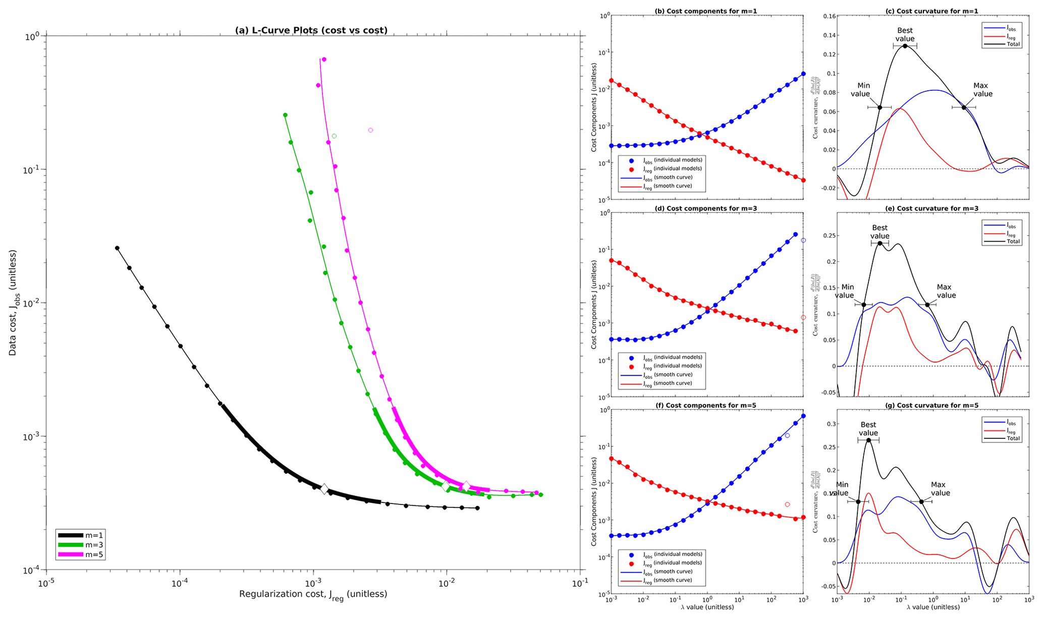
Figure 9Comparative L-curves for different values of the sliding exponent m in mesh no. 1. (a) All L-curves overlain on each other. Filled circles represent individual models, thin lines represent smoothed curves, thick lines represent inferred corner regions, and large diamonds represent inferred λbest values. Open circles represent two outlier models excluded from the curve-fitting (one each for m=3 and m=5). (b) Individual cost components for m=1. Filled circles represent individual models, lines represent fitted curves, and open circles represent outlier models. (c) Cost curvature and selection of λmin, λbest, and λmax for m=1. (d–g) As (b) and (c) but for m=3 and m=5.
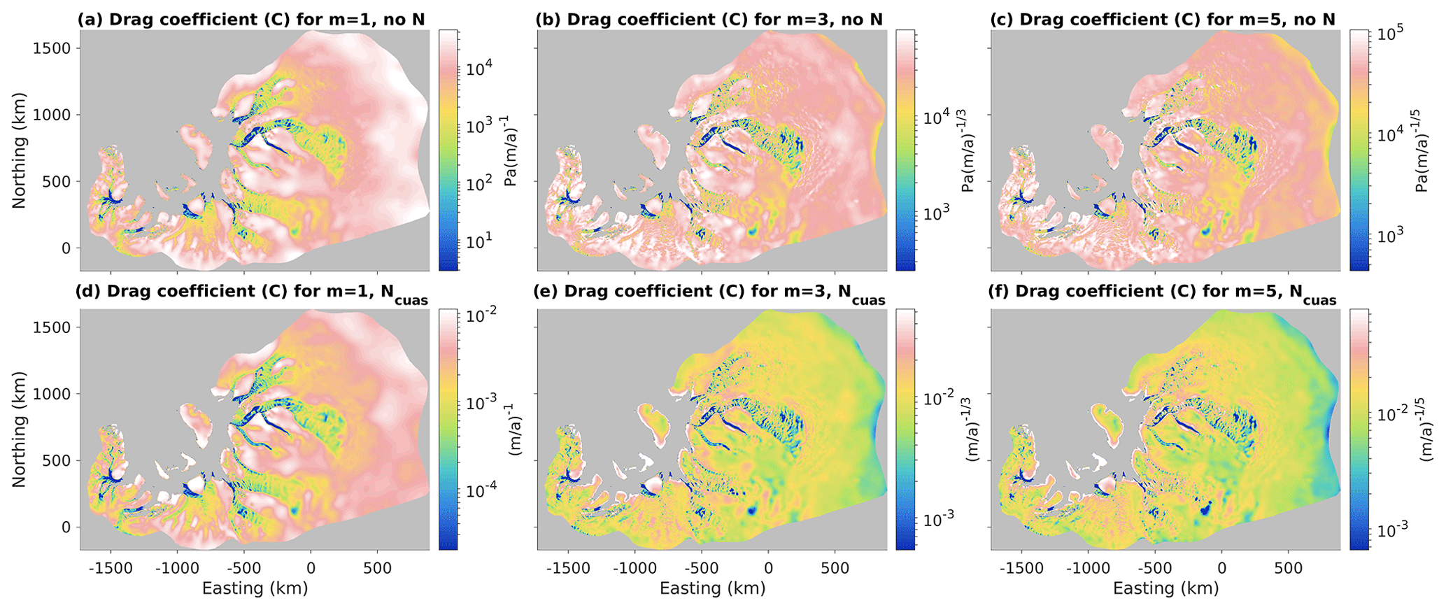
Figure 10Comparative maps of inverted drag coefficient C for different values of the sliding exponent m, both with and without effective pressure N. Top row shows drag coefficient for Weertman sliding (without N), for . Bottom row shows the same values of m for inversions with Budd sliding using NCUAS. Each subplot uses a logarithmic color scale with the limits automatically set to the 1st and 99th percentiles of the distribution.
As in our experiments with N, a first glance at our L-curves in Fig. 9a seems to imply greater inversion structure with higher values of m. However, again care needs to be taken when interpreting Jreg, as the scaling of Jreg depends on the value of m (Eq. 11). Again, we can obtain a scale-independent estimate of the amount of structure present in the inverted field by computing the variance of ln (C). Doing so reveals that the structure produced by the inversion drops drastically as m increases, dropping by a factor of 3–4 over the whole domain and by a factor of 2–2.5 in the fast flow (Table 2). This reduction in variance can also be seen by examining the color scales in Fig. 10. At the high end, linear Weertman requires over 5.5 orders of magnitude of dynamic range to display the 1 %–99 % range of its distribution, while at the low end, nonlinear Budd requires less than 2.5 orders of magnitude. The spatial structure of C also changes somewhat in nonlinear sliding, with greater ribbing and less of a simple dichotomy between fast and slow regions, producing a C field that starts to have more visual features of the τb field for linear sliding (Fig. 10b, c, cf. Fig. 4d–f). With nonlinear Budd sliding the large-scale contrast between slow and fast flow is greatly reduced, with much of that distinction being accounted for by NCUAS rather than C (Fig. 10e, f). The coefficient variance can also be compared with the variance of ln (τb), as we expect that C→τb as m→∞. For linear Weertman, the variance in the coefficient is nearly 3 times the variance in basal drag when considered over the whole domain, but this drops to only a 20 % increase in variance for m=5. For NCUAS with m=5, the coefficient variance is only 5 % higher than the drag variance over the whole domain, and it is actually 7 % less in the fast flow. Observational misfit is slightly higher for nonlinear as compared to linear sliding, although as with our experiments with N, the absolute magnitude of Jobs is low for all inversions and the equivalent velocity errors are on the order of for the whole domain and in the fast flow. However, unlike in our experiments with N, for our experiments with m the large reduction in coefficient variance moving to nonlinear sliding more than makes up for the slight increase in misfit, producing total variance ratios that are an unambiguous improvement (Table 2). The improvement produced by moving from m=1 to m>1 in Weertman sliding is about a factor of 3 when measured across the whole domain, and about a factor of 2 within the fast flow. m=5 produced a slight improvement as compared to m=3, but by far the biggest jump came between m=1 and m=3. With NCUAS the improvement when moving from linear to nonlinear sliding was somewhat less, although still strong (Table 2).
Table 2This table summarizes inversion performance for the three values of the sliding exponent m that we considered in mesh no. 1. Each m is evaluated at its own λbest value. C0, the drag coefficient used for comparison with the other models, is the reference model (m=1, no N). We show statistics both for the entire grounded domain and for fast-flow regions only ().
4.7 Higher-order inversions
We produced L-curves for HO inversions with linear Weertman sliding in mesh nos. 4, 6, and 8. We compare these with the corresponding SSA inversions in Fig. 11. While we were able to obtain smooth monotonic L-curves with well-defined corner regions for all three experiments, the resulting L-curves clearly indicate that the HO inversions were inferior to SSA inversions using the same mesh and sliding law. Note that the scalings for both Jreg and Jobs are independent of the flow equation used, so the relative positions of the SSA and HO L-curves in Fig. 11 are directly comparable to one another. This positioning indicates that the HO inversions performed worse than the SSA inversions in both components of the cost function. The difference in the asymptotic best achievable Jobs is particularly notable: the HO inversions were incapable of achieving values of Jobs less than 10−3, regardless of mesh resolution. By contrast, the asymptotic best achievable Jobs for the SSA inversions improved with finer mesh resolution, as discussed above.
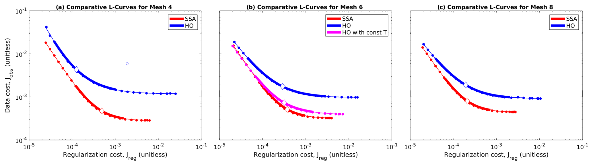
Figure 11Comparative L-curves for HO and SSA inversions. (a) Comparative L-curves for mesh no. 4. Solid circles indicate model results, thin smooth lines indicate fitted curves, thick lines indicate corner region, diamonds indicate λbest location, and hollow circle indicates an outlier model excluded from the curve-fitting for HO. Red represents SSA L-curve; blue represents HO. (b) As (a) but for mesh no. 6. Magenta represents HO with constant ice temperature of −25 ∘C. (c) As (a) but for mesh no. 8.
A detailed examination of the misfit maps for the HO inversions (not shown) revealed that their increased observational misfit was largely due to increased positive misfit (i.e., model velocity too high) in slow-flowing regions. Thus, we hypothesized that they may have been unable to fit the data because they contained too much deformation flow: if the temperature model used as input contained too much warm ice near the base, then a vertically resolved HO model would have too much shear deformation in the lower part of the ice column, resulting in model surface velocities that were faster than observed, with no way to bring the model velocities down by adjusting basal slip. We tested this hypothesis by running one additional L-curve experiment in mesh no. 6 with HO and a constant ice rheology corresponding to a temperature of −25 ∘C throughout the domain. The results are shown by the magenta line in Fig. 11b. With a constant, and fairly stiff, ice rheology, this HO model was able to make up almost all of the difference with the SSA L-curve.
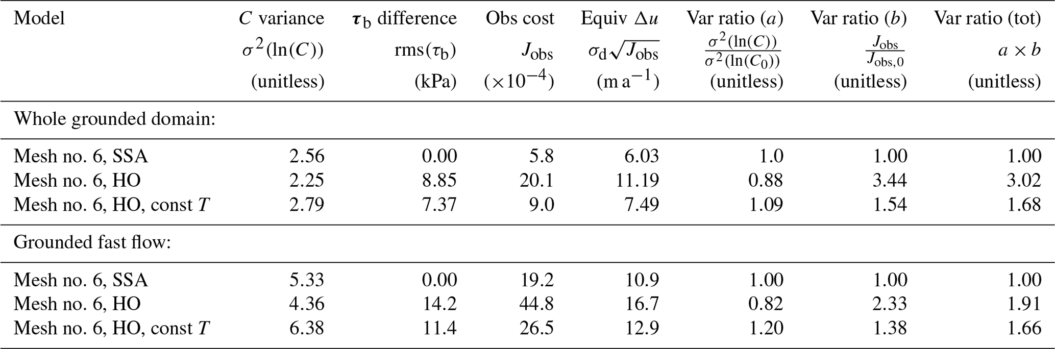
We summarize the performance of the two HO inversions in mesh no. 6 as compared to the SSA inversion for that mesh in Table 3. Basal drag was similar in both the 2D and 3D models, with rms differences in τb on the order of 10 kPa. The HO model with variable ice temperature required more regularization and thus had 12 % less variance in its coefficient than the SSA model, but it also had a big increase in Jobs, resulting in a tripling in the total variance ratio (Table 3). The HO inversion with constant ice temperature performed better than this but still had a 68 % increase in total variance as compared to SSA. When the analysis is restricted to the fast-flowing domain, then the HO inversion with variable temperature improves somewhat, dropping down to a variance ratio compared to SSA of “only” 1.91, while the variance ratio for HO with constant temperature is nearly identical within the fast flow as it is in the whole domain (Table 3). These results demonstrate that, while SSA outperforms HO regardless of whether the analysis is performed over the whole domain or in the fast flow alone, the SSA model has the biggest advantage when compared against the HO model with variable temperature in a comparison region that includes both slow and fast flow. We discuss our interpretation of these results in more detail in Sect. 5.3.
Table 3This table summarizes inversion performance for HO and SSA models in mesh no. 6. Each model is evaluated at its own λbest value. Variance ratios and basal drag differences are computed with respect to the SSA model. We show statistics both for the entire grounded domain and for fast-flow regions only ().
4.8 Best drag map
Throughout this paper we have produced many different inversions and competing descriptions of the ice sheet basal drag. In this subsection, we combine them to produce a single consensus picture representing our best combined estimate. We feel that it is more appropriate to produce a consensus view of drag, τb, rather than drag coefficient C, because drag is directly comparable between different sliding laws, while the units and mean magnitude of C vary with both m and N. In this consensus estimate we include all eight of the L-curves that we performed on our highest resolution mesh, that is, Weertman sliding with , Budd sliding with NCUAS and the same three m values, and linear Budd sliding with NOP and NOPC. In order to sample the range of uncertainty associated with regularization, for each L-curve we included inversions with λmin, λbest, and λmax. Overall, our combined estimate is built from 24 individual inversions on our highest resolution mesh. Each inversion is weighted according to the inverse of its total variance ratio. For this purpose we use the value of total variance computed for the whole domain. We estimated the uncertainty in this combined drag map by computing the weighted standard deviation of these 24 inversions about the mean field using the same weighting.
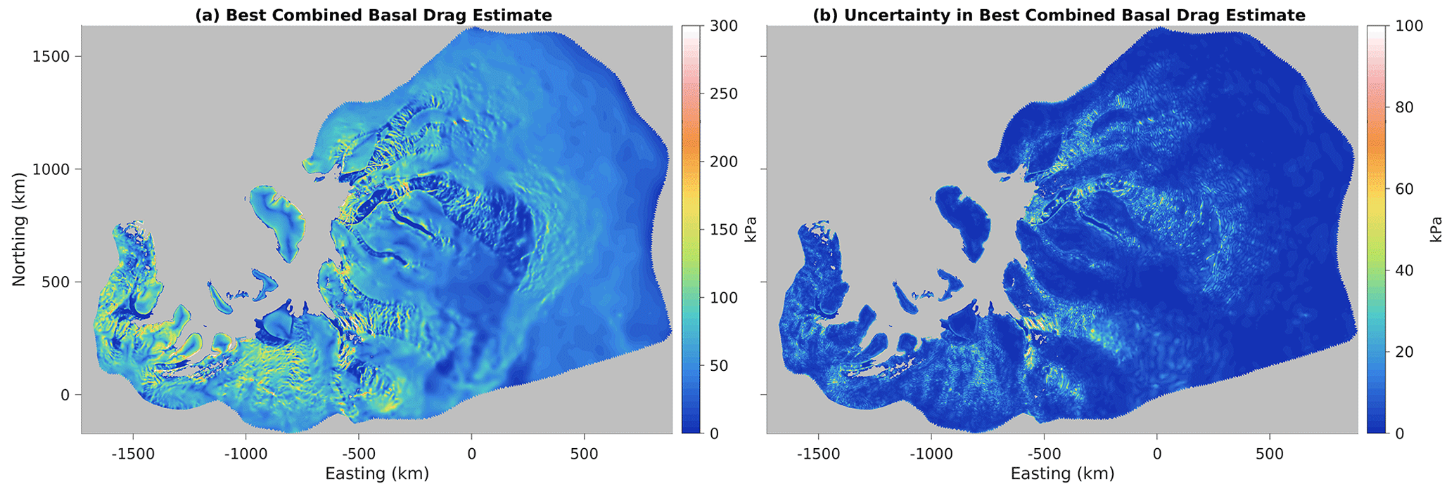
Figure 12Our best combined estimate of the ice sheet basal drag (a) and its uncertainty (b). This map is produced by taking a weighted average of multiple models as described in the text. The uncertainty is computed from the weighted standard deviation. Each model is weighted by the reciprocal of its total variance ratio.
Figure 12a shows the resulting spatial structure of basal drag. A number of faster-flowing regions are supported by rib-like structures in drag, including upstream Recovery and Slessor glaciers, Academy glacier, and the region of the Robin Subglacial Basin upstream of Institute and Möller ice streams. Generally these ribby regions are further upstream in the fast flow, while further downstream many fast-flowing trunks have nearly zero basal drag supported by stress transmission from shear margins or isolated sticky spots. Fast-flowing trunks with mostly zero basal drag are seen in Recovery and its tributaries, Rutford, Evans, and Foundation and downstream Slessor glaciers. Stress transmission from fast-flowing trunks to the shear margins produces thin strips of high drag just outside of the main trunk of many glaciers. In general, more visually ribby structure tends to be located in moderately fast-flow regions, ∼30–300 m a−1, where streaming flow is spread out over broad subglacial basins. Where fast flow is more intense () and concentrated in narrower troughs, the tendency is towards near-zero basal drag supported by isolated sticky spots or side drag from shear margins. Recovery and Support Force glaciers have regions of high drag near their grounding lines, but otherwise most glaciers continue their low-drag troughs right into the ice shelf.
The uncertainty in our combined drag estimate is mostly low, but with large excursions co-located with areas of high drag (Fig. 12b). The mean uncertainty is 5.5 kPa in the whole grounded domain and 12.6 kPa in the fast-flowing region. In general, high-drag ribs and shear margins tend to also have higher uncertainty, especially in the fast-flowing part of the domain, while the weak-bedded trunks of glaciers have low uncertainty (Fig. 12b). The apparent visual correlation between mean drag and drag error can be confirmed by fitting a linear relationship between them with the constraint that the fitted relationship must pass through the origin; doing so reveals that drag uncertainty is 11 % of the mean drag over the whole domain and 18 % of the mean in the fast flow, with R2 values for these relationships of 0.53 and 0.66, respectively.
Fundamentally, the purpose of regularization is to determine the information content of our observations by managing the tradeoff between increased complexity in the inversion target field and reduced observational misfit. While one can usually reduce the observational misfit by adding ever more complexity to the inversion target field, this is equivalent to increasing the number of free parameters one is allowed to tune, and the meaningfulness of a good observational fit achieved with an excess of free parameters is questionable. Occam's razor suggests that we should prefer the model that explains the maximum amount of observational variance with the minimum amount of spatial structure. The ideal λ value is thus defined by the point of diminishing marginal returns: starting from a highly regularized state, reducing λ improves the observational fit substantially without adding much spatial structure to the target field. At some point, diminishing marginal returns set in, such that further improvements require disproportionately complex spatial structure in the target field to achieve only slight reductions in misfit. Thus, regularization is not an ad hoc or arbitrary addition to the inversion process, nor should regularization be treated as an inconvenient or unfortunate necessity required to produce numerical stability. Rather, regularization is a fundamental measure of the information content achievable in geophysical inverse problems, and the selection of optimal regularization should be regarded as an essential part of glaciological inversions. A well-formed L-curve allows us to answer the following question: how much structure is actually required to fit the data? Conversely, a poorly formed L-curve casts doubt on the meaningfulness of all of the spatial structure recovered by an inversion.
This focus on information content also provides a useful framework for thinking about the question of convergence in inverse models. In forward models, “convergence” can be simply defined to mean that, in the limit that mesh resolution approaches zero, the numerical solution approaches the continuous solution. In inverse models, by contrast, there are two fields that the numerical solution could potentially approach: the continuous solution and the true field. If the true field is sufficiently rough in comparison to the attenuating effect of the forward problem, then the limit of λbest will not be 0, and the continuous solution of the regularized inverse problem will not be the same as the true field (Vogel, 1996). This split is also reflected in the fact that, for inverse problems, we must formally consider “convergence” with respect to multiple limits: the limit as model resolution approaches zero, the limit as observational error approaches zero, and the limit as observational resolution approaches zero. In our resolution tests (Sect. 4.4), we explored the convergence behavior with respect to both model and observational resolution (because we smoothed the observations onto coarser meshes, Sect. A3), but not convergence behavior with respect to observational error. We found that λbest approached a non-zero limit, implying that (at least with non-zero observational error) the continuous problem would require non-zero regularization and therefore the continuous solution of the inverse problem should differ from the true basal drag.
If it is not the true basal drag, what then is the continuous solution? It is useful to think of the continuous solution of the regularized inverse problem as the best knowable drag field. When λbest approaches a non-zero limit, as we found, then the best knowable drag field is not the same as the true drag field, although it is related to the true field through a low-pass filtering operation: the best knowable field is the true field filtered for the components that have a detectable influence on the observations. For any given non-zero resolution of mesh and observations, the corner of the L-curve gives the most amount of structure that can be reliably inferred at that resolution, and taking the limit as resolution approaches zero gives the most amount of structure that can be reliably inferred from observations of that precision. It remains to be seen whether the best knowable field approaches the true field in the limit that observational error also approaches zero.
5.1 Sliding nonlinearity
It is common in the inverse modeling literature to read some version of the statement that, because it is possible to fit the data and achieve force balance with any sliding law, we therefore cannot use inverse models to distinguish between different sliding laws. For instance, Joughin et al. (2004) state that “the inversion results alone do not distinguish which is the most appropriate bed model”, wording which is repeated almost verbatim in Joughin et al. (2006). Under this logic, inverse models can only be used to discriminate between different sliding laws if they have access to time-dependent information, either by simultaneously fitting data from multiple time slices with a single coefficient field (Gillet-Chaulet et al., 2016) or by evaluating the ability of transient models forced by different sliding laws to fit time-dependent geometry and velocity data (Joughin et al., 2010a). Inversions of a single time slice are thought to be neutral between different sliding laws, so long as all of the competing sliding laws obtain a similar fit to the data.
However, we argue that inverse models are not neutral between different sliding laws, even if they are limited to a single time slice. Occam's razor dictates that, when choosing between two parameterizations that both obtain a similar fit to the data, we should prefer the parameterization that requires less complexity to do so. In the case of a sliding law, we are creating a parameterization that relates two quantities that each have about 2–3 orders of magnitude of dynamic range: velocity varies between about 1 to about 1000 m a−1, and basal drag varies between a few kilopascals and a few hundred kilopascals. Yet we found that linear Weertman sliding requires a coefficient with twice as much dynamic range as either of those two parameters. This result is not exactly new or controversial. Almost all published inversions of real data with linear sliding laws require many orders of magnitude of dynamic range in C (e.g., Arthern et al., 2015, Fig. 7). Indeed, this result is so well-known in the glaciological modeling community that it has been incorporated into the design of some models: for example, Elmer/Ice uses α=log 10(C) as the free parameter in their inversions rather than C itself (Gagliardini et al., 2013). However, it is less common for glaciologists to reflect on what this result means for the utility of linear Weertman sliding. Good parameterizations help us represent complex processes by simplifying them in ways that isolate the key variables and reduce the unknowns. A sliding law that doubles the amount of unexplained variance at the ice sheet bed has fundamentally failed to be a useful parameterization.
Thus, we would argue that, rather than being agnostic about the value of the sliding exponent, inverse models actually provide evidence in favor of nonlinear sliding. Our total variance measure, which combines both observational misfit and coefficient variance, was better for nonlinear sliding as compared to linear sliding by about a factor of 3 over the whole domain or a factor of 2 when the analysis was limited to the more challenging fast-flow region. In addition, our L-curves for nonlinear sliding were more sharply curved, producing a narrower and more well-defined range of acceptable λ values. Of course, this evidence from single-snapshot inverse models is not definitive on its own; if other lines of evidence supported linear Weertman sliding, then we would be forced to accept the large variance in C as the reality. However, other lines of evidence indicate the opposite. Laboratory tests on actual samples of subglacial till consistently reveal Coulomb plastic rheology for soft basal sediments (e.g., Kamb, 1991; Tulaczyk et al., 2000). Analytical and numerical process models for hard bed sliding with cavitation show Coulomb-like behavior with basal traction bounded by a maximum yield stress (Iken, 1981; Schoof, 2007; Gagliardini et al., 2007). Transient numerical modeling of the visco-elastic response of glaciers to tidal forcing suggests that nonlinear sliding is required to fit the response recorded with GPS observations (Gudmundsson, 2011). The previously mentioned inversions of time-dependent velocity and geometry data support nonlinear sliding (Gillet-Chaulet et al., 2016), as do transient models (Joughin et al., 2010a). Thus, the evidence from single-snapshot inversions adds to a convergence of many lines of evidence indicating that the best description of basal sliding is a nonlinear one.
5.2 Effective pressure
While our inverse model results are strongly in favor of nonlinear basal sliding, they are more ambiguous on the utility of including effective pressure in a sliding rule. Other lines of evidence, including laboratory tests (Tulaczyk et al., 2000), field observations (Kamb et al., 1985; Andrews et al., 2014), and analytic and numerical process models (Iken, 1981; Schoof, 2007; Gagliardini et al., 2007), argue that basal water pressure plays an important role in regulating basal sliding. The importance of subglacial water in regulating basal sliding is by now the unambiguous consensus of the glaciological community (e.g., Cuffey and Paterson, 2010, Chap. 7). However, the question addressed by inverse models is a more subtle one: not whether basal water pressure plays a role in the real physics of ice sliding, which it undoubtedly does, but whether our models of basal water pressure are good enough to make N a useful addition to a large-scale sliding law.
When it comes to simple geometry-based calculations for N, our answer is an unequivocal no: the slight reduction in inversion variance produced by these N fields is insufficient to compensate for the increase in observational misfit, regardless of whether the analysis is performed for the whole grounded domain or for the fast-flow region alone. When it comes to the physically based NCUAS, however, our results are more ambiguous. When considered over the whole domain, using NCUAS with linear sliding reduced total variance by 13 %, but when considered in the more challenging fast-flow region alone, it increased total variance by 2 %. Both of these changes are small compared with the large reductions in total variance achieved by using m>1. Using m>1 along with NCUAS produced improvements when compared with either linear Weertman or linear Budd sliding, but not when compared with nonlinear Weertman at the same value of m (Table 2). Thus, our results do not provide support for using N in basal sliding laws – yet. If one is forced to use a linear sliding relationship, and one is mostly concerned with capturing the large-scale pattern of slow and fast flow, then our results suggest that one could improve one's model by including a physically based N field like NCUAS. However, the resulting improvement is much less than the improvement that one could get by moving from linear to nonlinear sliding, and if nonlinear sliding is combined with NCUAS, the improvement vanishes.
Nonetheless, there remains hope that further improvements in hydrological models may change the situation. NCUAS was unambiguously better than either of the two geometry-based N fields, demonstrating that the performance of inversions using Budd sliding is sensitive to the quality of the N field; it is thus reasonable to assume that further improvements in N will improve inversion performance further. Given that we found that the performance of nonlinear Budd laws with NCUAS was very close to the performance of nonlinear Weertman laws at the same value of m (within 5 %–10 %, measured in units of the total variance in the linear Weertman inversion, Table 2), it would not take much improvement for nonlinear Budd inversions to overtake nonlinear Weertman inversions. Furthermore, we know from the basic math of our sliding laws that there is a hard limit to the performance of nonlinear Weertman inversions: the coefficient in a nonlinear Weertman sliding law must always have at least as much dynamic range as the dynamic range of basal drag, which for typical ice sheet settings is at least 2 orders of magnitude. By including N, Budd sliding laws open up the possibility that the variance of the coefficient can drop below this limit, and indeed we found that in our inversion with NCUAS and m=5, the variance of the coefficient was slightly less than the variance of basal drag in the fast-flow region. The total variance for this model was still higher than for Weertman sliding with m=5 (Table 2), but the fact that one of our Budd models was able to dip below this limit is a hopeful sign that future improvements in subglacial hydrology models may explain more of the variance in basal drag. Put simply, nonlinear Weertman may be better than nonlinear Budd right now, but it also has a much lower ceiling. With m=5, nonlinear Weertman is already within 10 %–20 % of the best possible performance it can achieve, whereas sliding laws that incorporate effective pressure can be as good (or as bad) as the hydrology model they use as input.
5.3 Three-dimensional models, two-dimensional inversions
In almost all of our experiments in this paper, we used the SSA stress balance equations, which are the simplest approximation that can be used in an inversion. It is tempting to assume that inversions using more advanced stress balance equations, such as HO or full Stokes (FS), are inherently more powerful than inversions performed with the SSA equations. However, that is forward model thinking, not inverse model thinking. From an inverse modeling perspective, the extra stress and strain rate components found in HO and FS models are a liability, not an asset. If a simpler SSA model is able to obtain a similar fit to the data as a more complex HO or FS model, then it is the simpler model that should be preferred. But “similar fit” may actually be an optimistic case for the more complex models: in our experiments comparing HO and SSA using the same mesh and sliding law, we found that the SSA inversion was able to obtain a better fit to the data than the HO model. There is thus very little justification, from our results at least, for using the more complex stress balance equations in an inversion.
The proximal cause of the poor performance of our HO inversions was that the basal ice rheology was too warm in large portions of the domain. Remedying this by using a constant cold rheology at all depths throughout the domain brought the inversion performance closer to the performance of the SSA inversion. However, a spatially invariant constant is a very poor approximation of the ice sheet thermal structure; it ignores very real variations in thermal boundary conditions such as surface temperature, accumulation rate, geothermal flux, ice thickness, and strain heating. While we probably could have produced a realistic colder temperature field that enabled our HO inversions to match the performance of our SSA inversions with a bit of work, the mere fact that this tuning is required is a mark against the HO inversions. In addition, using a stiffer ice rheology near the bed has the effect of greatly reducing shear deformation, forcing the entire domain to shift towards a regime of plug flow. In other words, in order to improve the performance of our HO inversion, we had to force it into a regime where it mimicked SSA! This explanation may also help to explain why some previous studies, such as Shapero et al. (2016), have found that the results of 3D inversions were insensitive to ice rheology. In that study, the authors performed FS inversions in restricted domains around three of the largest and fastest outlet glaciers in Greenland: Jakobshavn, Helheim, and Kangerdlugssuaq. While they did include a small amount of stagnant ice around the margins, the overwhelming majority of their three domains were composed of ice moving at least several hundred meters per year, which usually indicates that flow is dominated by basal slip, or at least, that they are unlikely to be in the regime where slip has dropped to zero and the sliding inversion is powerless to reduce velocity further. While Shapero et al. (2016) did not compare the performance of their FS inversion with an SSA inversion, our prediction would be that, if they had performed a comparative L-curve analysis, they probably would have found that their FS inversion had roughly the same performance as an SSA inversion.
Fundamentally, the problem is that, by allowing for vertical variations in rheology, strain rate, and therefore velocity, HO and FS introduce an enormous amount of variability into the problem that cannot be constrained by the available datasets. Sliding inversions typically take the rheological structure of the ice sheet to be fixed, but properly speaking, an FS or HO inversion should be simultaneously adjusting the sliding coefficient and the rheology of the lower ice column. While glaciological inversions for vertically averaged rheology have been performed (e.g., Larour et al., 2005), we are not aware of any cases of glaciologists performing mechanical inversions for vertically resolved rheology. This is unsurprising, because the data we use to constrain ice sheet inverse models are essentially two-dimensional: we have maps of the two components of horizontal velocity on the upper surface of the ice sheet. If the rheology of the lower ice column is soft enough to permit a deformation velocity greater than the observed surface velocity, then an HO or FS inversion has no remedy to fix this by adjusting sliding, and it will be incapable of fitting the data. Conversely, if the rheology of the lower ice column is too stiff to permit a rapid deformation velocity, then the ice sheet will move primarily by plug flow and the HO or FS inversion will merely recover the same performance that could have been achieved by an SSA inversion with far less internal complexity. In the absence of any constraint on variation in the third dimension, a two-dimensional SSA model works best because it is a match to the two-dimensional nature of the data.
It is interesting that we found that our SSA inversions even outperformed our HO inversions in slow-flowing areas of the ice sheet, where the SSA equations should not be a good approximation to the ice sheet stress balance. However, this is less surprising when considering the framework of the “hybrid” approximation to the stress balance equations (Schoof and Hindmarsh, 2010; Goldberg, 2011). In this approximation, shear deformation in the lower ice column is parameterized as a component of the sliding law, with ice velocity being decomposed into the sum of sliding and deformation flow, and basal drag being determined by whichever process (slip or deformation) is weaker. Crucially, the vertically integrated stress balance equations of this approximation are identical to the SSA equations; the only difference is that the effective viscosity computation is modified to include the contribution of vertical shear to the effective strain rate, and the sliding law is modified to reflect the fact that resistance to flow could come from shear deformation in the lower ice column instead of sliding over the bed. The hybrid approximation applies throughout the ice sheet, not merely in fast-flowing streams and shelves moving by plug flow, and because its stress balance equations are identical to those of SSA, an SSA inversion can therefore be regarded as representing a smooth transition between a sliding inversion in fast-flowing areas and an inversion for near-basal rheology in slow-flowing areas. Under this framework, our SSA inversion results for drag coefficient in slow-flowing regions could be reinterpreted as a measure of the integrated stiffness of the lower ice column rather than as a measure of sliding itself. But regardless of how we choose to interpret our results, the SSA equations themselves are agnostic as to whether the resistance to horizontal flow comes from slip across the basal interface or from shear deformation a short distance above, and this very agnosticism is the key to their success at fitting surface velocity data, which cannot distinguish between sliding and deformation either.
On the basis of the results and discussion above, we suggest the following principles for guiding the use and analysis of L-curves for regularization in glaciological inversions. Note that, while we have made a number of particular choices in our model setup here (e.g., the choice to use the L2 norm of absolute velocity misfit for Jobs), these recommendations apply for any use of L-curve analysis in glaciological inverse modeling.
-
Whenever possible, modelers should use an a priori estimate of characteristic scale to normalize their individual cost function terms before those terms are combined. Doing so ensures that λ values are unitless and of order unity, making it easy to identify the region of parameter space to explore in the L-curve analysis. In addition, normalization is invaluable if multiple data types or misfit metrics are included in Jobs or if multiple parameters are being solved for and therefore multiple regularization terms must be included in Jreg.
-
L-curves should always be presented on log–log axes with equal axis scaling (i.e., 1 order of magnitude on the y axis should be the same size as 1 order of magnitude on the x axis). Given that the entire L-curve analysis is predicated on being able to identify a “corner”, it is vital that the L-curve is presented in such a way that the visual impression of shape can be trusted. Linear axes are not reliable for this purpose, as inverse power laws ( for p<0) always appear “L”-shaped on linear axes despite having no intrinsically preferable value.
-
In addition to an honest visual presentation of L-curve shape, it is vital that the optimal λ value be chosen through a quantitative measure of curvature. The specific curve-fitting procedure we presented in Sect. A5 is, of course, not the only way to do this, nor do we even claim that it is necessarily optimal. However, it is vital that some sort of quantitative measure of curvature be used to identify the corner of the L-curve, rather than simple visual inspection. This curvature analysis should be performed in log–log space rather than linear space.
-
Inversions with noisy, uncurved, nonmonotonic, or otherwise ill-formed L-curves should be regarded as suspect. Rather than simply selecting one λ value and moving on, modelers should view a poor L-curve as a sign that something needs to be fixed “under the hood”: incomplete numerical convergence, suboptimal choice of solvers, inconsistent input datasets, excessively complex mask topology, a choice of λ samples that does not include both limbs of the L-curve, or other problems in the model setup can all contribute to a poor L-curve. If an inversion is working correctly, then varying λ with all else held constant ought to produce a smooth monotonic progression of cost function terms.
-
In an inverse modeling context a modeler cannot simply assume that HO or FS models are superior to an SSA model simply because the former contain more complete representations of the stress tensor. In an inverse modeling context, the increased internal complexity and degrees of freedom in the 3D models are a liability that must be justified, for instance through comparative L-curve analysis (e.g., Fig. 11).
-
The utility of sliding laws that incorporate effective pressure N is dependent on the quality of the N field used as input. Commonly used geometry-based calculations for N add no value, producing a slight reduction in coefficient variance that is not sufficient to compensate for their slight increase in observational misfit. In contrast, we found that a physically based N field added value when considered over the entire domain, although not when the analysis is restricted to the more challenging fast-flow region. Our recommendation is that glaciological modelers should only use sliding laws that incorporate N if that N field is based on the results of an actual hydrology model.
-
In contrast to the small marginal utility added by including N, moving from linear Weertman sliding to nonlinear sliding improves inversion performance substantially. Nonlinear sliding laws have more sharply cornered L-curves, a reduced range between λmax and λmin, and up to a factor of 3 reduction in total inversion variance. Our recommendation is that glaciological modelers should always use nonlinear sliding if they are able. Modelers who perform an inversion with a linear Weertman law and then convert the coefficient over to a nonlinear law should perform an L-curve analysis with the linear Weertman law first; this conversion is likely to give reasonable results for λ≳λbest but not for smaller values of λ (Sect. B1).
Fundamentally, inverse models are a mathematical expression of principles of knowledge and inference. We have some aspects of the ice sheet that we can observe, such as the surface velocity, and we would like to use those observations to infer aspects that we cannot observe, such as the basal drag. However, we cannot infer all variables everywhere from a finite set of observations on a single surface of the ice sheet. It is therefore vital that we structure our inference engine to be skeptical of the inferred structure that it generates. Regularization is the mathematical expression of that skepticism, ensuring that our inversions only produce structure that is actually required to fit the data.
In this paper, we have given a tutorial on how to regularize glaciological inverse models, including normalization of cost function components and L-curve analysis. We have shown that, with non-zero observational error, the glaciological L-curve converges towards finite non-zero regularization values and a best knowable basal drag field in the continuous problem. It remains to be seen whether regularization approaches zero and the best knowable field approaches the true field for real glacier settings in the limit that observational error also approaches zero. We have shown how an L-curve analysis can enable a modeler to draw more rigorous conclusions about the short-wavelength structure of basal drag, and we have shown how the optimal regularization level on coarse meshes is intimately connected with numerical convergence of spatial structure with respect to element size. We have also advocated a change in philosophy for glaciological inverse models that centers the role of regularization in the process, with the goal of inverse modeling being explicitly understood as not merely fitting the data, but fitting the data using the least amount of structure. We have shown how this shift in philosophy allows inverse models to break their agnosticism on the question of sliding nonlinearity, coming down strongly on the side of nonlinear sliding laws while providing more ambiguous conclusions on the utility of incorporating effective pressure into the sliding law. This philosophy also provides a framework for thinking about the relative performance of different types of inversions, with more complex models being required to justify their increased degrees of freedom with an improved observational fit.
But while this shift in philosophy may favor simpler 2D models for inversions of 2D datasets, a fascinating future of inverse modeling may lie in using 3D models to assimilate a greater variety of information than that which can be included in 2D models. Surface horizontal velocity is just one of many observations glaciologists have that give us information about the ice sheet state. While inverse modelers have occasionally tried to fit time-variable surface elevations (e.g., Larour et al., 2014), it is not yet common to use observations to estimate the vertical component of surface velocity and thus construct a 3D velocity vector to use as a constraint. Beyond that, we have a wealth of information derived from radar, such as pRES observations of depth-dependent vertical velocity, and RES measurements of internal layer geometry or basal reflection characteristics, not to mention geologic and geomorphic evidence of past ice sheet dynamics. Ultimately, we have a wealth of different data streams illuminating different aspects of ice sheet dynamics. The philosophy of fitting each data type according to its characteristic scale while simultaneously minimizing complexity in the model that does so provides the best framework for integrating many sources of knowledge into a coherent picture of the ice sheet.
A1 Thermal structure and rheology
Our SSA model needs an estimate of the column-average ice rheology , our HO model needs an estimate of vertically resolved B, and the CUAS hydrology model (Beyer et al., 2018; Fischler et al., 2023) also needs an estimate of basal melt rate. We provided all of these using a 1D vertical steady-state advection–diffusion thermal model. We show the boundary conditions used to force the model in Fig. A1a–c. For surface temperature, we use Comiso (2000), and for accumulation rate, we use the mean of Arthern et al. (2006) and Van de Berg et al. (2005). All surface climate inputs were accessed through Le Brocq et al. (2010a, b). We found that early iterations of our thermal model were too warm in the floating ice shelf, resulting in insufficient buttressing and ice flow that was uniformly too fast in the shelf. This likely resulted from the neglect of horizontal advection in the 1D thermal model, thus missing the advection of cold ice into the shelf from higher elevations inland. As an ad hoc fix we reduced surface temperatures by 10 ∘C at low elevations (below ∼ 200 m), resulting in a mix of positive and negative velocity misfits in the shelf. We do not include velocities from the floating shelf in our cost function, nor did we attempt to optimize ice shelf rheology; the C shift was chosen because it is a round number, and we did not attempt to tune the shift further. The basal heat flux used to force the model (Fig. A1c) is the sum of geothermal heat flow and an estimate of shear heating: we use geothermal heat flow from Martos et al. (2017) accessed through Martos (2017), and we estimate shear heating by taking the dot product of driving stress and observed ice velocity (giving us the rate of dissipation of gravitational potential energy) and then smoothing at 10 km wavelength.
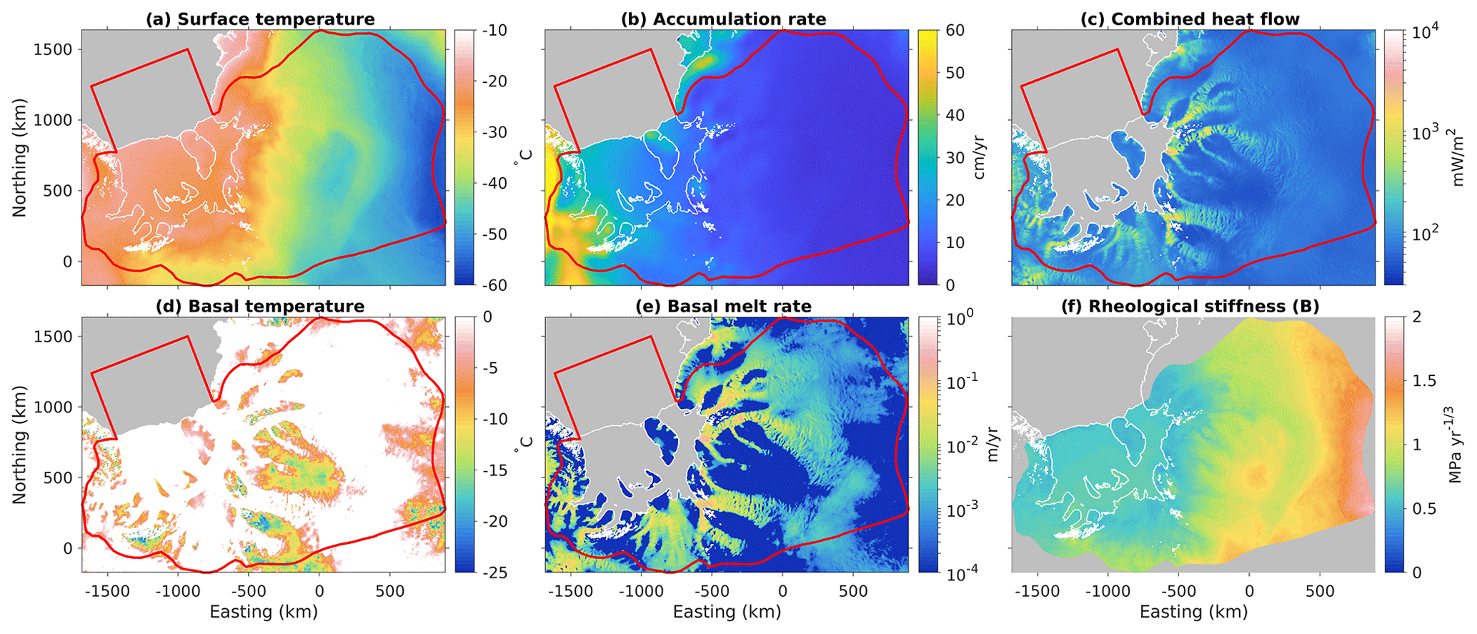
Figure A1Thermal forcing and ice rheology. Top row (a–c) shows the boundary conditions (surface temperature, surface accumulation rate, and basal heat flow) used to force the 1D thermal model. Bottom row (d–f) shows model output: basal temperature, basal melt rate, and column-average rheological stiffness parameter. Basal temperature has been corrected for the pressure dependence of the melting point.
The resulting thermal structure is shown in Fig. A1d–f. Basal temperature is at the pressure-dependent melting point in most of the domain, including almost all of the fast-flowing regions. Basal melt rate varies between about 0.1 and 1 m a−1, with values above 1 cm a−1 being exclusively due to high rates of shear heating. We use the thermal model to compute a vertically variable rheology stiffness parameter B based on Cuffey and Paterson (2010, p. 75), which we then average vertically to produce the parameter needed by the SSA model (Fig. A1f). varies spatially by about a factor of 4 between its largest and smallest values, with most of the spatial structure attributable to gradients in surface temperature (Fig. A1; cf. plots (a) and (f)).
A2 Numerical mesh
For our numerical mesh, we use an unstructured triangular mesh in the map-view plane, constructed using the bidimensional anisotropic mesh generator (BAMG, Hecht, 2006). As is common in finite-element glaciological modeling, we want to refine our mesh in dynamically important regions, such as fast-flowing ice streams and outlet glaciers, or the grounding line and calving front. However, we also wish to investigate the influence of mesh resolution on our inversion results, which means that we need to create multiple meshes with different resolution but a similar spatial pattern of refinement. We do this by constructing a common control field for all of our meshes and then systematically varying parameters that control how the mesh is constructed from that control field.
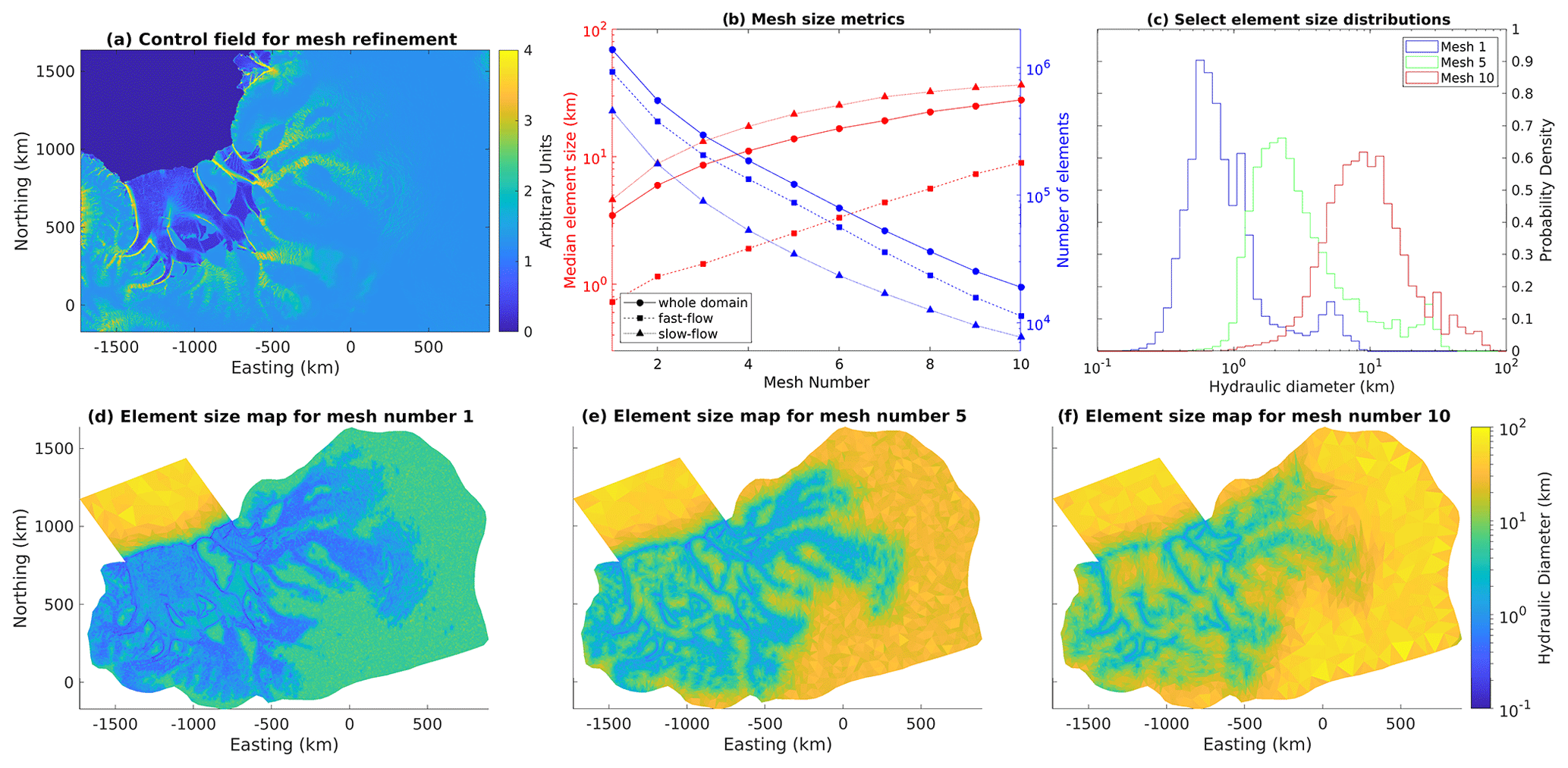
Figure A2Element size analysis for our series of meshes. (a) The common control field used to refine all of the meshes. (b) Analysis of median element size and number of elements for each mesh in the series. Separate plots are shown for the entire grounded domain, as well as the grounded domain split into fast-flowing and slow-flowing regions. We define “fast flow” as , with a smooth weighting function between 7.5 and 30 m a−1. (c) Selected histograms of element size within the grounded fast-flow domain. (d–f) Maps of element size for the same selected meshes. Note that median size in (b) and probability density in (c) are defined with respect to domain area, not element number; i.e., a median size of X means that 50 % of the domain area is covered by elements smaller than X, not that 50 % of the elements themselves are smaller than X.
We construct a control field on a 1 km regular grid using the logarithm of potential energy dissipation (the dot product of driving stress and ice velocity) in the grounded domain, the logarithm of strain-rate magnitude in the floating domain, and adding a constant multiple of the mask in order to produce discontinuities at the grounding line and calving front (Fig. A2a). We use BAMG to iteratively refine the mesh so as to minimize interpolation errors in the control field; thus, the mesh will be refined in areas where the control field has sharp curvature and the mesh will be unrefined in areas where the control field is smooth. We generate 10 meshes using values of the BAMG parameters err, the acceptable level of interpolation error, ranging linearly from 0.01 to 0.1; values of hmin, the minimum edge length, ranging from 0.1 to 1.0 km; and values of hmax, the maximum edge length, ranging from 10 km to 100 km.
The resulting meshes are summarized in Fig. A2. We use the hydraulic diameter (4 × area/perimeter) to be a representative linear size metric for our mesh elements, with the factor of 4 chosen such that the hydraulic diameter of a circle would be equal to the regular diameter. All of our meshes share a common spatial pattern of refinement (Fig. A2d–f) that they inherited from the control field (Fig. A2a). We analyze fast-flowing and slow-flowing regions separately, using a smooth weighting function generated by applying a cosine taper to the logarithm of velocity. The 50 % cutoff of the weighting function was 15 m a−1, with 0 %–100 % limits at 7.5 and 30 m a−1. These velocity thresholds are relatively low, but we choose them as approximate values roughly separating the beginning of streaming flow from slow flow. Element size in both the fast- and slow-flowing regions varies smoothly between different meshes, but element size in the fast-flow region is consistently ∼7 times smaller than in the slow-flow region, and the mesher places about of the grounded elements within the fast-flowing region (Fig. A2b), despite the fact that the fast-flowing region is only about of the grounded area. An analysis of histograms of element size in the fast-flowing region reveals that our meshing procedure produces similar statistical distributions of element size for each mesh, simply shifted towards larger or smaller size (Fig. A2c). Although BAMG is an anisotropic mesh generator, in practice most of our mesh elements are fairly close to equilateral triangles, with the overwhelming majority of our grounded domain area being covered by elements having an anisotropy ratio less than 2 (Fig. A3).
Once the meshes were generated, we interpolated all relevant fields (e.g., geometry, velocity) onto each mesh using a multi-wavelength technique, described below (Sect. A3). We reordered the mask into a series that behaves in an ice dynamically reasonable manner under smoothing and interpolation operations prior to interpolation (Sect. A4).
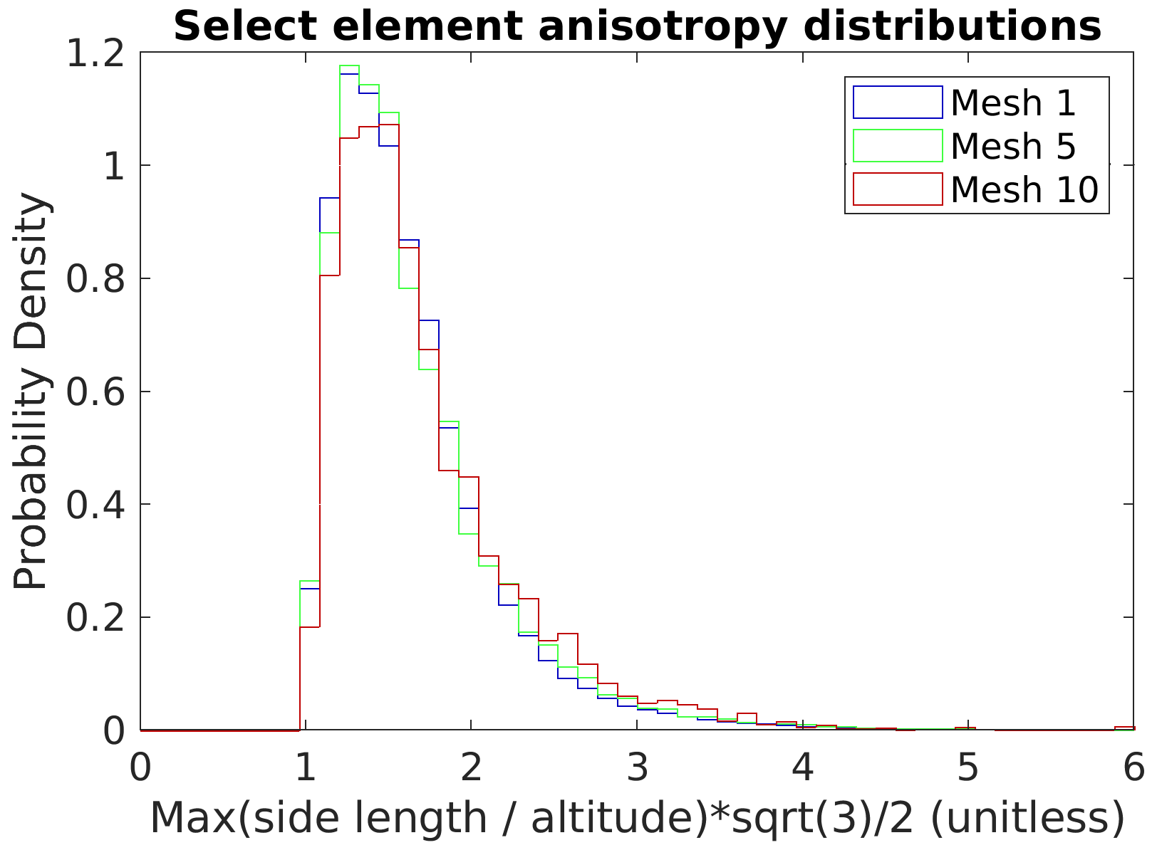
Figure A3Element anisotropy for select meshes. This figure shows the distribution of element anisotropy for the same select three meshes shown in Fig. A2. Element anisotropy is measured as the maximum ratio of side length to altitude, scaled such that an equilateral triangle has a value of 1. As in Fig. A2c, probability density has been scaled by element area. Values shown are computed for the whole grounded domain.
A3 Multi-wavelength method for data interpolation
Our model setup requires that various data products be interpolated from their native regular square grids onto our unstructured triangular meshes. For instance, our ice geometry data are taken from BedMachine Antarctica Version 2 (Morlighem, 2020; Morlighem et al., 2020), which has a native grid resolution of 500 m, although the underlying radar data used to generate the gridded product have a highly variable flight line spacing that is usually at least several kilometers. Meanwhile, our model meshes have spatially variable resolution: for instance, mesh no. 1 has a median element size less than 1 km in the fast-flow region but an element size of 10 km in the slow-flow region. A simple naive interpolation, such as bilinear or spline, would therefore produce aliasing in slow-flowing areas with variable geometry, such as the Gamburtsev Subglacial Mountains. In such an area, mesh nodes that happened to fall in subglacial valleys would be assigned a very large ice thickness, while mesh nodes that happened to fall on subglacial peaks would be assigned a very small ice thickness, producing noisy and erroneous large-scale gradients in thickness. In reality, it would be better to assign each mesh node an intermediate value of ice thickness that was representative of a larger area comparable to the local element size. However, a simple naive interpolation from the original grid would still be appropriate in areas where the model mesh is fine; where element size is small, we would like to take advantage of the full information content of the gridded product without losing any information to smoothing.
Thus, we developed a multi-wavelength smoothing procedure for interpolating gridded data products onto our model mesh. The objective of this procedure is to ensure that each mesh node receives an interpolated value that is representative of the average of the original data grid over an area comparable to the local element size. Where mesh resolution is fine, mesh nodes receive values interpolated from a high-resolution grid, and where mesh resolution is course, the nodes receive values interpolated from a highly smoothed grid. The procedure is as follows:
-
First, we generate multiple copies of the original grid smoothed at a range of wavelengths. Starting from the original full-resolution grid, each subsequent grid is generated by twice smoothing the previous grid with a 3×3 box filter and then decimating by a factor of 2 in both dimensions. Thus, the spatial resolution of each subsequent grid is a factor of 2 coarser than the previous grid (and the space used in memory is reduced by a factor of 4). This process of smoothing and downsampling is continued until we reach a resolution comparable to the coarsest elements in the mesh.
-
Next, we need to calculate a characteristic local element size for each mesh vertex. This is done by first computing the hydraulic radius for each element (half the hydraulic diameter, or 2 × area/perimeter) and then averaging hydraulic radius from the elements to the vertices.
-
Finally, we can interpolate the data from our grids to the mesh vertices. Each vertex is assigned to the first grid with a resolution coarser than its hydraulic radius. We loop through the grids, and for each grid, we perform a simple bilinear interpolation from that grid onto the vertices that were assigned to it.
This procedure produces an interpolated product that both avoids aliasing in coarse-resolution regions of the mesh and preserves high-resolution information where the mesh is fine. Additionally, while this method is not exactly conservative, it is approximately so: integrated ice volume within our domain computed on the mesh was within a factor of 10−4 of the value computed on the grid. We applied this method for all gridded data products that needed to be interpolated onto our meshes, including both components of the velocity observations. We applied a reordering to the BedMachine mask to ensure that it would behave logically under smoothing and interpolation operations, as described below. A MATLAB function for performing this method (MultiWavelengthInterpolator.m) is available on our Zenodo code and data release page.
A4 Mask reordering
The smoothing and interpolation of mask values can be especially tricky, as there is not always a straightforward interpretation of intermediate values between the original integer classes. For instance, BedMachine has a mask variable with the following five values: 0 – open ocean, 1 – exposed rock, 2 – grounded ice sheet, 3 – floating ice shelf, and 4 – Lake Vostok. Lake Vostok is not located within our domain, leaving us with four remaining integer mask values1. Often, modelers will interpolate mask values using nearest neighbor interpolation, thus ensuring that they only get integer results and they do not need to do the hard work of interpreting intermediate values. However, nearest neighbor interpolation will not necessarily produce values that are spatially representative. For instance, if a single mesh vertex happens to find the lone nunatak in an otherwise ice-covered region, then the apparent area of that nunatak in the model mesh would be much greater than reality. Our multi-wavelength interpolation procedure, described above, can produce values that are spatially representative, but these values will not necessarily be integer-valued, and we thus need a way to interpret intermediate values of the interpolated mask.
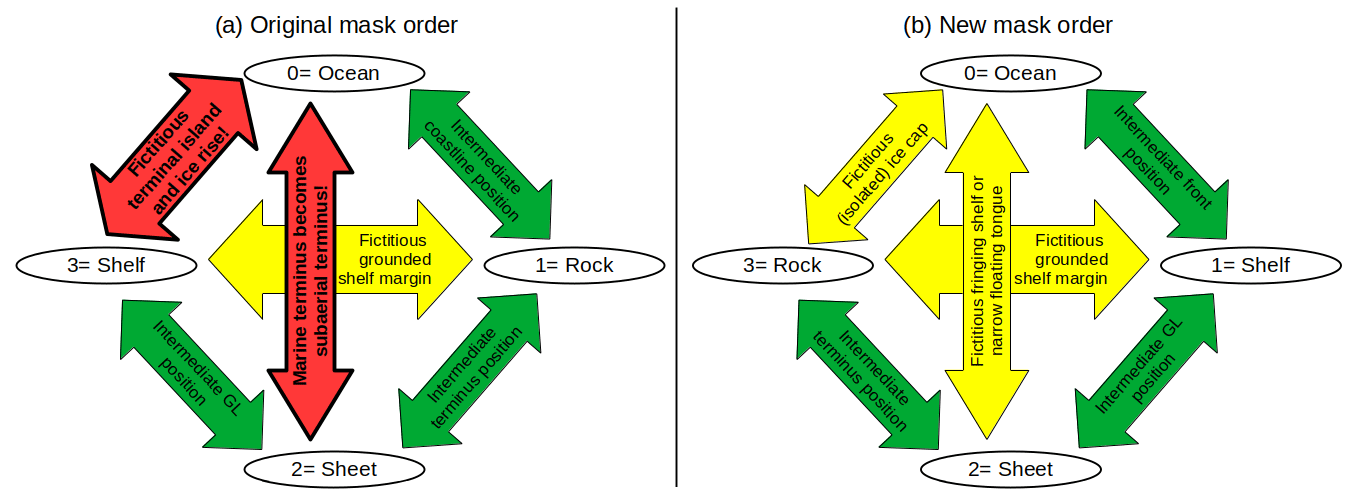
Figure A4Flowchart showing all combinations of intermediate values for both the original (a) and the new (b) mask order. Combinations are colored green when intermediate values do not change the ice sheet configuration and can be simply interpreted as area fractions or intermediate positions, yellow when intermediate values produce new ice sheet configurations that do not have a significant influence on the force balance or overall dynamics of the ice sheet, and red when intermediate values they produce new ice sheet configurations that are extremely disruptive of the overall force balance or dynamics.
Unfortunately, the original BedMachine mask order does not always behave in an ice dynamically reasonable manner under smoothing and interpolation operations. We consider behavior to be most “reasonable” when intermediate fractional mask values can be easily interpreted as either area fractions of the respective regions or as an intermediate boundary position, for instance if an interpolated mask value in between grounded ice sheet and floating ice shelf can be simply interpreted as grounded area fraction. We consider behavior to be moderately unreasonable when intermediate values change the configuration but in a way that does not produce big disturbances in the force balance or overall dynamics, for instance if interpolation between a grounded ice sheet and the open ocean produces a narrow floating shelf at the terminus that provides no appreciable buttressing. And we consider behavior to be egregiously unreasonable if intermediate values change the ice sheet configuration in a way that produces a major change in force balance or dynamics, for instance if interpolation between floating ice shelf and open ocean produces a ring of grounded ice rises at the terminus.
The original mask order produces two egregiously unreasonable intermediate states (Fig. A4a): interpolation between open ocean (0) and a floating ice shelf (3) produces fictitious rock islands (1) and grounded ice rises (2) at the terminus of the shelf, thus drastically increasing the amount of buttressing, and interpolation between grounded ice sheet (2) and open ocean (0) creates exposed rock (1), thus transforming a tidewater marine terminus into a grounded terminus. Additionally, interpolation between exposed rock (1) and a floating ice shelf (3) produces a thin region of grounded ice (2) around the fringe of the ice shelf, but we consider this to be only a moderately unreasonable change, since an ice shelf in contact with the rock walls of an embayment ought to be already experiencing buttressing.
However, the two egregiously unreasonable intermediate states in the original mask order can be eliminated by a simple reordering of the mask values. The only change required is that the numbers representing exposed rock and floating ice shelf are swapped, such that the mask now goes as follows: 0 – open ocean, 1 – floating ice shelf, 2 – grounded ice sheet, and 3 – exposed rock. Under this order, no intermediate values are more than moderately unreasonable (Fig. A4b) and none have a disruptive influence on the ice sheet force balance. Under this order, intermediate values at the ice shelf front (contact between 0 and 1) are easily interpreted as area fraction of ice or intermediate front position. Interpolation at a grounded terminus (contact between 0 and 2) will produce a small fictitious floating tongue (1), but this tongue should be unbuttressed and therefore will have little effect on the overall force balance. Interpolation between a floating shelf (1) and exposed rock (3) will have the same effect as before; the only new unreasonable configuration will be interpolation between exposed rock (3) and open ocean (0), which should produce a brand-new ice cap (2) and small floating shelf (1). However, this new ice cap will be isolated from the rest of the ice sheet (because it occurs at the contact between rock and ocean) and therefore will have no influence on the force balance of the true ice sheet.
This point is admittedly tangential to the main topic of our paper, but we find it striking that a simple reordering of the mask can produce behavior under smoothing and interpolation operations that is far more reasonable from an ice dynamic perspective than the original mask order. After reordering of the mask as described here, we used the same multi-wavelength interpolation procedure described above to interpolate the reordered mask onto the model mesh. Finally, we removed areas with an ice thickness less than 10 m from the active region of our inversion by setting those areas to either exposed rock or open ocean, depending on their bed elevation.
A5 Curve-fitting for L-curve analysis
For our L-curve analysis, we sample the range with 25 logarithmically spaced samples, resulting in 4 repeating samples per decade . For each sample, we run the inverse model to convergence using M1QN3 and record Jobs and Jreg. We used a stopping tolerance of 10−5 for the ratio of the gradient magnitude to the initial gradient magnitude, although we had to tighten this tolerance to 10−6 and 10−7 in order to produce monotonic L-curves for our inversions with m=3 and m=5, respectively. An example of the result is shown by the black dots in Fig. 3a.
Before selecting the optimal λ value, we next construct a smoothed tradeoff curve in (ln (Jreg), ln (Jobs)) space based on our 25 individual model results. Constructing a smoothed curve is necessary because we identify the corner of the L-curve by computing the curvature of our cost function components, and taking the second derivative tends to amplify noise. Our smoothed curve is a parametric function of λ with two components: Jr,c and Jo,c. To make the smoothed tradeoff curve, we first subsampled our 25 individual model results onto 1000 logarithmically spaced λ subsamples. We then tested 50 different smoothing wavelengths, ranging from a minimum of half the separation of the original model points to a maximum of ln (100). Note that all smoothing was performed in ln (λ) space.
The selection of the optimal smoothing wavelength in ln (λ) space can be regarded as a sort of meta-regularization: increased smoothing results in a worse fit between the tradeoff curve and the original model points, but reduced smoothing increases the random fluctuations in the curvature of the tradeoff curve. We would like to select a smoothing wavelength that balances these concerns. Thus, for each smoothing wavelength we computed the variance due to curvature of the smoothed curve and the variance due to scatter of the original model points about the smoothed curve. These variances are
where Vs and Vc are the scatter and curvature variances of the curves, (Jobs,Jreg) are the cost function components from the N individual inverse models, and are the cost function components from the smoothed tradeoff curve. As in our original analysis, both Vs and Vc need to be normalized before they can be combined; we simply normalized each by their respective maximum values and then added them together and selected the wavelength that minimized the combined variance.
Once we have a smoothed tradeoff curve, we computed the total logarithmic curvature from (Fig. 3d). The location of maximum curvature represents the sharpest corner in the L-curve and the best-value λ. We also record where the total curvature drops to of its maximum value, in order to bracket the full range of the corner. Thus, we have three λ values: minimum acceptable, best, and maximum acceptable. The logarithmic uncertainty in these three λ values is given by the smoothing wavelength chosen above. The value of of maximum curvature that we used to define λmin and λmax is an arbitrary heuristic, and the arbitrariness of this choice introduces an additional degree of uncertainty into our estimate of those two λ values. For most of our L-curves, we found that the drop-off in total curvature below λbest was quite steep (Fig. 3d), so the choice of as our threshold value should have little influence on our estimate of λmin. However, the drop-off in total curvature above λbest was more gradual, so our estimated λmax values should be regarded as more uncertain.
B1 Coefficient conversion
Despite being a poor representation of reality (Sect. 5.1), linear Weertman sliding has the advantage of being the sliding law that is the easiest to implement numerically. Some ice sheet models, such as Elmer/Ice (Gagliardini et al., 2013), only contain the ability to invert for a linear Weertman drag coefficient; if users of that model want to use a different sliding law constrained by observations, they must first perform an inversion for the linear Weertman coefficient and then convert that coefficient to the alternate sliding law. Thus, we think it is a useful experiment to test whether such a conversion does a good job of reproducing the inversion results and L-curve generated by the nonlinear sliding law.
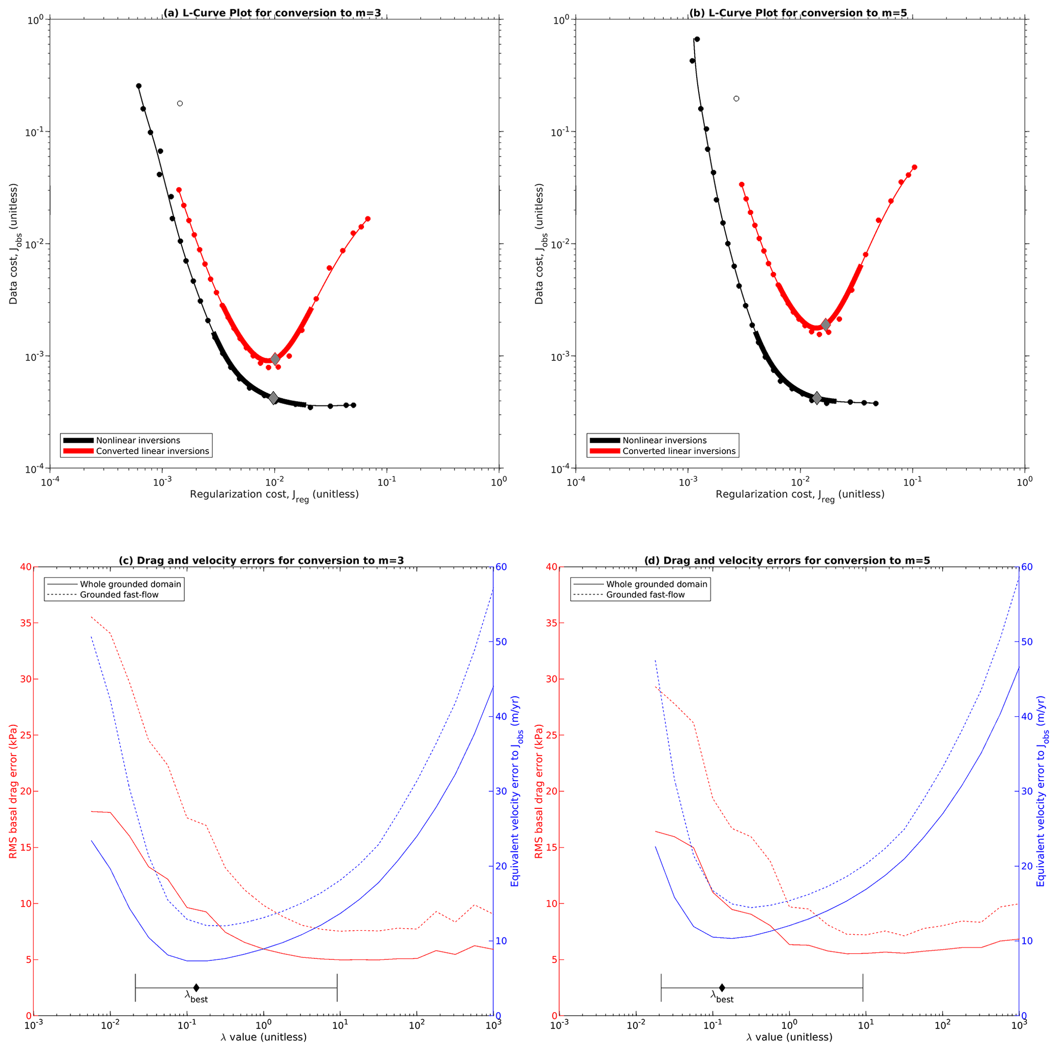
Figure B1Effectiveness of converting the slip coefficient from a linear sliding law to a nonlinear one. (a) Converted linear L-curve compared to the L-curve computed for m=3. Display as in Figs. 3, 8, 9, and 11. For the converted linear L-curve, the same smoothing wavelength has been used to construct the smoothed L-curve as was used for the original linear L-curve, and the indicated λbest value and corner region are also those determined from the original linear L-curve. (b) As (a) but for m=5. (c) Plot of errors in basal drag and ice velocity for the linear results converted to m=3. Drag error has been computed by matching converted linear models with nonlinear models according to . Velocity error is computed with respect to the observations. (d) As (c) but for m=5.
We converted our linear Weertman drag coefficient to a nonlinear sliding law using
where Cm is the converted coefficient for the new exponent, and CW is the coefficient for linear Weertman sliding. We performed this conversion separately for all 25 inversions in our linear Weertman L-curve on our highest resolution mesh. We tested the conversion from m=1 to both m=3 and m=5. For each converted coefficient, we ran a single stress balance solve to get a new velocity field, from which we computed Jobs. We also computed Jreg for the converted coefficient using the same scale estimates we used for the corresponding nonlinear inversions. Thus, we are able to directly compare L-curve shape between the converted linear inversions and the fully nonlinear inversions.
As can be seen in Fig. B1a and b, the converted linear L-curve is nonmonotonic for both m=3 and m=5. For large λ, the slope of the converted linear L-curve roughly follows the large-λ limb of the nonlinear L-curve, although its position is shifted towards higher Jreg values (and we know this shift is meaningful because we used the same scale estimate for both L-curves). However, below λbest, the converted linear L-curve turns around sharply. Jobs stops declining and begins rising again, eventually attaining values roughly as high as those in the large-λ limb. This sharp increase in velocity error for λ<λbest is consistent regardless of whether the error is computed in the whole grounded domain or in the fast-flow region alone (Fig. B1c, d). We also attempted to compare basal drag between the converted linear inversions and the nonlinear inversions. Such a comparison is more ambiguous because the nonlinear L-curves have a different value of λbest, so we chose to match models between the nonlinear L-curves and the converted linear L-curves according to . Doing so reveals that the discrepancy in basal drag between the nonlinear results and the converted linear results also increases sharply for small λ (Fig. B1c, d).
Thus, these results demonstrate that L-curve analysis can be a valuable tool even for modelers who intend to convert their coefficient from linear Weertman to a new sliding law. Conversion of the coefficient without performing an L-curve analysis first may produce unreliable results, especially for λ<λbest. However, for λ≈λbest the conversion is likely to give results that, while not quite as good as those obtained from a nonlinear inversion directly, are still broadly reasonable. Our recommendation for modelers performing coefficient conversion is that they should first construct an L-curve for their linear Weertman inversion and then convert the coefficient obtained for λbest.
Inversion scripts, inverse model results, L-curve summaries, and our best combined drag estimate are available at https://doi.org/10.5281/zenodo.7798650 (Wolovick et al., 2023). The best combined drag estimate is presented interpolated onto a regular grid in NetCDF format for ease of use. The ice flow model ISSM is open source and freely available at https://issm.jpl.nasa.gov/ (Larour et al., 2012). Here ISSM version 4.18 was used.
MJW wrote inversion scripts, devised experimental design, made figures, and prepared the manuscript text. TK ran the CUAS hydrology model. AH and MR acquired funding and supervised the work. MR installed and maintained the ISSM installation on AWI's HPC system. All authors contributed to the revision and improvements of the manuscript as well as discussions about ideas and conclusions.
The contact author has declared that none of the authors has any competing interests.
Publisher's note: Copernicus Publications remains neutral with regard to jurisdictional claims made in the text, published maps, institutional affiliations, or any other geographical representation in this paper. While Copernicus Publications makes every effort to include appropriate place names, the final responsibility lies with the authors.
We thank the two anonymous reviewers for their thorough and rigorous comments on our manuscript. Additionally, we thank Christian Schoof for correcting a mistake in Eq. (1).
This research has been supported by the Alfred-Wegener-Institut Helmholtz-Zentrum für Polar- und Meeresforschung under the INSPIRESII project FRISio.
The article processing charges for this open-access publication were covered by the Alfred-Wegener-Institut Helmholtz-Zentrum für Polar- und Meeresforschung.
This paper was edited by Alexander Robinson and reviewed by two anonymous referees.
Andrews, L. C., Catania, G. A., Hoffman, M. J., Gulley, J. D., Luthi, M. P., Ryser, C., Hawley, R. L., and Neumann, T. A.: Direct observations of evolving subglacial drainage beneath the Greenland Ice Sheet, Nature, 514, 80–83, https://doi.org/10.1038/nature13796, 2014. a
Arthern, R. J. and Gudmundsson, G. H.: Initialization of ice-sheet forecasts viewed as an inverse Robin problem, J. Glaciol., 56, 527–533, https://doi.org/10.3189/002214310792447699, 2010. a, b, c
Arthern, R. J., Winebrenner, D. P., and Vaughan, D. G.: Antarctic snow accumulation mapped using polarization of 4.3-cm wavelength microwave emission, J. Geophys. Res.-Atmos., 111, D06107, https://doi.org/10.1029/2004JD005667, 2006. a
Arthern, R. J., Hindmarsh, R. C. A., and Williams, C. R.: Flow speed within the Antarctic ice sheet and its controls inferred from satellite observations, J. Geophys. Res.-Earth, 120, 1171–1188, https://doi.org/10.1002/2014JF003239, 2015. a
Bamber, J. L., Layberry, R. L., and Gogineni, S. P.: A new ice thickness and bed data set for the Greenland ice sheet: 1. Measurement, data reduction, and errors, J. Geophys. Res.-Atmos., 106, 33773–33780, https://doi.org/10.1029/2001JD900054, 2001. a
Bamber, J. L., Gomez-Dans, J. L., and Griggs, J. A.: A new 1 km digital elevation model of the Antarctic derived from combined satellite radar and laser data – Part 1: Data and methods, The Cryosphere, 3, 101–111, https://doi.org/10.5194/tc-3-101-2009, 2009. a
Bamber, J. L., Griggs, J. A., Hurkmans, R. T. W. L., Dowdeswell, J. A., Gogineni, S. P., Howat, I., Mouginot, J., Paden, J., Palmer, S., Rignot, E., and Steinhage, D.: A new bed elevation dataset for Greenland, The Cryosphere, 7, 499–510, https://doi.org/10.5194/tc-7-499-2013, 2013. a
Barnes, J. M. and Gudmundsson, G. H.: The predictive power of ice sheet models and the regional sensitivity of ice loss to basal sliding parameterisations: a case study of Pine Island and Thwaites glaciers, West Antarctica, The Cryosphere, 16, 4291–4304, https://doi.org/10.5194/tc-16-4291-2022, 2022. a
Beyer, S., Kleiner, T., Aizinger, V., Rückamp, M., and Humbert, A.: A confined–unconfined aquifer model for subglacial hydrology and its application to the Northeast Greenland Ice Stream, The Cryosphere, 12, 3931–3947, https://doi.org/10.5194/tc-12-3931-2018, 2018. a, b
Blatter, H.: Velocity and stress fields in grounded glaciers – a simple algorithm for including deviatoric stress gradients, J. Glaciol., 41, 333–344, 1995. a
Brondex, J., Gillet-Chaulet, F., and Gagliardini, O.: Sensitivity of centennial mass loss projections of the Amundsen basin to the friction law, The Cryosphere, 13, 177–195, https://doi.org/10.5194/tc-13-177-2019, 2019. a
Budd, W. F., Keage, P. L., and Blundy, N. A.: Empirical Studies of Ice Sliding, J. Glaciol., 23, 157–170, https://doi.org/10.1017/S0022143000029804, 1979. a
Comiso, J. C.: Variability and trends in Antarctic surface temperatures from in situ and satellite infrared measurements, J. Climate, 13, 1674–1696, https://doi.org/10.1175/1520-0442(2000)013<1674:VATIAS>2.0.CO;2, 2000. a
Cuffey, K. and Paterson, W.: The Physics of Glaciers, Butterworth-Heineman/Elsevier, Burlington, MA, 4th Edn., ISBN 978-0-12-369461-4, 2010. a, b
Fahnestock, M., Scambos, T., Moon, T., Gardner, A., Haran, T., and Klinger, M.: Rapid large-area mapping of ice flow using Landsat 8, Remote Sens. Environ., 185, 84–94, https://doi.org/10.1016/j.rse.2015.11.023, 2016. a
Fischler, Y., Kleiner, T., Bischof, C., Schmiedel, J., Sayag, R., Emunds, R., Oestreich, L. F., and Humbert, A.: A parallel implementation of the confined–unconfined aquifer system model for subglacial hydrology: design, verification, and performance analysis (CUAS-MPI v0.1.0), Geosci. Model Dev., 16, 5305–5322, https://doi.org/10.5194/gmd-16-5305-2023, 2023. a, b
Fretwell, P., Pritchard, H. D., Vaughan, D. G., Bamber, J. L., Barrand, N. E., Bell, R., Bianchi, C., Bingham, R. G., Blankenship, D. D., Casassa, G., Catania, G., Callens, D., Conway, H., Cook, A. J., Corr, H. F. J., Damaske, D., Damm, V., Ferraccioli, F., Forsberg, R., Fujita, S., Gim, Y., Gogineni, P., Griggs, J. A., Hindmarsh, R. C. A., Holmlund, P., Holt, J. W., Jacobel, R. W., Jenkins, A., Jokat, W., Jordan, T., King, E. C., Kohler, J., Krabill, W., Riger-Kusk, M., Langley, K. A., Leitchenkov, G., Leuschen, C., Luyendyk, B. P., Matsuoka, K., Mouginot, J., Nitsche, F. O., Nogi, Y., Nost, O. A., Popov, S. V., Rignot, E., Rippin, D. M., Rivera, A., Roberts, J., Ross, N., Siegert, M. J., Smith, A. M., Steinhage, D., Studinger, M., Sun, B., Tinto, B. K., Welch, B. C., Wilson, D., Young, D. A., Xiangbin, C., and Zirizzotti, A.: Bedmap2: improved ice bed, surface and thickness datasets for Antarctica, The Cryosphere, 7, 375–393, https://doi.org/10.5194/tc-7-375-2013, 2013. a
Gagliardini, O., Cohen, D., Råback, P., and Zwinger, T.: Finite-element modeling of subglacial cavities and related friction law, J. Geophys. Re.-Earth, 112, F02027, https://doi.org/10.1029/2006JF000576, 2007. a, b, c
Gagliardini, O., Zwinger, T., Gillet-Chaulet, F., Durand, G., Favier, L., de Fleurian, B., Greve, R., Malinen, M., Martín, C., Råback, P., Ruokolainen, J., Sacchettini, M., Schäfer, M., Seddik, H., and Thies, J.: Capabilities and performance of Elmer/Ice, a new-generation ice sheet model, Geosci. Model Dev., 6, 1299–1318, https://doi.org/10.5194/gmd-6-1299-2013, 2013. a, b
Gillet-Chaulet, F., Gagliardini, O., Seddik, H., Nodet, M., Durand, G., Ritz, C., Zwinger, T., Greve, R., and Vaughan, D. G.: Greenland ice sheet contribution to sea-level rise from a new-generation ice-sheet model, The Cryosphere, 6, 1561–1576, https://doi.org/10.5194/tc-6-1561-2012, 2012. a, b, c, d
Gillet-Chaulet, F., Durand, G., Gagliardini, O., Mosbeux, C., Mouginot, J., Rémy, F., and Ritz, C.: Assimilation of surface velocities acquired between 1996 and 2010 to constrain the form of the basal friction law under Pine Island Glacier, Geophys. Res. Lett., 43, 10311–10321, https://doi.org/10.1002/2016GL069937, 2016. a, b, c
Glen, J. W.: Rate of flow of polycrystalline ice, Nature, 172, 721–722, https://doi.org/10.1038/172721a0, 1953. a
Goldberg, D. N.: A variationally derived, depth-integrated approximation to a higher-order glaciological flow model, J. Glaciol., 57, 157–170, 2011. a
Gudmundsson, G. H.: Transmission of basal variability to a glacier surface, J. Geophys. Res.-Sol. Ea., 108, 2253, https://doi.org/10.1029/2002JB002107, 2003. a
Gudmundsson, G. H.: Ice-stream response to ocean tides and the form of the basal sliding law, The Cryosphere, 5, 259–270, https://doi.org/10.5194/tc-5-259-2011, 2011. a
Habermann, M., Maxwell, D., and Truffer, M.: Reconstruction of basal properties in ice sheets using iterative inverse methods, J. Glaciol., 58, 795–808, https://doi.org/10.3189/2012jog11j168, 2012. a, b
Habermann, M., Truffer, M., and Maxwell, D.: Changing basal conditions during the speed-up of Jakobshavn Isbræ, Greenland, The Cryosphere, 7, 1679–1692, https://doi.org/10.5194/tc-7-1679-2013, 2013. a, b, c, d, e, f
Hansen, P. C.: Analysis of Discrete Ill-Posed Problems by Means of the L-Curve, SIAM Revi., 34, 561–580, https://doi.org/10.1137/1034115, 1992. a
Hansen, P. C. and O'Leary, D. P.: The Use of the L-Curve in the Regularization of Discrete Ill-Posed Problems, SIAM J. Sci. Comput., 14, 1487–1503, https://doi.org/10.1137/0914086, 1993. a, b, c, d, e
Hecht, F.: BAMG: Bidimensional Anisotropic Mesh Generator, Tech. rep., FreeFem++, https://www.ljll.math.upmc.fr/hecht/ftp/bamg (last access: 11 April 2023), 2006. a
Hofstede, C., Beyer, S., Corr, H., Eisen, O., Hattermann, T., Helm, V., Neckel, N., Smith, E. C., Steinhage, D., Zeising, O., and Humbert, A.: Evidence for a grounding line fan at the onset of a basal channel under the ice shelf of Support Force Glacier, Antarctica, revealed by reflection seismics, The Cryosphere, 15, 1517–1535, https://doi.org/10.5194/tc-15-1517-2021, 2021. a
Iken, A.: The effect of the subglacial water pressure on the sliding velocity of a glacier in an idealized numerical model, J. Glaciol., 27, 407–421, 1981. a, b
Joughin, I., MacAyeal, D., and Tulaczyk, S.: Basal shear stress of the Ross ice streams from control method inversions, J. Geophys. Res.-Sol. Ea., 109, B09405, https://doi.org/10.1029/2003JB002960, 2004. a, b, c, d
Joughin, I., Bamber, J. L., Scambos, T., Tulaczyk, S., Fahnestock, M., and MacAyeal, D. R.: Integrating satellite observations with modelling: basal shear stress of the Filcher-Ronne ice streams, Antarctica, Philos. T. Roy. Soc. A-Math., 364, 1795–1814, https://doi.org/10.1098/rsta.2006.1799, 2006. a, b, c, d
Joughin, I., Tulaczyk, S., Bamber, J. L., Blankenship, D., Holt, J. W., Scambos, T., and Vaughan, D. G.: Basal conditions for Pine Island and Thwaites Glaciers, West Antarctica, determined using satellite and airborne data, J. Glaciol., 55, 245–257, https://doi.org/10.3189/002214309788608705, 2009. a, b, c
Joughin, I., Smith, B. E., and Holland, D. M.: Sensitivity of 21st century sea level to ocean-induced thinning of Pine Island Glacier, Antarctica, Geophys. Res. Lett., 37, L20502, https://doi.org/10.1029/2010GL044819, 2010a. a, b
Joughin, I., Smith, B. E., Howat, I. M., Scambos, T., and Moon, T.: Greenland flow variability from ice-sheet-wide velocity mapping, J. Glaciol., 56, 415–430, https://doi.org/10.3189/002214310792447734, 2010b. a
Kamb, B.: Rheological nonlinearity and flow instability in the deforming bed mechanism of ice stream motion, J. Geophys. Res.-Sol. Ea., 96, 16585–16595, https://doi.org/10.1029/91JB00946, 1991. a
Kamb, B., Raymond, C. F., Harrison, W. D., Engelhardt, H., Echelmeyer, K. A., Humphrey, N., Brugman, M. M., and Pfeffer, T.: Glacier Surge Mechanism: 1982-1983 Surge of Variegated Glacier, Alaska, Science, 227, 469–479, https://doi.org/10.1126/science.227.4686.469, 1985. a
Kazmierczak, E., Sun, S., Coulon, V., and Pattyn, F.: Subglacial hydrology modulates basal sliding response of the Antarctic ice sheet to climate forcing, The Cryosphere, 16, 4537–4552, https://doi.org/10.5194/tc-16-4537-2022, 2022. a
Larour, E., Rignot, E., Joughin, I., and Aubry, D.: Rheology of the Ronne Ice Shelf, Antarctica, inferred from satellite radar interferometry data using an inverse control method, Geophys. Res. Lett., 32, L05503, https://doi.org/10.1029/2004GL021693, 2005. a
Larour, E., Seroussi, H., Morlighem, M., and Rignot, E.: Continental scale, high order, high spatial resolution, ice sheet modeling using the Ice Sheet System Model (ISSM), J. Geophys. Res.-Earth, 117, F01022, https://doi.org/10.1029/2011JF002140, 2012 (code available at: https://issm.jpl.nasa.gov/, last access: 6 May 2021). a, b
Larour, E., Utke, J., Csatho, B., Schenk, A., Seroussi, H., Morlighem, M., Rignot, E., Schlegel, N., and Khazendar, A.: Inferred basal friction and surface mass balance of the Northeast Greenland Ice Stream using data assimilation of ICESat (Ice Cloud and land Elevation Satellite) surface altimetry and ISSM (Ice Sheet System Model), The Cryosphere, 8, 2335–2351, https://doi.org/10.5194/tc-8-2335-2014, 2014. a
Le Brocq, A. M., Payne, A. J., and Vieli, A.: An improved Antarctic dataset for high resolution numerical ice sheet models (ALBMAP v1), Earth Syst. Sci. Data, 2, 247–260, https://doi.org/10.5194/essd-2-247-2010, 2010a. a
Le Brocq, A. M. L., Payne, A. J., and Vieli, A.: An improved Antarctic dataset for high resolution numerical ice sheet models (ALBMAP v1), PANGEA [data set], https://doi.org/10.1594/PANGAEA.734145, 2010b. a
Lythe, M. B. and Vaughan, D. G.: BEDMAP: A new ice thickness and subglacial topographic model of Antarctica, J. Geophys. Res.-Sol. Ea., 106, 11335–11351, https://doi.org/10.1029/2000JB900449, 2001. a
MacAyeal, D.: Large-scale ice flow over a viscous basal sediment: Theory and application to ice stream B, Antarctica, J. Geophys. Res.-Sol. Ea., 94, 4071–4087, https://doi.org/10.1029/JB094iB04p04071, 1989. a
MacAyeal, D.: A tutorial on the use of control methods in ice-sheet modeling, J. Glaciol., 39, 91–98, 1993. a, b, c, d, e, f
Martin, N. and Monnier, J.: Adjoint accuracy for the full Stokes ice flow model: limits to the transmission of basal friction variability to the surface, The Cryosphere, 8, 721–741, https://doi.org/10.5194/tc-8-721-2014, 2014. a
Martos, Y. M.: Antarctic geothermal heat flux distribution and estimated Curie Depths, PANGAEA [data set], https://doi.org/10.1594/PANGAEA.882503, 2017. a
Martos, Y. M., Catalán, M., Jordan, T. A., Golynsky, A., Golynsky, D., Eagles, G., and Vaughan, D. G.: Heat Flux Distribution of Antarctica Unveiled, Geophys. Res. Lett., 44, 11417–11426, https://doi.org/10.1002/2017GL075609, 2017. a
Morlighem, M.: MEaSUREs BedMachine Antarctica, Version 2, NASA National Snow and Ice Data Center Distributed Active Archive Center, Boulder, Colorado USA [data set], https://doi.org/10.5067/E1QL9HFQ7A8M, 2020. a, b, c
Morlighem, M., Rignot, E., Seroussi, H., Larour, E., Ben Dhia, H., and Aubry, D.: Spatial patterns of basal drag inferred using control methods from a full-Stokes and simpler models for Pine Island Glacier, West Antarctica, Geophys. Res. Lett., 37, L14502, https://doi.org/10.1029/2010GL043853, 2010. a, b
Morlighem, M., Seroussi, H., Larour, E., and Rignot, E.: Inversion of basal friction in Antarctica using exact and incomplete adjoints of a higher-order model, J. Geophys. Res.-Earth, 118, 1746–1753, https://doi.org/10.1002/jgrf.20125, 2013. a, b, c
Morlighem, M., Rignot, E., Mouginot, J., Seroussi, H., and Larour, E.: Deeply incised submarine glacial valleys beneath the Greenland ice sheet, Nat. Geosci., 7, 418–422, https://doi.org/10.1038/ngeo2167, 2014. a
Morlighem, M., Rignot, E., Binder, T., Blankenship, D., Drews, R., Eagles, G., Eisen, O., Ferraccioli, F., Forsberg, R., Fretwell, P., Goel, V., Greenbaum, J. S., Gudmundsson, H., Guo, J., Helm, V., Hofstede, C., Howat, I., Humbert, A., Jokat, W., Karlsson, N. B., Lee, W. S., Matsuoka, K., Millan, R., Mouginot, J., Paden, J., Pattyn, F., Roberts, J., Rosier, S., Ruppel, A., Seroussi, H., Smith, E. C., Steinhage, D., Sun, B., Broeke, M. R. v. d., Ommen, T. D. V., Wessem, M. v., and Young, D. A.: Deep glacial troughs and stabilizing ridges unveiled beneath the margins of the Antarctic ice sheet, Nat. Geosci., 13, 132–137, https://doi.org/10.1038/s41561-019-0510-8, 2020. a, b, c, d
Neckel, N.: Surface velocities for selected key regions in Greenland and Antarctica, PANGEA [data set], https://doi.org/10.1594/PANGAEA.941038, 2022. a, b
Pattyn, F.: Transient glacier response with a higher-order numerical ice-flow model, J. Glaciol., 48, 467–477, https://doi.org/10.3189/172756502781831278, 2002. a
Rignot, E., Mouginot, J., and Scheuchl, B.: Ice flow of the Antarctic Ice Sheet, Science, 333, 1427–1430, https://doi.org/10.1126/science.1208336, 2011. a, b
Rignot, E., Mouginot, J., and Scheuchl, B.: MEaSUREs InSAR-Based Antarctica Ice Velocity Map, Version 2, NASA National Snow and Ice Data Center Distributed Active Archive Center, Boulder, Colorado, USA [data set], https://doi.org/10.5067/D7GK8F5J8M8R, 2017. a, b, c
Schoof, C.: Cavitation on Deformable Glacier Beds, SIAM J. Appl. Math., 67, 1633–1653, https://doi.org/10.1137/050646470, 2007. a, b, c
Schoof, C. and Hindmarsh, R. C. A.: Thin-Film Flows with Wall Slip: An Asymptotic Analysis of Higher Order Glacier Flow Models, Q. J. Mech. Appl. Math., 63, 73–114, https://doi.org/10.1093/qjmam/hbp025, 2010. a
Sergienko, O. V. and Hindmarsh, R. C. A.: Regular patterns in frictional resistance of ice-stream beds seen by surface data inversion, Science, 342, 1086–1089, https://doi.org/10.1126/science.1243903, 2013. a, b, c, d
Sergienko, O. V., Creyts, T. T., and Hindmarsh, R. C. A.: Similarity of organized patterns in driving and basal stresses of Antarctic and Greenland ice sheets over extensive areas of basal sliding, Geophys. Res. Lett., 41, 3925–3932, https://doi.org/10.1002/2014GL059976, 2014. a, b, c
Seroussi, H., Nowicki, S., Simon, E., Abe-Ouchi, A., Albrecht, T., Brondex, J., Cornford, S., Dumas, C., Gillet-Chaulet, F., Goelzer, H., Golledge, N. R., Gregory, J. M., Greve, R., Hoffman, M. J., Humbert, A., Huybrechts, P., Kleiner, T., Larour, E., Leguy, G., Lipscomb, W. H., Lowry, D., Mengel, M., Morlighem, M., Pattyn, F., Payne, A. J., Pollard, D., Price, S. F., Quiquet, A., Reerink, T. J., Reese, R., Rodehacke, C. B., Schlegel, N.-J., Shepherd, A., Sun, S., Sutter, J., Van Breedam, J., van de Wal, R. S. W., Winkelmann, R., and Zhang, T.: initMIP-Antarctica: an ice sheet model initialization experiment of ISMIP6, The Cryosphere, 13, 1441–1471, https://doi.org/10.5194/tc-13-1441-2019, 2019. a
Shapero, D. R., Joughin, I. R., Poinar, K., Morlighem, M., and Gillet-Chaulet, F.: Basal resistance for three of the largest Greenland outlet glaciers, J. Geophys. Res.-Earth, 121, 168–180, https://doi.org/10.1002/2015JF003643, 2016. a, b, c, d, e, f
Tikhonov, A. and Arsenin, V.: Solutions of Ill-Posed Problems, Winston, Washington, 258 pp., ISBN 978-0-470-99124-4, 1977. a, b
Tsai, V. C. and Gudmundsson, G. H.: An improved model for tidally modulated grounding-line migration, J. Glaciol., 61, 216–222, https://doi.org/10.3189/2015JoG14J152, 2015. a
Tulaczyk, S., Kamb, W. B., and Engelhardt, H. F.: Basal mechanics of Ice Stream B, West Antarctica: 1. Till mechanics, J. Geophys. Res.-Sol. Ea., 105, 463–481, https://doi.org/10.1029/1999JB900329, 2000. a, b
Van de Berg, W., Van den Broeke, M., Reijmer, C., and Van Meijgaard, E.: Characteristics of the Antarctic surface mass balance, 1958-2002, using a regional atmospheric climate model, Ann. Glaciol., 41, 97–104, https://doi.org/10.3189/172756405781813302, 2005. a
Vogel, C. R.: Non-convergence of the L-curve regularization parameter selection method, Inverse Problems, 12, 535, https://doi.org/10.1088/0266-5611/12/4/013, 1996. a, b, c, d
Weertman, J.: On the sliding of glaciers, J. Glaciol., 3, 33–38, 1957. a
Wolovick, M., Humbert, A., Kleiner, T., and Rückamp, M.: Inverse Model Results for Filchner-Ronne Catchment, Zenodo [code and data set], https://doi.org/10.5281/zenodo.7798650, 2023. a
If the mask reordering method described here is applied to a domain that includes Lake Vostok, then the lake should be given a mask value for either a floating ice shelf or the grounded ice sheet. If Lake Vostok is treated like a grounded ice sheet, then the bed elevation should be raised to the ice bottom and the friction coefficient set to zero, and if Lake Vostok is treated like a floating ice shelf, then the local “sea level” needs to be raised to a value reflecting the actual level of hydrostatic equilibrium in the lake.