Millennial and orbital-scale variability in a 54 000-year record of total air content from the South Pole ice core

The total air content (TAC) of polar ice cores has long been considered a potential proxy for past ice sheet elevation. Recent work, however, has shown that a variety of other factors also influence this parameter. In this paper we present a high-resolution TAC record from the South Pole ice core (SPC14) covering the last 54 000 years and discuss the implications of the data for interpreting TAC from ice cores. The SPC14 TAC record shows multiple features of interest, including (1) long-term orbital-scale variability, (2) millennial-scale variability in the Holocene and last glacial period, and (3) a period of stability from 35 to 25 ka. The longer, orbital-scale variations in TAC are highly correlated with integrated summer insolation (ISI), corroborating the potential of TAC to provide an independent dating tool via orbital tuning. Large millennial-scale variability in TAC during the last glacial period is positively correlated with past accumulation rate reconstructions as well as δ¹⁵N-N₂, a firn thickness proxy. These TAC variations are too large to be controlled by direct effects of temperature and too rapid to be tied to elevation changes. We propose that grain size metamorphism near the firn surface explains these changes. We note, however, that at sites with different climate histories than the South Pole, TAC variations may be dominated by other processes. Our observations of millennial-scale variations in TAC show a different relationship with accumulation rate than observed at sites in Greenland.

1 Introduction

Total air content (TAC), the total quantity of air trapped in polar ice, has long been explored as a proxy for many past climate and paleoenvironmental conditions. Air pressure, temperature, and pore volume at bubble close-off control TAC in polar ice cores, as described by the ideal gas law (Martinerie et al., 1992). Variations in TAC can reflect changes in any of these parameters. Early work in polar ice cores focused on using TAC to reconstruct ice sheet elevation changes given the dependence of atmospheric pressure on altitude (Raynaud and Lorius, 1973; Raynaud and Lebel, 1979). If elevation could be cleanly extracted from TAC records, this would provide an invaluable constraint on ice sheet models, informing our understanding of ice sheet dynamics and sea level change. However, while atmospheric pressure must influence TAC, the amount of air trapped in polar ice is also controlled by the pore volume at close-off, which has a complex relationship with local meteorological conditions as well as firn densification, making TAC a particularly complicated proxy (Eicher et al., 2016; Gregory et al., 2014).

The pore volume at close-off is primarily controlled by firn densification processes and is not easily predicted. Previous studies have shown that variations in pore volume at bubble close-off appear to dwarf the influence of atmospheric surface pressure variations (Schwander et al., 1989; Eicher et al., 2016; Martinerie et al., 1994; Raynaud and Lebel, 1979; Krinner et al., 2000). For temperature, Raynaud and Lebel (1979) first introduced a spatial correlation between site temperature and pore volume at close-off. This was later refined by Martinerie et al. (1992) using data from late Holocene ice core samples. This effect of temperature on pore volume can be empirically predicted and counteracts the effect of the local temperature from the ideal gas law. The two temperature effects on TAC have been shown to nearly cancel each other (Raynaud et al., 2007).

Previous research also showed that TAC is significantly impacted by local solar insolation on orbital timescales (Raynaud et al., 2007; Eicher et al., 2016). The proposed mechanism for this relationship requires that higher local summer insolation increases the size of snow grains in the first few meters of firn, which then decreases the pore volume in these same layers as they reach bubble close-off (Raynaud et al., 1997; Arnaud, 2000). Studies at low-accumulation-rate polar sites have confirmed that larger firn grain sizes decrease the porosity at bubble close-off (Gregory et al., 2014; Courville et al., 2007). The relationship between TAC and local solar insolation on orbital timescales raises the possibility of directly dating TAC records using orbital tuning (Raynaud et al., 1997; Bazin et al., 2013).

On shorter millennial timescales, in Greenland ice core records, Eicher et al. (2016) proposed that changes in overburden pressure of the overlying firn column, driven by changes in accumulation rate, drive an inverse relationship between pore volume at close-off and accumulation rate. This process is thought to increase in importance with increasing temperature, rivalling the direct impact of changes in temperature. Eicher et al. (2016) suggest that the accumulation rate effect on TAC may be responsible for the small millennial-scale TAC variations observed in Greenland ice cores. The observation is at odds with research in the low-accumulation-rate megadunes region of Antarctica, which seems to indicate that accumulation rate and pore volume at close-off are positively correlated due to larger grain sizes in the firn at ultra-low-accumulation-rate sites (Gregory et al., 2014; Courville et al., 2007). However, the near-zero-accumulation-rate at megadunes allows for extraordinary firn metamorphism (over hundreds of years) with the consequent reduction of pore volume, which is not comparable to Greenland.

Because previous work shows that TAC varies on multiple timescales, high-resolution data are important for fully interpreting the TAC records. To this end, we made high-resolution measurements of TAC in the South Pole ice core (SPC14). These measurements were made using a wet-extraction technique coupled with a vacuum line system that is coupled to a gas chromatograph that also provides the atmospheric methane (CH₄) concentration in the same ice core (Epifanio et al., 2020).

The SPC14 ice core was drilled in 2014/15 over two field seasons and reached a depth of 1751 m. The SPC14 record spans the last 54 300 years (Winski et al., 2019; Epifanio et al., 2020). The dataset provides a valuable context for better constraining the complex controls on TAC in ice cores. The record shows long-term and short-term variations (Fig. 1) which would not be resolved without our high-resolution measurements. In the discussion below, we compare the TAC record to solar insolation curves, as well as a variety of known climate proxies. We present a simple linear regression that explains variability in our record as a function of insolation and several other proxies. Our study supports the insolation control on TAC but also shows that other firn densification-related processes create significant millennial-scale variability, underscoring the need for high-resolution data to use TAC records for constraints on gas trapping, ice core chronologies, and even past ice sheet elevation changes.

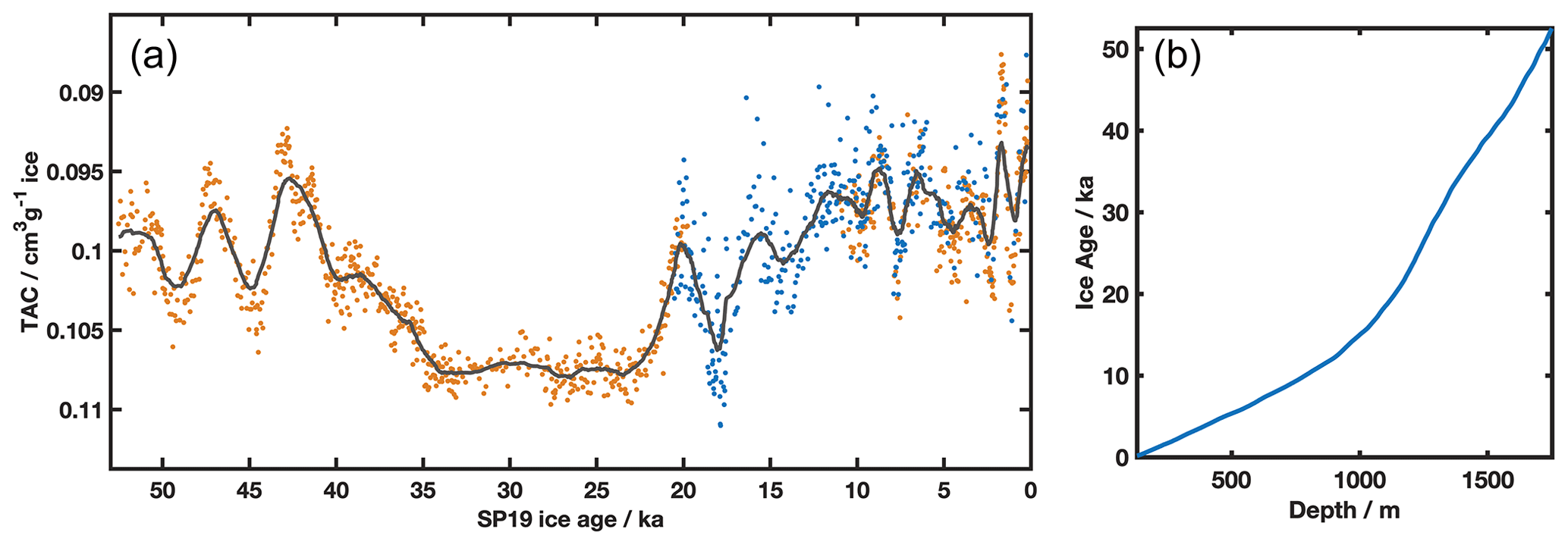
Figure 1 Total air content of the SPC14 ice core. (a) Measurements are individually shown, plotted on the SP19 ice age scale (Winski et al., 2019). Black line is the smoothed record using a running 10-point average. TAC is expressed in units of cubic centimeter (cm³) of air at standard temperature and pressure per gram of ice. Orange markers are TAC measurements collected at OSU (depths 130–841 and 1150–1751 m, pooled standard deviation = 0.0006 cm³ g⁻¹). Blue markers are TAC measurements collected at PSU (depths 130–1150 m, pooled standard deviation = 0.002 cm³ g⁻¹). (b) Ice age as a function of depth. Data are from Winski et al. (2019).

2 Materials and methods

2.1 Total air content measurements

The total air content (TAC) record from the SPC14 ice core was measured jointly in the Oregon State University (OSU) and Pennsylvania State University (PSU) ice core labs concurrently with measurements of CH₄. The core was discretely sampled at approximately 1 to 2 m resolution. Methods followed previous work (Epifanio et al., 2020; Mitchell et al., 2011; Lee et al., 2020; Buizert et al., 2021) with some calibration updates described below. At OSU, the samples were measured in accordance with previously published methods (Mitchell et al., 2015; Buizert et al., 2021). The PSU samples were also measured concurrently with CH₄, using a wet-extraction system. The differences in methods between OSU and PSU wet-extraction systems are described in Mischler et al. (2009), Fegyveresi (2015), Epifanio et al. (2020), and WAIS Divide Project Members (2013). Updates to the methods at OSU allow for a simple correction to the TAC measurements for variations in flask and array temperatures and volumes. The methods allowing this are described in detail below.

The OSU vacuum line is set up as portrayed in Fig. 2. Samples are melted under vacuum in a two-sided array of 12 glass vacuum flasks. The air released during the melt step is trapped in the headspace of the flasks. The melted samples are then refrozen in a −70 ^∘C ethanol bath. Once samples are refrozen, the air trapped in the flask headspace is expanded through the array volume, isolation volume, and the gas chromatograph (GC) sample loop. In the equations below, the quantity of air in the entire vacuum line (in moles) at this point is designated n₁. The relevant array valve is then closed, trapping air upstream of the isolation and GC volumes (Fig. 2). This quantity of air is designated n₂. The pressure in the GC volume is recorded by a capacitance manometer (rated at 0–100 torr, 1.5 % accuracy, P₁) The air in the GC sample loop is then injected into the GC column and measured for CH₄ concentration using a 6890N Agilent gas chromatograph with flame ionization detector. Once the analysis is complete, the gas remaining in the GC and isolation volumes (Fig. 2) is evacuated. The remaining air from the relevant array is then expanded into the GC section, and the relevant array valve is then again closed, trapping air upstream of the isolation and GC volumes (Fig. 2). In total, we make four expansions and four measurements of CH₄ concentration, and we made four measurements of GC pressure per sample. We assume that the temperatures of the vacuum line and GC do not change during the repeated expansions. TAC is derived from the sample mass and pressure measurements during the analysis, following the ideal gas law:

$$\begin{array}{}\text{(1)}& n={\displaystyle \frac{PV}{R{T}_{\mathrm{eff}}}},\end{array}$$

where P is pressure, V is volume, n is moles of air, T_eff is effective temperature (K) or weighted mean temperature of the various sections of the vacuum line, and R is the universal gas constant, 8.314 J mol⁻¹ K⁻¹.

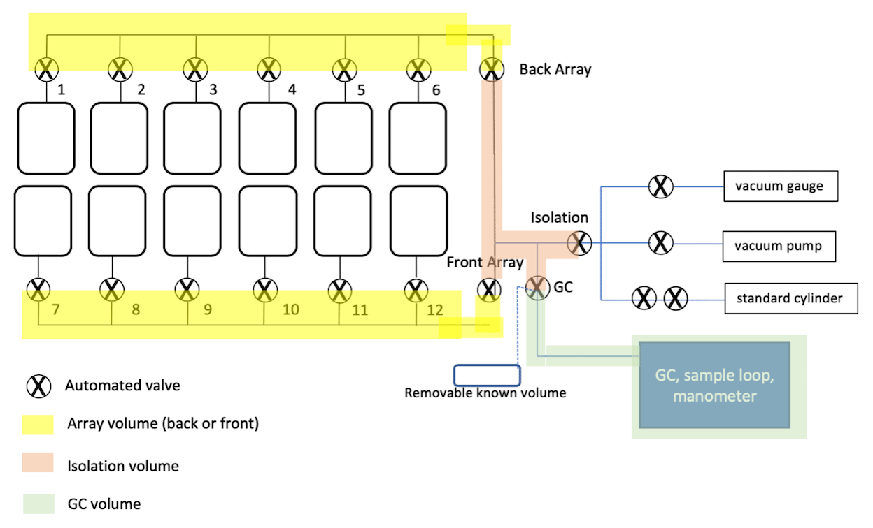
Figure 2 Schematic of extraction line and GC for TAC and CH₄ measurements. Diagram includes a removable known volume, which was used in the T_eff calibration (see the main text). Numbered valves are individual flask valves. Air released during the melt phase is trapped between the flask and the numbered automated valve. Yellow: back and front array volumes. Light orange: isolation volume, which includes the vacuum line between the array valves, the isolation valve, and the GC valve. Green: GC volume, which includes the vacuum line between the GC valve and the GC sample loop. All volumes are listed in Table 1.

The effective temperature of the line can change from day to day due to differences in air temperature, ethanol bath temperature, chiller efficiency, and flask headspace variation due to sample size. Because of the daily variation, it is problematic to use a weighted average calculation of T_eff in our calculation of TAC, as this would require a daily estimate of T_eff or an assumption that it is constant. To avoid this issue, we take advantage of the methods for CH₄ measurement. During the CH₄ measurement, we expand the air released from the melted ice in four expansions, with each subsequent expansion releasing lower pressures from the flask headspace. The ratio between the subsequent expansion pressures allows us to calibrate the TAC measurement, as follows.

Because the amount of air in the first expansion is equal to the amount in the second expansion plus what was removed by evacuation:

$$\begin{array}{}\text{(2)}& n_{\mathrm{1}}=n_{\mathrm{2}}+n_{\mathrm{rem}},\end{array}$$

where n₁ is the amount of air in the line during the first expansion, n₂ is the amount of air in the line during the second expansion, and n_rem is the amount of air removed in the first expansion. And

$$\begin{array}{}\text{(3)}& n_{\mathrm{1}}={\displaystyle \frac{P_{\mathrm{1}}{V}_{\mathrm{T}}}{R{T}_{\mathrm{eff}}}},n_{\mathrm{2}}={\displaystyle \frac{P_{\mathrm{2}}{V}_{\mathrm{T}}}{R{T}_{\mathrm{eff}}}},n_{\mathrm{rem}}={\displaystyle \frac{P_{\mathrm{1}}{V}_{\mathrm{gc}}}{R{T}_{\mathrm{gc}}}},\end{array}$$

where P₁ is the pressure of the first expansion, V_T is the total volume of the vacuum line and GC, and V_gc and T_gc are the volume and temperature of the vacuum line past the GC valve. Following from Eq. (2),

$$\begin{array}{}\text{(4)}& {\displaystyle \frac{P_{\mathrm{1}}{V}_{\mathrm{T}}}{R{T}_{\mathrm{eff}}}}-{\displaystyle \frac{P_{\mathrm{2}}{V}_{\mathrm{T}}}{R{T}_{\mathrm{eff}}}}={\displaystyle \frac{P_{\mathrm{1}}{V}_{\mathrm{gc}}}{R{T}_{\mathrm{gc}}}}.\end{array}$$

By rearranging to solve for $\frac{T_{\mathrm{gc}}}{V_{\mathrm{gc}}}$,

$$\begin{array}{}\text{(5)}& {\displaystyle \frac{T_{\mathrm{gc}}}{V_{\mathrm{gc}}}}={\displaystyle \frac{T_{\mathrm{eff}}{P}_{\mathrm{1}}}{V_{\mathrm{T}}(P_{\mathrm{1}}-P_{\mathrm{2}})}},\end{array}$$

and then by rearranging to solve for T_eff,

$$\begin{array}{}\text{(6)}& T_{\mathrm{eff}}=V_{\mathrm{T}}{\displaystyle \frac{P_{\mathrm{1}}-P_{\mathrm{2}}}{P_{\mathrm{1}}}}{\displaystyle \frac{T_{\mathrm{gc}}}{V_{\mathrm{gc}}}}.\end{array}$$

TAC is calculated by dividing n₁ by sample mass. To eliminate the need to measure T_eff every time TAC is calculated, we use Teff from Eq. (6) in the calculation of TAC:

$$\begin{array}{}\text{(7)}& {\displaystyle \frac{n_{\mathrm{1}}}{m}}={\displaystyle \frac{P_{\mathrm{1}}^{\mathrm{2}}}{R(P_{\mathrm{1}}-P_{\mathrm{2}})}}{\displaystyle \frac{T_{\mathrm{gc}}}{m{V}_{\mathrm{gc}}}}.\end{array}$$

We then substitute R in Eq. (7) for the ideal gas law, with a final calculation for TAC:

$$\begin{array}{}\text{(8)}& \mathrm{TAC}={\displaystyle \frac{P_{\mathrm{1}}^{\mathrm{2}}}{R(P_{\mathrm{1}}-P_{\mathrm{2}})}}{\displaystyle \frac{T_{\mathrm{gc}}{T}_{\mathrm{STP}}}{m{V}_{\mathrm{gc}}{P}_{\mathrm{STP}}}}.\end{array}$$

For comparison to previous work, we convert to units of cm³ g⁻¹ at standard temperature and pressure (STP) conditions. Equation (8) requires that we have an accurate measure of $\frac{T_{\mathrm{gc}}}{V_{\mathrm{gc}}}$. Two separate methods were used to achieve this. The first method involved estimating T_eff by taking a weighted average of the system temperature with the GC oven at 50 ^∘C and the flasks submerged in a −70 ^∘C ethanol bath. Once a known amount of air was expanded into the GC, $\frac{T_{\mathrm{gc}}}{V_{\mathrm{gc}}}$ was calculated. The line temperature for the portion outside the GC oven was estimated by averaging the measured temperature at multiple points adjacent to the line. The variation in temperature of the line was less than 0.1 ^∘C. The final value of $\frac{T_{\mathrm{gc}}}{V_{\mathrm{gc}}}$ determined using this method was 12.37 K cm⁻³.

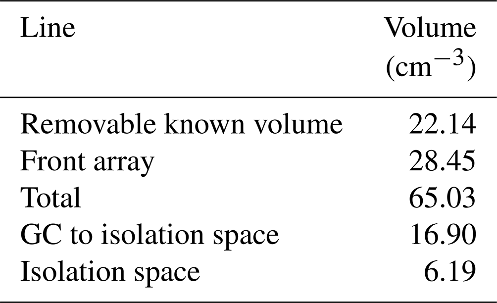
The second calibration did not use the chilled flasks and instead utilized a removable known volume of air that was externally attached to the vacuum line. From expansions of air to other parts of the array and GC, we were able to calculate the volume of the entire system, individual components, and the GC. All volumes are listed in Table 1. Air was expanded into the entire system at a known pressure, with the GC at room temperature (21.5 ^∘C). The front array valve was closed, isolating the pressure in the front array, while the rest of the line was pumped to vacuum. After the pressure stabilized, the air in the front array was expanded to the entire line, and the pressure was recorded. Finally, the GC oven was switched on and raised to the normal operating temperature (50 ^∘C). The pressure in the total line after heating was recorded as P_eff. To solve for T_eff, we use the combined gas law:

$$\begin{array}{}\text{(9)}& {\displaystyle \frac{P_{\mathrm{1}}{V}_{\mathrm{1}}}{T_{\mathrm{1}}}}={\displaystyle \frac{P_{\mathrm{2}}{V}_{\mathrm{2}}}{T_{\mathrm{2}}}}\end{array}$$

where P₁=P_array is the pressure of the air in the front array with the line at room temperature; V₁=V_array is the volume of the front array; T₁ is the measured lab temperature; P₂=P_eff or the pressure of the air in the entire system, including both array volumes, isolation volume, and the GC volume; and T₂=T_eff or the effective temperature of the entire system with the GC at 50 ^∘C. Rearranging Eq. (9) to solve for T₂ (or T_eff), we get

$$\begin{array}{}\text{(10)}& T_{\mathrm{eff}}={\displaystyle \frac{P_{\mathrm{eff}}{V}_{\mathrm{T}}{T}_{\mathrm{array}}}{P_{\mathrm{array}}{V}_{\mathrm{array}}}}\end{array}$$

Finally, multiple expansions of air from the front array to the GC volume consistently give a ratio of pressures (between the four subsequent expansions for one measurement) of 0.56. Combined with Eq. (5); this ratio yields a final $\frac{T_{\mathrm{gc}}}{V_{\mathrm{gc}}}$ of 12.79 K cm⁻³. This value is different from the original value of 12.37 K cm⁻³, but we believe it is more accurate due to the difficulty of estimating T_eff during the first calibration. The second method also removes the variability of flask size and accounts for small changes made in the vacuum line over time. All measurements of TAC on the SPC14 ice core were calibrated using the $\frac{T_{\mathrm{gc}}}{V_{\mathrm{gc}}}$ value of 12.79 K cm⁻³.

Table 1 Volumes of CH₄ extraction line. Volumes listed correspond to highlighted areas in Fig. 2.

2.2 Solubility and cut-bubble corrections

Two small corrections were made to the TAC measurements to account for effects on TAC introduced during sample preparation and measurement. Because the air trapped in the headspace of the flask is not allowed sufficient time to reach solubility equilibrium during the melt–refreeze process, a correction was made to account for the residual gas trapped in the refrozen ice. Following Mitchell et al. (2015), we determined an empirical TAC solubility correction of +1.3 %, which we added to all sample measurements. This empirical correction was derived during wet extraction by measuring the TAC remaining within the flask headspace after a second melt–refreeze cycle.

The second correction accounts for the air lost during cutting and trimming of the ice samples. Preparing ice core samples for measurement unavoidably cuts through some bubbles, releasing a fraction of the air content from the entire ice sample. As a result, measurements made of the total air are slightly lower than true values.

This cut-bubble correction is based on a statistical relationship between the total number and average size of bubbles in a given sample, as well as the amount of exposed surface area that is cut during sample preparation (Saltykov, 1976). Bubble numbers and average sizes were determined during number-density, physical property, and micro-CT measurements as described in Fegyveresi et al. (2011), Fitzpatrick et al. (2014), and Fegyveresi et al. (2018). Following the methods in Martinerie et al. (1990) and Fegyveresi (2015), we interpolated the bubble size and density to each TAC sample, and we applied the correction based on the bubble size distribution for each sample across the dataset. To estimate the exposed surface area of each sample, we used the standard rectangular dimension (2.5 cm × 2.5 cm × 9 cm) and a mass of 51.2 g across all samples. There is likely some missed variation due to trimming on the edge of samples, but the variation is small. The cut-bubble correction indicates a maximum of 8 % loss in the first 200 m of ice, decreasing to 1.9 % TAC loss at the base of the bubbly ice at ∼1200 m, at the onset of the clathrate-ice transition. The correction is shown in Fig. 3. While clathrate ice will still have a gas-loss correction, it is likely constant and no more than 1.9 %. We applied no correction below the base of the bubbly ice.

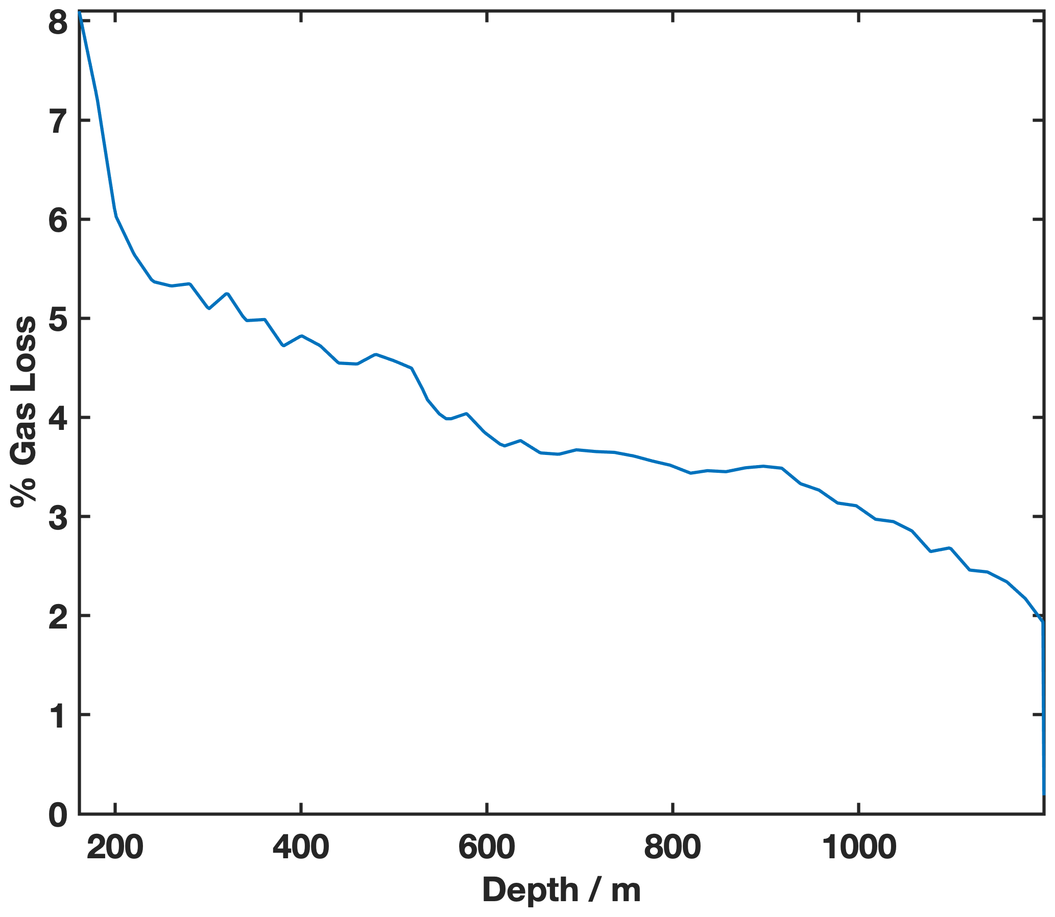
Figure 3 Cut-bubble correction for SPC14 ice core. Gas loss plotted with depth on the SPC14 ice core. Cut-bubble corrections range from 8 % decreasing to 1.9 % gas loss at the base of the bubbly ice.

3 Results and discussion

3.1 South Pole total air content record

The SPC14 ice core TAC record is shown in Fig. 1, plotted on the SPC19 ice age scale (Winski et al., 2019). We plot our data on the ice age scale rather than the gas age scale, given evidence that ice sheet surface conditions have a major impact on the pore volume at bubble close-off (further discussed below). This convention is consistent with previous research (Eicher et al., 2016; Raynaud et al., 2007). Using the method described above, we measured TAC concurrently with the SPC14 CH₄ (Epifanio et al., 2020), resulting in a total of 2318 measurements made on samples at 1067 individual depths. Samples were taken at approximately every meter along the depth range from 131 to 1751 m, which spans the period of 130 to 54 302 years BP. The age resolution of these samples is the same as reported for CH₄ in the SPC14 ice core, averaging 42 years, but increasing from 20 years in the Holocene to 190 years at the bottom of the ice core record (Epifanio et al., 2020).

The OSU dataset has a pooled standard deviation of 0.0006 cm⁻³ g⁻¹, and the PSU dataset (130–1150 m) has a pooled standard deviation of 0.002 cm⁻³ g⁻¹. Differences in methods between the OSU and PSU labs created a mean offset of 0.0072 cm³ g⁻¹. To correct for this offset, PSU values were increased to be comparable to OSU values. The pooled standard deviation of measurements for the combined dataset (130–1150 m) is 0.002 cm⁻³ g⁻¹, and data from 1151–1751 m have a pooled standard deviation of 0.001 cm⁻³ g⁻¹. Data are available at the U.S. Antarctic Program (USAP) data repository (https://doi.org/10.15784/601546), including the details of uncertainties and sample resolution of datasets (Epifanio et al., 2022). To our knowledge, this is the first ice core TAC record with this resolution and length, allowing in-depth comparison with other climate proxies at a site that is not likely to have experienced significant elevation change over the last 54 kyr (Fudge et al., 2020; Lilien et al., 2018).

The SPC14 TAC record has several notable characteristics (Fig. 1). Long-term trends include an increase in TAC from 53 to 36 ka, followed by an approximately 10 kyr period of low variability, then decreasing TAC from about 20 ka to the present. Millennial-scale variations, both in the Holocene and glacial period, consist of large-magnitude abrupt changes. These variations are as large as 0.007 cm⁻³ g⁻¹ in 2600 years, which is 47 % of the total amplitude in the record. Higher frequency variations exist on centennial or shorter timescales that may represent firn processes such as layering, but our sampling resolution is not adequate to fully evaluate this possibility.

3.2 Impacts of temperature on TAC

Prior work suggests that temperature impacts TAC in two ways: the first through the ideal gas law and the second through an empirically established relationship between the pore volume at bubble close-off and temperature (Martinerie et al., 1992). Given a fixed pore volume at close-off, TAC is given by the ideal gas law:

$$\begin{array}{}\text{(11)}& \mathrm{TAC}=V_{\mathrm{c}}\cdot {\displaystyle \frac{P_{\mathrm{c}}}{T_{\mathrm{c}}}}\cdot {\displaystyle \frac{T_{\mathrm{0}}}{P_{\mathrm{0}}}},\end{array}$$

where TAC is the total air content (cm⁻³ g⁻¹), V_c is the pore volume at close-off (cm³g⁻¹), P_c and T_c are pressure and temperature of the air contained in V_c at close-off (mbar and K), and P₀ and T₀ are standard pressure and temperature (1013 mbar and 273 K, respectively).

The empirical relationship between pore volume and temperature, as found by Martinerie et al. (1992), is given by

$$\begin{array}{}\text{(12)}& V_{\mathrm{c}}=\mathrm{7.6}\times {\mathrm{10}}^{-\mathrm{4}}\cdot T_{\mathrm{s}}-\mathrm{0.057},\end{array}$$

where T_s is the surface temperature (K).

To examine direct thermal effects, we follow Raynaud et al. (2007) and Eicher et al. (2016) to define a non-thermal residual term V_cr:

$$\begin{array}{}\text{(13)}& V_{\mathrm{cr}}=\mathrm{TAC}\cdot {\displaystyle \frac{T_{\mathrm{c}}}{P_{\mathrm{c}}}}\cdot {\displaystyle \frac{P_{\mathrm{0}}}{T_{\mathrm{0}}}}-V_{\mathrm{c}}.\end{array}$$

We use the same temperature for the surface (T_s) and the close-off depth (T_c). While the temperature at pore close-off (T_c) is a bit warmer than T_s due to geothermal heating, the difference is small when the firn column is in equilibrium. For the temperature at bubble close-off (T_c), we used a temperature reconstruction from Kahle et al. (2021). To approximate P_c, we use a value of 680 mbar at the surface of the ice core, linearly decreasing with depth to account for 180 m of elevation increase upstream of the drill site (NOAA, US Department of Commerce, Global Monitoring Laboratory, 2021; Fudge et al., 2020).

Following Raynaud et al. (2007) and Lipenkov et al. (2011), we then create standardized versions of TAC and V_cr, called TAC^* and $V_{\mathrm{cr}}^{*}$, in order to compare TAC and the non-thermal residual. The standardized datasets were created by subtracting the mean value (of TAC or V_cr, respectively) and then dividing by the respective standard deviation. These data are plotted together in Fig. 4. The correlation between TAC^* and $V_{\mathrm{cr}}^{*}$ is very high (r²=0.96). This is because $V_{\mathrm{cr}}^{*}$ is a quantity that describes TAC if temperature did not affect pore volume at close-off, and it is useful for understanding the magnitude of the direct effects of temperature. The very high correlation between TAC^* and $V_{\mathrm{cr}}^{*}$ agrees with previous work on both European Project for Ice Coring in Antarctica Dome C (EDC) and North Greenland Ice Drilling Project (NGRIP) ice cores that show the direct temperature effect on TAC is responsible for a very small amount of TAC variability. As a result, we targeted our analysis using measured TAC instead of the non-thermal residual.

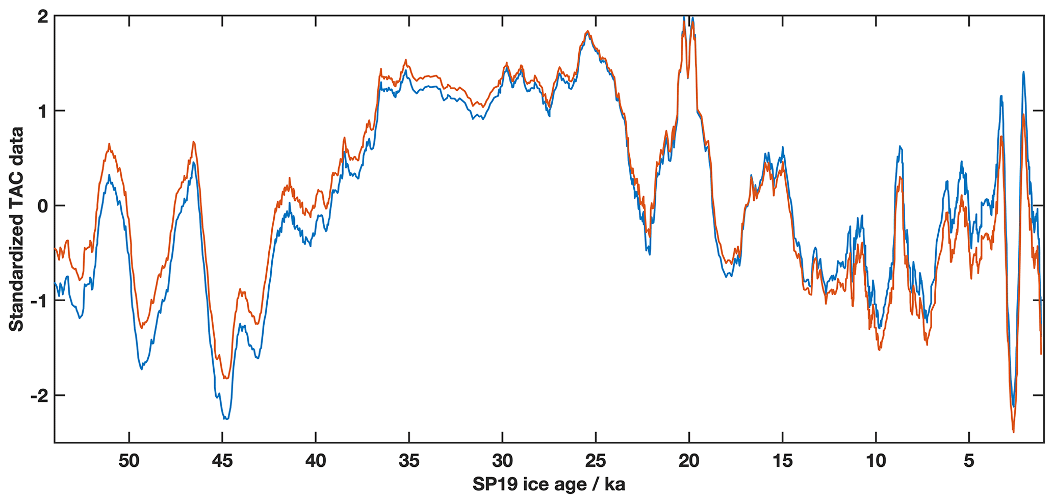
Figure 4 Comparison of TAC and the non-thermal residual. The non-thermal residual quantity, explained in Sect. 3.2, explains how much temperature affects TAC. The TAC and non-thermal residual are nearly identical, indicating a very small direct effect of temperature on TAC. Blue: a standardized version of the SPC14 TAC record. Orange: following Raynaud et al. (2007), the standardized TAC data after correcting for the direct effects of temperature (V_cr) (Martinerie et al., 1992). Both records were smoothed using a 10-point moving average to better highlight the difference.

3.3 Orbital-scale variations in TAC

Local integrated summer insolation (ISI) has shown an anti-correlation with TAC in various Antarctic and Greenland ice cores (Raynaud et al., 2007; Lipenkov et al., 2011; Eicher et al., 2016). The South Pole is an interesting site to study in this regard, as it is the only place in Antarctica without a diurnal cycle in solar insolation. Following Huybers et al. (2006) and Raynaud et al. (2007), we find ISI by

$$\begin{array}{}\text{(14)}& \mathrm{ISI}=\sum {\mathit{\beta }}_{\mathrm{i}}({\mathit{\omega }}_{\mathrm{i}}\cdot \mathrm{86}\mathrm{400}),\end{array}$$

where ISI is in joules, ω_i is the daily insolation in W m⁻², and β_i is a Heaviside step function where β_i= 1 when ω_i is > ω_threshold; otherwise, β_i=0. ISI is impacted by a mix of precession and obliquity, and the curves are unique for latitude and the chosen ω_threshold

Earlier research emphasized the anti-correlation between ISI and TAC and uses the relationship to orbitally tune the ages of Antarctic ice core records (Lipenkov et al., 2011; Raynaud et al., 2007; Parrenin et al., 2007). Conclusions of a previous study suggest that the insolation effect is much larger than the direct effects of temperature discussed above and is found in both Northern Hemisphere and Southern Hemisphere records (Eicher et al., 2016).

We find a maximum anti-correlation of ISI with TAC at a cutoff threshold of 225 W m⁻² (r²= 0.46, p < 0.0001). Studies of the same relationship in the EDC and NGRIP ice cores found maximum correlations at different cutoff values (390 W m⁻² for NGRIP with r²=0.3) (Eicher et al., 2016; Raynaud et al., 2007). However, the correlation difference between varying threshold values (0 to 500 W m⁻²) is small (r²= 0.42 to r²= 0.46). The linear regression of TAC as a function of ISI at a threshold cutoff of 225 W m⁻² is shown in Fig. 5. To make this calculation, we interpolated the ISI data to the ages assigned to TAC.

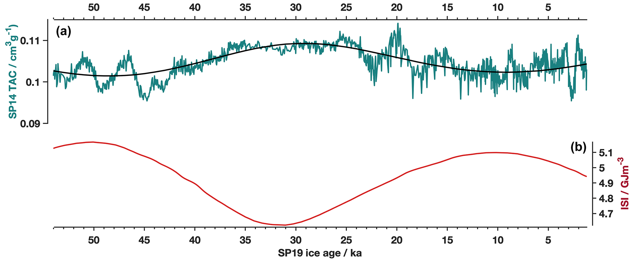
Figure 5 SPC14 TAC predicted from integrated solar insolation (ISI) (a) SPC14 TAC (green) and by linear regression of TAC with ISI using a cutoff threshold of 225 W m⁻². R²= 0.46, p < 0.0001, b= 0.194, $m=-\mathrm{0.0173}$. (b) ISI at 90^∘ S using a cutoff threshold of 225 W m⁻².

The ISI regression misfit values show an even distribution. The link between TAC and ISI supports the proposition that TAC can be used for absolute (orbitally tuned) dating of ice cores (Raynaud et al., 2007). It is worth noting, however, that the SPC14 TAC record only covers the last 54 000 years, which is only slightly longer than one obliquity cycle. This time period is shorter than the ice core records mentioned above, which may affect the differences in cutoff threshold that give maximum correlation between TAC and ISI.

3.4 Millennial-scale variations observed in TAC

While the ISI appears to be highly correlated with long-term variations in TAC, it fails to explain the observed millennial-scale changes. Abrupt, large-magnitude, millennial-scale variations in TAC exist through the Holocene and an early part of the glacial period. The approximate magnitude of the largest, abrupt, millennial-scale changes is 0.007 cm³ g⁻¹ in ∼3 kyr, which is similar to the abrupt millennial-scale variations observed in NGRIP, which were typically around 0.01 cm³ g⁻¹ in the same time frame (Eicher et al., 2016). Millennial-scale variations are absent from 40 to 22 ka in the SPC14 ice core, but high-frequency (centennial-scale and smaller) variations persist through the entire record. The existence of millennial-scale and higher frequency variations underscores the need for high-resolution data to discern the long-term patterns from other climatic effects on TAC. We isolate the millennial-scale TAC variations by subtracting the orbital-scale trends that we find via regression of TAC onto ISI (Fig. 5). The largest millennial-scale features occur at 52, 46, and 44 ka. Similar large features are not found between 43 and 25 ka, where the TAC reaches a maximum steady value of about 0.11 cm³ g⁻¹. Large variations resume at 22 ka and occur through the Holocene time period, mostly between 9 and 2 ka.

We first investigate the possibility of surface pressure changes driving the millennial-scale variability. Using the relationship of air pressure with TAC (Eq. 11), as proposed by Martinerie et al. (1992), we calculated the pressure change required for a representative high-frequency TAC change. For example, the abrupt increase in TAC of 0.01 cm³ g⁻¹ in 2.7 kyr starting at 49.2 ka (Fig. 1) would require a mean pressure change of 104 hPa over that time interval. In the absence of elevation change, central Eastern Antarctica could not likely sustain large atmospheric pressure changes for that length of time. Hourly atmospheric pressure measurements at the South Pole are between 710 and 650 hPa, varying on seasonal timescales (NOAA, US Department of Commerce, Global Monitoring Laboratory, 2021). However, daily, or even seasonal, variations in pressure are not likely to be recorded in our TAC record due to the gradual bubble trapping process that takes decades to complete. Current spatial gradients of sea level pressure, including variations associated with the Amundsen Sea Low (ASL), show a maximum range of about 50 mbar from maximum low to high pressure over Antarctica (Schneider et al., 2012; Raphael et al., 2016). A change in atmospheric pressure large enough to explain these TAC variations would require a dramatic reorganization of the westerly winds, which is highly unlikely during the last glacial period. Some modeling studies have examined wind changes around Antarctica, using 10 000-year model runs, and found moderate changes in sea level pressure, no greater than 15 hPa (Goodwin et al., 2014). The wind effect, as described in Martinerie et al. (1994), would require large sustained wind changes over millennia that are not supported by modeling reconstructions (Goodwin et al., 2014).

If the TAC changes were entirely explained by a surface pressure change induced from ice sheet elevation changes, an elevation change of about 1200 m would be needed. Such a large and abrupt change is unlikely to have been driven by accumulation change alone and is otherwise not likely due to the geographical context of the South Pole. Accumulation rates during the glacial period were just 3 cm yr⁻¹ (water equivalent), which would mean the maximum amount of elevation gain due to accumulation alone would be only about 80 m, without considering the effects of ice layer thinning.

The location of SPC14 in the interior of Eastern Antarctica means that it would not have been subject to large elevation changes associated with major climate transitions, especially during the beginning of the last glacial period (Golledge et al., 2013; Fudge et al., 2020). The SPC14 ice core was not drilled at an ice divide, which means the ice collected at the South Pole flowed over topography before it arrived at the sampling location. This flow changed the local elevation at which the snow fell in the past. The history of ice flow of the SPC14 ice core, however, is not constrained beyond 100 km from the core site and is best constrained in the closest 65 km, representing the last 10 kyr, or about 725 m ice core depth (Lilien et al., 2018; Fudge et al., 2020). Following the ice flow line upstream from the modern ice core site shows the bedrock elevation only varying by about 500 m, which corresponds to an ice surface elevation variation of about 300 m during that time (Lilien et al., 2018; Fudge et al., 2020; Kahle et al., 2021; Morgan et al., 2022). This 300 m change is much less than the 1200 m change required by our millennial-scale TAC observations. Large transient features in surface ice sheet elevation do not exist, eliminating ice flow as a source of abrupt elevation change influencing TAC.

Other hypotheses for changing TAC include layering due to melt and dust affecting grain metamorphism. Layering due to melt (or other effects) influences the trapping of air in ice, shaping TAC, but it is not relevant here due to the lack of melt layers. Dust has also been documented to influence grain metamorphism in the firn. Due to its interior location, the ice at the South Pole experiences very small changes in dust flux. We observe no correlation between dust deposition and TAC.

3.4.1 Accumulation

Since we can reasonably show that large millennial-scale changes in TAC are not due to direct effects of temperature, variations in air pressure, or ice dynamics, pore volume at bubble close-off must account for most of the TAC variations. Two observations are important to help explain these changes as a function of pore volume at close-off: (1) a positive correlation between TAC and accumulation rate and (2) a high positive correlation between TAC and δ¹⁵N-N₂ in trapped air in the core.

First, the millennial-scale changes in TAC are highly correlated with the accumulation rate reconstruction from Kahle et al. (2021), also plotted on the SP19 ice age (r²= 0.59, p < 0.001, Fig. 6 and Table 2). Kahle et al. (2021) calculated the accumulation rate by using an inverse method which used models of firn densification, water isotope diffusion, and layer thinning to predict an accumulation rate history based on constraints provided by measured Δage, diffusion length, and annual layer thicknesses. The first 11.3 kyr of the Kahle et al. (2021) reconstruction incorporates measured annual layer thicknesses from the layer-counted timescale from Winski et al. (2019). This results in an accumulation record that closely resembles the previous accumulation rate history from Winski et al. (2019) for this section of the core.

Table 2 Pearson correlation coefficients of single regressions. High-pass filtered records were filtered using a bandpass filter that eliminated frequencies greater than 10 000 years.

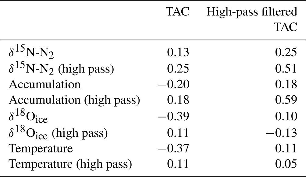
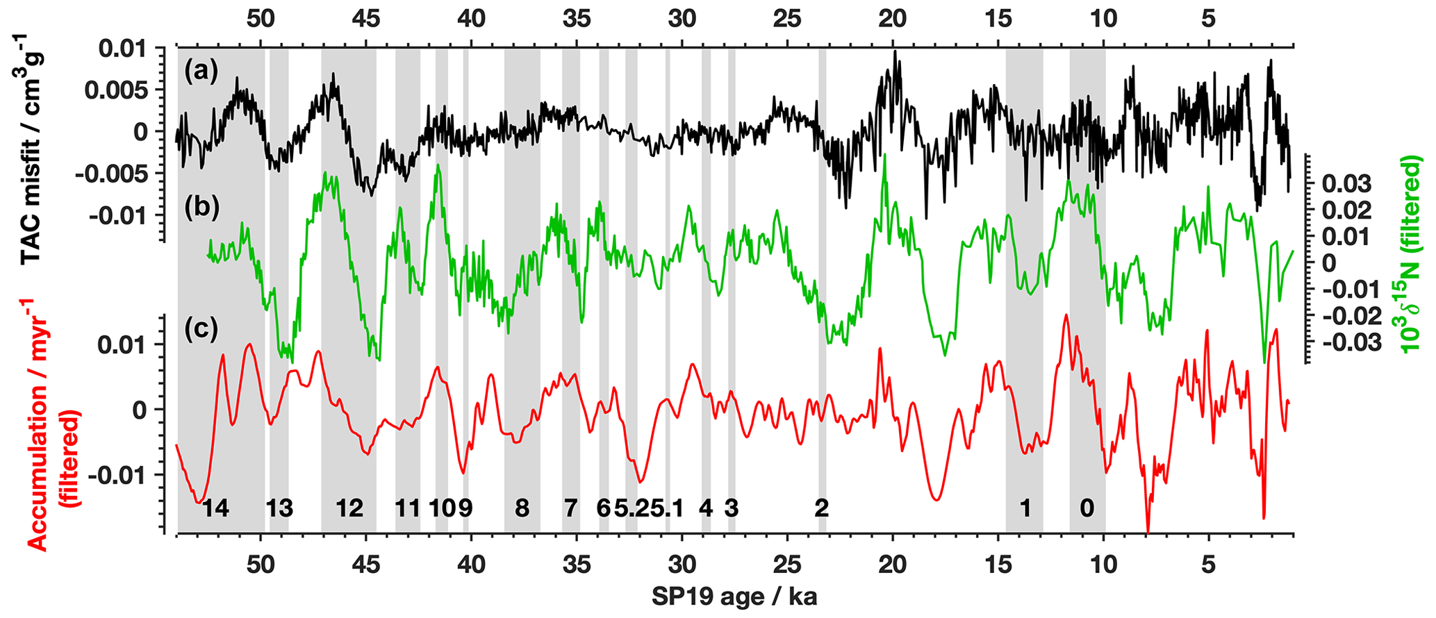
Figure 6 TAC, accumulation rate, and δ¹⁵N-N₂. TAC misfit (black, a) compared with δ¹⁵N-N₂ (green, b; Winski et al. (2019)) accumulation rate (red, bottom; Kahle et al., 2021). Both δ¹⁵N-N₂ data and accumulation rate were filtered using a high-pass filter, removing variability with a period greater than 10 000 years prior to comparison. TAC misfit was plotted on the SP19 ice age scale. The high-pass filtered δ¹⁵N-N₂ data are plotted on the SP19 gas age scale (middle; Epifanio, 2022). The high-pass filtered accumulation rate on the SP19 ice age scale (c; Winski et al., 2019). Grey shaded areas are Dansgaard–Oeschger (D–O) events, numbered on the bottom for reference. Correlation coefficients are presented in Table 2.

Second, the millennial-scale changes in TAC are also highly correlated with δ¹⁵N-N₂ when plotted on the SP19 gas age scale (r²= 0.51, p < 0.001, Fig. 6 and Table 2). This observation is consistent with the idea that millennial-scale fluctuations in accumulation drive similar-scale changes in firn thickness, which affects δ¹⁵N-N₂ due to gravitational fractionation (Severinghaus et al., 1998; Sowers et al., 1992; Morgan et al., 2022). As temperature variations are relatively minor at the South Pole, it is accumulation variation that drives the observed changes in SPC14 δ¹⁵N-N₂. At this site, greater accumulation rates cause a thicker firn column and a subsequently higher δ¹⁵N-N₂. Because δ¹⁵N-N₂ is not set until pore close-off, toward the base of the firn, comparison of the effect on δ¹⁵N-N₂ with accumulation rate is done using the gas age scale for δ¹⁵N-N₂ and the ice age scale for TAC. Winski et al. (2019) also notes the close resemblance of δ¹⁵N-N₂ and the Holocene accumulation rate reconstruction, which is further evidence to support the use of δ¹⁵N-N₂ as an indicator of accumulation rate changes in SPC14. TAC was compared with temperature reconstructions as well as δ¹⁸O_ice. Low r values were recorded, and the results are listed in Table 2. Note that Kahle et al. (2021) do not use δ¹⁵N-N₂ in their inversion method.

Metamorphism of the ice in the first few meters of the firn may explain the link between accumulation rate and TAC. Lower accumulation rates allow grains to remain at or near the surface for a longer time, giving grains in the firn more time to grow while they remain at the surface (Courville et al., 2007). The size of the firn grains at the surface seems to predict at which density bubble close-off occurs, with larger-grained firn closing off at a higher density (Arnaud, 1997; Gregory et al., 2014). Because ice density is, by definition, inversely proportional to porosity, higher-density bubble close-off (associated here with longer time near the surface of the ice sheet, larger grain sizes, and lower accumulation) leads to bubbles with less pore volume than firn with smaller grain sizes. Lower accumulation rates may additionally allow more time for grains to become spherically shaped, before close-off, where higher accumulation rates tend to close off bubbles earlier in the densification process. Because grains tend to move toward a spherical shape with enough time, due to vapor diffusion (Eicher et al., 2016), low accumulation rates create more homogeneous, spherically shaped grains. These spherically shaped grains could force more air to escape the ice core, leading to lower TAC. Gregory et al. (2014) noted higher gas diffusivity at lower accumulation sites, implying that at low accumulation sites, the pores are closing off later, allowing time for more spherically shaped grains. We propose that a mechanism of grain size and shape affecting pore volume leads to a positive correlation between accumulation and TAC, which we observe in the SPC14 ice core; however, the microstructure and physics behind the mechanism should be explored in future work.

In a sense, this proposed grain size mechanism is similar to the proposed mechanism for how ISI impacts TAC on an orbital timescale (Raynaud et al., 2007; Eicher et al., 2016). ISI is hypothesized to act on TAC by changing the grain size of the firn at the surface by influencing temperature gradients in the first few meters of firn. On orbital timescales, higher ISI increases the near-surface firn metamorphism and grain size and decreases pore volume at close-off, resulting in the inverse relationship between TAC and ISI recorded in both hemispheres (Raynaud et al., 1997; Eicher et al., 2016). In our proposed mechanism for millennial-scale variations in TAC, lower accumulation increases near-surface firn metamorphism and grain size and decreases pore volume at close-off. In both scenarios (orbital- and millennial-scale changes), grain size is set in the first few meters of the firn, though by different mechanisms, and the impact is advected to the close-off depth. We propose that the relationship between grain size and accumulation rate is responsible for the large, millennial-scale changes in TAC found in the SPC14 ice core. This mechanism is complementary to the orbital changes in TAC imposed by ISI and creates millennial-scale changes imposed on top of orbital-scale changes.

Studies of TAC in Greenland suggest a different mechanism for similar-magnitude changes in TAC. Eicher et al. (2016) observed a complex, asynchronous relationship between rapid climate changes (D–O events) and millennial-scale TAC changes in the NGRIP ice core. Figure 7 shows the Greenland (North GRIP) TAC record compared with accumulation at the same site. Eicher et al. (2016) suggest the relationship is due to step changes in accumulation rate and temperature during D–O events in Greenland, causing the firn to densify rapidly due to increased load changes. This hypothesis is not consistent with our results in the SPC14 ice core, perhaps because the load changes in Antarctica are not nearly as large or abrupt as observed in Greenland. Accumulation rate changes at the South Pole during the glacial period are much smaller than in Greenland (1 cm yr⁻¹ or 25 % change over an Antarctic Isotope Maxima (AIM) event, compared with 10 cm yr⁻¹ or 100 % increase during a D–O event in Greenland), while the TAC changes at both locations are of a similar magnitude (0.007 cm³ g⁻¹ at SPC14, 0.005 cm³ g⁻¹ at NGRIP). This suggests that the accumulation effect on TAC scales differently at NGRIP when compared to SPC14, implying that the two locations respond differently to accumulation changes. Interpreting TAC at any ice core requires a universal explanation of how the firn densifies, and future work may elucidate a single mechanism that can explain the TAC–accumulation relationship at both polar regions. For example, we hypothesize that the grain size mechanism dominates at colder, dryer locations, and the mechanism requiring transient firn densification would prevail when warmer, wetter conditions exist. High-resolution TAC datasets across a suite of climate conditions are needed to test this hypothesis.

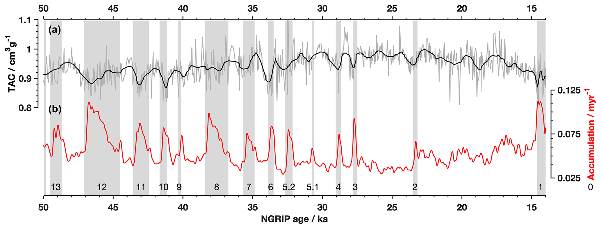
Figure 7 TAC and Greenland (NGRIP) TAC. TAC (grey, a; Eicher et al., 2016) compared with accumulation rate (red, b; Kindler et al., 2014). The Black line is smoothed TAC using a 10-point running average. Grey shaded areas are D–O events, numbered on the bottom for reference. Correlation coefficients are presented in Table 4.

3.5 Multiple regressions to further investigate controls on TAC

A multiple-regression analysis was performed to examine how climate-related variables correlate with TAC at SPC14. This analysis was performed to examine the possibility of removing non-elevation-dependent signals the record. Because we do not expect large elevation changes at the South Pole site, SPC14 is an excellent ice core to examine this possibility. If the TAC variability in the SP14 core can be explained using measured or modeled climate variables, it might be possible in future projects to extract the portion of the variability due to elevation change. Here we considered two separate multiple linear regression analyses. In the first multiple regression (referred to as the “modeled reconstruction” regression), we examined the relationship between TAC, ISI, and accumulation rate. In the second multiple regression (referred to as the “measured data” multiple regression), we examined the links between TAC, ISI, and δ¹⁵N-N₂. TAC data and variables considered are plotted in Fig. 8.

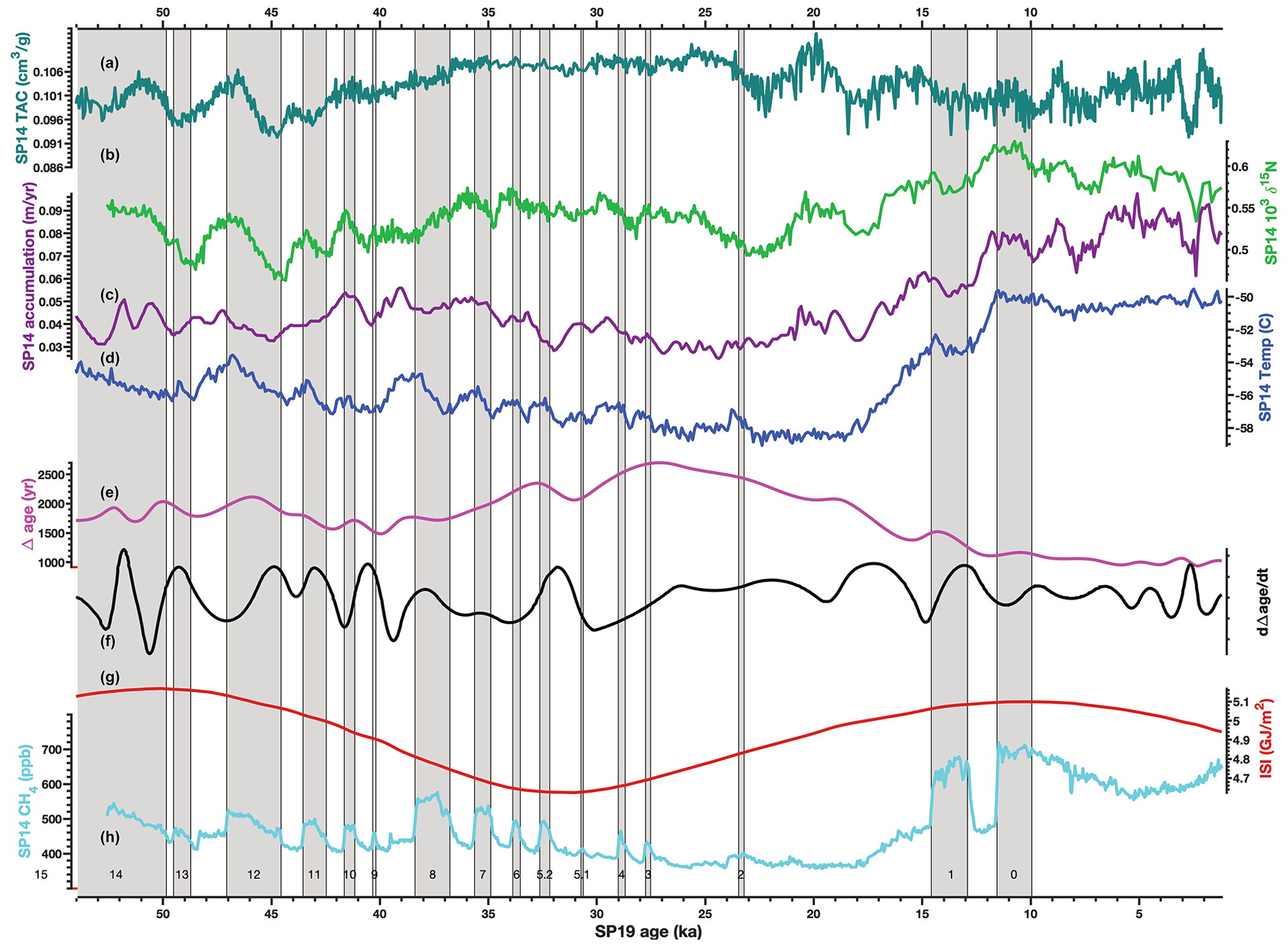
Figure 8 TAC record of SPC14 ice core and other climate proxies. (a) SPC14 TAC record. Mean value of duplicate measurements, plotted on the ice age scale. (b) δ¹⁵N-N₂, plotted on the gas age scale (Winski et al., 2019). (c) Accumulation rate plotted on the ice age scale. For the last 11.3 kyr, the accumulation rate was constrained by layer counting of seasonal variations of magnesium and calcium ions (Winski et al., 2019). For older time periods, accumulation was modeled using an inverse method (Winski et al., 2019; Kahle et al., 2021). (d) δ¹⁸O_ice a local temperature proxy (Kahle et al., 2021). (e) SPC14 Δage, empirically derived using independent gas and ice age markers (Epifanio et al., 2020) (f) Derivative of Δage. (g) Integrated summer insolation (ISI), at a cutoff threshold of 225 W m⁻², at 90^∘ S (Huybers et al., 2006). (h) SPC14 CH₄, plotted on the gas age scale, added for chronological orientation (Epifanio et al., 2020). Grey bars are numbered and represent D–O events for reference.

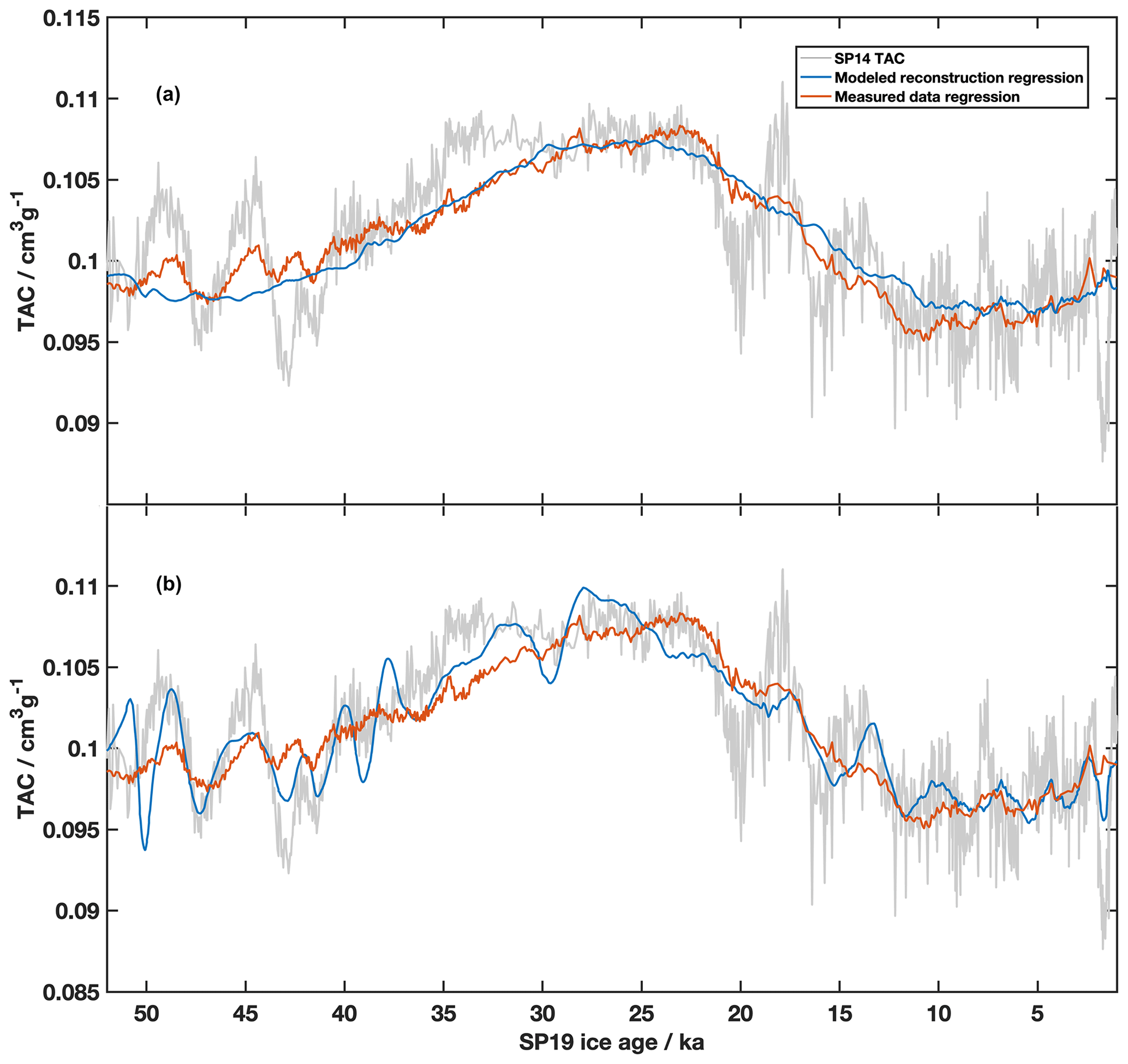
Figure 9 Multiple regressions of TAC compared to SPC14 TAC record. (a) SPC14 TAC data (grey); modeled reconstruction multiple regression, which used ISI and modeled reconstructions of accumulation rate (r²= 0.51, p < 0.001) (blue); measured data multiple regression, which includes δ¹⁵N-N₂ and ISI (r²= 0.62, p < 0.001) (orange). (b) Multiple-regression comparison including δΔage/δt. SPC14 TAC data (grey); multiple regression using modeled reconstructions of temperature and accumulation rate, including δΔage $/$ δt (r²= 0.76, p < 0.001) (blue); multiple regression using measured parameters, including δΔage $/$ δt (r²= 0.77, p < 0.001) (orange).

The modeled reconstruction regression included TAC, ISI, and the Kahle et al. (2021) reconstruction of accumulation rate. The modeled reconstruction multiple regression had a maximum adjusted r²= 0.51 (p < 0.0001); therefore, the combined relationship accounts for 51 % of the variation in the SPC14 TAC. The modeled reconstruction multiple-regression residuals show an even distribution. The parameters are listed in Table 3 in order of how much each parameter affected the adjusted correlation coefficient.

Table 3 Multiple regressions of TAC. The parameter listed is the term considered in the regression. Parameters are listed in the order of how much adjusted r² changes when the parameter is removed from the regression; (a) terms of multiple regression of TAC, when using modeled reconstructions for temperature and accumulation rate (r²= 0.51); (b) terms of multiple regression of TAC when using measured parameters (r²= 0.62).

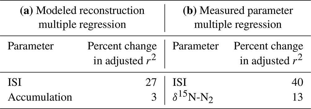
The regression using only measured parameters incorporated δ¹⁵N-N₂ instead of using the modeled accumulation rate. Results are listed in Table 3. We find a maximum adjusted r²= 0.62 (p < 0.0001). Both the modeled and measured parameter multiple regressions compare well (Fig. 9).

For both the modeled and measured regression models, addition of other climate variables increased the goodness of fit. Adding temperature and Δage to the modeled multiple regression increased the r² to 0.72. Adding δ¹⁵N-N₂ and δ¹⁸O_ice to the measured parameter multiple regression increased the r² to 0.69. While adding these parameters increased the goodness of fit of the models, suggesting that they do record phenomena important to controlling TAC, the other climate parameters are also highly correlated between themselves, which makes the interpretation of the regression parameters difficult (Gregorich et al., 2021).

Large misfits between the multiple-regression solution and measured TAC seem to occur during times when the climate is rapidly changing. An interesting feature of this analysis is that if the derivative of Δage (dΔage $/$ dt) is added to the multiple regression, it seems to explain more of the variability observed in the TAC record. A comparison between a regression that includes dΔage $/$ dt and a regression that does not is shown in Fig. 9. Specifically, dΔage $/$ dt seems to correlate well with the magnitude of TAC change that occurs at 2600 years as well as the large variations that occur between 45 ka and the oldest part of the record. A regression analysis that includes dΔage $/$ dt and the measured parameters (ISI, δ¹⁵N-N₂, δ¹⁸O_ice, and Δage) gives an adjusted r² of 0.77 (p < 0.0001), meaning that the dΔage $/$ dt and its interactions describe about 8 % of the measured data multiple-regression solution. Adding dΔage $/$ dt to the modeled reconstruction multiple regression increases the r² adjusted by 4 %.

A possible explanation for why dΔage $/$ dt explains this extra variation is that Δage responds to changing climate conditions, and times when Δage is changing rapidly (large dΔage $/$ dt) correspond to large changes in temperature and accumulation rate not tracked adequately with other variables. We specifically observe this at D–O 12 and 13. This agreement between large dΔage $/$ dt and rapid climate changes again points to a mechanism in the firn column that responds to transient accumulation changes. Following the reasoning of Eicher et al. (2016), times of large changes in accumulation may not allow the firn to form spherical bubbles, creating less pore space, and therefore lower TAC values.

An observation that is not explained by the multiple regression is the apparent lack of TAC variability from around 25 to 42 ka. This section of the record seems to stop responding to millennial-scale forcing. In fact, our multiple regression predicts millennial-scale changes during this time that are not realized in the TAC record, most notably a large predicted change around 32 ka that is not reflected in TAC. A possible explanation for the lack of variation could be that the effect of accumulation rate on TAC is inhibited when ISI is at a minimum. This inhibition of accumulation effects on grain size could be due to ISI dominating the grain metamorphism mechanism during that period. However, more detailed studies including high-resolution TAC through multiple orbital cycles would be needed to address this question.

4 Conclusion

We present a high-resolution total air content record from the SPC14 ice core covering the last 54 kyr. The implications of the analysis of the SPC14 TAC record are twofold. First, this study strongly confirms previous research on Greenland (NGRIP and GRIP) ice cores as well as Antarctic ice cores (EDC) that low-frequency variations in TAC depend on local summer insolation. Importantly, the high correlation with integrated summer insolation (ISI) corroborates the potential to orbitally tune ice age scales using TAC. Second, because the SPC14 ice core was drilled at a location with relatively small expected elevation changes over the course of the ice core history, it provides a good location to study controls on TAC outside the influence of elevation changes. Our results suggest that temperature, accumulation rate, and other firn column properties interact together to affect TAC and provide important context for developing paleoelevation proxies in cores that may have experienced large elevation changes.

We propose that a common mechanism, grain size metamorphism in the top few meters of the firn, can explain both orbital- and millennial-scale timescales of TAC variations in the SPC14 ice core. Although our data are consistent with an orbital-scale impact of ISI on TAC (and an accumulation-driven millennial component), further work is needed. Future directions should include the following:

1. The first is high-resolution sampling of TAC in multiple ice cores. High-resolution data are required to resolve all millennial-scale features in TAC. These features need to be accounted for before applications like paleoelevation constraints are useful. Data should be collected for both Northern Hemisphere and Southern Hemisphere ice cores, and at a variety of accumulation rate regimes.

2. The second is further understanding of links between δ¹⁵N-N₂, Δage, and TAC in ice cores. Accumulation rate can influence δ¹⁵N-N₂ and Δage depending on climate and therefore influence TAC differently at different sites. High-resolution sampling of δ¹⁵N-N₂ in ice cores (and model-independent Δage determinations) could be used in future work to corroborate findings from the SPC14 ice core. Additionally, TAC sampling at locations with well-known accumulation rate histories will provide further constraints.

3. The third is comparison of TAC in regions that have stable elevation histories to regions with unstable elevation histories. Ice cores targeted in coastal regions with hypothesized unstable elevation histories, such as in Western Antarctica, should be targeted for future TAC research.