The evolution of isolated cavities and hydraulic connection at the glacier bed – Part 2: A dynamic viscoelastic model

Many large-scale subglacial drainage models implicitly or explicitly assume that the distributed part of the drainage system consists of subglacial cavities. Few of these models, however, consider the possibility of hydraulic disconnection, where cavities exist but are not numerous or large enough to be pervasively connected with one another so that water can flow. Here I use a process-scale model for subglacial cavities to explore their evolution, focusing on the dynamics of connections that are made between cavities. The model uses a viscoelastic representation of ice and computes the pressure gradients that are necessary to move water around basal cavities as they grow or shrink. The latter model component sets the work here apart from previous studies of subglacial cavities and permits the model to represent the behaviour of isolated cavities as well as of uncavitated parts of the bed at low normal stress. I show that connections between cavities are made dynamically when the cavitation ratio (the fraction of the bed occupied by cavities) reaches a critical value due to decreases in effective pressure. I also show that existing simple models for cavitation ratio and for water sheet thickness (defined as mean water depth) fail to even qualitatively capture the behaviour predicted by the present model.

1 Introduction

Much of the interest in subglacial drainage is motivated by the effect of pressurized subglacial water on glacier sliding (Iken and Bindschadler, 1986): basal friction is reduced when basal water pressure is high or, more precisely, when basal effective pressure is low. The relationship between effective pressure and basal friction is called the basal friction law: a parameterization that computes mean basal drag as a function of basal effective pressure, sliding velocity, and possibly other variables that can be computed by a large-scale model (such as mean cavity size; see e.g. Hewitt, 2013, and Gilbert et al., 2022). First-principles derivations of friction laws (e.g. Weertman, 1957; Nye, 1969; Kamb, 1970; Fowler, 1981, 1986; Schoof, 2005; Gagliardini et al., 2007; Helanow et al., 2020, 2021) average stresses over a local process scale, such as that involved in the ploughing of clasts through till or the flow of ice over bed obstacles, to compute mean drag at the glacier bed.

The basal effective pressure that appears in the friction law is likewise defined as a local spatial average of the difference between local normal stress at the bed and basal water pressure. At the local process scale, actual normal stresses are heterogeneous but have a well-defined average that is generally close to local ice overburden. By contrast, basal water pressure is generally not assumed to be heterogeneous in the friction law. A spatially smoothly varying basal water pressure will result if there is a pervasive, connected subglacial drainage system that causes pressure differences to equilibrate rapidly.

A growing body of observational evidence, however, suggests that hydraulic isolation of significant parts of glacier beds is a common phenomenon, even during the summer melt season. Moreover, different parts of the glacier bed can switch back and forth between being connected and isolated (Fudge et al., 2008; Andrews et al., 2014; Rada and Schoof, 2018). While not included in most of the current generation of widely used subglacial drainage models (Werder et al., 2013; Sommers et al., 2018), there have been some recent attempts to account for hydraulic isolation (Hoffman et al., 2016; Rada and Schoof, 2018). In the framework of modern “distributed” drainage models, dynamic changes in connectivity have to be formulated using the primary model variables, usually effective pressure N and a mean ice–bed gap width (or “water sheet thickness”) $\overline{h}$. The model of Rada and Schoof (2018) uses a discrete network formulation, but its distributed equivalent is a distributed water model (Hewitt, 2011, 2013; Schoof et al., 2012; Werder et al., 2013) in which hydraulic connection is established if sheet thickness $\overline{h}$ exceeds a threshold h_c: that is, a finite water flux through the sheet occurs if

$$\begin{array}{}\text{(1)}& \overline{h}>h_{\mathrm{c}},\end{array}$$

and $\overline{h}$ is usually assumed to evolve according to a model of the form (Hewitt, 2011; Schoof et al., 2012)

$$\begin{array}{}\text{(2)}& {\displaystyle \frac{\partial \overline{h}}{\partial t}}=v_{\mathrm{o}}(\overline{h},u_{\mathrm{b}})-v_{\mathrm{c}}(\overline{h},N).\end{array}$$

Here, u_b is sliding velocity and v_o represents opening of the water sheet due to sliding over bed roughness, while v_c is a creep closure term. (Note that most drainage models dispense with the overbar on $\overline{h}$; I retain it here because I reserve h for the local ice–bed gap width later.)

The justification for such a treatment of hydraulic connection is that small cavities can exist in the lee of bed bumps without being sufficiently connected to each other to allow water flow, as in a percolation problem (Hammersley and Welsh, 1980). While appealing, this simple treatment has not been tested against a process-scale model of subglacial cavity formation. In fact, existing models of cavity formation (Fowler, 1986; Schoof, 2005; Gagliardini et al., 2007; Helanow et al., 2020, 2021; Stubblefield et al., 2021; de Diego et al., 2022, 2023) generally assume that the underlying bed itself is highly permeable and provides easy access for water to be injected into any part of the bed where normal stress in the ice has dropped to the water pressure in an ambient (but not otherwise modelled) drainage system.

The present paper is part of an effort to dispense with that assumption of a perfectly permeable bed and instead study how cavities can expand dynamically along the ice–bed interface from an access point or set of access points where water is injected through the bed at prescribed pressure by an ambient drainage system. In a companion paper (Schoof, 2023), henceforth referred to as Part 1, I have used a modification of existing steady-state cavity models in two dimensions (that is, with only one horizontal dimension) to study cavity expansion under quasi-steady conditions. That is, Part 1 assumes an ambient drainage system with a prescribed effective pressure N that varies slowly enough in time for the cavity roof to always be in a steady state.

Based on that assumption, Part 1 shows that connections between the ambient drainage system and previously uncavitated parts of the bed are made in a quasi-steady state at a set of critical effective pressures. The system of cavities also exhibits hysteresis. If cavity enlargement past a bed protrusion on its downstream side has occurred previously and cavity size has shrunk subsequently due to an increase in ambient effective pressure, then reconnection to the now isolated pre-existing cavities happens at a different set of higher effective pressure: reconnecting to an existing downstream cavity is easier than creating that downstream cavity by enlarging the upstream cavity past the bed protrusion separating the two.

In a time-dependent system, cavity connections are likely to be more complicated than the quasi-steady model suggests. To study dynamic cavity connections, I complement the work in Part 1 with a generalized dynamic model. Ice is treated as viscoelastic to account for the possibility that cavity expansion could be very rapid and occur on timescales that are short compared with the Maxwell time of ice. In addition, I explicitly account for the water pressure gradients that are necessary to move water around a cavity, in particular, into any ice–bed gaps that are newly created when rapid cavity enlargements occur. By using a mass conservation model for water with a water flux that vanishes when the ice–bed gap size goes to zero, the dynamic model not only allows the process of cavity expansion to be captured dynamically, but also allows for the dynamic evolution of isolated cavities.

The generalized model in the present paper is formulated in three dimensions. In principle, this avoids another of the limitations of the work in Part 1. Because the MATLAB code I have written is not suitable for full parallelization, I have not been able to run the model in three dimensions except for very coarse meshes, leaving an obvious avenue for future research.

The paper is structured as follows: in Sect. 2.1, I formulate a basic model for viscoelastic ice flow over a rigid bed, with a dynamically evolving water layer separating ice and bed. The model is reduced using the assumption of small bed slopes in Sect. 2.2, while a numerical method for the reduced model is described in Sect. 2.3. Steady-state numerical solutions of the dynamic model are compared with solutions of the simpler viscous steady-state model in Part 1 in Sect. 3.1. The dynamic approach to steady state is studied in Sect. 3.2, with dynamic cavity connections considered in greater detail in Sect. 3.3. The evolution of overpressurized cavities (in which effective pressure is negative) is described in Sect. 3.4, and the response of isolated cavities to temporal variations in forcing effective pressure is studied in Sect. 3.5. The implication of these results for large-scale drainage models and field observations is discussed in Sect. 4.

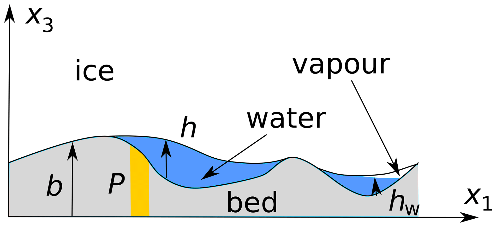
Figure 1 Definitions used in the paper. Beige is used throughout the paper to indicate the connection portions P of the bed. h is used here to denote the ice–bed gap, which will often be equal to water depth h_w, but can differ if water pressure vanishes, and a partially vapour-filled cavity forms. In this figure, the large cavity overlaps with the connected bed portion P: water freely enters or leaves the cavity at a pressure prescribed by the ambient drainage system through P.

2 A viscoelastic dynamic model

2.1 The basic model

The model in Part 1 is based on the approximation of small bed slopes (Nye, 1969; Kamb, 1970; Fowler, 1981). I will eventually return to that small-slope approximation but first develop a more general three-dimensional formulation. I use a Cartesian coordinate system $(x_{\mathrm{1}},x_{\mathrm{2}},x_{\mathrm{3}})$ with the x₃ axis oriented perpendicularly to the mean glacier bed and x₁ in the mean downslope direction (Fig. 1), and I denote time by t. The rheology of ice is treated here as an elastically compressible upper-convected Maxwell fluid, in which stress σ_ij is related to strain rate D_ij as (e.g. Bird, 1976)

$$\begin{array}{}\text{(3)}& {\displaystyle \frac{(\mathrm{1}+\mathit{\nu }){\mathit{\delta }}_{ik}{\mathit{\delta }}_{jl}-\mathit{\nu }{\mathit{\delta }}_{ij}{\mathit{\delta }}_{kl}}{E}}{\stackrel{▿}{\mathit{\sigma }}}_{kl}+{\displaystyle \frac{\mathrm{1}}{\mathrm{2}\mathit{\eta }}}\left({\mathit{\sigma }}_{ij}-{\displaystyle \frac{\mathrm{1}}{\mathrm{3}}}{\mathit{\sigma }}_{kk}{\mathit{\delta }}_{ij}\right)=D_{ij},\end{array}$$

where the superscript ▿ denotes the usual upper-convected derivative

$$\begin{array}{}\text{(4)}& {\stackrel{▿}{\mathit{\sigma }}}_{ij}={\displaystyle \frac{\partial {\mathit{\sigma }}_{ij}}{\partial t}}+u_k{\displaystyle \frac{\partial {\mathit{\sigma }}_{ij}}{\partial x_k}}-{\displaystyle \frac{\partial u_i}{\partial x_k}}{\mathit{\sigma }}_{kj}-{\displaystyle \frac{\partial u_j}{\partial x_k}}{\mathit{\sigma }}_{ik},\end{array}$$

and $(u_{\mathrm{1}},u_{\mathrm{2}},u_{\mathrm{3}})$ denotes the velocity field. Strain rate is defined in terms of velocity through

$$\begin{array}{}\text{(5)}& D_{ij}={\displaystyle \frac{\mathrm{1}}{\mathrm{2}}}\left({\displaystyle \frac{\partial u_i}{\partial x_j}}+{\displaystyle \frac{\partial u_j}{\partial x_i}}\right).\end{array}$$

Here, E is Young's modulus, ν is Poisson's ratio, η is viscosity, and δ_ij is the Kronecker delta. In response to abrupt changes in stress (with large $\partial {\mathit{\sigma }}_{kl}/\partial t$), the rheology reduces to

$${\displaystyle \frac{(\mathrm{1}+\mathit{\nu }){\mathit{\delta }}_{ik}{\mathit{\delta }}_{jl}-\mathit{\nu }{\mathit{\delta }}_{ij}{\mathit{\delta }}_{kl}}{E}}{\displaystyle \frac{\partial {\mathit{\sigma }}_{kl}}{\partial t}}=D_{ij},$$

as the strain due to the change in stress remains small over such short intervals, and hence the advection terms in the upper-convected derivative are small compared with the time derivative. Integrating over the time interval over which the stress change is imposed, it is then clear that the material behaves temporarily as a linear elastic material subject to a viscous pre-stress. If the change in stress occurs over an interval (t_i,t_f), then the change in stress is related to the corresponding linearized strain as

$$\begin{array}{rl}& {\displaystyle \frac{(\mathrm{1}+\mathit{\nu }){\mathit{\delta }}_{ik}{\mathit{\delta }}_{jl}-\mathit{\nu }{\mathit{\delta }}_{ij}{\mathit{\delta }}_{kl}}{E}}\left[{\mathit{\sigma }}_{ij}(x,t_{\mathrm{f}})-{\mathit{\sigma }}_{ij}(x,t_{\mathrm{i}})\right]\\ & ={\mathit{\epsilon }}_{ij}\left(x\right)=\underset{t_{\mathrm{i}}}{\overset{t_{\mathrm{f}}}{\int }}{D}_{ij}(x,t)\mathrm{d}t.\end{array}$$

Conversely, to emulate Glen's law (Cuffey and Paterson, 2010) over long timescales, when the derivative ${\stackrel{▿}{\mathit{\sigma }}}_{kl}$ becomes negligible, one would put $\mathit{\eta }=B|\mathit{\tau }{|}^{\mathrm{1}-n}/\mathrm{2}$, where n and B are the usual exponent and coefficient in Glen’s law, and τ is the usual second invariant of the deviatoric stress tensor,

$$\mathit{\tau }=\sqrt{({\mathit{\sigma }}_{ij}-{\mathit{\sigma }}_{kk}{\mathit{\delta }}_{ij}/\mathrm{3})({\mathit{\sigma }}_{ij}-{\mathit{\sigma }}_{kk}{\mathit{\delta }}_{ij}/\mathrm{3})/\mathrm{2}}.$$

In this paper, I will continue to focus on a simpler version of the model with constant viscosity as in Part 1.

I assume ice occupies a domain defined by $x_{\mathrm{3}}>b(x_{\mathrm{1}},x_{\mathrm{2}})+h(x_{\mathrm{1}},x_{\mathrm{2}},t)$, where b is a fixed bed elevation and h≥0 is an ice–bed gap thickness that can evolve over time. Here, b is identical to its meaning in Part 1 (as shown in Fig. 1 therein), while the sum of bed elevation and gap thickness b+h is the cavity roof elevation h_C in Part 1. I assume that the domain represents a boundary layer near the base of the glacier (Fowler, 1981). Consequently, I assume as in Part 1 that gravitational body forces contribute negligibly to stress compared with overburden, and conservation of momentum can be written in the form

$$\begin{array}{}\text{(6)}& {\displaystyle \frac{\partial {\mathit{\sigma }}_{ij}}{\partial x_j}}=\mathrm{0},\end{array}$$

ignoring inertial effects. Conservation of mass requires

$$\begin{array}{}\text{(7)}& {\displaystyle \frac{\partial \mathit{\rho }}{\partial t}}+{\displaystyle \frac{\partial \left(\mathit{\rho }{u}_i\right)}{\partial x_i}}=\mathrm{0}.\end{array}$$

In common with typical models in elasticity, this equation can be used a posteriori to compute variations in density due to elastic compression of the material, but it is not necessary to compute the velocity field.

At the lower boundary of the ice, $x_{\mathrm{3}}=b(x_{\mathrm{1}},x_{\mathrm{2}})+h(x_{\mathrm{1}},x_{\mathrm{2}},t)$, I assume that there is free slip regardless of whether the macroscopic ice–bed separation h vanishes or not. In the absence of an ice–bed gap in the model, I assume that interfacial premelting (Dash et al., 1995) still generates a microscopic film that ensures negligible shear stress; this is a standard assumption of basal sliding theory. Denoting by n_i the unit normal to the lower boundary of the ice, this implies

$$\begin{array}{}\text{(8)}& ({\mathit{\delta }}_{ij}-n_{\mathrm{i}}{n}_j){\mathit{\sigma }}_{jk}{n}_k=\mathrm{0}.\end{array}$$

The lower boundary also satisfies a kinematic boundary condition of the form

$$\begin{array}{}\text{(9)}& u_{\mathrm{3}}={\displaystyle \frac{\partial h}{\partial t}}+u_{\mathrm{1}}{\displaystyle \frac{\partial (b+h)}{\partial x_{\mathrm{1}}}}+u_{\mathrm{2}}{\displaystyle \frac{\partial (h+b)}{\partial x_{\mathrm{2}}}},\end{array}$$

where melt is taken to be negligible.

To close the problem, I require one additional boundary condition. I consider two alternatives. First, I consider the standard assumption in dynamic models of subglacial cavity formation, namely that the bed is rigid yet highly permeable, with a prescribed water pressure $p_{\mathrm{w}}^{\mathrm{0}}$ everywhere. That assumption is also part of the steady-state model by Fowler (1986) and Schoof (2005) that I previously generalized in Part 1. Normal stress cannot drop below that water pressure, since water forces its way between ice and bed and opens a gap or cavity. A fully permeable bed gives a boundary condition on normal stress in the following either–or form (Durand et al., 2009; Stubblefield et al., 2021; de Diego et al., 2022, 2023):

$$\begin{array}{}\text{(10a)}& {\displaystyle }-{\mathit{\sigma }}_{ij}{n}_{\mathrm{i}}{n}_j=& {\displaystyle }{p}_{\mathrm{w}}^{\mathrm{0}}& {\displaystyle }\text{if }h>\mathrm{0}\text{ or }\left(h=\mathrm{0}\text{ and }{\displaystyle \frac{\partial h}{\partial t}}>\mathrm{0}\right),\text{(10b)}& {\displaystyle }-{\mathit{\sigma }}_{ij}{n}_{\mathrm{i}}{n}_j\ge & {\displaystyle }{p}_{\mathrm{w}}^{\mathrm{0}}& {\displaystyle }\text{if }h={\displaystyle \frac{\partial h}{\partial t}}=\mathrm{0},\end{array}$$

signifying the possibility that compressive normal stress can exceed water pressure where ice is in contact with the bed, and a gap is not about to form: put more simply, in contact areas, normal velocity is prescribed so long as compressive normal stress exceeds water pressure, or else normal stress is prescribed if the ice is about to detach from the bed, and the inequality constraints serve to determine which boundary condition applies where (see also Stubblefield et al., 2021). By contrast, in areas with an ice–bed gap, normal stress is always prescribed. Also note that the model here is formulated in terms of total Cauchy stress, while Part 1 uses a reduced pressure, from which overburden has been subtracted; I introduce that reduction of stress in the next section.

The boundary conditions above do not permit the formation of hydraulically isolated cavities or of underpressurized contact areas that remain hydraulically isolated as in Part 1. As an alternative to the boundary conditions (10), I therefore consider a bed that is perfectly impermeable except in specific locations at which water from an ambient drainage system can enter or exit the ice–bed gap. As in Part 1, I assume that there is a (typically small) highly permeable portion P of the bed through which water can freely flow while remaining at the pressure of the ambient drainage system. Consequently, the boundary conditions (10) hold on P (or, strictly speaking, at the upper boundary of P, but since I do not model water flow through the bed, I will continue to state conditions “on P”, meaning the interface of the permeable bed with a cavity or the lower boundary of the ice). For the remainder of the bed outside of P, I assume that an active hydraulic system inside the ice–bed gap redistributes water.

Specifically, I assume that there is a water column of evolving height h_w inside the ice–bed gap, constrained by $\mathrm{0}\le h_{\mathrm{w}}\le h$. Assuming negligible deviatoric normal stress in the water column, local force balance demands that water pressure p_w in that water column (not to be confused with the prescribed ambient drainage system pressure $p_{\mathrm{w}}^{\mathrm{0}}$, which generally differs from p_w) is given by normal stress at the bed,

$$\begin{array}{}\text{(11a)}& -{\mathit{\sigma }}_{ij}{n}_{\mathrm{i}}{n}_j=p_{\mathrm{w}}.\end{array}$$

Outside of the permeable portion of the bed, there is no water supply, so p_w is not prescribed a priori, but the water column height satisfies a depth-integrated mass conservation equation of the form

$$\begin{array}{}\text{(11b)}& {\displaystyle \frac{\partial h_{\mathrm{w}}}{\partial t}}+{\mathrm{\nabla }}_h\cdot \mathit{q}=\mathrm{0},\end{array}$$

which should be understood in weak form, permitting mass-conserving shocks where necessary. Here $\mathit{q}=(q_{\mathrm{1}},q_{\mathrm{2}})$ is a two-dimensional flux and ${\mathrm{\nabla }}_h=(\partial /\partial x_{\mathrm{1}},\partial /\partial x_{\mathrm{2}})$ is the corresponding two-dimensional divergence operator. I assume that the ice–bed gap is shallow (an assumption that I formalize in the next section), and I therefore relate the depth-integrated water flux q to water column height h_w and an along-bed gradient in water pressure $p_{\mathrm{w}}(x_{\mathrm{1}},x_{\mathrm{2}},t)$ as

$$\begin{array}{}\text{(11c)}& \mathit{q}=-K\left(h_{\mathrm{w}},\left|{\mathrm{\nabla }}_h{p}_{\mathrm{w}}\right|\right){\mathrm{\nabla }}_h{p}_{\mathrm{w}}+{\displaystyle \frac{\mathrm{1}}{\mathrm{2}}}{\mathit{u}}_h{h}_{\mathrm{w}},\end{array}$$

where ${\mathit{u}}_h=(u_{\mathrm{1}},u_{\mathrm{2}})$ is the horizontal component of velocity at the base of the ice, and K is a two-dimensional “gap permeability”, which I take to be give by the Darcy–Weisbach or Manning–Gauckler power-law formulation (see e.g. Werder et al., 2013), of the generic form

$$\begin{array}{}\text{(11d)}& K(h_{\mathrm{w}},|{\mathrm{\nabla }}_h{p}_{\mathrm{w}}\left|\right)=k_{\mathrm{0}}{h}_{\mathrm{w}}^{\mathit{\alpha }}{\left|{\mathrm{\nabla }}_h{p}_{\mathrm{w}}\right|}^{\mathit{\beta }-\mathrm{1}},\end{array}$$

with α>1, $\mathit{\beta }=\mathrm{1}/\mathrm{2}$, and k₀>0 constant. Note that the above also covers the case of laminar Poiseuille flow if α=3 and β=1. The second term in Eq. (11c) is the small contribution of shear to water flux.

Note that Eq. (11b) ignores the compressibility of water, while ice is allowed to be elastically compressible by Eq. (3), despite the bulk moduli being comparable (Neumaier, 2018). This is standard practice in hydrofracture models, whose validity hinges on the assumption of a shallow water layer: in that case, the displacement of the ice–water boundary that results from compression of the water column is small compared with the displacements that result from compression in the ice, simply because compressive strain in water is comparable to its counterpart in the ice, but the resulting displacement (being an integral over strain) is much smaller than in the ice.

To avoid the negative fluid pressure singularities common to hydrofracture models (Spence et al., 1985; Tsai and Rice, 2010, 2012), I permit a “fluid lag” in the form of a vapour-filled space between water and ice when water pressure drops to zero (or, more strictly, the triple-point pressure of water, which I treat as negligibly small compared with stresses in the ice). This means that fluid depth h_w and ice–bed gap size h are related through one of the following two possibilities:

$$\begin{array}{}\text{(11e)}& {\displaystyle }\text{either }\mathrm{0}\le h_{\mathrm{w}}=& {\displaystyle }h& {\displaystyle }\text{and }{p}_{\mathrm{w}}>\mathrm{0}\text{(11f)}& {\displaystyle }\text{or }\mathrm{0}\le h_{\mathrm{w}}\le & {\displaystyle }h& {\displaystyle }\text{and }{p}_{\mathrm{w}}=\mathrm{0},\end{array}$$

and p_w cannot be negative.

The first possibility, condition (11e), states that there cannot be a vapour-filled gap between ice and water (of thickness $h-h_{\mathrm{w}}>\mathrm{0}$) if fluid pressure is above the triple-point pressure in the sense that ice, water, and vapour cannot then coexist. This is the default state and corresponds to a completely fluid-filled ice–bed gap, as is the case in the canonical picture of subglacial cavities. By the second condition (11f), a water-filled gap is possible but need not exist at the triple-point pressure; given the substantial overburden pressure, this is only likely to be reached near the tips of cavities that are in the process of expanding rapidly (e.g. Tsai and Rice, 2010).

As far-field boundary conditions, I consider prescribed normal and shear stress in the form

$$\begin{array}{}\text{(12)}& -{\mathit{\sigma }}_{\mathrm{33}}\to p_i,{\mathit{\sigma }}_{\mathrm{13}}\to {\mathit{\tau }}_{\mathrm{b}},{\mathit{\sigma }}_{\mathrm{23}}\to \mathrm{0}\end{array}$$

as x₃→∞, where p_i is overburden and τ_b is the usual “basal shear stress” of the theory of basal sliding (Fowler, 1981). In addition, I assume the domain is laterally periodic, with period a in both horizontal directions.

The basal boundary conditions for the classical cavitation problem with a permeable bed consist of Eqs. (8), (9), and the complementarity condition (10). The stress and normal velocity conditions (8) and (10) are sufficient to close the force balance problem (6) (see de Diego et al., 2022, 2023; Stubblefield et al., 2021, for the equivalent purely viscous problem), while the kinematic boundary condition (9) serves to determine the gap width variable h that appears in the contact conditions (10).

By contrast, the equivalent set of boundary conditions for an impermeable bed given above introduces local fluid pressure p_w and fluid depth h_w as variables defined at the boundary, in addition to the gap width h. A simple counting argument shows that Eqs. (8) and (9) combined with Eqs. (11b)–(11f) close the problem: the force balance relation in Eq. (6) requires three boundary conditions, which are supplied by Eqs. (8) and (11a). The fluid pressure p_w featured in Eq. (11a) is determined through the mass conservation problem in Eq. (11b)–(11c). The latter constitute a single equation in fluid depth h_w and pressure p_w, where h_w and gap width are determined through the kinematic boundary condition (9) and whichever one of the two conditions (11e)–(11f) applies, leading to a total of three equations to specify the three variables p_w, h_w, and h.

The counting argument of the previous paragraph is of course simplistic: the determination of p_w, h_w, and h couples back to the force balance problem through the velocity components in the kinematic boundary condition. Also note that isolated cavities (the object of our study) are only present if the gap width h is either zero or extremely small between those cavities and the permeable bed portion P. The formulation above incorporates such regions provided the permeability K vanishes when fluid depth h_w does (as it must where the gap vanishes, since h_w≤h). In the interior of a region where the ice–bed gap vanishes (that is, where ice is in contact with the bed), water flux vanishes and hence $\partial h_{\mathrm{w}}/\partial t=\mathrm{0}$ from Eq. (11b). Note that, since there is no water column present in that case, the variable p_w does not represent an actual fluid pressure in such regions but simply equals the compressive normal stress.

From the gap width relations (11e)–(11f), there are then two possibilities in the interior of regions where h_w=0: either h remains at zero and the kinematic boundary condition (9) reduces to a condition of vanishing normal velocity, so $u_{\mathrm{3}}=u_{\mathrm{1}}\partial b/\partial x_{\mathrm{1}}+u_{\mathrm{2}}\partial b/\partial x_{\mathrm{2}}$ and ice remains in contact with the bed, or, alternatively normal stress drops to the triple-point pressure and a vapour-filled cavity forms. The combination of Eqs. (8), (9), and (11b)–(11f) can therefore describe not only the physics of a water layer separating ice and bed, but also the physics of ice–bed contact areas as required.

In practice, only very small pressure gradients should be required in order to move water fast enough to fill the ice–bed gap as the latter evolves due to ice flow. That situation corresponds to the limit of a large gap permeability K (or better, of large k₀): the flux relation (11c) then simply serves at leading order to impose a spatially uniform water pressure in each basal cavity, as is also the case for the classical cavity model using the permeable-bed boundary conditions (10). In that case, shear in the water column also plays an insignificant role, and I retain the second term ${\mathit{u}}_h{h}_{\mathrm{w}}/\mathrm{2}$ in the definition of flux in Eq. (11c) here simply to make the switch to the moving coordinate frame employed in Sect. 2.3 more self-consistent (since an advective term will automatically appear under the change to a moving frame).

2.2 Shallow bed topography

Significant simplifications can be obtained by considering flow over “shallow” bed roughness, meaning a bed b(x₁,x₂) with small slopes (see e.g. Nye, 1969; Kamb, 1970; Fowler, 1986; Schoof, 2005). To obtain a simplified model systematically, I sketch the required non-dimensionalization here, building primarily on the seminal work of Fowler (1981). Defining a horizontal length scale [x] for typical bed roughness wavelengths and a scale [b] for the amplitude of roughness leads to a slope scale

$$\begin{array}{}\text{(13)}& \mathit{\epsilon }={\displaystyle \frac{\left[b\right]}{\left[x\right]}},\end{array}$$

and the basis of the approximations that follow will be ε≪1. With a sliding velocity scale u_b for motion parallel to the bed, I can define a scale for velocity variations induced by deformation around bed topography as [u]=εu_b and a corresponding (viscous) stress scale as $\left[\mathit{\sigma }\right]=\mathit{\eta }\left[u\right]/\left[x\right]$. A natural choice of timescale is the advective $\left[t\right]=\left[x\right]/u_{\mathrm{b}}$, and I assume that there is a density scale [ρ] given by the density of ice subject to zero stress.

With these scales in hand, I can define dimensionless variables as

$$\begin{array}{}\text{(14)}& \begin{array}{rl}& (x_{\mathrm{1}},x_{\mathrm{2}},x_{\mathrm{3}})=\left[x\right](x_{\mathrm{1}}^{*},x_{\mathrm{2}}^{*},x_{\mathrm{3}}^{*}),\\ & (u_{\mathrm{1}},u_{\mathrm{2}},u_{\mathrm{3}})=u_{\mathrm{b}}(\overline{u},\overline{v},\mathrm{0})+\left[u\right](u_{\mathrm{1}}^{*},u_{\mathrm{2}}^{*},u_{\mathrm{3}}^{*}),\\ & p_{\mathrm{w}}=p_i+\left[\mathit{\sigma }\right]p_n^{*},{\mathit{\sigma }}_{ij}=\left\{\begin{array}{cc}-p_i+\left[\mathit{\sigma }\right]{\mathit{\sigma }}_{\mathrm{33}}^{*}& \text{if }i=j=\mathrm{3},\\ \left[\mathit{\sigma }\right]{\mathit{\sigma }}_{ij}^{*}& \text{otherwise},\end{array}\right.\\ & \mathit{\rho }=\left[\mathit{\rho }\right]{\mathit{\rho }}^{*}\\ & b=\left[b\right]b^{*},h=\left[b\right]h^{*},h_{\mathrm{w}}=\left[h\right]h_{\mathrm{w}}^{*}.\end{array}\end{array}$$

In addition, I obtain the following dimensionless parameters

$$\begin{array}{}\text{(15)}& \begin{array}{rl}\mathit{\kappa }& ={\displaystyle \frac{\left[t\right]K\left(\right[b],[\mathit{\sigma }]/[x\left]\right)\left[\mathit{\sigma }\right]}{\left[b\right][x{]}^{\mathrm{2}}}}={\displaystyle \frac{k_{\mathrm{0}}\left[t\right]\left[b{]}^{\mathit{\alpha }-\mathrm{1}}\right[\mathit{\sigma }{]}^{\mathrm{1}/\mathrm{2}}}{[x{]}^{\mathrm{3}/\mathrm{2}}}},\\ {\mathit{\tau }}_{\mathrm{M}}& ={\displaystyle \frac{\mathrm{2}\mathit{\eta }}{E\left[t\right]}},{\mathit{\tau }}_{\mathrm{b}}^{*}={\displaystyle \frac{{\mathit{\tau }}_{\mathrm{b}}}{\mathit{\epsilon }\left[\mathit{\sigma }\right]}},N^{*}={\displaystyle \frac{p_i-p_{\mathrm{w}}^{\mathrm{0}}}{\left[\mathit{\sigma }\right]}},{\mathrm{\Sigma }}_{\mathrm{0}}={\displaystyle \frac{p_i}{\left[\mathit{\sigma }\right]}}.\end{array}\end{array}$$

Here τ_M is a dimensionless Maxwell time, κ is a dimensionless ice–bed gap permeability, and ${\mathit{\tau }}_{\mathrm{b}}^{*}$ is a dimensionless basal shear stress, while N^* is the usual (but scaled) effective pressure defined as the difference between overburden and the water pressure in the “ambient” drainage system to which the bed is connected in the permeable regions P. Note that $p_n^{*}$ is a reduced normal stress (equivalent to the Lagrange multiplier λ in de Diego et al., 2022), defined as the difference between local normal stress p_w (the latter only being equal to water pressure where water is present between ice and bed as discussed in Sect. 2.1) and overburden. Where water is present, $p_n^{*}$ is then the negative of the effective pressure defined in terms of local rather than ambient drainage system water pressure.

Going forward, I will assume that ε≪1. In addition, the Maxwell time τ_M≪1 is short (so that the ice for the most part behaves as a viscous material, as is the case in existing models for subglacial cavity formation) and permeability κ≫1 is large (so that water pressure in a connected portion of the ice–bed gap rapidly equalizes, as is also assumed in existing models, which do not attempt to model the dynamic redistribution of water inside cavities). However, unlike ε, both τ_M and κ will be explicitly retained in the model to capture rapid changes in ice–bed gap during cavity connection events.

I omit the asterisk decorations immediately for improved readability. To an error of O(ε), the model becomes

$$\begin{array}{}\text{(16a)}& {\displaystyle }\begin{array}{rl}& {\mathit{\tau }}_{\mathrm{M}}\left[(\mathrm{1}-\mathit{\nu }){\mathit{\delta }}_{ik}{\mathit{\delta }}_{jl}-\mathit{\nu }{\mathit{\delta }}_{ij}{\mathit{\delta }}_{kl}\right]\left({\displaystyle \frac{\partial {\mathit{\sigma }}_{kl}}{\partial t}}+\overline{u}{\displaystyle \frac{\partial {\mathit{\sigma }}_{kl}}{\partial x_{\mathrm{1}}}}+\overline{v}{\displaystyle \frac{\partial {\mathit{\sigma }}_{kl}}{\partial x_{\mathrm{2}}}}\right)\\ & +{\mathit{\sigma }}_{ij}={\displaystyle \frac{\partial u_i}{\partial x_j}}+{\displaystyle \frac{\partial u_j}{\partial x_i}}\text{ for }{x}_{\mathrm{3}}>\mathrm{0},\end{array}\text{(16b)}& {\displaystyle \frac{\partial \mathit{\rho }}{\partial t}}+\overline{u}{\displaystyle \frac{\partial \mathit{\rho }}{\partial x_{\mathrm{1}}}}+\overline{v}{\displaystyle \frac{\partial \mathit{\rho }}{\partial x_{\mathrm{2}}}}=\mathrm{0}\text{ for }{x}_{\mathrm{3}}>\mathrm{0},\text{(16c)}& {\displaystyle \frac{\partial {\mathit{\sigma }}_{ij}}{\partial x_j}}=\mathrm{0}\text{ for }{x}_{\mathrm{3}}>\mathrm{0},\text{(16d)}& {\displaystyle }{\mathit{\sigma }}_{i\mathrm{3}}=\mathrm{0}\text{ for }i=\mathrm{1},\mathrm{2}\text{ at }{x}_{\mathrm{3}}=\mathrm{0},\text{(16e)}& {\displaystyle }-{\mathit{\sigma }}_{\mathrm{33}}=p_n,\text{ at }{x}_{\mathrm{3}}=\mathrm{0},\text{(16f)}& {\displaystyle \frac{\partial h}{\partial t}}+\overline{u}{\displaystyle \frac{\partial (b+h)}{\partial x_{\mathrm{1}}}}+\overline{v}{\displaystyle \frac{\partial (h+b)}{\partial x_{\mathrm{2}}}}=u_{\mathrm{3}}\text{ at }{x}_{\mathrm{3}}=\mathrm{0},\end{array}$$

with two possible closures. The first, which I refer to as a permeable bed, puts

$$\begin{array}{}\text{(17a)}& {\displaystyle }{p}_n=& {\displaystyle }-N& {\displaystyle }\text{if }h>\mathrm{0}\text{ or }\left(h=\mathrm{0}\text{ and }{\displaystyle \frac{\partial h}{\partial t}}>\mathrm{0}\right)\text{(17b)}& {\displaystyle }{p}_n\ge & {\displaystyle }-N& {\displaystyle }\text{if }h={\displaystyle \frac{\partial h}{\partial t}}=\mathrm{0}\end{array}$$

at x₃=0. The second, which I refer to as an impermeable bed, imposes the boundary conditions (17) only for points $(x_{\mathrm{1}},x_{\mathrm{2}})\in P$ (that is, for points that lie in a part of the bed to which the ambient drainage system has access). Flow of water occurs only through the ice–bed gap otherwise, satisfying

$$\begin{array}{}\text{(18a)}& {\displaystyle \frac{\partial h_{\mathrm{w}}}{\partial t}}+{\mathrm{\nabla }}_h\cdot \mathit{q}=\mathrm{0},\text{(18b)}& {\displaystyle }\mathit{q}=-\mathit{\kappa }{h}_{\mathrm{w}}^{\mathit{\alpha }}{\left|{\mathrm{\nabla }}_h{p}_n\right|}^{-\mathrm{1}/\mathrm{2}}{\mathrm{\nabla }}_h{p}_n+{\displaystyle \frac{\mathrm{1}}{\mathrm{2}}}{h}_{\mathrm{w}}\overline{u},\text{(18c)}& {\displaystyle }{h}_{\mathrm{w}}=h\text{ if }{p}_n>-{\mathrm{\Sigma }}_{\mathrm{0}},\text{(18d)}& {\displaystyle }{h}_{\mathrm{w}}\le h\text{ if }{p}_n=-{\mathrm{\Sigma }}_{\mathrm{0}}.\end{array}$$

with $p_n\ge -{\mathrm{\Sigma }}_{\mathrm{0}}$ and $\overline{\mathit{u}}=(\overline{u},\overline{v})$. The far-field boundary conditions are

$$\begin{array}{}\text{(19)}& {\mathit{\sigma }}_{i\mathrm{3}}\to \mathrm{0}\text{for }i=\mathrm{1},\mathrm{2},\mathrm{3}\text{ as }{x}_{\mathrm{3}}\to \mathrm{\infty }.\end{array}$$

Note that the condition σ₁₃→0 imposed here does not conflict with the alternative condition u₁→0 used, for instance, in Schoof (2005): in the purely viscous model in the latter paper, σ₁₃ behaves as $\partial u_{\mathrm{1}}/\partial x_{\mathrm{3}}$ in our present notation, and σ₁₃→0 implies u₁→ constant. Setting that constant to zero simply removes the indeterminacy of u₁ in the model above (consisting of Eqs. 16–19), which arises because the latter remains invariant under adding a constant to u₁: that indeterminacy needs to be resolved by going to higher order but does not affect the leading-order sliding velocity since u₁ is a small correction to the sliding velocity $\overline{u}$ since $\left[u\right]/u_{\mathrm{b}}=\mathit{\epsilon }\ll \mathrm{1}$. The total velocity is u_b+εu₁ and therefore remains equal to u_b at leading order regardless of what finite value u₁ approaches as x₃→∞.

As in other models of basal sliding with small-slope bed roughness (Nye, 1969; Kamb, 1970; Fowler, 1981, 1986; Schoof, 2005), the basal shear stress τ_b is a higher-order correction to the basal stress field: a relationship between the applied shear stress (τ_b,0) and the sliding velocity $(\overline{u},\overline{v})$ (that is, a friction law) can be computed by considering overall force balance at first order in ε. Doing so leads to the following integral constraints (Fowler, 1981):

$$\begin{array}{}\text{(20)}& \begin{array}{rl}{\mathit{\tau }}_{\mathrm{b}}& =-{\displaystyle \frac{\mathrm{1}}{a^{\mathrm{2}}}}\underset{\mathrm{0}}{\overset{a}{\int }}\underset{\mathrm{0}}{\overset{a}{\int }}{\mathit{\sigma }}_{\mathrm{33}}{\displaystyle \frac{\partial (h+b)}{\partial x_{\mathrm{1}}}}\mathrm{d}y\mathrm{d}x,\\ \mathrm{0}& ={\displaystyle \frac{\mathrm{1}}{a^{\mathrm{2}}}}\underset{\mathrm{0}}{\overset{a}{\int }}\underset{\mathrm{0}}{\overset{a}{\int }}{\mathit{\sigma }}_{\mathrm{33}}{\displaystyle \frac{\partial (h+b)}{\partial x_{\mathrm{2}}}}\mathrm{d}y\mathrm{d}x,\end{array}\end{array}$$

where a is the scaled period of the bed. While this is the main objective of many treatments of basal cavitation, my main goal here is to understand the evolution of basal connectivity instead, and I forego the computation of basal drag as a function of sliding velocity, simply imposing a constant sliding velocity: to that end, I also assume that sliding only occurs in the x₁ direction and put $\overline{v}=\mathrm{0}$.

At first sight, this may not seem all that different from the original model of Sect. 2.1. From a computational perspective, major advantages of the reduced model arise from the linearization of the upper-convective derivative into a greatly simplified material derivative in Eq. (16a): effectively, the effect of the small-slope approximation alone is similar to the usual small-strain approximation that can be obtained when explicitly taking the limit of a small Maxwell time. In addition, the small-slope approximation reduces the free boundary problem for the lower boundary of the ice into a problem posed on a fixed domain x₃>0, in which the type of boundary condition that applies at any given part of the boundary must be determined as part of the solution through the inequality constraints in the boundary conditions (17) or (18).

2.3 Numerical method

Computationally, the problem defined in the previous section is well-suited to solution by mixed finite elements in order to handle both the viscoelastic rheology and the inequality-constrained boundary conditions as described in de Diego et al. (2022, 2023). (There is a technical difference here in the sense that the latter authors use mixed finite elements in velocity, pressure, and normal stress at the bed, whereas the compressible problem considered here naturally calls for mixed finite elements in velocity and the full Cauchy stress tensor; the key to handling the boundary conditions is the use of mixed elements for normal stress at the bed.) Unlike these previous studies, an in-depth analysis of the numerical algorithm is not my goal here, in large part due to the complications introduced by the dynamic drainage model (18a). Instead, I hope to spur interest in the problem and development of more sophisticated approaches by showing results using the simplest approach that appears capable of discretizing and solving the model as stated.

I use a coordinate frame moving at the sliding velocity $(\overline{u},\mathrm{0})$ to eliminate the advection terms in Eq. (16a) and (16f) and use a backward Euler step to semi-discretize in time. The time step is fully implicit except for the use of upwinding in the discretization of the mass balance in Eq. (18a), in which I define the upwind direction based on the direction of ∇_hp_w after the previous time step. At each time step, Eq. (16a) combined with Eq. (16c) then takes the mathematical form of a compressible linear elasticity problem, with velocity taking the place of displacement and “elastic” moduli that differ from the usual E and ε (which would become 1 and ν in dimensionless terms): the effective moduli in fact depend on step size δt as well as τ_M and ν. Instead of applying the far-field boundary conditions (19) at infinity, I apply them at a finite distance D from the bed to ensure a finite domain size. I solve Eqs. (16a) with (16c)–(16e) in weak form using piecewise linear finite elements to discretize the velocity field, piecewise constant elements for stress, and a piecewise linear representation along boundary elements for p_w and h. Although piecewise linear finite elements are appropriate for compressible elastic problems of the type solved at each time step (Kikuchi and Oden, 1988), a more sophisticated choice of basis functions may in fact be preferable here as the long-timescale behaviour of the solution can be expected to mimic an incompressible viscous fluid (e.g. Arnold et al., 1984).

To handle the mass conservation problem (18a), I use a finite-volume discretization with piecewise constant h_w, approximating gradients in p_w on element boundaries by using the same piecewise linear representation of p_w as in the weak form of Eq. (16e). A finite-volume scheme is mass-conserving by construction, which is essential in modelling isolated cavities. I use an upwind scheme for flux q to prevent water depth h_w from becoming spuriously negative where there is net water drainage out of a cell. Doing so requires an upwind direction to be defined. I use the upwind direction defined by the water pressure gradient solved for in the previous time step.

Note that in similar elastic problems solved elsewhere, water can never be completely removed from a pre-existing gap, though it can become arbitrarily thin (Balmforth et al., 2010; Warburton et al., 2020). The distinction between a very thin gap and no gap at all is of little consequence here, since I assume that there is free slip at the base of the ice regardless of whether h_w>0, and the permeability approaches zero as h_w does.

The use of piecewise constant finite volumes for h_w conflicts with the natural discretization of h using piecewise linear finite elements; I handle this by using a finite-volume mesh based on a Voronoi tessellation of the bed that is dual to the Delaney triangulation used for the finite-element mesh, ensuring that nodes on which h and p_w are evaluated as part of the finite-element discretization are also cell centres on which h_w is defined. I then impose the conditions (18d) and (18c) pointwise at these nodes or cell centres.

All inequality constraints that are part of the boundary conditions for either the impermeable or permeable bed case can be written as complementarity problems in discretized form, of the generic form

$$f\left(y_{\mathrm{1}}\right)\ge \mathrm{0},g\left(y_{\mathrm{2}}\right)\ge \mathrm{0},f\left(y_{\mathrm{1}}\right)g\left(y_{\mathrm{2}}\right)=\mathrm{0};$$

take the conditions (18c)–(18d) as an example, where $y_{\mathrm{1}}=h-h_{\mathrm{w}}$, $y_{\mathrm{2}}=p_{\mathrm{w}}+p_i$, and f(y₁)=y₁, g(y₂)=y₂. I reformulate each of these complementarity problems generically in the semi-smooth form (see also de Diego et al., 2022, 2023; Zarrinderakht et al., 2022),

$$min\left(f\right(y_{\mathrm{1}}),g(y_{\mathrm{2}}\left)\right)=\mathrm{0},$$

and use a semi-smooth Newton method to solve for each backward Euler step.

The code is written in MATLAB and uses neither adaptive time stepping (beyond automatic step size reduction when the Newton solver fails to converge to a prescribed tolerance for a given backward Euler step) nor adaptive meshing (although the mesh used is non-uniform, with nodes concentrated near the bed). Both of these features would be desirable future improvements. Although the code is written so it can be used for both two- and three-dimensional domains, the lack of adaptive meshing still leads to a relatively coarse resolution along the bed and restricts any realistic use of the code to two dimensions.

3 Results

In the numerical results reported here, I use the model (16) with a prescribed sliding velocity $\overline{u}=\mathrm{1}$ and $\overline{v}=\mathrm{0}$ in a two-dimensional domain of width a=2π, and I employ the simper notation $(x,z)=(x_{\mathrm{1}},x_{\mathrm{3}})$. I use plane strain conditions, in which u₂=0 and none of the variables depend on x₂, but transverse normal stress σ₂₂ is generally not zero or constant in time. I use the double-humped bed defined by

$$\begin{array}{}\text{(21)}& b\left(x\right)=\sin \left(x\right)+\sin \left(\mathrm{2}x\right),\end{array}$$

which is identical to Eq. (10) of Part 1 with h₀=1 and a=2π and therefore makes the dimensionless parameter N here be the direct equivalent of N^* in Part 1. In addition, I either assume a fully permeable bed so that the constraints (17) hold, or I assume that only part of the bed is permeable, applying the constraints (17) to a subset P of the bed. In that case, I set P to be either a small interval around x_P=1.64 or a small interval around x_P=4.65 (the interval being a single cell or element), while boundary conditions (18) hold across the remainder of the bed. The locations x_P are chosen to be identical to those used in Part 1 and correspond to the locations where cavities form at the highest possible effective pressures N.

I use a finite domain depth D=a, and the finite-element mesh consists of 9419 triangles with 4811 non-uniformly distributed nodes, 178 of which are at the bed and form the cell centres of the finite-volume tessellation of the bed. This degree of resolution was practically the maximum I could achieve in MATLAB with multi-threading on six to eight processors. I use a short Maxwell time ${\mathit{\tau }}_{\mathrm{M}}=\mathrm{1}/\mathrm{50}$ and large permeability κ=70, with the intention of representing a viscous limit for the ice and inviscid behaviour in the water column at O(1) timescales. The dimensionless overburden is set to p_i=10³, and in practice (at the resolution that I am able to achieve), the condition (18d) for generating a partially vapour-filled ice–bed gap was never satisfied in the discretized model.

For the purpose of visualizing results, I focus mostly on several easy-to-identify scalar attributes of the solution and their evolution in time, plotting only selected cavity profiles. I identify cavity end points b_j and c_j as the upstream and downstream end points, respectively, of any finite intervals above a minimum threshold size of $|c_j-b_j|\ge \mathrm{0.15}$, in which gap width h exceeds $h_{\mathit{ϵ}}=\mathrm{5}\times {\mathrm{10}}^{-\mathrm{4}}$ everywhere. Two commonly used measures of cavity size are mean cavity size $\overline{h}$ and cavitation ratio θ (Thøgersen et al., 2019). I compute both of these from the following formulae,

$$\overline{h}\left(t\right)={\displaystyle \frac{\mathrm{1}}{a}}\underset{\mathrm{0}}{\overset{a}{\int }}h(x,t)\mathrm{d}x,\mathit{\theta }\left(t\right)={\displaystyle \frac{\mathrm{1}}{a}}\underset{\mathrm{0}}{\overset{a}{\int }}H\left(h\right(x,t)-h_{\mathit{ϵ}})\mathrm{d}x,$$

where H is the usual Heaviside function. Note that θ is simply the fraction of the bed that is cavitated, since $\mathit{\theta }=a^{-\mathrm{1}}\sum (c_j-b_j)$, the sum being taken over all cavities in one bed period. Both θ and $\overline{h}$ could be used to parameterize cavity geometry in a large-scale subglacial drainage model (the scale of individual cavities being “microscopic” in these models; see Hewitt, 2011; Schoof et al., 2012; Werder et al., 2013),

3.1 Steady states: a test case

The dynamic model of Sect. 2 should agree with the simpler, purely viscous model of Part 1 in the limit of a short Maxwell time τ_M (thus ensuring an absence of elastic effects) and of a large cavity permeability parameter κ (ensuring negligible water pressure gradients except where water layer depth h_w vanishes, or nearly does), provided the solution is also in steady state. To test the numerical solution of the dynamic model, I therefore compare its steady-state results with the results of the model of Part 1 for the same forcing effective pressure N and for the same isolated cavity volumes when these are present (Fig. 2). Note that the problem in Part 1 is solved by an entirely different numerical method from that in Sect. 2.3, providing a robust test.

There is an important qualification to the meaning of “steady state” here: I simply compute a numerical solution of the model (16), subject to Eq. (17) in P and boundary conditions (18) elsewhere, for a long time interval. The numerical method in Sect. 2.3 employs a moving frame, so a steady-state solution of the underlying dynamic model is a travelling wave solution in that moving frame. In practice, the solution retains residual oscillations even for large times t. Provided the contact area is substantially larger than a few finite-volume cells, these residual oscillations are small (Fig. 3), and I interpret them as numerical artefacts resulting from the use of a travelling coordinate frame, combined with the inherent heterogeneity involved in an unstructured mesh (which is also still relatively coarse, with 178 finite-volume cells at the lower domain boundary): an underlying steady-state solution in the original coordinate system becomes a travelling wave solution in the travelling frame used for computation. Any grid effects (small or large) are then bound to be periodic, including those involved in the contact area moving relative to the mesh (which presumably account for uplift and therefore cavity shape).

The solutions of the dynamic model (plotted against the original, as opposed to moving, coordinate x in Fig. 2) are therefore not strictly numerical steady states, but an effectively random instant within that residual oscillation cycle. That said, Fig. 2 shows close agreement between the solution of the dynamic model and the steady-state solution of Part 1, at least for the moderate values of N for which the dynamic model produces a recognizable near-steady state within a reasonable time span. This equally applies for solutions with and without isolated cavities. Note, however, that the isolated cavity volume in Fig. 2c differs from that predicted in Sect. 3 of Part 1. That is unsurprising: the isolated cavity volume computed there by the viscous steady-state model of Part 1 results from a very slow change in N and a cavity configuration that is in a quasi-steady state at all times. To compute the solution in Fig. 2, I instead use an abrupt, finite jump in N to force changes in cavity configuration (see also Fig. 3). At the instant when a cavity becomes isolated, that cavity is generally not in steady state, or at the critical value of N at which steady-state cavities first become isolated, and consequently we cannot expect isolated cavity volume to be the same as that computed in Part 1.

Figure 3 provides a further comparison between results of the dynamic model of the present paper and the steady-state solutions of Part 1 in the form of green lines showing mean cavity depth $\overline{h}$ in panel (a) and grey lines showing cavity end-point positions in panel (b), computed as in Part 1. Panel (a) shows that, for small N and for the time intervals over which N is held steady, there are continued oscillations of non-negligible size, which I discuss further in the next section. These have time-averaged cavity depths $\overline{h}$ that are somewhat smaller than the predicted steady-state results. For larger N, the residual oscillations discussed above are of much smaller amplitude and have time-averaged $\overline{h}$ that agrees closely with the steady-state results, but also remains slightly smaller. This is true except once an isolated cavity forms at t=636: the steady-state results as computed using the method from Part 1 predict a smaller isolated cavity than that which is trapped in the dynamic solution as discussed above. In all cases, cavity end-point positions late in each interval of fixed N agree closely with those predicted by the Part 1 steady-state solver, although upstream cavity end points computed by the dynamic model (shown in red) are systematically located slightly downstream of the locations predicted by Part 1. This may in part occur because cavities are very shallow at their upstream ends, and the post-processing of the dynamic model results uses a threshold value of $h\ge \mathrm{5}\times {\mathrm{10}}^{-\mathrm{4}}$ to identify one of the finite-volume cells at the bed as part of a cavity.

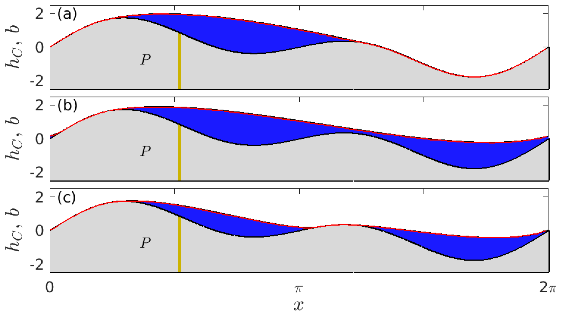
Figure 2 Comparison of steady cavity roof geometry (denoted by b+h for the dynamic model, h_C for the steady viscous model of Part 1) for x_P=1.64. The bed is shown in grey, with the permeable bed portion P in beige. The result for the dynamic model is shown as a blue shaded cavity, and the result of the steady-state model of Part 1 is shown as a red curve. (a) N=1.053 before cavity expansion, (b) N=1.053 after cavity expansion, and (c) N=2.37, with an isolated cavity volume of V₂=1.87 imposed in the model of Part 1, the volume having been computed from the dynamic solution. Note that this cavity volume is different from the value of V₂=1.062 for the isolated cavities that form under quasi-steady conditions for the same bed in Part 1. The two cavity roof shapes are practically indistinguishable in each case.

3.2 Dynamic approach to equilibrium

The purpose of introducing a dynamic model is precisely to study the transient behaviour leading up to the eventual steady state. Figure 3 shows time series of forcing effective pressure N, cavity end positions b_j and c_j, mean cavity size $\overline{h}$, and cavitation ratio θ as the bed is forced with step changes in N through a permeable patch at x_P=1.64.

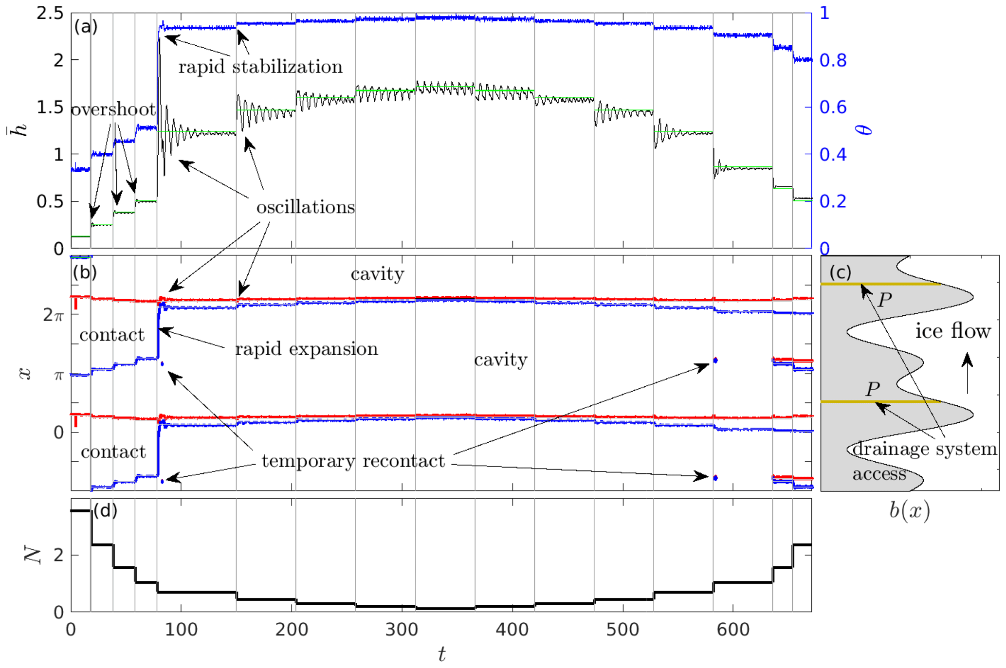
Figure 3 Dynamic cavity evolution under step changes in forcing effective pressure N with P={1.64}. (a) Mean cavity depth $\overline{h}$ (black, left-hand axis) and cavitation ratio θ (blue, right-hand axis) against time t. Green shows the steady-state mean cavity depth computed as in Part 1. (b) Cavity end-point locations at the upstream (red) and downstream (blue) end of cavities against t. Grey shows the steady-state cavity end-point positions as computed in Part 1. (c) The corresponding shape of the bed with the permeable region P in beige. The direction of ice flow (in the positive x direction) is indicated by an arrow; the flipped x and b axes mean that the bed shape is a mirror image of that in Fig. 2. (d) The forcing effective pressure N as a function of time. Grey vertical lines in panels (a)–(b) and (d) indicate abrupt changes in N. The solutions in panels (a)–(c) in Fig. 2 correspond to the solutions here at t=78, t=636, and t=670, respectively.

As expected from Part 1, the steady-state mean cavity size $\overline{h}$ and cavitation ratio θ increase as N is decreased, and the rapid expansion of the cavity after t=78 is irreversible. The dominant feature of the time series is, however, the overshoot in $\overline{h}$ after each step in N occurs: $\overline{h}$ transiently exceeds its new equilibrium value following each decrease in N and conversely drops below its equilibrium value following an increase in N. This overshoot is barely perceptible at the scale shown in Fig. 3 for cases where a significant part of the bed remains uncavitated (with θ close to 0.5, at times prior to t=78) or when there are two separate contact areas (after t=636). The overshoot is much more clearly visible for the latter case in the solutions shown in Fig. 4, where a shorter overall time interval is plotted.

The overshoot becomes large once there is only a single contact area with a cavitation ratio close to unity (between t=78 and t=636 in Fig. 3). In each case, the overshoot is followed by an oscillatory approach to equilibrium. Once again, the nature of the oscillatory approach to equilibrium depends on the extent of cavitation: when there is a single contact area with θ close to unity, the dominant (peak-to-peak) period of oscillation is close to the advective timescale $a/\overline{u}$ for one bed wavelength a, and attenuation to equilibrium is slow, often taking several oscillation periods for the amplitude to halve. The magnitude of the overshoot and subsequent oscillations is largest immediately after contact with the smaller bed protrusion is lost and the cavity expands rapidly after t=78: in fact, the oscillations are large enough for the ice to contact the smaller bed protrusion temporarily as marked in Fig. 3b.

Conversely, if there is limited cavity extent with only the lee of the larger bed protrusion cavitated and θ close to 0.5 (again prior to t=78), or if there are two separate contact areas (after t=636), attenuation is much more rapid, and the dominant peak-to-peak period is approximately half the advection timescale for one bed wavelength. Additional bed contact therefore appears to have a significant damping effect on the oscillations.

The most sustained oscillations occur when there is a single small contact area in each bed period at low effective pressure N (an arguably contrived situation for real glacier beds). Note that the cavitation ratio θ overshoots only slightly (Fig. 3a) and approaches equilibrium rapidly, while cavity height $\overline{h}$ continues to oscillate significantly. Cavitation ratio and ice–bed gap size are therefore not good proxies for each other. Closer inspection of the cavity end-point locations in Fig. 3b for the interval between t=78 and t=636 indicates that the continued oscillations in $\overline{h}$ coincide with in-phase oscillations of both cavity end points. In the absence of comparable oscillations in θ, this implies a back-and-forth motion of the contact area, without significant change in its size. That contact area motion occurs around the top of the prominent bed protrusion at x=0.8. A change in position of the contact area there leads to a significant fractional change in the slope $\partial b/\partial x$ that the ice is incident on (since this location is the maximum of b, where ${\partial }^{\mathrm{2}}b/\partial x^{\mathrm{2}}$ is large and negative). Changes in bed slope in the contact area in turn affect vertical velocities through Eq. (16f) (where the ice–bed gap h vanishes in the contact area).

These variations in vertical velocity are presumably the reason for the significant oscillations in $\overline{h}$: when v₃ is larger, this causes uplift of the cavity roof downstream of the contact area, and that uplifted cavity roof causes the contact point to migrate downstream too, causing the contact area to move over time to a flatter location, thereby reducing the amount of uplift. That in turn causes reduced uplift of the cavity roof, so the contact area moves again to a steeper part of the bed, restarting the cycle (albeit with a smaller amplitude in each cycle). I illustrate the interactions between contact slope angle and growth of the cavity further in Sect. 3.3, in particular in Figs. 8–9, and in video V1 in the Supplement, which shows an animation of the evolving cavity shape corresponding to Fig. 3.

In its simplest form, this mechanism is what happens if one rigid corrugated surface is dragged over another (imagine two pieces of corrugated sheet roofing moving relative to each other); in the present case, the ability of the ice to deform is significant, and the lower surface of the ice does change shape to adapt to the rigid bed underneath, which accounts for the approach to a steady state. It is then perhaps not surprising that low effective pressure N gives rises to the most sustained oscillations: deviatoric stresses in the ice are then small, leading to less rapid deformation of the ice as it moves over the bed, and adjustment to a new steady state is slower than when stresses are larger. This is particularly evident in video V1 in the Supplement.

The generic behaviour shown in Fig. 3 is not unique to either starting with a small cavity and an isolated low-pressure bed region (as is the case before the cavity rapidly expands at t=78) or indeed having only a limited permeable bed patch P. Figure 4 shows a solution for step changes in N with the same bed configuration as in Fig. 3, but with an initial condition that includes an isolated cavity in the lee of the smaller bed protrusion. The oscillatory approach to equilibrium clearly mimics that in Fig. 3, except for the absence of dramatic oscillations following cavity connection (after t=78 in Fig. 3 and after t=40 here): connection with an existing cavity involves relatively small changes in $\overline{h}$ in Fig. 4, so the lack of a large overshoot in Fig. 4 is not surprising.

Figure 5 shows a similar solution for stepwise changes in N, but now with a fully permeable bed. Except for the assumption of a viscoelastic rheology and small bed slopes, this case is analogous to those in Gagliardini et al. (2007), Helanow et al. (2020, 2021), Stubblefield et al. (2021), and de Diego et al. (2022, 2023). Note that viscoelasticity should be mostly irrelevant here, since there are limited changes in the solution that occur over short timescales ∼τ_M, and where significant changes occur that rapidly, they invariably do so immediately after a step change in N. Here, too, we see that $\overline{h}$ overshoots its equilibrium value and decays in an oscillatory manner, though I have not chosen to run each step in N for long enough to see a complete approach to equilibrium. As in the case of an only partially permeable bed, the oscillations in $\overline{h}$ are again much longer-lasting when there is a single contact area per bed wavelength a, and the period of oscillations approximately doubles when contact is lost with the smaller bed protrusion, while the cavitation ratio does not exhibit the same degree of oscillatory behaviour.

While the dynamic behaviour of the fully permeable bed case is similar to the impermeable bed, there are two notable differences. First, as in the case of reconnection of a previously isolated cavity for the impermeable bed case in Fig. 4, drowning of the smaller bed protrusion for the permeable bed does not cause the significant overshoot oscillation that is apparent at t=78 in Fig. 3. Second, the irreversible nature of cavity expansion at that point in time in Fig. 3 is absent for the permeable bed case in Fig. 5, confirming the steady-state results of Part 1.

The cavitation ratio is very close to unity (typically around 0.96–0.) for the long-lasting oscillations at low N identified above (between t=258–420 and t=200–260 in Figs. 3 and 5, respectively). With such a small contact area, only about three to six nodes in the finite-element mesh are in contact with the bed (also note that the numerical method treats a bed cell as either separated from the bed with h>0 or in contact with h=0, and the cavity end-point location therefore jumps in increments of a single cell size, giving the plots of θ and of cavity end-point location against t a non-smooth appearance, while the mean ice–bed separation $\overline{h}$ is much smoother).

A very small number of nodes in contact with the bed raises the question of numerical artefacts. A comprehensive study of mesh size effects is beyond the scope of the work presented here. Due to the limitations of working in a MATLAB coding environment, it is difficult to refine the mesh significantly beyond what is used in the computations reported above. For the case of a fully permeable bed (which typically permits larger time steps), I have been able to refine the mesh to double the number of nodes on the bed for a relatively short computation. A comparison for a shortened version of the computation in Fig. 5 is shown in Fig. 6. While there are differences, these are mostly in the detail: the cavitation ratio time series is significantly smoother for the higher-resolution results (as might be expected), and the oscillations in $\overline{h}$ are also somewhat smoother. There are, however, no dramatic changes of the kind that one might expect for a mesh that is effectively very coarse around the contact area, lending confidence to the conclusion that the sustained oscillations in $\overline{h}$ at low effective pressure are a robust feature of the solution.

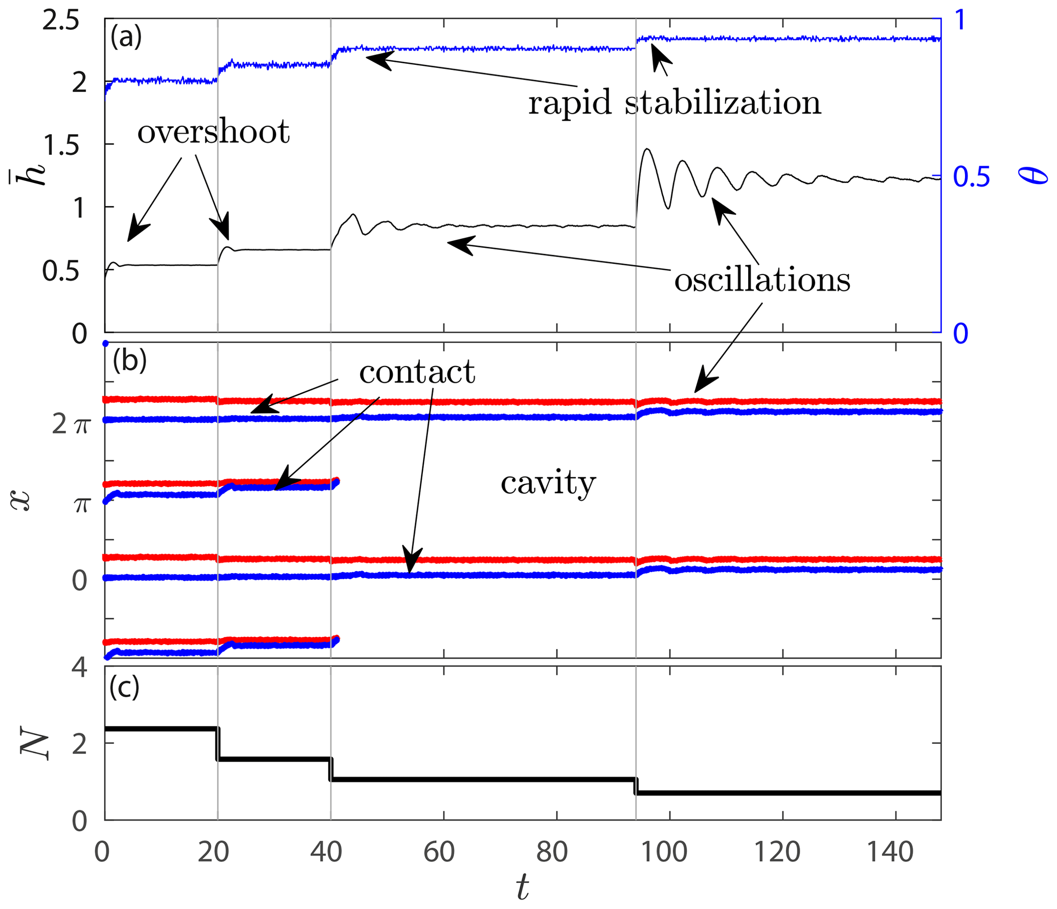
Figure 4 Using the same plotting scheme as in Fig. 3, dynamic cavity evolution under step changes in N with P={1.64}. Here the initial state includes an isolated cavity around x=4.65.

Figure 5 Using the same plotting scheme as in Fig. 3, dynamic cavity evolution under step changes in N with a fully permeable bed, $P=(\mathrm{0},a)$.

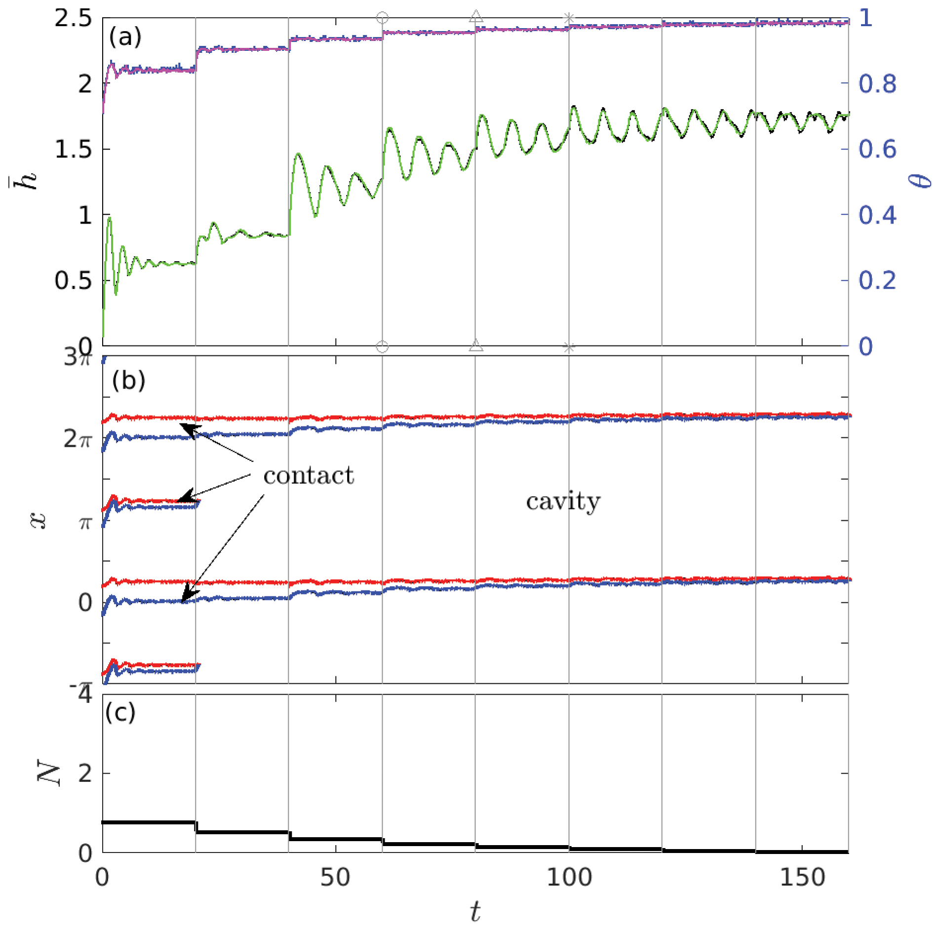
Figure 6 Using the same plotting scheme as in Fig. 3, dynamic cavity evolution under step changes in N with a fully permeable bed, $P=(\mathrm{0},a)$, using a smaller initial value of N than in Fig. 5. In each panel the solution for the same mesh as used in Fig. 5 and all remaining figures is shown in black and blue in panel (a) and blue and red in panel (b). The solution for a mesh with twice the resolution at the bed is shown in magenta and green in panel (a) and black in panel (b).

3.3 Dynamic cavity connection

The rather long time interval over which the solution in Fig. 3 is plotted makes it impossible to see the fine detail of ice–bed gap evolution when a cavity expands rapidly across the top of a bed protrusion, as happens shortly after t=78. Such rapid expansion corresponds to an isolated part of the bed becoming connected to the subglacial drainage system and is therefore of particular interest.

In Fig. 7, I focus on that rapid expansion (moving the time origin to the instant that N undergoes the step change that leads to cavity expansion). Prior to expansion, the cavity is in a quasi-steady state (see Sect. 3.1 and Fig. 2a) at N=1.05. In addition to replotting the solution in Fig. 3, corresponding to a step down to N=0.70, I also compute the response to larger step changes in order to determine how step size affects the speed and nature of the cavity expansion.

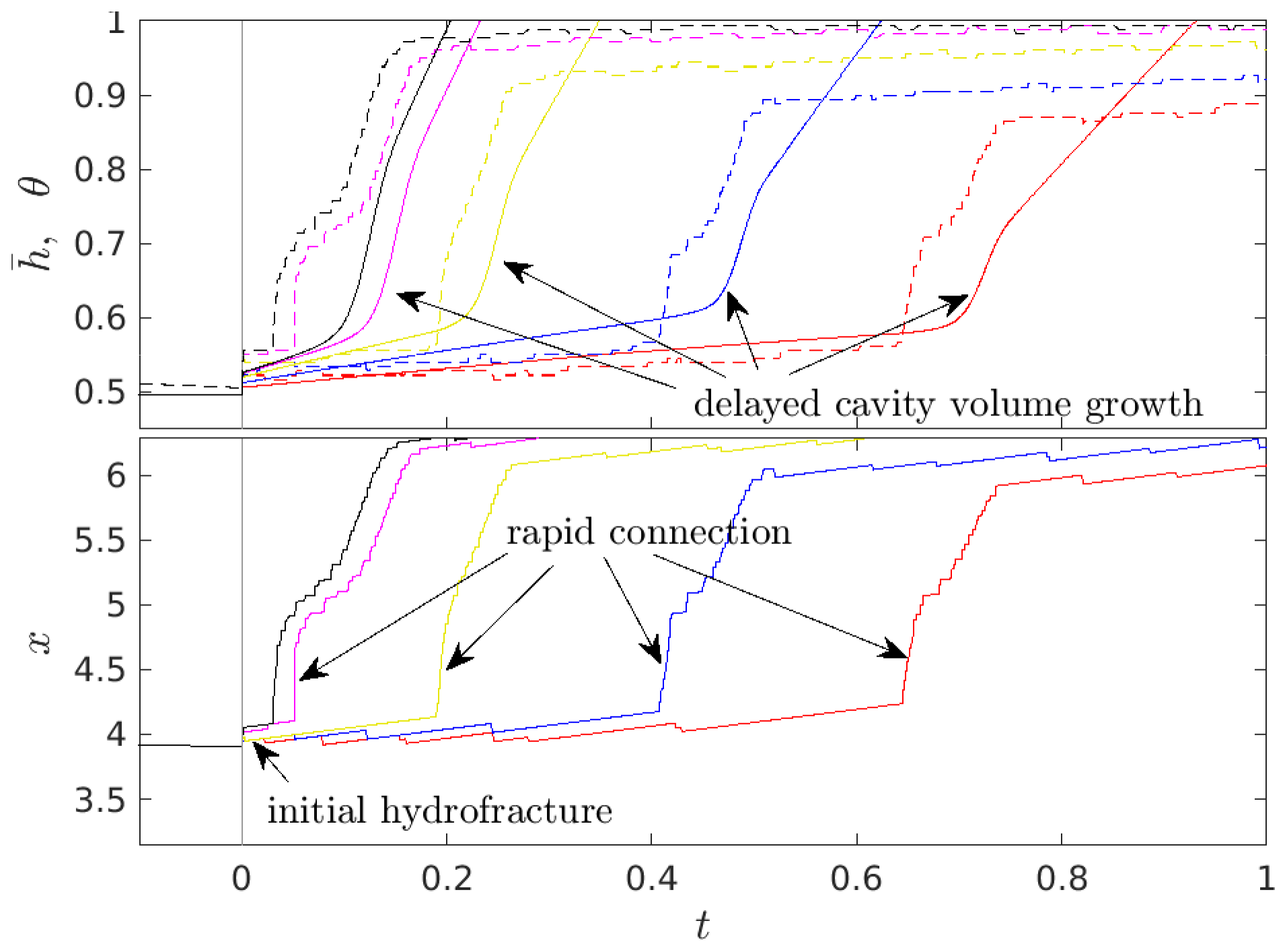
Figure 7 Cavity connection under different step changes in N. The cavity is initially in a (quasi-)steady state with N=1.05 and a single small cavity attached to the larger bed protrusion in the bed. N is then changed abruptly at t=0 to values of 0.70 (red), 0.47 (blue), 0.21 (yellow), 0.041 (magenta), and $\mathrm{1.6}\times {\mathrm{10}}^{-\mathrm{3}}$ (black). (a) Cavitation ratio θ (dashed) and mean cavity depth $\overline{h}$ (solid) against time t. (b) Downstream cavity end-point position against time t.

Immediately after the drop in N, $\overline{h}$ and θ undergo a rapid but small increase. The increase in cavity size is larger when N drops to a lower value and is the result of elastic uplift of the ice around the edge of the pre-existing cavity. The speed of the initial expansion is much faster than the advective speed $\overline{u}$ and is presumably controlled by the gap permeability κ as is the case in hydrofracture problems with negligible fracture toughness (Mitchell et al., 2006). I have, however, not checked for the effect of κ numerically.

Importantly, this initial “hydrofracture” (which is not a hydrofracture in the true sense, as it corresponds to a pre-existing fracture being re-opened) has a very limited extent. In fact, the same initial fracture occurs every time that N goes through a step change, regardless of whether the cavity expands significantly afterwards. For step changes in N that do not lead to large-scale expansion by drowning of a smaller lee-side protrusion, that brief hydrofracture episode is the only part in the process of cavity enlargement that involves elastic effects (in the sense of occurring over a shorter interval than the Maxwell time). This initial hydrofracture-like rapid increase in cavity size is followed by a period of much more moderate cavity growth, with gradual growth in $\overline{h}$ and the downstream cavity end point advancing at speeds comparable to $\overline{u}$ or slower. The rate of cavity growth is again greater for lower N.

In interpreting the results for θ and cavity end-point position in Fig. 7, recall that the numerical method uses a travelling frame that moves precisely at speed $\overline{u}$, and cavity end points are by construction located at the finite-volume cell centres in that travelling frame. This once more explains the non-smooth appearance of the plots in Fig. 7b and why cavity end points can appear to move backwards, especially for larger values of N (the blue and red curves). That backward motion corresponds to one of the advected finite-volume cells going from ice–bed separation to contact. Where such backward motion of the cavity end point does not occur, the cell centre that is the cavity end point moves precisely at $\overline{u}$. Consequently, the relatively coarse spatial resolution limits the ability to resolve variations in the speed of the cavity end point.

The second phase of slower cavity growth is the result of viscous deformation. Only once the downstream cavity end point has advanced significantly downstream does the rapid expansion (or connection) of the cavity past the smaller bed protrusion occur, marked as “rapid connection” in Fig. 7b. The precise location of the downstream cavity end point at which this occurs depends slightly on the value of N, with a less-advanced cavity end point at the onset of cavity connection if N is lower (c=4.08 at $N=\mathrm{1.6}\times {\mathrm{10}}^{-\mathrm{3}}$ versus c=4.23 at N=0.70). The cavitation ratio is relatively uniform at θ≈0.56 for all forcing effective pressures at the onset of connection.

The subsequent rapid expansion of the cavity (following the second phase of slower cavity growth and corresponding to the “drowning” of the smaller bed protrusion) can be separated into two parts: an initial advance of the cavity end point from c≈4.1 to c≈4.5 over a time interval around 10⁻², somewhat shorter than a single Maxwell time. This part of the cavity expansion is marked with rapid connection in Fig. 7b and is effectively another example of hydrofracture. It is not accompanied by any noticeable change in $\overline{h}$. Subsequently, cavity expansion continues more slowly to a final position around x≈6, though the cavity end point continues to migrate at speeds greater than $\overline{u}$ during this phase. It is only during this slower expansion that the cavity depth $\overline{h}$ increases more rapidly: this phase is much longer than a single Maxwell time and is again associated with viscous deformation of the ice. That increase in depth continues after the cavity end point stops advancing rapidly and eventually leads to overshoot of the equilibrium depth and the oscillations in Fig. 3a.

Figure 8 illustrates the evolution of cavity shape for the case of a drop in N to 0.47. The initial condition is shown in panel (a) and the aftermath of the initial hydrofracture in panel (b). The difference between the two is all but imperceptible. Cavity shape immediately before the rapid expansion is shown in panel (c), with the cavity end point having migrated a short but noticeable distance to the top of the smaller bed protrusion. The subsequent rapid expansion of the cavity leads to an extended, thin ice–bed gap extending downstream of the pre-existing cavity (panel d): this corresponds to the rapid increase in θ accompanied by an insignificant change in $\overline{h}$.

The gap then thickens more slowly (panel e), leading to oscillatory behaviour (panels f–j; these later times are not shown in Fig. 7). The final steady state is shown in panel (k). Note that panels (f)–(j) illustrate the mechanism for overshoot oscillations described in Sect. 3.2: the contact area on the more prominent upstream bump migrates downstream and shrinks between panels (f) and (h), causing a reduced vertical velocity and subsequently a reduced cavity height being advected downstream as shown in panel (i). In fact, contact area undergoes much more significant change in size and location here than it does in later oscillations: in panel (g), there are two contact areas, one on the larger bed protrusion upstream and one on the smaller one downstream, while in panel (h), there is a water-filled gap with thickness above the threshold for contact identification everywhere. The main contact area on the larger bed protrusion subsequently migrates upstream again as a result of the reduction in cavity height, with a steeper average contact angle in panel (i) than (g), leading to larger vertical velocities. These in turn cause increased uplift once more and therefore the subsequent increase in cavity height in panel (j).

I illustrate the oscillation mechanism further in Fig. 9, where I plot the mean contact angle of all contact areas against time in the same plot as mean cavity roof height $\overline{h}$ and cavitation ratio θ. The oscillation mechanism is most clearly seen later in the interval shown: here, the contact angle is shown as red peaks when $\overline{H}$ is increasing most rapidly and then steadily decreases around the maximum of $\overline{h}$, as advection causes the downstream end of the cavity to enlarge and the re-contact point to migrate downstream. In time, downstream migration and reduction in contact angle cause $\overline{h}$ to decrease again.

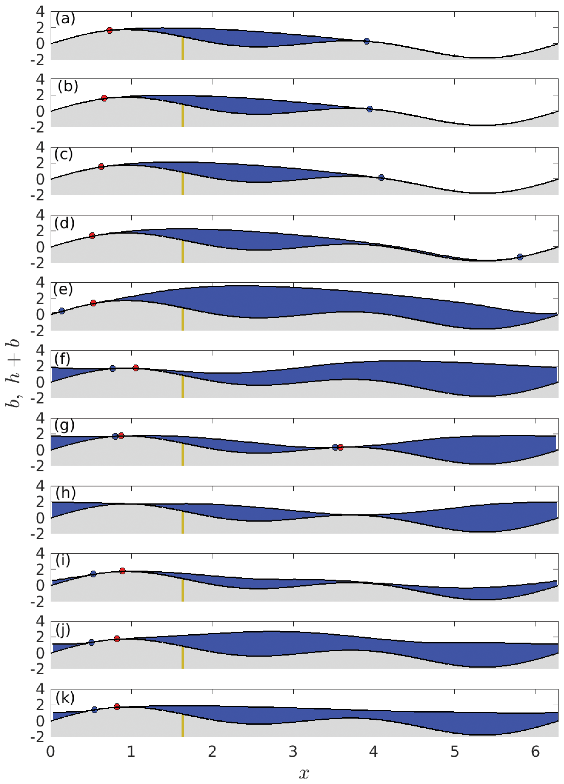
Figure 8 Cavity shapes for a step change from N=1.02 to N=0.47 (the blue curves in Fig. 7) at (a) t=0, (b) $t={\mathrm{10}}^{-\mathrm{3}}$, (c) t=0.32, (d) t=0.49, (e) t=1.35, (f) t=3.39, (g) t=4.62, (h) t=5.16, (i) t=6.61, (j) t=8.70, and (k) t=120. Red dots correspond to upstream cavity end points and blue dots to downstream end points.

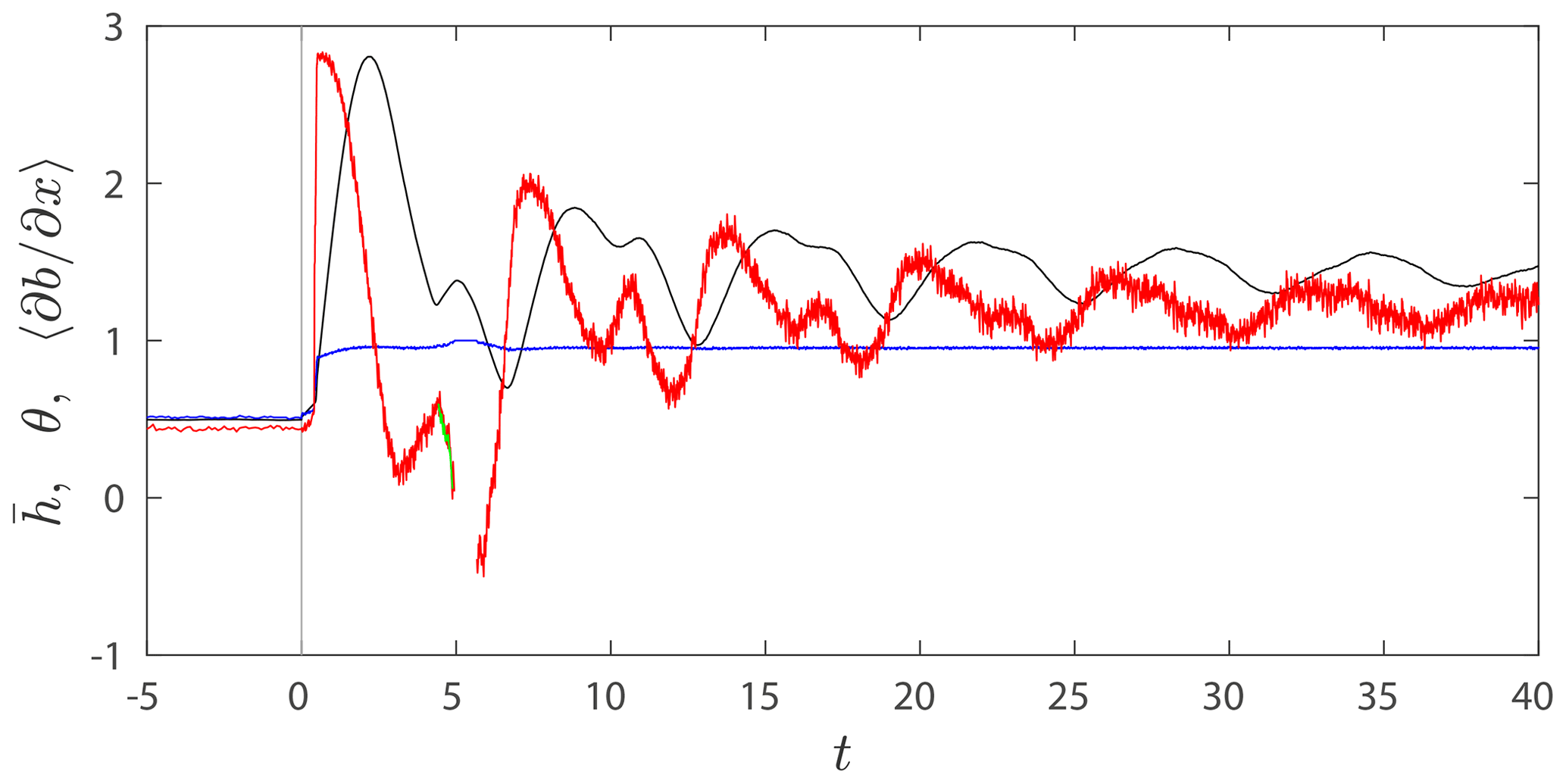
Figure 9 Cavity height $\overline{h}$ (black), cavitation ratio θ (blue), and mean contact angle $〈\partial b/\partial x〉$ (red and green) corresponding to a step change from N=1.02 to N=0.47 at t=0 (for $\overline{h}$ and θ, these are the blue curves in Fig. 7, plotted for a longer time interval). For each contact area $(c_j,b_{j+\mathrm{1}}$, I compute the mean contact angle as $〈\partial b/\partial x〉=(b_{j+\mathrm{1}}-c_j{)}^{-\mathrm{1}}{\int }_{c_j}^{b_{j+\mathrm{1}}}\partial b/\partial x\mathrm{d}x=(b\left(b_{j+\mathrm{1}}\right)-b\left(c_j\right))/(b_{j+\mathrm{1}}-c_j)$. Note that there is an interval from t=4.94 to t=5.69 during which the code detects no contact area (a sufficiently deep water layer is present everywhere), and there are two contact areas between t=4.43 and t=4.88.

3.4 Overpressured cavities

In the computations above, I have focused on a permeable bed section P immediately in the lee of the largest bed protrusion. As explored in Part 1, the location of the permeable bed section has major qualitative implications for steady-state results. These are replicated in the dynamic model. Figure 10 shows results analogous to Fig. 3, but with P centred on the downstream side of the smaller bed protrusion at x_P=4.64.

Two solutions are plotted, both of them identical up to t=260. One is forced by N being reduced to close to zero and then increasing again. The other is indicated as “overpressure solution” by arrows and has N lowered successively to −0.46 and −0.96. In line with the results in Part 1, we see relaxation to steady states for all positive N, as well as at $N=-\mathrm{0.46}$, which lies above the critical value $N_{\mathrm{drown}}=-\mathrm{0.79}$ in Fig. 5 of Part 1. In fact, with a substantial uncavitated portion of the bed, relaxation to steady state is relatively rapid with limited overshoot of cavity size $\overline{h}$ as is also the case for t<78 in Fig. 3. Only for the lowest value of $N=-\mathrm{0.96}$ used does complete detachment of ice from the bed occur, with θ reaching unity (Fig. 10a).

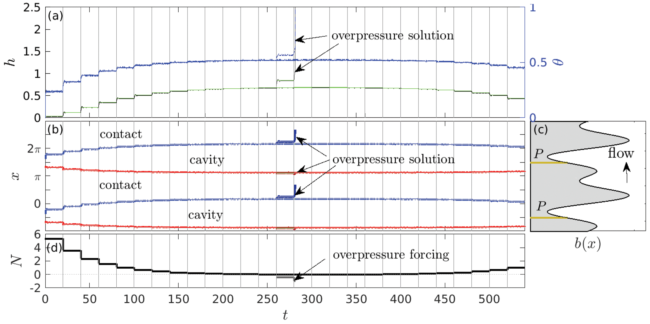
Figure 10 Using the same plotting scheme as in Fig. 3, dynamic cavity evolution under step changes in N with a permeable bed on the downstream side of the smaller bed protrusion, with P={4.64}. The solution indicated by arrows corresponds to negative forcing effective pressure N and departs at t=260 from the solution not indicated by arrows.

3.5 Pressure in isolated cavities

In Part 1, I showed that steady-state effective pressure in isolated cavities is remarkably insensitive to changes in the effective pressure N in the ambient drainage system. This is far from true of the dynamic response of an isolated cavity to changes in N. The dynamic response is of significant interest, as this is what a subglacial water pressure sensor would measure if connected to such an isolated cavity.

Here, I give three examples in which the connected cavity in the lee of the larger bed protrusion (with x_P=1.64) is forced periodically as shown in panels (b1)–(b3) of Fig. 11. The period and amplitude of the forcing pressure oscillation differ between the columns of Fig. 11, with a period of π (column 1), 2π (column 2), and 4π (column 3). For reference, note that the advective period is $a/\overline{u}=\mathrm{2}\mathit{\pi }$. The green curves in panels (b1)–(b3) show that effective pressure N_M “measured” at the location marked M in panel (c). Note that the fixed location of M corresponds to a sensor installed at the glacier bed itself, which is unusual (Lefeuvre et al., 2015): in most field installations, pressure sensors are placed in boreholes and advected with the ice, corresponding to a location moving at velocity $\overline{u}$ in our model. Vertical grey lines in rows with labels (a) and (b) correspond to times at which ice–bed contact is made or lost on the smaller bed protrusion upstream of M, while panels (a1)–(a3) show cavity end points as in Fig. 3b.

In column 1, a relatively small isolated cavity forms before periodic behaviour is established. That cavity then remains isolated throughout the pressure cycle. The effective pressure N_M in that isolated cavity is in antiphase with the forcing effective pressure N in the connected cavity. This behaviour is familiar from field observations in parts of the glacier bed that are not hydraulically connected (Andrews et al., 2014; Rada and Schoof, 2018). A simple way to interpret the antiphase pressure variations is in terms of the portion of overburden supported by the isolated cavity (Murray and Clarke, 1995; Lefeuvre et al., 2015): when forcing effective pressure N is low, a larger fraction of overburden is supported by the connected cavity, reducing normal stress on the isolated cavity and therefore also reducing water pressure in the cavity, which corresponds to a higher effective pressure N_M (defined as overburden minus water pressure in the isolated cavity).

When the forcing oscillations have a somewhat lower frequency (column 2), there are more significant changes in the ice–bed contact area on the smaller bed protrusion. An isolated cavity now forms during every other period of the forcing pressure oscillation (that is, the solution is periodic with a periodicity twice that of the forcing). In each case, the cavity roof makes contact with that protrusion after a maximum in N (panel a). For most of the intervals in which there is no contact on top of the smaller protrusion (see panel a2), the two effective pressures are nearly equal: N_M≈N to a very close approximation. There is, however, an extended interval prior to contact being re-established, during which forcing effective pressure N is high and the measured effective pressure N_M drops below N. Even though the two cavities are connected across the top of the bed protrusion, there is a sufficiently narrow constriction in the ice–bed gap to support a significant pressure gradient. As the animation of cavity shape evolution corresponding to Fig. 11 in video V2 in the Supplement shows, that constriction is advected downstream and eventually re-contacts with the bed. Once that happens, the measured effective pressure rapidly increases and then goes through an antiphase pressure oscillation while the cavity around the point M is isolated. When the connection between the cavities is re-established once more, the effective pressure at M rapidly equilibrates with that at P.

The forcing pressure oscillation in column 3 is even slower and of larger amplitude than those in columns 1 and 2. Here, the solution has the same periodicity as the forcing, with a contact area forming on the smaller bed protrusion upstream of M when forcing effective pressure N is large. A reduced ice–bed gap size and consequent contact at the top of bed protrusions might be expected at large N, but contrast with the solution in column 2 for a higher forcing frequency. As in column 2, N_M≈N when the cavities are connected, with a brief interval around t=15 during which N_M is significantly lower than N after connection is re-established. Again, this results from a narrow ice–bed gap across the top of the smaller bed protrusion.

When the cavities become fully disconnected, N_M does not simply go through part of an antiphase pressure oscillation, unlike in column 2. After disconnection, N_M initially drops while N increases, with N_M reaching negative values. Subsequently, however, N_M rises again and relaxes to a near-zero value while the forcing effective pressure N is still increasing. It is tempting to ascribe the difference in behaviour between columns 2 and 3 to the slower period of forcing oscillation in column 3; given the long timescale for relaxation to steady state evident in Fig. 3, it is unclear to what extent that interpretation is appropriate.

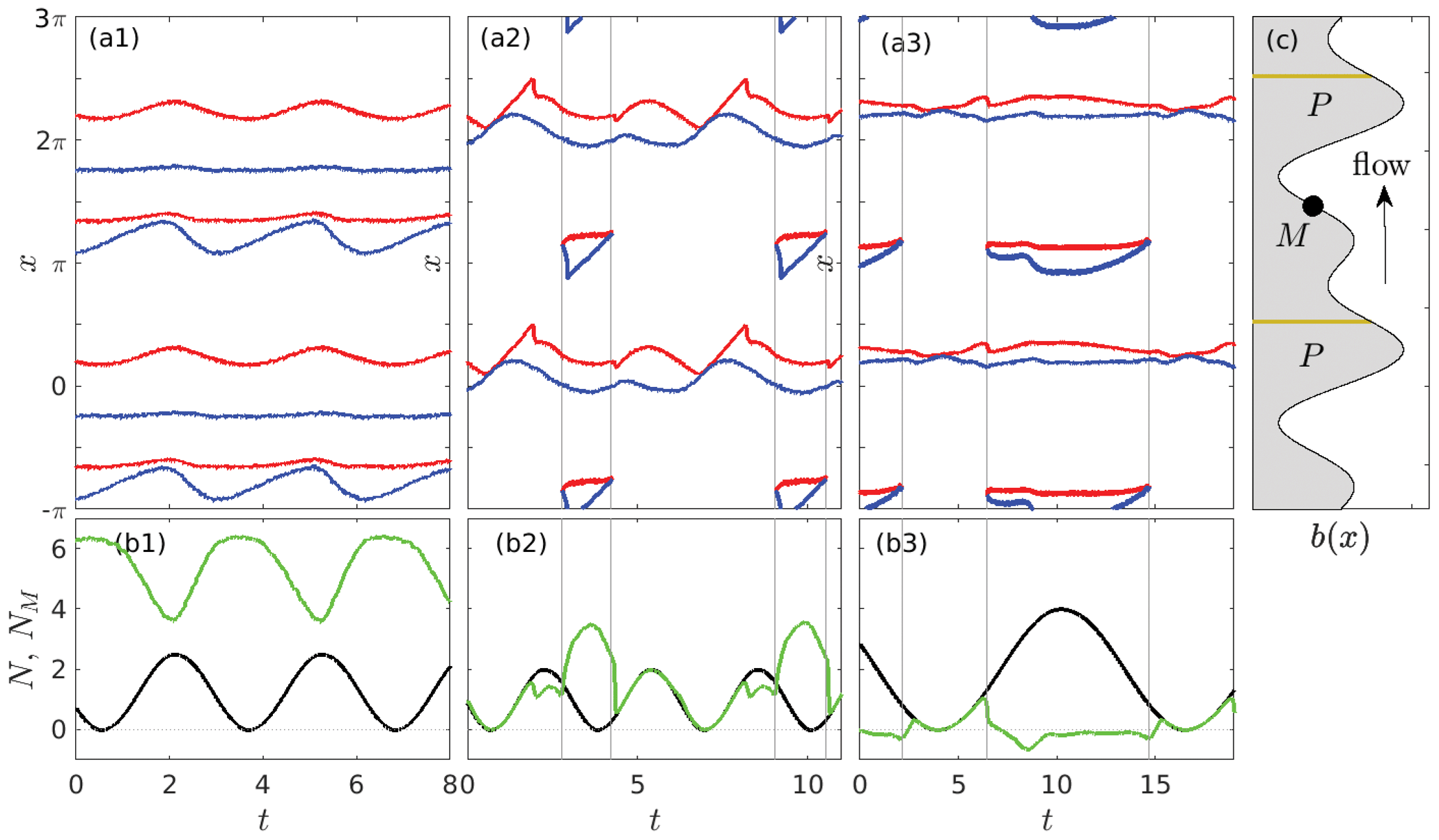
Figure 11 Using the same plotting scheme as in Fig. 3, dynamic cavity evolution under oscillatory forcing. (a) Time series of upstream (red) and downstream (blue) cavity end points. Vertical lines indicate when contact is made and lost with the smaller bed protrusion. (b) Corresponding bed geometry, with the permeable portion P indicated in beige. The circular black marker M indicates location where the effective pressure N_M is measured. (c) Time series of effective pressure N (black) and locally measured effective pressure (in green, given by the dimensionless variable −p_w in the model) at the location of the black marker in panel (b).

4 Discussion

4.1 Subglacial hydrology

In Part 1, I showed that for a steady-state model, connections between cavities are created and destroyed at critical values of N and that the critical value for connection to a previously uncavitated part of the bed is lower than the critical value at which that connection is closed or at which a connection to a previously isolated cavity is established. The results in the present paper are consistent with these observations: Fig. 2 demonstrates that at N=1.053, hydraulic isolation of the downstream side of the smaller bed bump can be maintained in steady state (panel a). However, a single larger cavity can equally extend across the top of the smaller bed bump at the same effective pressure (panel b), and the lee side of the smaller bed bump only becomes hydraulically isolated at higher effective pressures as in panel (c). A careful inspection of the final steady states in Figs. 3 and 4 also confirms that connection to a previously uncavitated part of the bed happens at lower effective pressure (shortly after t=78 in Fig. 4 at N=0.70) than either subsequent isolation of part of the newly extended cavity (shortly after t=638 in the same figure at N=1.58) or reconnection (shortly after t=40 in Fig. 4 at N=1.05).

One might therefore be tempted to parameterize cavity connection in large-scale drainage models in terms of effective pressure N reaching a threshold value. The insights from steady-state calculations are, however, misleading in a dynamic situation: Fig. 7 shows that it is not the instantaneous drop in N below some critical value that causes a hydraulic connection to be established. Instead, a drop in N causes mean cavity depth $\overline{h}$ and cavitation ratio θ (the fraction of the bed that is cavitated) to grow. That growth eventually allows hydraulic connection as a bed protrusion on the downstream side is “drowned”. In fact, θ reaching a critical value appears to be the best predictor for connection, though mean cavity depth $\overline{h}$ at connection varies by a relatively small amount, and it is plausible that a critical value h_c could be defined.

This result is at least consistent with the previous modelling approach of Rada and Schoof (2018). Beyond that, matters become significantly more complicated: Fig. 7 pertains to a hydraulic connection being made by a cavity rapidly extending past the top of a smaller bed bump into a portion of the bed that was previously at low pressure but uncavitated. If that region subsequently becomes isolated again due to the cavity roof being lowered at increased N, the mean cavity depth $\overline{h}$ will remain larger than at the time the original connection was made, precisely because there is now a second cavity on the downstream side of the smaller bed bump (see Fig. 3a). In any case, it is not possible to use the same critical value h_c to determine whether there is a connection or not.

A plausible alternative to having a simple critical value h_c for cavity connection in a large-scale model is to recognize that θ has also increased, and the definition of a critical value for connection should involve not only $\overline{h}$ but also θ. Doing so must then also reflect the observation in Part 1, namely that connection to a previously uncavitated part of the bed happens at a lower critical effective pressure N than reconnection to a pre-existing isolated cavity: however, the steady states of $\overline{h}$ and θ depend on N, and the critical combination of $\overline{h}$ and θ that defines connection must be such that reconnection happens more easily than connection to an uncavitated part of the bed.

These observations point to a need to extend drainage models to describe the evolution of not only $\overline{h}$, but also of at least one more independent state variable like θ. Note that $\overline{h}$ and θ are not simply proxies for each other (Gilbert et al., 2022): during the cavity connection events in Fig. 7, θ increases much faster than $\overline{h}$ initially, as a narrow ice–bed gap is formed (see also Fig. 8d), and θ is clearly the more important measure of connectedness here.

Any attempt to amend subglacial hydrology models along these lines, however, faces another conundrum: as currently formulated, existing subglacial drainage models use an evolution equation for $\overline{h}$ of the generic first-order form (2), which is essentially a local ordinary differential equation (there being no spatial derivatives). The equation being first-order in time, $\overline{h}$ should then monotonically relax to a stable steady-state solution under conditions of constant sliding velocity u_b and effective pressure N.

Figures 3, 4, 5, and 10, however, all show $\overline{h}$ overshooting its steady-state solution with an oscillatory approach to equilibrium. This is incompatible with Eq. (2): any dimensionally reduced representation of cavity evolution (relative to the full dynamic model developed in this paper) must involve more than one state variable. In a similar vein, the solution with time-dependent forcing in Fig. 11b shows a period doubling of the solution relative to the forcing. This is not necessarily incompatible with a model of the form (2), but in typical implementations such as Werder et al. (2013), Eq. (2) is linear in $\overline{h}$, which does preclude period doubling.

It is conceivable that a model of the form (2) could still be appropriate in many situations: the marked oscillations in Figs. 3, 4, and 5 are all associated with a single contact area per bed wavelength in a periodic bed, and it is unclear whether similar behaviour would result on an aperiodic bed (or a bed with a very long period, in which case multiple contact areas would remain even at low N; see Schoof, 2002, Chap. 2). Similarly, the solution in Fig. 11b involves contact areas shrinking to very small sizes during the pressure cycles. The fact that the oscillations are minor when there is significant ice–bed contact or multiple contact areas and that the overshoot in $\overline{h}$ past its steady-state value is generally small then suggests that the simple model (2) could capture cavity evolution well in the more realistic setting of an aperiodic bed. Further research using a more sophisticated approach to solving the model equations on larger domains with irregular beds would be needed to address this question.

If, on the other had, the overshoot oscillations are an important part of the evolution of the drainage system, then the set of variables that an extended model needs to consider is most likely larger than simply $(\overline{h},\mathit{\theta })$. As observed in Figs. 3 and 4, the oscillations in $\overline{h}$ seem to involve the contact area moving back and forth across the top of the most prominent bed bump while remaining of approximately constant size. That is, θ remains nearly constant during the oscillations. The addition of a dynamic variable θ while making v_o or v_c depend on θ is therefore unlikely to reproduce oscillatory behaviour, since θ should be nearly constant during the oscillations: a proxy for contact position rather than size appears to be necessary.

The ad hoc addition of dynamical variables is clearly a disturbing prospect in the absence of a clear roadmap for how closure should be achieved. Once a set of such dynamical variables is identified, then perhaps the obvious next step would be to try to arrive at a closed set of equations for the evolution of these dynamical variables not by means of qualitative physical insight and subsequent parameter fitting, but by treating their evolution as being governed by a dynamical system that can be represented by a neural network, which in turn can be trained on output from a detailed process-scale model such as that described here (e.g. Brenowitz and Bretherton, 2018, 2019). That procedure, however, still involves an expert choice of dynamical variables to use in the large-scale model, and one would hope for something better: a method of optimally choosing these dynamical variables.

4.2 Interpretation of field measurements

The discussion above has focused on the implications of the local-scale model results in the present paper for large-scale subglacial models. The same results also have implications for the interpretation of field observations: a perhaps obvious consequence of hydraulic isolation of the bed is that the usual basal water pressure may no longer be smoothly varying in space and in fact has no physical meaning in areas of ice–bed contact. For a highly permeable bed, a pressure sensor in a borehole that terminates on an ice–bed contact still measures the water pressure in any surrounding cavities, since water from those cavities can readily access the borehole through the bed. This is no longer true for an impermeable bed. Measuring borehole water pressure where a borehole terminates on an ice–bed contact area then records the peculiarities of pressure evolution in the isolated borehole, which itself is of unknown shape and must preserve its volume (assuming the borehole has closed, as is typically the case; see e.g. Rada and Schoof, 2018) while subject to a non-uniform stress field at the bed. The measurement in that situation no longer reflects conditions at the bed in a simple way.

By contrast, when a sensor is connected to an isolated cavity, the pressure measurement records the water pressure in the cavity. The latter again needs to preserve its own volume as modelled in the present paper. The pressure response of isolated cavities to temporally varying forcing pressures is sensitive to the timescales involved. For high-frequency oscillations in forcing (faster than the deformation timescale $a/\overline{u}$), the pressure response in isolated cavities is in antiphase with the forcing (Fig. 11a1), reflecting variations in the fraction of overburden supported by connected and isolated cavities. When forcing effective pressure N is low, a larger fraction of overburden is supported by the connected cavity, reducing normal stress on the isolated cavity and therefore also reducing water pressure in the cavity, which corresponds to a higher effective pressure N_M (defined as overburden minus water pressure in the isolated cavity). Antiphase pressure oscillations of this type are familiar from observational records (Murray and Clarke, 1995; Lefeuvre et al., 2015; Rada and Schoof, 2018) and, as shown by my results, do not require variations in ice velocity caused by the forcing effective pressure, since I have set sliding velocity to a constant (see also Lefeuvre et al., 2018).

For slower forcing oscillations, temporary connections between cavities can be established, corresponding to “switching events” observed in borehole pressure records (Murray and Clarke, 1995; Hubbard et al., 1995; Rada and Schoof, 2018). During intervals of disconnection, the pressure response of the isolated cavity may again be in antiphase with forcing (Fig. 11a2), which is somewhat similar to the “alternating borehole” record in Fig. 5 of Murray and Clarke (1995) and Fig. 7 of Rada and Schoof (2018). This ceases to be the case during pressure oscillations that are significantly longer than the deformation timescale $a/\overline{u}$ (Fig. 11a3): in that case, the effective pressure during hydraulic disconnection does not satisfy any simple relationship with the forcing effective pressure, making interpretation of the recorded “data” challenging. Hydraulic connections between cavities can also be poor but not fully closed for extended intervals as a result of small ice–bed gaps: these intervals most likely would not be interpreted as representing a hydraulic connection in observational data, and it is difficult to determine from the observed pressure time series when complete disconnection occurs.

4.3 Model improvements

There are likely to be many areas in which the model described here can be improved, ranging from a careful analysis of the numerical method used to practical implementation issues such as the use of a potentially more suitable finite-element basis, adaptive time stepping, and adaptive meshing as well effective parallelization. In addition, there are physical processes that the present work has been unable to consider.

The most obvious among the latter is the effective solution of the model in three dimensions to capture changes in hydraulic connectivity: in a two-dimensional model, it is impossible to establish connectivity from one end of the domain to the other unless ice–bed contact is lost everywhere, which is not a physically reasonable situation. It is only in three dimensions that full end-to-end connectivity (meaning water is free to flow from one side of the domain to the other) can coexist with continuing ice–bed contact. Similarly, I have focused purely on the hydrological aspects of dynamic cavity evolution and do not attempt to address the question of a friction law for dynamically evolving subglacial cavities, which would be a worthwhile addition in its own right (de Diego et al., 2022; Gilbert et al., 2022), as would a consideration of non-constant viscosity in the ice. Lastly, the ability to capture flowing water through linked cavities in three dimensions would make the model a tempting test bed for studying spontaneous channelization at the process scale by adding a term representing roof melting to the kinematic boundary conditions (9) or (16f) (see also Kamb, 1987, and Dallaston and Hewitt, 2014). To avoid spuriously localized feedbacks between water depth and dissipation-driven melting, it may then be necessary to dispense with the simple local formula for water flux in terms of water depth as in Eq. (11c) by considering a horizontal turbulent viscosity (see also Creyts and Schoof, 2009).

5 Conclusions

In this paper, I have formulated a viscoelastic model for ice sliding over a rigid and mostly impermeable bed, allowing for the formation of cavities in which water is dynamically redistributed by an active local drainage system. The model is capable of describing the dynamic extension of subglacial cavities as bed obstacles progressively become submerged by water sourced from a localized water supply connected to an ambient drainage system at prescribed effective pressure. In the same vein, the model is capable of capturing the formation and evolution of isolated subglacial cavities that trap a fixed water volume after becoming isolated. Its steady-state results agree well with the results of a simpler, two-dimensional, and purely viscous steady-state model that is solved by an entirely different numerical method.

The model lends some credence to existing approaches to modelling hydraulic isolation of the glacier bed in large-scale models using a threshold in mean cavity size to define connectivity, but it also suggests that significant modifications to those models may be required. For instance, it suggests that the cavitation ratio measuring the horizontal extent of ice–bed separation needs to be considered separately from the mean ice–bed gap thickness, especially when modelling the rapid expansion of cavities as previously uncavitated low-pressure regions of the bed are flooded by water: the cavitation ratio evolves faster and is a better predictor of subglacial connectivity than ice–bed gap thickness, and the two variables are not simple proxies for one another (see also Gilbert et al., 2022). Adding the relevant physics to a large-scale subglacial drainage model, however, requires the addition of model variables whose evolution is not described by an existing simple parameterization, and future research needs to be directed towards constructing such parameterizations based on process model output.