the Creative Commons Attribution 4.0 License.
the Creative Commons Attribution 4.0 License.
 | 10 Nov 2023
Investigating the spatial representativeness of East Antarctic ice cores: a comparison of ice core and radar-derived surface mass balance over coastal ice rises and Dome Fuji
Marie G. P. Cavitte
Hugues Goosse
Kenichi Matsuoka
Sarah Wauthy
Vikram Goel
Rahul Dey
Bhanu Pratap
Brice Van Liefferinge
Thamban Meloth
Jean-Louis Tison
Surface mass balance (SMB) of the Antarctic Ice Sheet must be better understood to document the current Antarctic contribution to sea-level rise. In situ point data using snow stakes and ice cores are often used to evaluate the state of the ice sheet's mass balance, as well as to assess SMB derived from regional climate models, which are then used to produce future climate projections. However, spatial representativeness of individual point data remains largely unknown, particularly in the coastal regions of Antarctica with highly variable terrain. Here, we compare ice core data collected at the summit of eight ice rises along the coast of Dronning Maud Land, as well as at the Dome Fuji site, and shallow ice-penetrating radar data over these regions. Shallow radar data have the advantage of being spatially extensive, with a temporal resolution that varies between a yearly and multi-year resolution, from which we can derive a SMB record over the entire radar survey. This comparison therefore allows us to evaluate the spatial variability of SMB and the spatial representativeness of ice-core-derived SMB. We found that ice core mean SMB is very local, and the difference with radar-derived SMB increases in a logarithmic fashion as the surface covered by the radar data increases, with a plateau ∼ 1–2 km away from the ice crest for most ice rises, where there are strong wind–topography interactions, and ∼ 10 km where the ice shelves begin. The relative uncertainty in measuring SMB also increases rapidly as we move away from the ice core sites. Five of our ice rise sites show a strong spatial representativeness in terms of temporal variability, while the other three sites show that it is limited to a surface area between 20–120 km2. The Dome Fuji site, on the other hand, shows a small difference between pointwise and area mean SMB, as well as a strong spatial representativeness in terms of temporal variability. We found no simple parameterization that could represent the spatial variability observed at all the sites. However, these data clearly indicate that local spatial SMB variability must be considered when assessing mass balance, as well as comparing modeled SMB values to point field data, and therefore must be included in the estimate of the uncertainty of the observations.
- Article
(3634 KB) - Full-text XML
-
Supplement
(8194 KB) - BibTeX
- EndNote


Quantifying current mass balance and predicting its future evolution are key to constraining the present and future rate and timing of sea-level rise due to Antarctic freshwater input. Mass balance is the result of the net equilibrium between surface mass balance (the net accumulation of snow) at the surface of the ice sheet and the dynamic losses at the grounding line (Lenaerts et al., 2019). The thermodynamics of the atmosphere indicate that, with rising temperatures, there will be rising saturation specific humidity (Clausius, 1850). We should therefore expect increasing snow accumulation over the Antarctic Ice Sheet, which could potentially offset grounding line dynamic losses, for a while at least. Over the past decades, temperatures have been steadily rising, with a large spatial variability over the globe (Arias et al., 2021). To see if snow accumulation is increasing as a result over Antarctica, we can look at direct measurements of accumulation such as firn cores, ice cores and stake measurements, each with their own measurement uncertainties. Firn and ice cores (which we refer to as ice cores from here on out) provide the highest-temporal-resolution records. The Antarctic coastal region is getting most of the accumulation due to a combination of source proximity, low elevation and topographic precipitation forcing (e.g., Lenaerts et al., 2019). However, when examining the ice core records from this region, they all have very different trends (Medley and Thomas, 2019). A lot of temporal variability is likely introduced by atmospheric rivers (Maclennan et al., 2022), with a high impact along the coastal areas of East Antarctica. Ice cores provide a record of surface mass balance (SMB) at the seasonal to annual temporal resolution in the shallowest part of the ice column (Fudge et al., 2016; Philippe et al., 2016; Hoffmann et al., 2022). Resolution decreases with depth as snow compacts, and lateral ice flow augments the layer thinning. Ice cores or point measurements can give a high temporal resolution for SMB, but their spatial sampling is limited, and their surface footprint is quite small. Moreover, wind-driven processes active at the surface can redistribute deposited snow (Frezzotti et al., 2004, 2007; Lenaerts et al., 2019; Kausch et al., 2020; Wever et al., 2022). Measuring SMB in one point (i.e., ice cores) could therefore sample an accumulation record that displays locally higher or lower SMB rates than over the wider region because of the selected location. Wever et al. (2022) have shown that high wind speeds can re-mobilize snow and produce depositional patterns that are spatially variable on the scale of a few meters. Kausch et al. (2020) have also shown how the interaction of coastal domes' orography and surface winds can create meter- to kilometer-scale SMB spatial heterogeneity. Furthermore, averaging many records in close proximity does not significantly improve the signal-to-noise ratio in the ice core records (Cavitte et al., 2020; Münch et al., 2021). To predict future mass balance changes, we rely on model simulations. Model simulations are validated using instrument data and paleo data, as well as ice core data for SMB model outputs. However, observations and simulations do not always agree (Agosta et al., 2019; Goel et al., 2022; Pratap et al., 2022). The models with the highest spatial resolution to be compared to point measurements are regional climate models (RCMs). RCMs also have specific adaptations of their physics for the polar regions (van Wessem et al., 2018; Fettweis et al., 2013). Although RCMs have smaller grid cells than global climate models, grid cells remain at best 5.5×5.5 km in size (van Wessem et al., 2018). The discrepancies between model results and ice core measurements might be partly due to the difference in their spatial representativeness.
Radar data can be used to investigate ice cores' spatial representativeness. By connecting radar internal reflecting horizons (IRHs) to ice core sites, SMB rates can be derived over the entirety of a traced radar survey. The absolute ages are determined from the ice core age–depth timescale (Verfaillie et al., 2012; Cavitte et al., 2016; Le Meur et al., 2018). Radar-derived absolute SMBs are therefore not independent of the ice core SMB, but spatial variations in the SMB can be measured between the ice core site and the wider surveyed area. Ground-based radar surveys are often relatively dense over areas of a few tens of square kilometers, so they provide SMB constraints at a spatial scale comparable to the models. This raises the new opportunity that, instead of comparing ice core point observations to model simulations, we could compare the radar-derived SMB signal averaged spatially over a model's grid size.
In this study, we compile various radar-derived SMB data sets and describe their spatial variability referenced to co-located ice core SMB. We compare ice core pointwise measurements to wider spatial averages obtained from subsets of the radar surveys to be representative of a wider model grid cell. The nine sites studied in this work were chosen because of their data availability and the grid-like design of the surveys which sample SMB in all directions over varied surface topography more homogeneously. Eight of these sites are ice rises along the Dronning Maud Land coast, where radar stratigraphy has a vertical resolution of a few years. These eight sites can thus be easily compared. We do highlight that because of their topography, ice rises cause significant spatial variability of the SMB that is qualitatively well understood and modeled (Lenaerts et al., 2014). Ice core records from ice rises are therefore expected to be representative of a small surface area, but it is important to quantify how small. Because ice rises are coastal, with a simple ice flow regime and high accumulation, they have been strategic drilling sites that produce high-resolution records. Consequently, ice rises will certainly continue to be drilled in the coming future, and it is highly relevant to quantify their regional representativeness. The ninth site is the Dome Fuji plateau region, which has a low accumulation rate and very gentle surface slopes as opposed to the coastal sites, where the orographic precipitation effect is expected to be small. First, we describe how we derive comparable SMB records for the ice cores and the radar surveys. Second, we examine the spatial differences in SMB between the two and briefly discuss the meteorological conditions that could explain the patterns observed. Third, we grid the radar-derived SMB to look at the systematic differences in mean and temporal variability of the two SMB records as a function of grid cell size. The smaller the difference, the higher the spatial representativeness of the point measurements is. In other words, the spatial representativeness is how much a local measurement differs from an average over a larger surface and how this difference changes as a function of the surface considered. Spatial representativeness includes all processes that introduce SMB changes over otherwise homogeneous terrain (depositional, post-depositional and orographic), as they cannot be disentangled from the method we outline. The ultimate goal of this study is to discuss the implications of these differences for interpreting point measurements of SMB. We provide a detailed assessment of the uncertainties associated with each proxy and place the SMB differences observed in the context of these uncertainties. In addition, we publish our ice core–radar SMB data, an important first step in the future evaluation of modeled SMB (https://doi.org/10.14428/DVN/J34MQO, Cavitte, 2023), which will be kept up to date with future developments.
The coastal sites consist of eight ice rises, located along the Dronning Maud Land coast, stretching from Blåskimen Island ice rise around 3∘ W to Derwael ice rise around 26∘ E (Fig. 1). Ice rises can be surrounded partially and/or fully by ice shelves or partially attached to the ice sheet (Matsuoka et al., 2015). Four of our ice rises are in the former setting (Fig. 1; Blåskimen Island, Kupol Moskovskij, Kupol Ciolkovskogo and Derwael ice rises), while the others are attached to the ice sheet through a topographic saddle (Fig. 1; Djupranen, Leningradkollen, Hammarryggen and Lokkeryggen ice rises). The ice rise geometries are very variable from ice rise to ice rise. Blåskimen Island ice rise shows good radial symmetry, while Hammarryggen ice rise shows a triple divide and an elongated saddle area connecting it to the main ice sheet. Ice flows radially away from the ice rise summits, with nearly null ice flow at their crests and close to 10 m yr−1 near the grounding line. Where ice rises meet the ice shelf, ice flows at speeds between 80 and 800 m yr−1 (Rignot et al., 2017). Because of their coastal location, the ice rises are the first topographical barrier to incoming synoptic systems and so have high accumulation rates, around tens to hundreds of centimeters of snow per year (Lenaerts et al., 2014; Dalaiden et al., 2020). On average, synoptic marine air intrusions arrive from the northeast along the Dronning Maud Land coast, bringing warm moist air inland (Gorodetskaya et al., 2013; Lenaerts et al., 2014). On the other hand, katabatic winds bringing cold dry air flow down the ice sheet from a mean southeast direction, which combined with the marine air intrusions results in winds that predominantly blow from east to west. As a result, the accumulation pattern on the coastal ice rises is typically high accumulation on their eastern (windward) side and low accumulation on their western (leeward) side (e.g., Goel et al., 2020).
The interior plateau site is centered over the Dome Fuji area (Fig. 1). Dome Fuji is a very wide topographic dome located along the continental ice divide, where ice flow is practically null, and accumulation rates are on the order of ∼ 2.5 cm w.e. yr−1 (with w.e. representing water equivalent) (Van Liefferinge et al., 2021a). Katabatic winds are practically nonexistent, as Dome Fuji is the topographic summit. Accumulation falls 40 % of the time in the form of diamond dust and 60 % of the time through synoptic precipitation events (Dittmann et al., 2016).
The radar surveys have been collected using ground-based radar systems. For the coastal ice rises, data were collected using commercial ground-penetrating radar systems (VHF, pulsed), pulled behind a snowmobile. Along-track data density is on average ∼ 1 m. Across-track data density (profile spacing of the radar surveys) varies a lot per survey design and site. Some surveys are dense grids (e.g., Leningradkollen ice rise, Fig. 1), while others extend radially from the center where the ice core site is located (e.g., Lokkeryggen ice rise, Fig. 1). Table 1 shows the characteristics of each radar system. The digitizing step is the fast-time pixel size determined by the ratio between the two-way travel time (TWTT) range and the number of sample points. The interior Dome Fuji site consists of a dense ground-based radar survey collected during the 2018–2019 field season (Van Liefferinge et al., 2021a). The radar data were collected every 0.5–1 m along transects and between 1–2 km across transects in a gridded survey. The closest radar transect passes within 79 m of the NDFN ice core (Fujita et al., 2021), used for dating the radar isochrones. The radar system is an ultra-wideband frequency-modulated continuous wave (FMCW) radar (UHF, Taylor et al., 2019), operating over 2–8 GHz with a 6 GHz bandwidth and giving a digitizing step of 0.25 ns (after applying a Hanning time-domain window; CReSIS, 2016), corresponding to ∼ 5 cm in snow. The radar system characteristics used at Dome Fuji are also given in Table 1.
Goel et al. (2017b)Vega et al. (2016)Goel et al. (2022)Goel et al. (2022)Pratap et al. (2022)Dey et al. (2023)Pratap et al. (2022)Cavitte et al. (2022)Wauthy et al. (2023b)Cavitte et al. (2022)Wauthy et al. (2023b)Cavitte et al. (2022)Philippe et al. (2016)Van Liefferinge et al. (2021a)Fujita et al. (2021)Table 1Radar system characteristics and key references for the radar surveys and ice core data used for each site in this study.
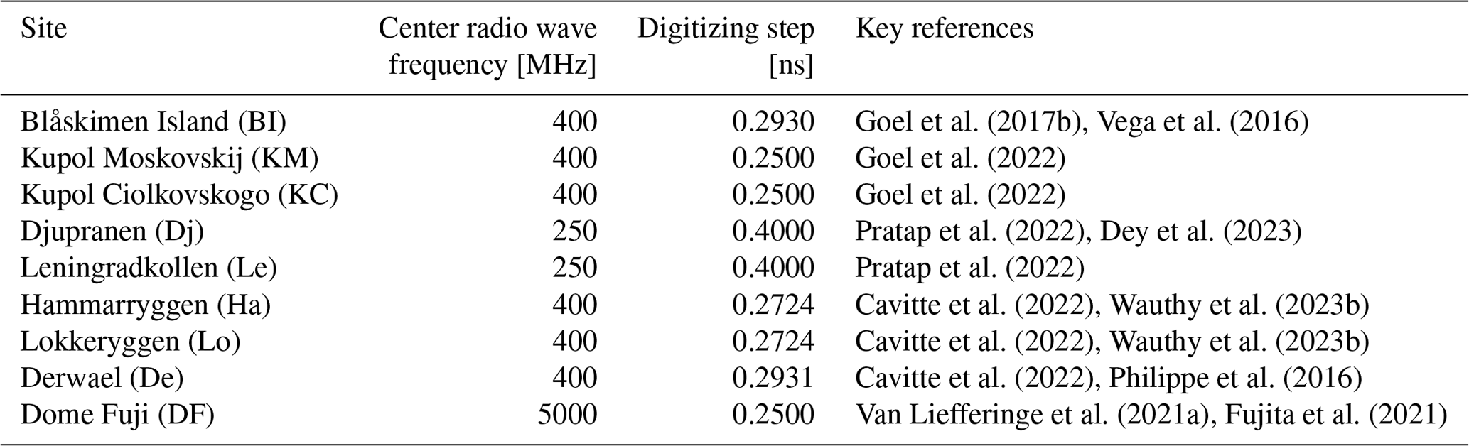
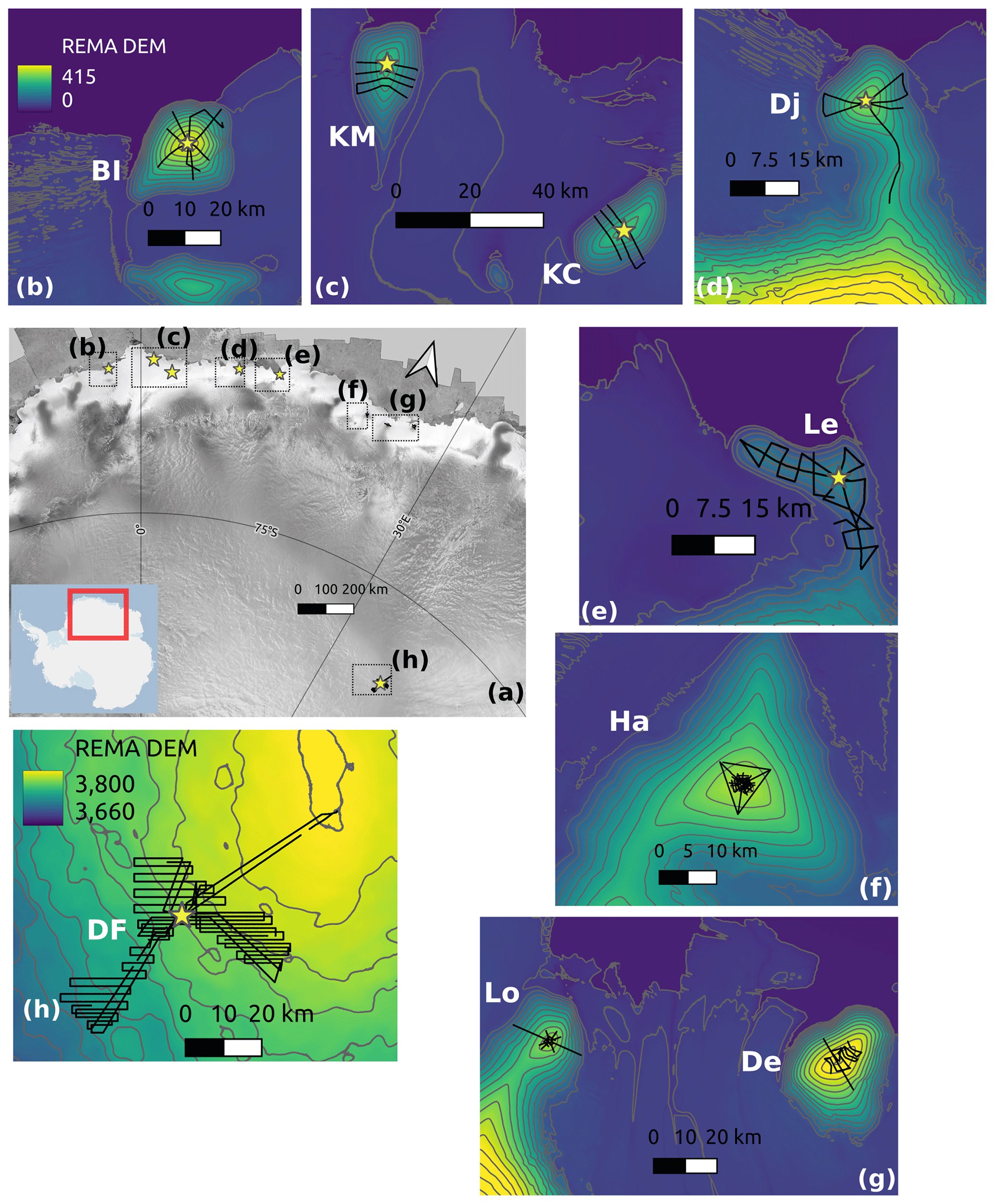
Figure 1Basemaps of the individual study sites which comprise the eight coastal ice rises and the interior dome. Ice cores and radar surveys used in this study are highlighted as yellow stars and black lines, respectively. (a) General view of all sites with the RAMP RADARSAT mosaic (Jezek et al., 2013) as the background, with the inset showing the RAMP mosaic area. (b–h) Zoomed-in view of the individual radar surveys and co-located ice cores. The sites' initials used in all other figures are provided on each panel: BI is Blåskimen Island, KM is Kupol Moskovskij, KC is Kupol Ciolkovskogo, Dj is Djupranen, Le is Leningradkollen, Ha is Hammarryggen, Lo is Lokkeryggen, De is Derwael and DF is Dome Fuji. Background is the Reference Elevation Model of Antarctica (REMA) v2 elevation (units are meters and referenced to the WGS84 ellipsoid); contour lines are shown at 10 m intervals (Howat et al., 2019). Note that the REMA elevation color bounds are the same for panels (b)–(g), while panel (h) has its own bounds. This figure was prepared with Quantarctica (Matsuoka et al., 2021).
The methods used for this work are adapted from the Cavitte et al. (2022) study. We describe them more succinctly here below. We emphasize that to compare SMB measured in the ice cores to that derived from the radar data directly we need to make sure that the SMB records from the ice core and from the radar are at the same temporal resolution, which is why the ice core SMB is calculated per pair of radar IRH depths.
4.1 Ice core SMB
We use the published ice core data, specifically the age, depth and density measurements (Table 1 summarizes the key source data). Using the depth–density raw measurements at each ice core site, we calculate the best-fit depth–density profile between the surface and the deepest radar IRH depth considered, as done previously in Cavitte et al. (2022) (Fig. S1 in the Supplement). For the coastal sites, we use the exponential function of depth versus density by Hubbard et al. (2013), developed for the Derwael ice core. We adjust this exponential function for each ice core site so that the highest R2 value (coefficient of determination; see Sect. S1 in the Supplement) is obtained for the fit between the raw ice core density measurements and the exponential curve. The R2 values obtained vary from 0.63 at Leningradkollen to 0.99 at Lokkeryggen and Hammarryggen (see Sect. S1). Note that applying a Herron–Langway depth–density fit (Herron and Langway, 1980), as applied for the radar-derived data, gives the same R2 values (within ±0.02) as the R2 exponential fits. This implies that the ice core density exponential fits and radar-derived Herron–Langway density fits are relatively similar. For the Dome Fuji region, we use the linear best fit outlined by Van Liefferinge et al. (2021a), measured across four shallow cores collected down to 20 m depth in the Dome Fuji area. The best-fit equations obtained at each site are provided in Sect. S1 as well as the profiles (Fig. S1). Next, we integrate the best-fit density profile with respect to depth to obtain the cumulative mass as a function of depth in each ice core. Equations linking cumulative mass and depth are also provided for each site in Sect. S1. We calculate cumulative mass between the surface and the depth of each IRH, CM. This allows us to compare the radar and ice core SMB records easily. The mean SMB for each time interval contained between successive pairs of IRHs at the ice core location (where the density profile is known) is obtained by dividing the difference between the deepest and the shallowest CMIRH of successive IRHs by the time interval contained between the pairs of dated IRHs. We note that we use the updated Dey et al. (2023) chronology for the Djupranen ice core.
4.2 Radar-derived SMB
4.2.1 Calculating SMB from the IRH data
In summary, we use the published IRH TWTTs and the co-located ice core chronologies to obtain best-fit density profiles, allowing us to calculate a SMB record at each radar data point. This ensures that the SMB rates are calculated from the radar data consistently across all of the sites studied. Note that this is why the ages of the IRHs and the SMB history reconstructed from the radar differ slightly from previously published studies. We refer readers to Cavitte et al. (2022) for more details about our method. Table 2 provides a summary of the radar IRH data sets used.
Many studies assume horizontal homogeneity of the surface density, often done because only one surface density is measured during a radar campaign, that of the central ice core. However, we know that surface density is highly variable, especially in coastal areas. Wever et al. (2022) have shown that snow events can exhibit up to 150 kg m−3 of differences in density at the Hammarryggen ice rise. Matsuoka et al. (2015) have shown that there is a 35 % spatial density variation over three ice rises in the Fimbul Ice Shelf, while Goel et al. (2022) describe surface density variations of ±2.5 % over Blåskimen Island, ±7 % over Kupol Moskovskij and ±2.5 % over Kupol Ciolkovskogo. Therefore, we calculate a density profile at every radar data point, based on fitting the IRH geometries and matching the IRH ages, which allows us to calculate a SMB history. The first step is to date the IRHs. The ice core best-fit density profile described above is used to convert the IRH TWTT to depth at the point of closest distance to the ice core site, where we have a measured density profile. Each IRH depth obtained can then be matched to an ice core depth, and each IRH can therefore be dated by linear interpolation of the ice core age–depth timescale. IRHs have different spatial extents depending on their brightness and continuity and so the point closest to the ice core site might vary with the depth of the IRH considered. This is why we report a range of the shortest distances between the IRHs and the ice core sites for some locations in Table 2. Note that the Derwael ice rise site is an exception: the IRH age is the mean age over three locations intersecting the Raymond arch (Cavitte et al., 2022).
The next step is to convert the IRH TWTTs and ages into a SMB history for every radar data point at each site. As stated earlier, density varies a lot in the near surface. Therefore, we use an adaptation of the Medley et al. (2013) algorithm that allows us to invert the IRH ages and TWTTs to obtain a long-term SMB record with depth (SMB calculated between the surface and each IRH) at each radar data point. We apply the Herron and Langway (Herron and Langway, 1980) depth–density profile, using initial guesses for mean surface temperature and mean SMB from RACMO2.3p2 (van Wessem et al., 2018) over 1979–2016 and surface density from the co-located ice core. This density profile is then converted into a cumulated mass from the surface. Combined with the IRH age information, a first long-term SMB record is obtained. This long-term SMB record is compared to the initial-guess SMB. As long as the difference obtained between the prior SMB record and the resulting SMB record is larger than 0.1 mm w.e. yr−1 for all time intervals, we iterate using the previous long-term SMB history as an initial guess. Once the difference in long-term SMB history between two iterations is within 0.01 mm w.e. yr−1 for all IRH pairs (which usually takes approximately four to five iterations), we consider that we have obtained the best estimate of the long-term SMB history. We can then obtain the mean SMB between pairs of IRHs (i.e., what we refer to as the radar-derived SMB) by dividing the long-term SMB history by the time interval contained between the pairs of IRH for each radar data point.
We would like to highlight that the ages of the IRHs over the Lokkeryggen and Hammarryggen ice rises are from the newly published ice core (Wauthy et al., 2023b) chronologies, which are changed with respect to the preliminary chronologies used in Cavitte et al. (2022). In addition, note that for the Djupranen site we use the IRH TWTTs as given in the Pratap et al. (2022) and the recent chronology update published by Dey et al. (2023), while based on comparison of mass balance estimates though different approaches (Goel et al., 2022) we highlight that it is suspected that the age chronology of the Kupol Moskovskij ice core might be in error.
Goel et al. (2017b, a)Goel et al. (2017b, a)Goel et al. (2017b, a)Pratap et al. (2022, 2021)Pratap et al. (2022, 2021)Cavitte et al. (2022)Cavitte (2022)Cavitte et al. (2022)Cavitte (2022)Cavitte et al. (2022)Cavitte (2022)Van Liefferinge et al. (2021a, b)Table 2IRH data set sources and main characteristics. Same abbreviations as in Fig. 1.
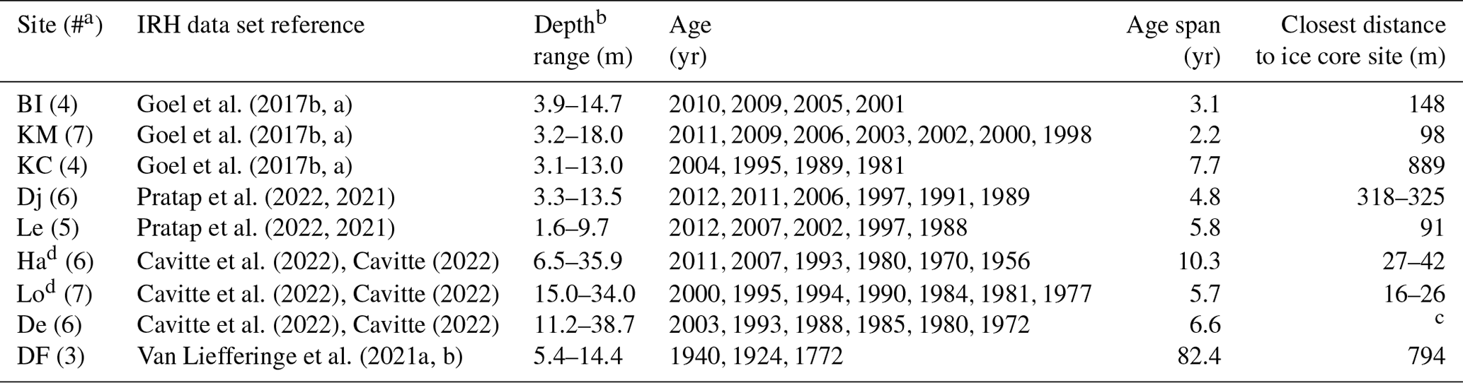
a Brackets indicate the number of isochrones in the radar data set. b Depths are measured at the point of closest approach to the ice core site, except for Derwael, where depths are the average over the three equivalent locations, as described in Sect. 3.1. c The closest distance does not apply to the Derwael ice rise, as described in Sect. 3.1. d Note that IRH ages for the Lokkeryggen and Hammarryggen sites have been updated from those provided in Cavitte et al. (2022), which were based on preliminary ice core chronologies.
4.2.2 Gridding SMB
To quantify the spatial representativeness of the individual point SMB measurements, i.e., the ice-core-measured SMB, we compare them to the radar-derived SMB obtained over a larger surface for each region. However, we have a sampling bias of the radar which is orders of magnitude denser in the along-transect than the across-transect direction (meters versus kilometers, respectively). To minimize the sampling bias of the radar data, we resample the radar survey data onto a regular square grid, as described in Cavitte et al. (2022), for three square grid cell sizes: 50×50, 100×100 and 250×250 m. This smooths out the spatial heterogeneity of the individual radar survey designs. The SMB record of each grid cell is the average of the SMB records for all the radar data points that fall within that grid cell. We compared the mean SMB obtained with and without gridding for the entire survey region. The difference with and without gridding is insignificant for all sites in terms of differences in mean SMB with respect to the SMB uncertainties. It is significant for two ice rise sites in terms of temporal variability (9 % and 11 % increases in temporal variability with the gridded product; see Sect. 4.3 for the uncertainty quantification).
The compiled data sets, namely the gridded radar-derived SMB data are available at https://doi.org/10.14428/DVN/J34MQO (Cavitte, 2023).
4.3 Error analysis
4.3.1 Radar-derived SMB uncertainty
For the radar, the sources of SMB uncertainty are two-fold, related to errors in the densities and the measured IRH TWTT thickness that results from the radar system used to collect the radar data. We quantify the density error as the standard deviation across all the density profiles per radar survey (Fig. S2), following the approach by Medley et al. (2013). This density error affects the SMB calculated by modifying the cumulative mass between IRH pairs. The impact of this mass error is assessed by calculating the SMB between IRH pairs, once using the mean density profile (mean of all density profiles per radar survey) and again using the mean density profile from which we add or subtract the density error. The difference obtained between the SMB derived using the mean densities and the SMB derived using the modified densities (density ± standard deviation of the density) gives us the contribution to the total SMB error as a result of this mass error. This density-related mass error is estimated to have a range between 0 % and 4.6 % across all the radar survey sites (Fig. 2). The density error also affects the calculated SMB by impacting the conversion of the IRHs' TWTT to depth. The impact of this density-related depth error on the calculated SMB history can be assessed in a similar way as above but this time by evaluating the TWTT-to-depth conversion using the mean density profile or modified by the density error. This density-related depth error is estimated to have an impact of up to 2.8 % on the calculated radar-derived SMB across all study sites (Fig. 2). Finally, we assign each IRH a TWTT-thickness uncertainty equal to 4 times the digitization step for each radar data set (Table 1), as we observe the traced radar IRHs to typically be ∼ 4 pixels wide in the TWTT domain. This measured IRH TWTT-thickness uncertainty affects the calculated SMB by impacting the measured TWTT of the radar IRHs. We calculate the SMB between IRH pairs by using the IRH TWTTs modified by ±2 times the digitization step, which we compare to the calculated SMB without IRH TWTT modification. The resulting SMB error is estimated to be between 0.4 % and 6.9 % of the radar-derived SMB across all study sites (Fig. 2). We highlight that the relative significance between the assigned digitizing error (4 pixels) and the TWTT of the IRH (i.e., total number of pixels) has a strong influence on the resulting SMB error magnitude. For example, the Leningradkollen and Djupranen sites have the same digitization step; however, because the IRHs traced over Leningradkollen have shallower depths than those traced over the Djupranen site, the relative SMB error is larger at Leningradkollen than at Djupranen. This is clearly visible in Fig. 2.
We combine these three errors as a root-mean-squared error, resulting in a total radar-derived SMB uncertainty across all sites that varies between a minimum of 0.5 % of the mean radar-derived SMB for the interval between the surface and the shallowest IRH at Lo and a maximum of 6.9 % of the mean radar-derived SMB for the interval between the two deepest IRHs at each site at Leningradkollen (Fig. 2). Because SMB is evaluated as a cumulative mass from the surface, SMB uncertainties increase with depth (and age) of the IRHs. If we average the total radar-derived SMB uncertainty across all sites, we get a mean radar-derived SMB uncertainty of 1.9 % near the surface and 3.5 % for the deepest IRHs. Detailed site-by-site SMB uncertainties are provided in Sect. S3 (Table S1 in the Supplement).
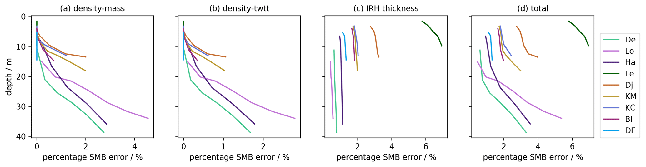
Figure 2Radar-derived SMB uncertainty due to (a) density-related mass error, (b) density-related TWTT error, (c) measured IRH TWTT thickness and (d) combined SMB uncertainty. Each studied region is indicated by a different color. SMB uncertainty increases with depth, as SMB is calculated with respect to a cumulative mass between time markers. Note that the density-related mass error and the density-related TWTT error are the same for Leningradkollen and Djupranen and so the two curves overlay each other. Abbreviations are the same as shown in Fig. 1.
4.3.2 Ice core SMB uncertainty
For the ice core, the sources of SMB uncertainty are two-fold, related to the error made in estimating a best fit from the raw density measurements and to the accuracy in measuring the individual ice core section lengths during drilling operations. Since we are comparing ice core and radar-derived SMB, the age scale applied is identical, and we can ignore the ice core dating uncertainty. We quantify the density-related error by calculating the standard deviation error between the ice core raw-measured densities and the exponential fit of the densities at each site. We note that this calculated density error matches that of the ice core density measurement errors where reported (Hubbard et al., 2013; Pratap et al., 2022; Dey et al., 2023). We then evaluate the impact of this density error on the calculation of the ice core SMB. The total SMB error is determined as the difference between the SMB obtained using the best-fit density profile and the SMB obtained using the best-fit density profile ± the density error. This is assessed by calculating the cumulative mass to each ice core depth marker, using the three density profiles determined. This cumulative mass is then interpolated to obtain the cumulative mass to each IRH depth, which we divide by the time interval contained between IRH pairs as before. This density-related mass error is estimated between 1.3 % and 8.5 % of the ice core SMB across all survey sites, except for the NDFN ice core, where this error varies between 13.7 %–16 % of the ice core SMB (Fig. 3). This larger relative error for NDFN is due to the fact that the absolute snow accumulation rates are a factor of 100 smaller than at the coastal sites and so a small mass error corresponds to a large relative SMB error. Note that the exponential fit is often worse near the surface (Fig. S1) and so the SMB uncertainty related to this density error is largest near the surface and decreases with depth for all regions studied. Figure 3a shows this inverted relationship well. Second, we evaluate the depth error due to core length measurement error. This depth error is rarely reported in publications in general because of its negligible impact versus errors made in the dating of the ice. Since it is not reported for the ice core data sets used, we make the assumption that a 1 mm measurement error is made for every 0.5 m of ice core drilled, for all ice core sites considered in this study, which accumulates with depth. A depth error is then assigned to each IRH depth, and we calculate the SMB using the exponential functions described in Sect. 3.1, once for the IRH depth and then for the IRH depth ± half of the IRH-assigned depth error. This results in an ice core SMB error of around 0.1 %, including at NDFN. This depth-related SMB error is 10 times smaller than then density-related SMB error and can therefore be ignored. The total ice core SMB error is therefore equal to the density-related error (Fig. 3).
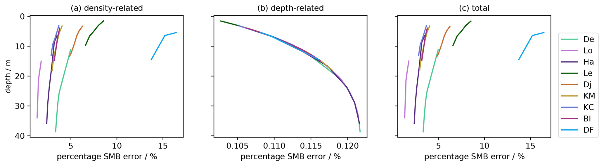
Figure 3Ice core SMB uncertainty due to (a) density-related SMB error, (b) depth-related SMB error and (c) combined total SMB uncertainty; each study site is portrayed by a different color. SMB uncertainty decreases with depth due to the improved fit of the exponential density profile away from the surface. Abbreviations are the same as shown in Fig. 1.
We observe that the ice core SMB uncertainties are largest at the surface due to the larger number of measurement outliers near the surface and where the exponential profile is less adapted. The SMB error is largest for the NDFN core, as the misfit between the linear profile and the measurement points is strongest, enhanced by the low SMB absolute values. The SMB error decreases with depth, with an increasing fit of the exponential profile to the measurements (Sect. S1, Fig. S1). Detailed site-by-site SMB uncertainties are provided in Sect. S3 (Table S2).
5.1 Spatial patterns of SMB
5.1.1 Coastal ice rises
All ice rise sites show a clear east–west spatial pattern with higher SMB values on the eastward side and lower SMB values on the westward side of the ice rise crests. With the dominating east-to-west wind patterns, the eastward side of the ice rise corresponds to the windward side and the westward side to the leeward side. The ratio of the mean windward SMB to the mean leeward SMB varies between 1.1 at Lokkeryggen and 2.3 at Kupol Ciolkovskogo, with the exception of Djupranen, whose ratio is 1, perhaps linked to the survey design which is uniformly split into sampling the windward and leeward slopes of the ice rise (Fig. S5 in the Supplement). Blåskimen Island ice rise is shown as an example in Fig. 4, and all the other sites can be found in Sect. S4. We note that Leningradkollen ice rise shows a less clear east–west pattern. Instead, it shows higher values on the southern side of the east–west ridge and in the saddle between the seaward and the landward ridges, already described in Pratap et al. (2022). SMB values vary between 10 and 150 cm w.e. yr−1 across all coastal ice rise sites, and the spatial patterns of SMB remain relatively stationary over the different time intervals. Note that the absolute values of SMB at Lokkeryggen and Hammarryggen are significantly different from the Cavitte et al. (2022) study as a result of the updated ice core chronologies as mentioned above. We do not go into more detail on the spatio-temporal patterns of SMB at each site, as these are described at length in the source data set publications (Pratap et al., 2022; Goel et al., 2017b, 2022; Cavitte et al., 2022).
5.1.2 Dome Fuji
The interior Dome Fuji site shows a factor of 10 lower SMB rates than over the coastal ice rises, ranging between 1 and 2.5 cm w.e. yr−1, with a very heterogeneous SMB spatial pattern – no clear east–west pattern – that is stationary over all three time intervals. Van Liefferinge et al. (2021a) describe the spatial distribution of SMB more at length.
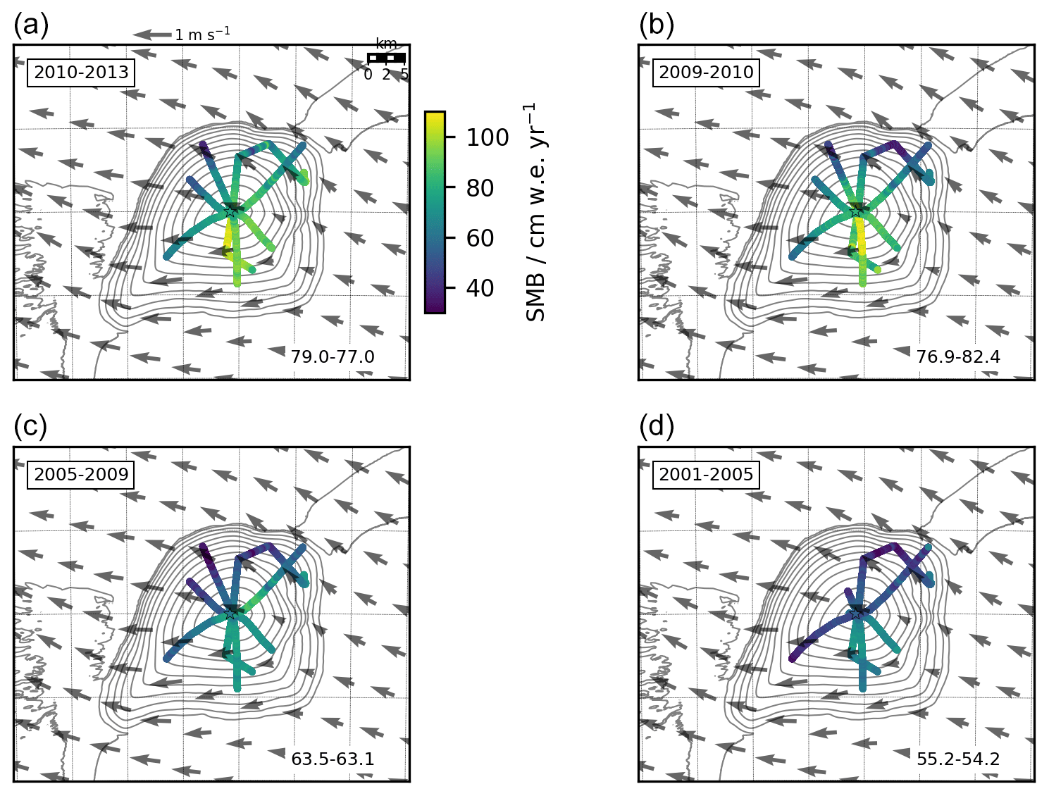
Figure 4Spatial distribution of SMB through time at Blåskimen Island. Each panel represents a different time interval, going from most recent in panel (a) to the oldest in panel (d); the time intervals are provided in the top left corner of each frame. Contours are REMA v2.0 elevation contours, with a 30 m interval; the gray arrows show the mean wind direction (RACMO2.3 5.5 km simulations over 1979–2017, Lenaerts et al., 2017; van Wessem et al., 2018). The wind magnitude scale is shown on the top of the first panel. The numbers in the lower right corner of each panel are radar area average SMB followed by ice core SMB in cm w.e. yr−1.
5.2 Temporal changes of region-mean SMB
5.2.1 Coastal ice rises
From the Blåskimen Island ice rise example in Fig. 4, we can see that, as we move away from the ice core location, SMB varies greatly on the kilometer scale. To compare the ice core SMB measurements to the SMB derived over a wider area more systematically, we calculate the spatial mean of the radar-derived SMB over the entire radar survey for each site, as done previously in Cavitte et al. (2022). Figure 5 shows the resulting SMB histories for each site examined. The first thing to note is that in all cases SMB from the ice cores is smaller than the regional mean, except to a degree at the Blåskimen Island site. The mean difference between the local and the regional SMB signals, given as the Δμt value at the top of each panel on Fig. 5, varies significantly between sites. At Blåskimen Island, the mean difference is quasi null, while it reaches up to ∼ 24 cm w.e. yr−1 at the Djupranen site, corresponding to 85 % of the Djupranen ice core's SMB temporal mean.
Secondly, it is interesting to note that the SMB temporal evolutions of the point measurement and of the area average are very similar for some sites (e.g., this is particularly the case for the Hammarryggen, Lokkeryggen and Derwael sites) and less so for other sites (e.g., Kupol Moskovskij, Djupranen and Leningradkollen sites; Fig. 5). Combining ice core and radar measurements allows us to estimate the uncertainty in measuring SMB locally (Δobst) for the surface area sampled by the radar survey. We estimate the uncertainty in measuring SMB locally (Δobst) by quantifying the amplitude of the difference between the point measurement and the area average at each site (after removing the mean SMB bias between the two proxies). In practice, we define Δobst as the standard deviation of the difference between the ice core and the radar-derived SMB anomalies (i.e., SMB record minus its temporal mean) at each site. Δobst is given at the top of each panel in Fig. 5 (equations in Sect. S5). We then normalize Δobst by the ice core SMB temporal variability, differing from the method used in Cavitte et al. (2022), where Δobst (%) was given relative to the ice core mean SMB. Δobst (%) is therefore the relative uncertainty in the SMB temporal variability, i.e., the ratio of the uncertainty in the SMB temporal variability to the SMB temporal variability. Δobst (%) varies greatly from site to site, reaching from a maximum of 180 % over the Kupol Moskovskij ice rise down to 26 % at Blåskimen Island. In the definition of the relative uncertainty in the SMB temporal variability Δobst (%) given here, a value of 100 % or above implies that the signal uncertainty is equivalent to or larger than the local signal strength. It corresponds to four ice rise sites in our sample: Kupol Moskovskij, Djupranen, Leningradkollen and Lokkeryggen. For these four ice rises, the SMB signal strength is weaker than the regional noise brought in from the spatial variability of the SMB.
5.2.2 Dome Fuji
The Dome Fuji site is different from the coastal ice rise sites due to the extremely low accumulation rates observed at this site and the large SMB uncertainties relative to the absolute SMB rates. At Dome Fuji, the point measurement and spatially averaged SMB histories are very similar in terms of trend and temporal mean. The mean difference is quasi null (3 % of the ice core mean SMB) and clearly much smaller than the SMB uncertainties calculated for the ice core SMB record (Fig. 5). The Dome Fuji ice core shows a relative uncertainty in the SMB temporal variability (Δobst) (%) of 55 %, which implies that the local SMB signal strength is above the SMB noise.
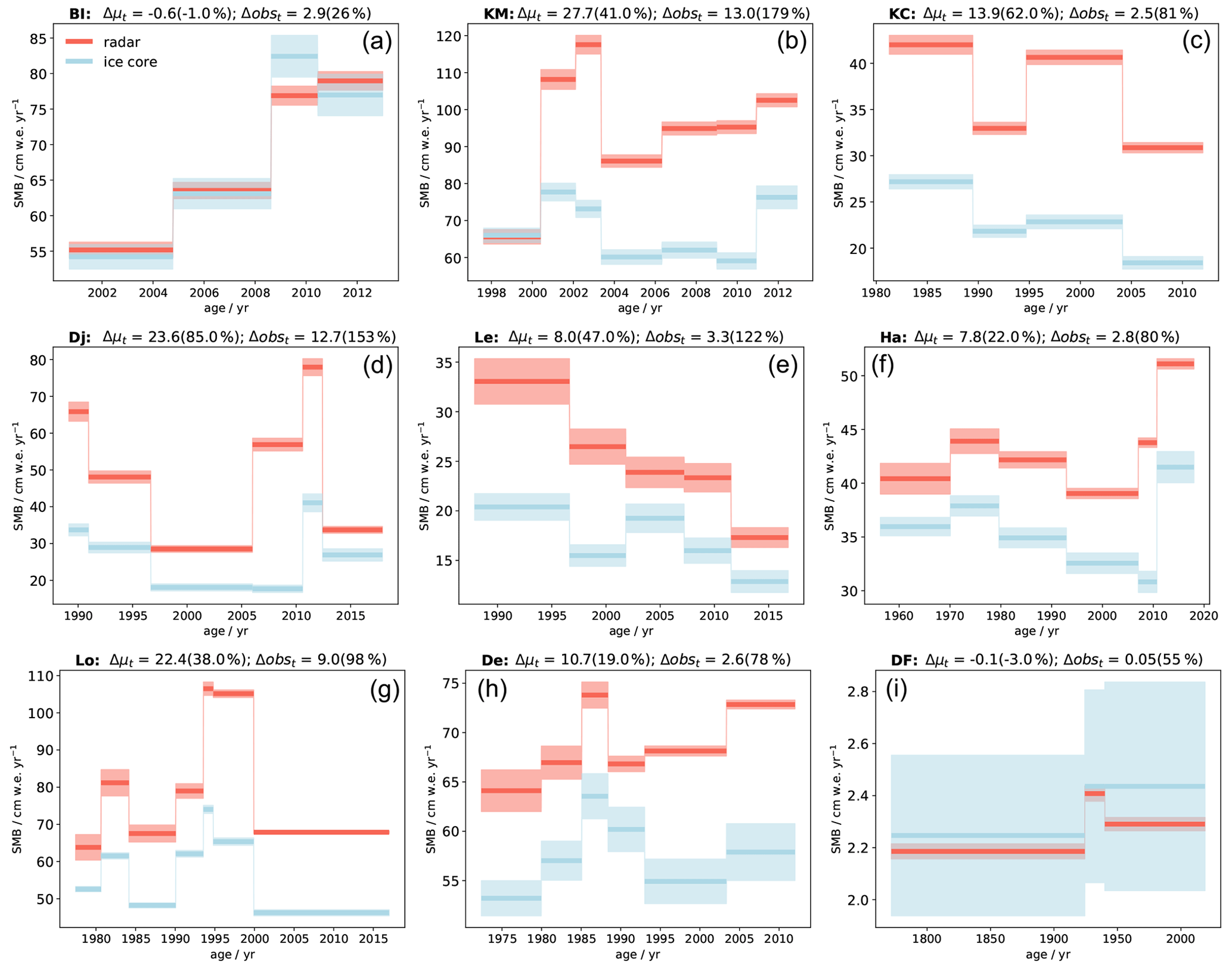
Figure 5Ice core (blue) vs. regional (radar spatial average, red) SMB history, with the calculated SMB uncertainties as blue and red bands, respectively (legend is provided in panel a). Sites are labeled at the top of each panel and are ordered left to right from the westernmost coastal site to the easternmost coastal site, and the Dome Fuji site is last. On top of each panel, Δμt indicates the difference in the mean SMB between the two SMB series in cm w.e. yr−1, with the difference given as a percentage of the ice core mean SMB in brackets. Δobst indicates the uncertainty in measuring SMB locally between two SMB series in cm w.e. yr−1, with relative uncertainty as a percentage value in brackets (normalized to the standard deviation of the ice core SMB anomaly around the temporal mean).
5.3 Spatial representativeness of ice-core-derived SMB
5.3.1 Coastal ice rises
We note that comparing the radar spatially averaged SMB to the measured ice core SMB in terms of a single mean SMB value (Fig. 5) is difficult with the varying radar coverage between sites. To quantify the representativeness as a function of distance from the ice core sites across all study regions, we plot the difference in mean and temporal variability (calculated as before) between the ice core SMB and the regional SMB (radar spatial average) for varying surface areas centered on the ice core sites (Figs. 6 and 7). We use the 50 m gridded radar product, but we note that the results are unchanged if the 100 and 250 m grid resolutions are used (see Sect. S6 and Fig. S11). We can see that as the surface area over which the radar spatial average is calculated increases the mean SMB difference between the point measurement and the area average increases rapidly too. For the Kupol Moskovskij, Lokkeryggen, Hammarryggen and Derwael sites, the difference in the mean SMB seems to plateau for a surface area of ∼ 8 km2, at which point the mean differences reach a maximum of between 20 % and 40 % of the ice core mean SMB. At the Kupol Ciolkovskogo, Leningradkollen and Djupranen sites, the difference in mean SMB continues to grow with increasing surface areas and only stabilizes for a surface area ∼ 300 km2, and the difference between the ice core SMB and the spatially averaged SMB reaches between 50 % and 85 % of the ice core mean SMB. At the Blåskimen Island ice rise, the difference in mean SMB between ice core and area average increases with surface area but remains low, below 5 % of the ice core mean SMB for all surface areas considered. Regarding the relative uncertainty in measuring SMB locally (Δobst) (%) for the surface area sampled by the radar survey, we see that this uncertainty increases rapidly for all ice rise sites (except BI), stabilizing below 100 % for the Lokkeryggen, Kupol Ciolkovskogo, Hammarryggen and Derwael sites, while for the Leningradkollen, Djupranen and Kupol Moskovskij sites the 100 % threshold is crossed for surface areas varying between 20 and 120 km2 and plateaus out at a relative SMB uncertainty equal to 125 %–175 % of the temporal variability of the ice core SMB signal. The Blåskimen Island ice rise site stands out with a very low relative SMB uncertainty (Δobst) (%), remaining at around 25 % of the ice core SMB signal for all surface areas considered. This implies that at Lokkeryggen, Kupol Ciolkovskogo, Hammarryggen, Derwael and particularly Blåskimen Island the signal strength is higher than the noise introduced by the spatial variability of the SMB signal, and the inverse is true for the Leningradkollen, Djupranen and Kupol Moskovskij sites.
5.3.2 Dome Fuji
At the Dome Fuji plateau site, the difference in mean SMB between ice core and area average increases with surface area but remains low and negative, between −3 % and 0 % of the ice core mean SMB for all surface areas considered, which implies that the ice-core-measured SMB is generally higher than that of the area average. In terms of relative uncertainty in measuring SMB locally (Δobst) (%), the plateau Dome Fuji site shows an opposite trend to the ice rises, with a maximum value when the smallest surface area is considered (∼ 200 % of the temporal variability of the ice core SMB signal) and a plateau-out of ∼ 100 % for a surface area at ∼ 300 km2.
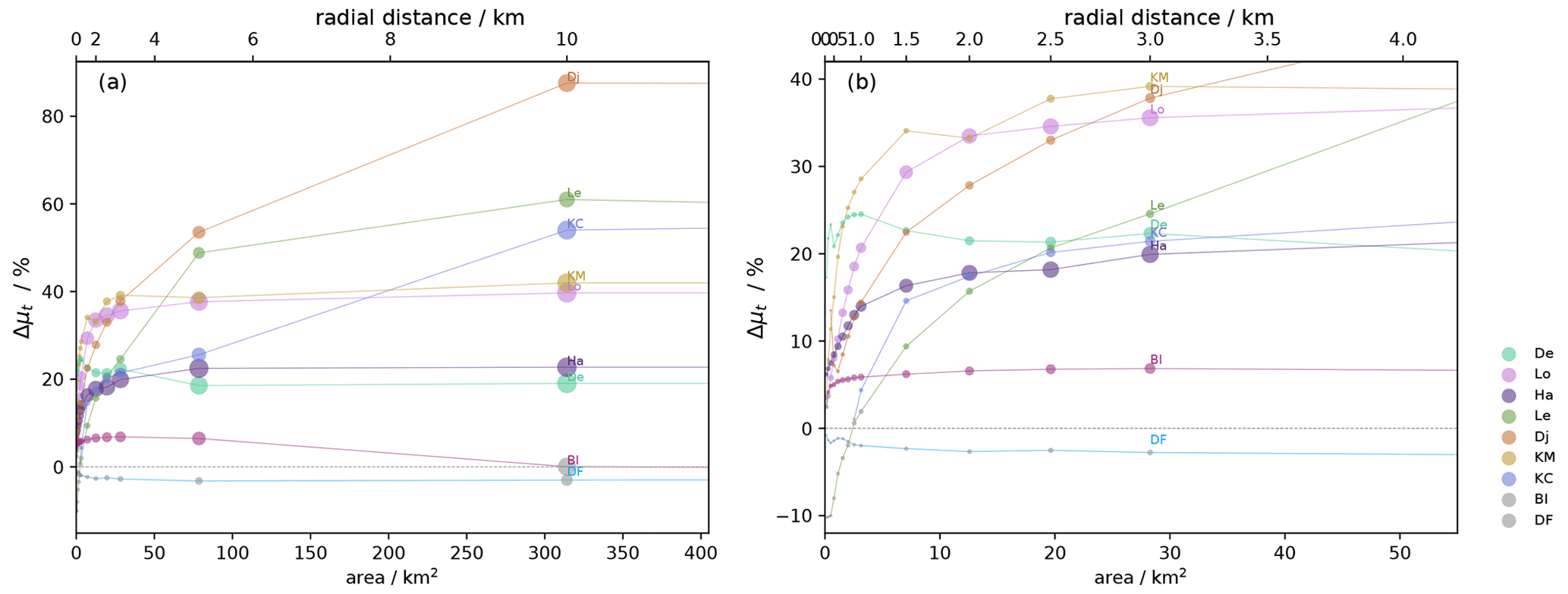
Figure 6Relative difference (%) in mean SMB value between gridded radar-derived SMB (at 50 m spatial resolution) and ice core SMB as a function of surface area. Panel (b) focuses on surface areas up to 50 km2 around the ice core site. Each site is represented by a different color; the gray dots imply that the difference is negligible with respect to the SMB uncertainties. The size of the dots represents the number of grid points within the radial distance.
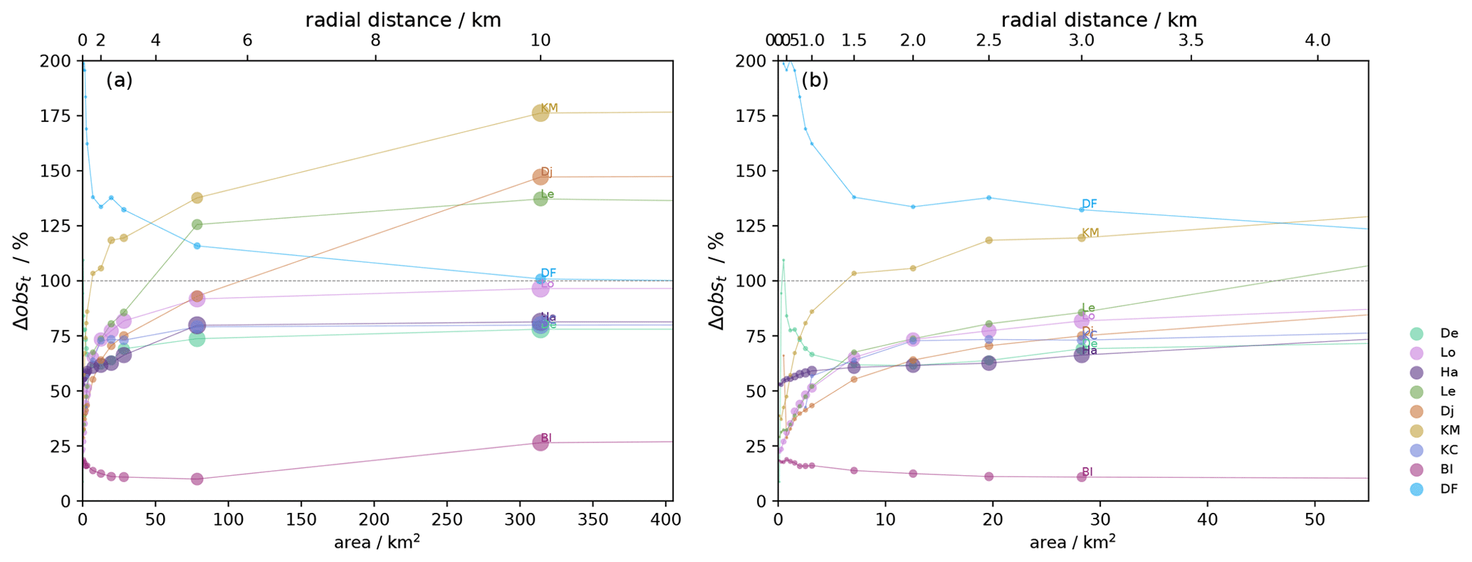
Figure 7Relative uncertainty in measuring SMB locally (Δobst) (%). Panel (b) focuses on surface areas up to 50 km2 around the ice core site. Each site is represented by a different color; the gray dots imply that the difference is negligible with respect to the SMB uncertainties. The size of the dots represents the number of grid points within the radial distance.
Cavitte et al. (2022) have shown that for the Derwael, Lokkeryggen and Hammarryggen ice rises the spatial representativeness of the ice cores in terms of mean SMB was limited to a distance ∼ 200–500 m away from the ice core site. This conclusion was based on the criterion that the difference between the local and the regional signals became smaller than the SMB uncertainties measured. That study showed, therefore, that beyond 500 m the ice core mean value always underestimated the regional mean, which could be adjusted based on the regional mean to be representative of a wider region. With the addition of five ice rise sites and an interior plateau site, we observe here that the ice cores' representativeness varies widely from site to site. Considering the difference in mean SMB between a point measurement of SMB and the wider area average, as in Fig. 6, it is clear that these differences cannot be explained through a simple relationship such as distance away from the ice core site. We note that at all ice rise sites the mean difference in SMB between a point measurement of SMB and the wider area average increases with the size of the surface area considered. However, the rate at which this difference increases varies from site to site. Since our highest calculated uncertainty is ∼ 8 % of the SMB signal for both the ice core and the radar, we describe the representativeness of point measurements using the threshold of a 10 % difference in mean SMB between the local and the regional signals, as opposed to the uncertainty value threshold as in Cavitte et al. (2022). This allows us to explicitly recognize that ice cores' representativeness exists on a continuous spectrum and to ensure that the results are not dependent on the quality of the data (i.e., higher-quality radar or ice core data could decrease the error and therefore influence the determined representativeness).
The difference in mean SMB increases beyond 10 % of the ice core mean SMB for a surface area that varies between a minimum of ∼ 0.4 km2 at Kupol Moskovskij and a maximum of 9.6 km2 at Leningradkollen. It is interesting that for five of the ice rise sites the difference in the mean SMB plateaus for a surface of around ∼ 8 km2, which corresponds to ∼ 1–2 km away from the ice rise crests. This is the typical distance over which a dome and crest SMB pattern is observed over the ice rises (Kausch et al., 2020; Goel et al., 2022) and so this plateau could be linked to the depositional and erosional SMB regimes near the ice rises' summits. The second plateau is reached by the Kupol Ciolkovskogo, Leningradkollen and Djupranen sites for a surface area of ∼ 300 km2, corresponding to ∼ 10 km away from the ice rise crests, which is typically the distance where the orographic SMB regime of the ice rises meets the flat ice shelves. For Blåskimen Island and Dome Fuji, the mean difference remains below 10 % of the ice core mean SMB for all surface areas considered. This suggests that both ice cores have a good representativeness of the larger region. On the other end of the spectrum, the Djupranen and Leningradkollen ice cores record the most local SMB signal, with a difference in mean SMB between the point measurement and the regional mean increasing rapidly, up to 90 % and ∼ 60 %, respectively, of the ice core mean SMB for a surface area of 300 km2. If we consider that regional climate models often have a spatial resolution on the order of 25 km × 25 km (625 km2), this has important implications for the use of ice cores as model simulation validations. As previously suggested in Cavitte et al. (2022), an option would be to shift the mean SMB value of the ice core series based on the assessed difference in mean SMB with a co-located radar-derived SMB series.
Cavitte et al. (2022) had also shown that the SMB temporal variability tends to be mirrored between the ice core measurements and the radar-derived average SMB for the Hammarryggen, Lokkeryggen and Derwael sites, also visible here in Fig. 5. In this extended study, we estimate the uncertainty in measuring SMB locally (Δobst) to represent a certain surface area and show that for most ice rise sites this uncertainty increases rapidly as the size of the surface area considered increases. Considering the relative uncertainty (Δobst) (%) (i.e., normalized to the ice core's SMB temporal variability), five ice rises out of the eight (Lokkeryggen, Kupol Ciolkovskogo, Hammarryggen, Derwael and Blåskimen Island) show a Δobst (%) that remains below 100 % of the ice core temporal variability. This suggests that the ice cores sample a temporal variability signal that is relatively strong and representative of a relatively large surface area. We note the very low Δobst (%) value at the Blåskimen Island ice rise, implying that the ice core has the highest reliability in sampling the temporal variability of the area. For the Dome Fuji area, the interpretation of Δobst might be limited by the fact that only three time intervals are available to calculate the temporal variability of the signal and that the SMB rates are so low (on the order of a few centimeters of water equivalent per year) that even small errors in the radar-derived SMB from the iterations or the density best fit for the ice core SMB will have a very large impact on the final differences obtained. For the Kupol Moskovskij, Djupranen and Leningradkollen ice rises, the difference increases beyond 100 % of the ice core temporal variability, which implies that they record a more noisy record of SMB temporal variability. A 100 % difference in temporal variability is reached between a surface area of ∼ 20 km2 for Kupol Moskovskij, ∼ 50 km2 for Leningradkollen and ∼ 120 km2 for Djupranen. It is interesting to note that the Djupranen and Leningradkollen ice rises are two adjacent sites, in the Nivlisen Ice Shelf, where SMB ice core estimates are on the less representative end in terms of both mean and temporal variability of the SMB of the wider area.
If we, again, take the comparison to a typical regional climate model resolution of 25 km × 25 km, our results suggest that the ice cores studied here contain the temporal variability of the SMB signal with varying degrees of noise. This spatial variability of the SMB temporal variability adds noise in the ice core SMB records which cannot be easily corrected by a shift as for the mean SMB representativeness. We suggest that these estimates of the uncertainty in measuring SMB locally to represent a specific surface area could be included in the models. This would ensure that we take into account the uncertainty linked to the spatial variability of the SMB regionally, assessed on the difference in temporal variability with co-located radar-derived SMB.
We have attempted to find the controlling factors behind the varying representativeness of the ice cores' mean SMB. Several factors could explain the spread in mean SMB representativeness across all sites considered: varying absolute snowfall rates, distance from the coast, wind strength, temporal resolution of the radar isochrones considered, and radar survey sampling of the windward and leeward sides (Goel et al., 2017b; Cavitte et al., 2020; Kausch et al., 2020; Pratap et al., 2022; Goel et al., 2022). We have made a preliminary analysis of the influence of each factor individually (see Sect. S6 and Fig. S12), but no single factor explains the spread observed in mean SMB representativeness. It is most likely a combination of several factors that can explain the varying representativeness.
We recognize that one limitation of our study is the differing survey designs at each site which unequally sample the windward and leeward sides of the ice rises. It has been shown previously that the windward side of an ice rise receives more accumulation than the leeward side which is more erosional (Kausch et al., 2020; Goel et al., 2022). A heterogeneous sampling could induce a radar measurement bias that would result in a bias in the ice core–radar differences calculated. To determine the impact of the surveys' sampling, we use the 50 m gridded radar product to calculate the SMB mean over the windward and leeward grid points (east and west side of the ice rises' crests, respectively), which are then averaged together to compare to the SMB mean obtained previously (i.e., calculated over the whole radar area at once). We calculated that the heterogeneous sampling of the ice rises due to the survey designs here induces a bias in the mean SMB, with a minimum of 0.3 % of the mean SMB at Derwael and Kupol Moskovskij and a maximum of 8 % of the mean SMB at Leningradkollen. This falls within the radar-derived SMB uncertainties (Table S1) for all rises except two (Leningradkollen and Kupol Ciolkovskogo) and can therefore be ignored. For Leningradkollen, we do not attempt to correct the bias due to the difficulty in determining the windward and leeward slopes as a result of the ice rise's geometry with respect to the dominant wind direction. As for Kupol Ciolkovskogo, this can be explained due to the larger disparity in radar sampling on the windward versus leeward sides of the ice rise.
If we look at the high plateau site of Dome Fuji individually, we note that it shows very small, albeit negative (the ice core mean SMB is higher than the area average), differences in mean SMB for all surface areas considered, varying between −3 % and −0.8 % of the ice core mean SMB. At this site, the SMB rate is very low, around 1–2.5 cm w.e. yr−1, and precipitation falls 40 % of the time in the form of diamond dust (Dittmann et al., 2016). It has been demonstrated that wind-induced erosion and redeposition have a very large impact on SMB distribution (Frezzotti et al., 2004; Lenaerts et al., 2014, 2019; Kausch et al., 2020). The Dome Fuji site is located in the interior, where surface wind speeds are low (Fig. S10); therefore, we could suppose that the wind-induced redeposition is very limited at Dome Fuji. There is significant spatial variability of SMB, which varies between 1.5–2.5 cm w.e. yr−1 for a single time interval, on the same order of magnitude as the SMB accumulation over the time interval, which Van Liefferinge et al. (2021a) have shown is linked to fine-scale surface topography.
SMB is obtained from radar surveys over eight coastal ice rises and one interior plateau site, which can then be compared to the ice-core-measured SMB for each site. We have shown that we can use the radar-derived SMB to estimate the spatial representativeness of single ice core SMB records. Based on our results, we conclude that the temporal mean SMB measured in ice cores is representative of varying surface areas and does not depend linearly on any one meteorological or topographical factor. We do highlight that there seems to be a link between the spatial variability of the SMB and the controlling factor for the SMB regime (crest–wind interactions versus shelf-to-ice-rise orographic interactions). For a mean difference of 10 % between ice core and radar-derived SMB, ice core SMB is representative of surfaces between 0.5 and 10 km2, corresponding to radial distances < 1 km away from the ice core site. For our westernmost coastal site (Blåskimen Island) and our interior Dome Fuji site, however, the mean difference between ice core and radar-derived SMB always remains below 10 %. Examining the spatial representativeness of the ice cores' SMB temporal variability signal, we showed that the relative uncertainty in measuring SMB locally (Δobst) (%) for the surface area sampled by the radar survey increases rapidly as we move away from the ice core sites. We observed that five of our sites remain below the 100 % threshold for all surface areas considered, implying that their representativeness in terms of temporal variability is relatively strong, while for the other three sites it is limited to a range of between 20–120 km2. Our gridded radar SMB products can be found at https://doi.org/10.14428/DVN/J34MQO (Cavitte, 2023), from which the differences in mean SMB and temporal variability of the SMB signals as a function of distance between the ice cores and the radar-derived data can be recalculated.
All our results tend to indicate that SMB measured in ice cores has a local signature. The Dome Fuji ice core ranks with the highest spatial representativeness, which is consistent with the relatively smooth topography in the region, while Djupranen ranks as having the lowest spatial representativeness. Although RCMs have a relatively high resolution, their grids remain very coarse compared to the spatial footprint of ice cores. High-resolution simulations such as those of RACMO5.5 (Lenaerts et al., 2017; van Wessem et al., 2018) with a grid size of 5.5×5.5 km can be compared directly to ice core SMB if we correct for representativeness, calculated in this study for each site. According to our results, the error of representativeness in mean SMB between the ice core and the area mean over an area of 30 km2 varies between ∼ −3 %–35 % of the ice core mean SMB for the sites we studied here. And for the temporal variability, the error of representativeness varies between ∼ 15 %–130 % of the ice core SMB temporal variability, which could be integrated in a model–ice core comparison.
It would also be interesting to use the radar-derived regional means, over any surface area of interest, to compare directly to model outputs. The radar-derived mean SMB and temporal variability could be calculated for any subset of the radar survey and compared to the model grid cell SMB mean and temporal variability, taking into account the radar-derived SMB uncertainties. This would be complementary to the comparison to ice cores.
As a next step, it will be interesting to compare our derived radar SMB products at each site to RCM SMB simulations, in order to assimilate this new SMB data product in model ensemble simulations. Indeed, data assimilation methods need a well-defined data error prior, which includes measurement uncertainties and the error of representativeness, both detailed in our work.
The Lokkeryggen and Hammarryggen ice cores' full-resolution chronologies and density data are available at https://doi.org/10.5281/Zenodo.7848435 (Wauthy et al., 2023a) and described in full in Wauthy et al. (2023b). The gridded radar-derived SMB calculated for the nine sites for the three different square grid resolutions (250, 100 and 50 m), as well as ages of the radar IRHs are available at https://doi.org/10.14428/DVN/J34MQO (Cavitte, 2023).
The supplement related to this article is available online at: https://doi.org/10.5194/tc-17-4779-2023-supplement.
MGPC led the data analysis and writing. HG and KM provided support in planning the experiments and finalizing the uncertainty quantification. VG, RD, TM, SW and JLT provided ice core age–depth–density data and support regarding the ice core data analysis. VG, BP and BVL provided radar isochrone data and support. BVL provided the statistical analysis for the uncertainty analysis. All co-authors contributed to the discussions on this work. MGPC prepared the paper with contributions from all co-authors.
At least one of the (co-)authors is a member of the editorial board of The Cryosphere. The peer-review process was guided by an independent editor, and the authors also have no other competing interests to declare.
Publisher's note: Copernicus Publications remains neutral with regard to jurisdictional claims made in the text, published maps, institutional affiliations, or any other geographical representation in this paper. While Copernicus Publications makes every effort to include appropriate place names, the final responsibility lies with the authors.
We thank Brooke Medley for her code implementation of the Herron–Langway model, as well as Thore Kausch and Nander Wever for the interesting discussions about surface density. Marie Cavitte is a postdoctoral researcher of the FRS-FNRS. Hugues Goosse is the research director within the FRS-FNRS. Sarah Wauthy has benefited from a FRS-FNRS research fellow grant. This research contributes to the AntArchitecture Action Group of SCAR and partly contributes to the India–Norway collaborative project MADICE to examine mass balance in coastal Dronning Maud Land. Finally, we would like to thank the editor, Joël Savarino, and the referees, Steven Franke and an anonymous reviewer, for their constructive reviews and helpful comments on this paper.
This work was partially supported by the Belgian Research Action through Interdisciplinary Networks (BRAIN-be) from the Belgian Science Policy Office in the framework of the project “East Antarctic surface mass balance in the Anthropocene: observations and multiscale modelling (Mass2Ant)” (contract no. BR/165/A2/Mass2Ant). This work was supported by Marie Cavitte's FRS-FNRS postdoctoral fellowship.
This paper was edited by Joel Savarino and reviewed by Steven Franke and one anonymous referee.
Agosta, C., Amory, C., Kittel, C., Orsi, A., Favier, V., Gallée, H., van den Broeke, M. R., Lenaerts, J. T. M., van Wessem, J. M., van de Berg, W. J., and Fettweis, X.: Estimation of the Antarctic surface mass balance using the regional climate model MAR (1979–2015) and identification of dominant processes, The Cryosphere, 13, 281–296, https://doi.org/10.5194/tc-13-281-2019, 2019. a
Arias, P., Bellouin, N., Coppola, E., Jones, R., Krinner, G., Marotzke, J., Naik, V., Palmer, M., Plattner, G.-K., Rogelj, J., Rojas, M., Sillmann, J., Storelvmo, T., Thorne, P., Trewin, B., Achuta Rao, K., Adhikary, B., Allan, R., Armour, K., Bala, G., Barimalala, R., Berger, S., Canadell, J., Cassou, C., Cherchi, A., Collins, W., Collins, W., Connors, S., Corti, S., Cruz, F., Dentener, F., Dereczynski, C., Di Luca, A., Diongue Niang, A., Doblas-Reyes, F., Dosio, A., Douville, H., Engelbrecht, F., Eyring, V., Fischer, E., Forster, P., Fox-Kemper, B., Fuglestvedt, J., Fyfe, J., Gillett, N., Goldfarb, L., Gorodetskaya, I., Gutierrez, J., Hamdi, R., Hawkins, E., Hewitt, H., Hope, P., Islam, A., Jones, C., Kaufman, D., Kopp, R., Kosaka, Y., Kossin, J., Krakovska, S., Lee, J.-Y., Li, J., Mauritsen, T., Maycock, T., Meinshausen, M., Min, S.-K., Monteiro, P., Ngo-Duc, T., Otto, F., Pinto, I., Pirani, A., Raghavan, K., Ranasinghe, R., Ruane, A., Ruiz, L., Sallée, J.-B., Samset, B., Sathyendranath, S., Seneviratne, S., Sörensson, A., Szopa, S., Takayabu, I., Tréguier, A.-M., van den Hurk, B., Vautard, R., von Schuckmann, K., Zaehle, S., Zhang, X., and Zickfeld, K.: Technical Summary, in: Climate Change 2021 – The Physical Science Basis: Working Group I Contribution to the Sixth Assessment Report of the Intergovernmental Panel on Climate Change, Cambridge University Press, Cambridge, United Kingdom and New York, NY, USA, 33−-144, https://doi.org/10.1017/9781009157896.002, 2021. a
Cavitte, M.: Surface mass balance derived from radar stratigraphy over the past six decades (1956–2018) dated with ice cores over the Derwael Ice Rise, Lokeryggen Ice Rise, and Hammarryggen Ice Rise, Princess Ragnhild Coast, Antarctica, Dataverse UCLouvain [data set], https://doi.org/10.14428/DVN/ZLUGD7, 2022. a, b, c
Cavitte, M.: Gridded surface mass balance derived from shallow radar stratigraphy over eight ice rises along the Dronning Maud Land coast and one site in the Dome Fuji region, Antarctica, Dataverse UCLouvain [data set], https://doi.org/10.14428/DVN/J34MQO, 2023. a, b, c, d
Cavitte, M. G., Goosse, H., Wauthy, S., Kausch, T., Tison, J.-L., Van Liefferinge, B., Pattyn, F., Lenaerts, J. T., and Claeys, P.: From ice core to ground-penetrating radar: representativeness of SMB at three ice rises along the Princess Ragnhild Coast, East Antarctica, J. Glaciol., 68, 1221–1233, https://doi.org/10.1017/jog.2022.39, 2022. a, b, c, d, e, f, g, h, i, j, k, l, m, n, o, p, q, r, s, t, u
Cavitte, M. G. P., Blankenship, D. D., Young, D. A., Schroeder, D. M., Parrenin, F., Lemer, E., MacGregor, J. A., and Siegert, M. J.: Deep radiostratigraphy of the East Antarctic plateau: connecting the Dome C and Vostok ice core sites, J. Glaciol., 62, 323–334, https://doi.org/10.1017/jog.2016.11, 2016. a
Cavitte, M. G. P., Dalaiden, Q., Goosse, H., Lenaerts, J. T. M., and Thomas, E. R.: Reconciling the surface temperature–surface mass balance relationship in models and ice cores in Antarctica over the last 2 centuries, The Cryosphere, 14, 4083–4102, https://doi.org/10.5194/tc-14-4083-2020, 2020. a, b
Clausius, R.: Ueber die bewegende Kraft der Wärme und die Gesetze, welche sich daraus für die Wärmelehre selbst ableiten lassen, Ann. Phys., 155, 500–524, https://doi.org/10.1002/andp.18501550403, 1850. a
CReSIS: CReSIS Radar Depth Sounder Data, https://www.cresis.ku.edu/ (last access: July 2023), 2016. a
Dalaiden, Q., Goosse, H., Klein, F., Lenaerts, J. T. M., Holloway, M., Sime, L., and Thomas, E. R.: How useful is snow accumulation in reconstructing surface air temperature in Antarctica? A study combining ice core records and climate models, The Cryosphere, 14, 1187–1207, https://doi.org/10.5194/tc-14-1187-2020, 2020. a
Dey, R., Thamban, M., Laluraj, C. M., Mahalinganathan, K., Redkar, B. L., Kumar, S., and Matsuoka, K.: Application of visual stratigraphy from line-scan images to constrain chronology and melt features of a firn core from coastal Antarctica, J. Glaciol., 69, 179–190, https://doi.org/10.1017/jog.2022.59, 2023. a, b, c, d
Dittmann, A., Schlosser, E., Masson-Delmotte, V., Powers, J. G., Manning, K. W., Werner, M., and Fujita, K.: Precipitation regime and stable isotopes at Dome Fuji, East Antarctica, Atmos. Chem. Phys., 16, 6883–6900, https://doi.org/10.5194/acp-16-6883-2016, 2016. a, b
Fettweis, X., Franco, B., Tedesco, M., van Angelen, J. H., Lenaerts, J. T. M., van den Broeke, M. R., and Gallée, H.: Estimating the Greenland ice sheet surface mass balance contribution to future sea level rise using the regional atmospheric climate model MAR, The Cryosphere, 7, 469–489, https://doi.org/10.5194/tc-7-469-2013, 2013. a
Frezzotti, M., Pourchet, M., Flora, O., Gandolfi, S., Gay, M., Urbini, S., Vincent, C., Becagli, S., Gragnani, R., Proposito, M., Severi, M., Traversi, R., Udistim, R., and Fily, M.: New estimations of precipitation and surface sublimation in East Antarctica from snow accumulation measurements, Clim. Dynam., 23, 803–813, 2004. a, b
Frezzotti, M., Urbini, S., Proposito, M., Scarchilli, C., and Gandolfi, S.: Spatial and temporal variability of surface mass balance near Talos Dome, East Antarctica, J. Geophys. Res.-Earth, 112, F02032, https://doi.org/10.1029/2006JF000638, 2007. a
Fudge, T. J., Markle, B. R., Cuffey, K. M., Buizert, C., Taylor, K. C., Steig, E. J., Waddington, E. D., Conway, H., and Koutnik, M.: Variable relationship between accumulation and temperature in West Antarctica for the past 31,000 years, Geophys. Res. Lett., 43, 3795–3803, https://doi.org/10.1002/2016GL068356, 2016. a
Fujita, S., Oyabu, I., Kawamura, K., Nakazawa, F., Buizert, C., Liefferinge, B. V., Taylor, D., Tsutaki, S., Gogineni, P., Matsuoka, K., Moholdt, G., Abe-Ouchi, A., Awasthi, A., Gallet, J., Isaksson, E., Motoyama, H., Ohno, H., O'Neill, C., and Pattyn, F.: Antarctic shallow ice cores (NDF, NDFN, DFSE, DFNW) data: Density, chronology, permittivity, DEP, 0–20 m, 1.00, Arctic Data archive System (ADS) [data set], Japan, https://doi.org/10.17592/001.2021102101, 2021. a, b
Goel, V., Brown, J., and Matsuoka, K.: Shallow sounding (400 MHz) radar profiles over three ice rises (Blåskimen Land, Kupol Ciolkovskogo and Kupol Moskovskij) in Western Dronning Maud Land, Norwegian Polar Institute [data set], https://doi.org/10.21334/npolar.2016.925d72c7, 2017a. a, b, c
Goel, V., Brown, J., and Matsuoka, K.: Glaciological settings and recent mass balance of Blåskimen Island in Dronning Maud Land, Antarctica, The Cryosphere, 11, 2883–2896, https://doi.org/10.5194/tc-11-2883-2017, 2017b. a, b, c, d, e, f
Goel, V., Matsuoka, K., Berger, C. D., Lee, I., Dall, J., and Forsberg, R.: Characteristics of ice rises and ice rumples in Dronning Maud Land and Enderby Land, Antarctica, J. Glaciol., 66, 1064–1078, https://doi.org/10.1017/jog.2020.77, 2020. a
Goel, V., Morris, A., Moholdt, G., and Matsuoka, K.: Synthesis of field and satellite data to elucidate recent mass balance of five ice rises in Dronning Maud Land, Antarctica, Front. Earth Sci., 10, 975606, https://doi.org/10.3389/feart.2022.975606, 2022. a, b, c, d, e, f, g, h, i
Gorodetskaya, I. V., Van Lipzig, N. P. M., Van den Broeke, M. R., Mangold, A., Boot, W., and Reijmer, C. H.: Meteorological regimes and accumulation patterns at Utsteinen, Dronning Maud Land, East Antarctica: Analysis of two contrasting years, J. Geophys. Res.-Atmos., 118, 1700–1715, https://doi.org/10.1002/jgrd.50177, 2013. a
Herron, M. M. and Langway, C. C.: Firn Densification: An Empirical Model, J. Glaciol., 25, 373–385, https://doi.org/10.3189/S0022143000015239, 1980. a, b
Hoffmann, H. M., Grieman, M. M., King, A. C. F., Epifanio, J. A., Martin, K., Vladimirova, D., Pryer, H. V., Doyle, E., Schmidt, A., Humby, J. D., Rowell, I. F., Nehrbass-Ahles, C., Thomas, E. R., Mulvaney, R., and Wolff, E. W.: The ST22 chronology for the Skytrain Ice Rise ice core – Part 1: A stratigraphic chronology of the last 2000 years, Clim. Past, 18, 1831–1847, https://doi.org/10.5194/cp-18-1831-2022, 2022. a
Howat, I. M., Porter, C., Smith, B. E., Noh, M.-J., and Morin, P.: The Reference Elevation Model of Antarctica, The Cryosphere, 13, 665–674, https://doi.org/10.5194/tc-13-665-2019, 2019. a
Hubbard, B., Tison, J.-L., Philippe, M., Heene, B., Pattyn, F., Malone, T., and Freitag, J.: Ice shelf density reconstructed from optical televiewer borehole logging, Geophys. Res. Lett., 40, 5882–5887, https://doi.org/10.1002/2013GL058023, 2013. a, b
Jezek, K. C., Curlander, J. C., Carsey, F., Wales, C., and Barry, R. G.: RAMP AMM-1 SAR Image Mosaic of Antarctica, https://nsidc.org/data/nsidc-0103/versions/2 (last access: July 2023), 2013. a
Kausch, T., Lhermitte, S., Lenaerts, J. T. M., Wever, N., Inoue, M., Pattyn, F., Sun, S., Wauthy, S., Tison, J.-L., and van de Berg, W. J.: Impact of coastal East Antarctic ice rises on surface mass balance: insights from observations and modeling, The Cryosphere, 14, 3367–3380, https://doi.org/10.5194/tc-14-3367-2020, 2020. a, b, c, d, e, f
Le Meur, E., Magand, O., Arnaud, L., Fily, M., Frezzotti, M., Cavitte, M., Mulvaney, R., and Urbini, S.: Spatial and temporal distributions of surface mass balance between Concordia and Vostok stations, Antarctica, from combined radar and ice core data: first results and detailed error analysis, The Cryosphere, 12, 1831–1850, https://doi.org/10.5194/tc-12-1831-2018, 2018. a
Lenaerts, J., Brown, J., van den Broeke, M., Matsuoka, K., Drews, R., Callens, D., Philippe, M., Gorodetskaya, I. V., Van Meijgaard, E., and Tijm-Reijmer, C.: High variability of climate and surface mass balance induced by Antarctic ice rises, J. Glaciol., 60, 1101–1110, 2014. a, b, c, d
Lenaerts, J., Lhermitte, S., Drews, R., Ligtenberg, S., Berger, S., Helm, V., Smeets, C., Van den Broeke, M., Van De Berg, W. J., Van Meijgaard, E., Eijkelboom, M., Eisen, O., and Pattyn, F.: Meltwater produced by wind–albedo interaction stored in an East Antarctic ice shelf, Nat. Clim. Change, 7, 58–62, https://doi.org/10.1038/nclimate3180, 2017. a, b
Lenaerts, J. T. M., Medley, B., van den Broeke, M. R., and Wouters, B.: Observing and Modeling Ice Sheet Surface Mass Balance, Rev. Geophys., 57, 376–420, https://doi.org/10.1029/2018RG000622, 2019. a, b, c, d
Maclennan, M. L., Lenaerts, J. T. M., Shields, C., and Wille, J. D.: Contribution of Atmospheric Rivers to Antarctic Precipitation, Geophys. Res. Lett., 49, e2022GL100585, https://doi.org/10.1029/2022GL100585, 2022. a
Matsuoka, K., Hindmarsh, R. C., Moholdt, G., Bentley, M. J., Pritchard, H. D., Brown, J., Conway, H., Drews, R., Durand, G., Goldberg, D., Hattermann, T., Kingslake, J., Lenaerts, J. T. M., Martín, C., Mulvaney, R., Nicholls, K. W., Pattyn, F., Ross, N., Scambos, T., and Whitehouse, P. L.: Antarctic ice rises and rumples: Their properties and significance for ice-sheet dynamics and evolution, Earth-Sci. Rev., 150, 724–745, 2015. a, b
Matsuoka, K., Skoglund, A., Roth, G., de Pomereu, J., Griffiths, H., Headland, R., Herried, B., Katsumata, K., Le Brocq, A., Licht, K., Morgan, F., Neff, P. D., Ritz, C., Scheinert, M., Tamura, T., Van de Putte, A., van den Broeke, M., von Deschwanden, A., Deschamps-Berger, C., Van Liefferinge, B., Tronstad, S., and Melvær, Y.: Quantarctica, an integrated mapping environment for Antarctica, the Southern Ocean, and sub-Antarctic islands, Environ. Modell. Softw., 140, 105015, https://doi.org/10.1016/j.envsoft.2021.105015, 2021. a
Medley, B. and Thomas, E.: Increased snowfall over the Antarctic Ice Sheet mitigated twentieth-century sea-level rise, Nat. Clim. Change, 9, pages 34–39, https://doi.org/10.1038/s41558-018-0356-x, 2019. a
Medley, B., Joughin, I., Das, S. B., Steig, E. J., Conway, H., Gogineni, S., Criscitiello, A. S., McConnell, J. R., Smith, B., Broeke, M., Lenaerts, J. T. M., Bromwich, D. H., and Nicolas, J. P.: Airborne-radar and ice-core observations of annual snow accumulation over Thwaites Glacier, West Antarctica confirm the spatiotemporal variability of global and regional atmospheric models, Geophys. Res. Lett., 40, 3649–3654, 2013. a, b
Münch, T., Werner, M., and Laepple, T.: How precipitation intermittency sets an optimal sampling distance for temperature reconstructions from Antarctic ice cores, Clim. Past, 17, 1587–1605, https://doi.org/10.5194/cp-17-1587-2021, 2021. a
Philippe, M., Tison, J.-L., Fjøsne, K., Hubbard, B., Kjær, H. A., Lenaerts, J. T. M., Drews, R., Sheldon, S. G., De Bondt, K., Claeys, P., and Pattyn, F.: Ice core evidence for a 20th century increase in surface mass balance in coastal Dronning Maud Land, East Antarctica, The Cryosphere, 10, 2501–2516, https://doi.org/10.5194/tc-10-2501-2016, 2016. a, b
Pratap, B., Dey, R., Matsuoka, K., Moholdt, G., Lindbäck, K., Goel, V., Laluraj, C. M., and Meloth, T.: Surface mass balance over the past three decades (1986–2017) derived from radar stratigraphy dated with ice cores over the Djupranen Ice Rise, Leningradkollen Ice Rise, and the Nivlisen Ice Shelf, central Dronning Maud Land, Antarctica, Norwegian Polar Data Centre [data set], https://doi.org/10.21334/npolar.2021.0b73773b, 2021. a, b
Pratap, B., Dey, R., Matsuoka, K., Moholdt, G., Lindbäck, K., Goel, V., Laluraj, C. M., and Thamban, M.: Three-decade spatial patterns in surface mass balance of the Nivlisen Ice Shelf, central Dronning Maud Land, East Antarctica, J. Glaciol., 68, 174–186, https://doi.org/10.1017/jog.2021.93, 2022. a, b, c, d, e, f, g, h, i, j
Rignot, E., Mouginot, J., and Scheuchl, B.: MEaSUREs InSAR-Based Antarctica Ice Velocity Map, Version 2, NSIDC (National Snow and Ice Data Center) [data set], https://doi.org/10.5067/D7GK8F5J8M8R, 2017. a
Taylor, R. A., Gogineni, S., Gurbuz, S., Kolpuke, S., Li, L., O'Neill, C., Yan, J.-B., Akins, T., Carswell, J., Braaten, D., Tsutaki, S., Abe-Ouchi, A., Fujita, S., Kawamura, K., Liefferinge, B. V., and Matsuoka, K.: A Prototype Ultra-Wideband FMCW Radar for Snow and Soil-Moisture Measurements, in: IGARSS 2019–2019 IEEE International Geoscience and Remote Sensing Symposium, 3974–3977, https://doi.org/10.1109/IGARSS.2019.8899024, 2019. a
Van Liefferinge, B., Taylor, D., Tsutaki, S., Fujita, S., Gogineni, P., Kawamura, K., Matsuoka, K., Moholdt, G., Oyabu, I., Abe-Ouchi, A., Awasthi, A., Buizert, C., Gallet, J.-C., Isaksson, E., Motoyama, H., Nakazawa, F., Ohno, H., O'Neill, C., Pattyn, F., and Sugiura, K.: Surface Mass Balance Controlled by Local Surface Slope in Inland Antarctica: Implications for Ice-Sheet Mass Balance and Oldest Ice Delineation in Dome Fuji, Geophys. Res. Lett., 48, e2021GL094966, https://doi.org/10.1029/2021GL094966, 2021a. a, b, c, d, e, f, g
Van Liefferinge, B., Taylor, D., Tsutaki, S., Fujita, S., Gogineni, P., Kawamura, K., Matsuoka, K., Moholdt, G., Oyabu, I., Abe-Ouchi, A., Awasthi, A., Buizert, C., Gallet, J.-C., Isaksson, E., Motoyama, H., Nakazawa, F., Ohno, H., O'Neill, C., Pattyn, F., and Sugiura, K.: Surface mass balance in the last three centuries derived from microwave radar data collected in the Dome Fuji region, Norwegian Polar Data Centre [data set], https://doi.org/10.21334/npolar.2021.72d5e781, 2021b. a
van Wessem, J. M., van de Berg, W. J., Noël, B. P. Y., van Meijgaard, E., Amory, C., Birnbaum, G., Jakobs, C. L., Krüger, K., Lenaerts, J. T. M., Lhermitte, S., Ligtenberg, S. R. M., Medley, B., Reijmer, C. H., van Tricht, K., Trusel, L. D., van Ulft, L. H., Wouters, B., Wuite, J., and van den Broeke, M. R.: Modelling the climate and surface mass balance of polar ice sheets using RACMO2 – Part 2: Antarctica (1979–2016), The Cryosphere, 12, 1479–1498, https://doi.org/10.5194/tc-12-1479-2018, 2018. a, b, c, d, e
Vega, C. P., Schlosser, E., Divine, D. V., Kohler, J., Martma, T., Eichler, A., Schwikowski, M., and Isaksson, E.: Surface mass balance and water stable isotopes derived from firn cores on three ice rises, Fimbul Ice Shelf, Antarctica, The Cryosphere, 10, 2763–2777, https://doi.org/10.5194/tc-10-2763-2016, 2016. a
Verfaillie, D., Fily, M., Le Meur, E., Magand, O., Jourdain, B., Arnaud, L., and Favier, V.: Snow accumulation variability derived from radar and firn core data along a 600 km transect in Adelie Land, East Antarctic plateau, The Cryosphere, 6, 1345–1358, https://doi.org/10.5194/tc-6-1345-2012, 2012. a
Wauthy, S., Tison, J.-L., Inoue, M., El Amri, S., Sun, S., Claeys, P., and Pattyn, F.: Physico-chemical properties of the top 120 m of two ice cores in Dronning Maud Land (East Antarctica), Zenodo [data set], https://doi.org/10.5281/zenodo.7848435, 2023a. a
Wauthy, S., Tison, J.-L., Inoue, M., El Amri, S., Sun, S., Claeys, P., and Pattyn, F.: Physico-chemical properties of the top 120 m of two ice cores in Dronning Maud Land (East Antarctica): an open window on spatial and temporal regional variability of environmental proxies, Earth Syst. Sci. Data Discuss. [preprint], https://doi.org/10.5194/essd-2023-152, in review, 2023b. a, b, c, d
Wever, N., Keenan, E., Amory, C., Lehning, M., Sigmund, A., Huwald, H., and Lenaerts, J. T. M.: Observations and simulations of new snow density in the drifting snow-dominated environment of Antarctica, J. Glaciol., 69, 823–840, https://doi.org/10.1017/jog.2022.102, 2022. a, b, c