the Creative Commons Attribution 4.0 License.
the Creative Commons Attribution 4.0 License.
 | 06 Nov 2023
Mass changes of the northern Antarctic Peninsula Ice Sheet derived from repeat bi-static synthetic aperture radar acquisitions for the period 2013–2017
Christian Sommer
Thomas Dethinne
Philipp Malz
Some of the highest specific mass change rates in Antarctica are reported for the Antarctic Peninsula. However, the existing estimates for the northern Antarctic Peninsula (<70∘ S) are either spatially limited or are affected by considerable uncertainties. The complex topography, frequent cloud cover, limitations in ice thickness information, boundary effects, and uncertain glacial–isostatic adjustment estimates affect the ice sheet mass change estimates using altimetry, gravimetry, or the input-output method. Within this study, the first assessment of the geodetic mass balance throughout the ice sheet of the northern Antarctic Peninsula is carried out employing bi-static synthetic aperture radar (SAR) data from the TanDEM-X satellite mission. Repeat coverages from the austral winters of 2013 and 2017 are employed. Overall, coverage of 96.4 % of the study area by surface elevation change measurements and a total mass budget of Gt a−1 are revealed. The spatial distribution of the surface elevation and mass changes points out that the former ice shelf tributary glaciers of the Prince Gustav Channel, Larsen A and B, and Wordie ice shelves are the hotspots of ice loss in the study area and highlights the long-lasting dynamic glacier adjustments after the ice shelf break-up events. The highest mass change rate is revealed for the Airy–Seller–Fleming glacier system at Gt a−1, and the highest average surface elevation change rate of m a−1 is observed at Drygalski Glacier. The comparison of the ice mass budget with anomalies in the climatic mass balance indicates, that for wide parts of the southern section of the study area, the mass changes can be partly attributed to changes in the climatic mass balance. However, imbalanced high ice discharge drives the overall ice loss. The previously reported connection between mid-ocean warming along the southern section of the west coast and increased frontal glacier recession does not repeat in the pattern of the observed glacier mass losses, excluding in Wordie Bay. The obtained results provide information on ice surface elevation and mass changes for the entire northern Antarctic Peninsula on unprecedented spatially detailed scales and with high precision and will be beneficial for subsequent analysis and modeling.
- Article
(10501 KB) - Full-text XML
-
Supplement
(1696 KB) - BibTeX
- EndNote


The ice sheet of the Antarctic Peninsula (AP) is strongly affected by the changing climate conditions (e.g., IMBIE Team, 2018; Scambos et al., 2014). A pronounced rise in the air temperature along the AP was reported in the 20th century (Turner et al., 2016). However, since the turn of the millennia, a cooling trend has been observed (Oliva et al., 2017; Turner et al., 2016). Recent analysis suggests an end to the intermediate cooling and the return of a temperature increase (Carrasco et al., 2021). The record summer temperatures measured at stations on the northern AP in the last years are in line with this finding.
Large parts of the coastline of the AP are surrounded by ice shelves, buttressing the ice discharge of the tributary glaciers. Between the 1950s and 2010s, about 28 000 km2 of the ice shelf area was lost (Cook and Vaughan, 2010). Most notable is the disintegration of ice shelves, like the Larsen A and Prince Gustav ice shelves in 1995 and the Larsen B Ice Shelf in 2002, and the recession of the Wordie Ice Shelf since the 1960s (Wendt et al., 2010). As a consequence, the former tributary glaciers reacted to further frontal retreat, increased flow speeds, and ice mass loss due to the loss of the frontal buttressing (e.g., Friedl et al., 2018; Rott et al., 2011; Scambos, 2004; Seehaus et al., 2015; Wuite et al., 2015). Various studies suggest that the atmospheric warming on the AP in the 20th century has triggered these events (Scambos et al., 2003; Turner et al., 2016; Vaughan et al., 2003). Moreover, a higher basal melt rate caused by warming ocean waters might have thinned and weakened the ice shelves before their collapses, as predicted for the Larsen C Ice Shelf (Hogg and Gudmundsson, 2017; Holland et al., 2015). Another phenomenon affecting the AP ice sheet is the upwelling of warm Circumpolar Deep Water (CDW) along the southwestern coast of the AP (Holland et al., 2010), potentially leading to increased subaqueous melt, frontal recession, and ice discharge (Cook et al., 2016; Hogg et al., 2017; Walker and Gardner, 2017; Wouters et al., 2015).
These different processes are the main drivers of the observed increase in ice mass loss on the AP from 7±13 Gt a−1 in the period 1992–1997 to 33±16 Gt a−1 in the period 2012–2017 (IMBIE Team, 2018). Even though the analysis by the Ice Sheet Mass Balance Intercomparison Exercise (IMBIE) team relies on mass balance estimates from various methods (altimetry, gravimetry, input–output methods), the reported values are affected by considerable uncertainties. The mean mass budget estimates of the different methods have uncertainties of up to 90 % and differ by up to 500 %. Frequent cloud cover and the complex topography along the AP, especially in the regions north of 70∘ S, imply limitations for altimetric measurements (Schröder et al., 2019; Shepherd et al., 2019). The gravimetric glacier mass budget estimates stretch from −39 to −9 Gt a−1, with uncertainties in the range of 1–24 Gt a−1 (IMBIE Team, 2018). These limitations can be attributed to the small west-to-east extent of the AP, mass changes on the surrounding island, and uncertain regional glacial–isostatic adjustment (GIA) estimates of the Earth's crust (Horwath and Dietrich, 2009). Within the overlap period (2002–2010), both input–output-method-based mass balance estimates for the AP, employed by the IMBIE assessment, differ by up to 30 Gt a−1, which is comparable to the mean mass budget in the period 2012–2017. The uncertainty of the input–output method is mainly caused by the uncertainty of the modeled climatic mass balance (CMB) and the accuracy of the available ice thickness data, which have certain limitations on the AP (Seehaus et al., 2015), used to compute the ice flux (IMBIE Team, 2018).
Studies on regional and mountain range scales (Abdel Jaber et al., 2019; Malz et al., 2018, Seehaus et al., 2020a), as well as on continental to global scales (Braun et al., 2019; Brun et al., 2017; Dussaillant et al., 2019; Hugonnet et al., 2021), highlighted the suitability and accuracy of the geodetic method. There is currently no geodetic mass balance estimation covering large regions of the AP, like the drainage basins defined by Rignot et al. (2011) or Zwally et al. (2012). Scambos et al. (2014) provided the most extended geodetic mass balance computation on the AP, partially covering regions north of 66∘ S for the primary period 2003–2008. The authors used SPOT5 and ASTER stereo imagery, in combination with ICESat-1 altimeter data. Due to the frequent cloud cover on the AP, analyses based on optical satellite data are less suitable due to limited coverage (Dussaillant et al., 2019; Hugonnet et al., 2021), whereas analyses based on interferometric synthetic aperture radar (SAR) data (e.g., Malz et al., 2018; Seehaus et al., 2019) are not limited by the weather conditions. Since 2011, the bi-static SAR satellite mission TanDEM-X (TDX) has been acquiring data along the AP. Several complete coverages of the AP were acquired for the global DEM and change DEM missions of TanDEM-X. Various studies showed the feasibility of obtaining geodetic mass balances on the AP on glacier and multi-glacier scales (Rott et al., 2018, 2014; Seehaus et al., 2015, 2016). Consequently, this study aims to carry out the first large-scale geodetic mass balance analysis on the AP based on TDX data.
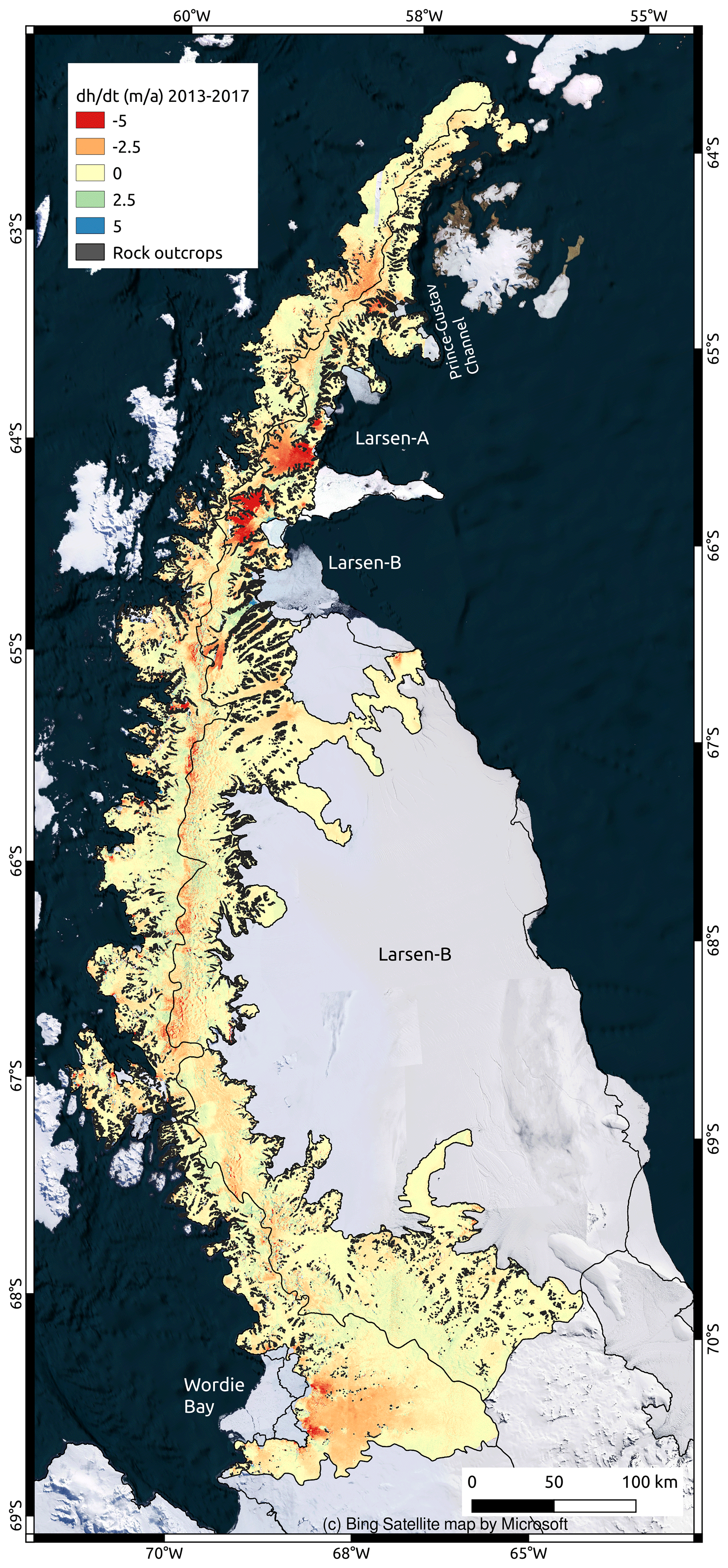
Figure 1Surface elevation changes between the austral winter of 2013 and 2017 were derived from TanDEM-X acquisitions for the 25g and 26g basins according to Zwally et al. (2012). Background: © Microsoft. Black polygons: rock outcrops according to Silva et al. (2020).
The study area is limited to the AP Ice Sheet north of 70∘ S, excluding the surrounding islands (see Fig. 1). This spatial extend was selected due to (1) the fact that this section of the AP is strongly affected by the disintegration of ice shelves; (2) the upwelling of CDW along the west coast; and (3) the limitations of mass budget estimates based on altimetry, gravimetry, and input–output method (see above). An area-wide geodetic mass balance assessment based on TanDEM-X data will provide an unprecedented spatially detailed and precise analysis and will be highly spatially complementary to the results based on other approaches for the more southern sections of the AP.
To obtain surface elevation information at the study site, bistatic synthetic aperture radar (SAR) acquisitions from the TanDEM-X mission were used. Several, mostly partial, TanDEM-X data coverages of the AP have existed since 2011. The surface conditions affect the SAR signal penetration depth in snow and ice (Abdullahi et al., 2018; Rott et al., 2021). A seasonal variability of the mean glacier surface height of about 2 m was reported for the northeastern AP using TDX data (Seehaus et al., 2015, 2016). However, according to Rott et al. (2018), differences in the SAR signal penetration of TDX can be neglected on the AP when comparing data from winter seasons. This assumption is based on comparing elevation changes from repeated TanDEM-X acquisitions and repeated airborne lidar measurements from NASA's Operation IceBridge. Consequently, we used two coverages of the AP with TDX data acquisitions from the austral winters of 2013 and 2017 for our analysis. A list of all individual TDX acquisitions and certain InSAR parameters can be found in the Supplement. A small data gap in the coverage from 2013 (9.6 %) was filled by TDX data from the austral winter of 2014 (see Fig. 2).
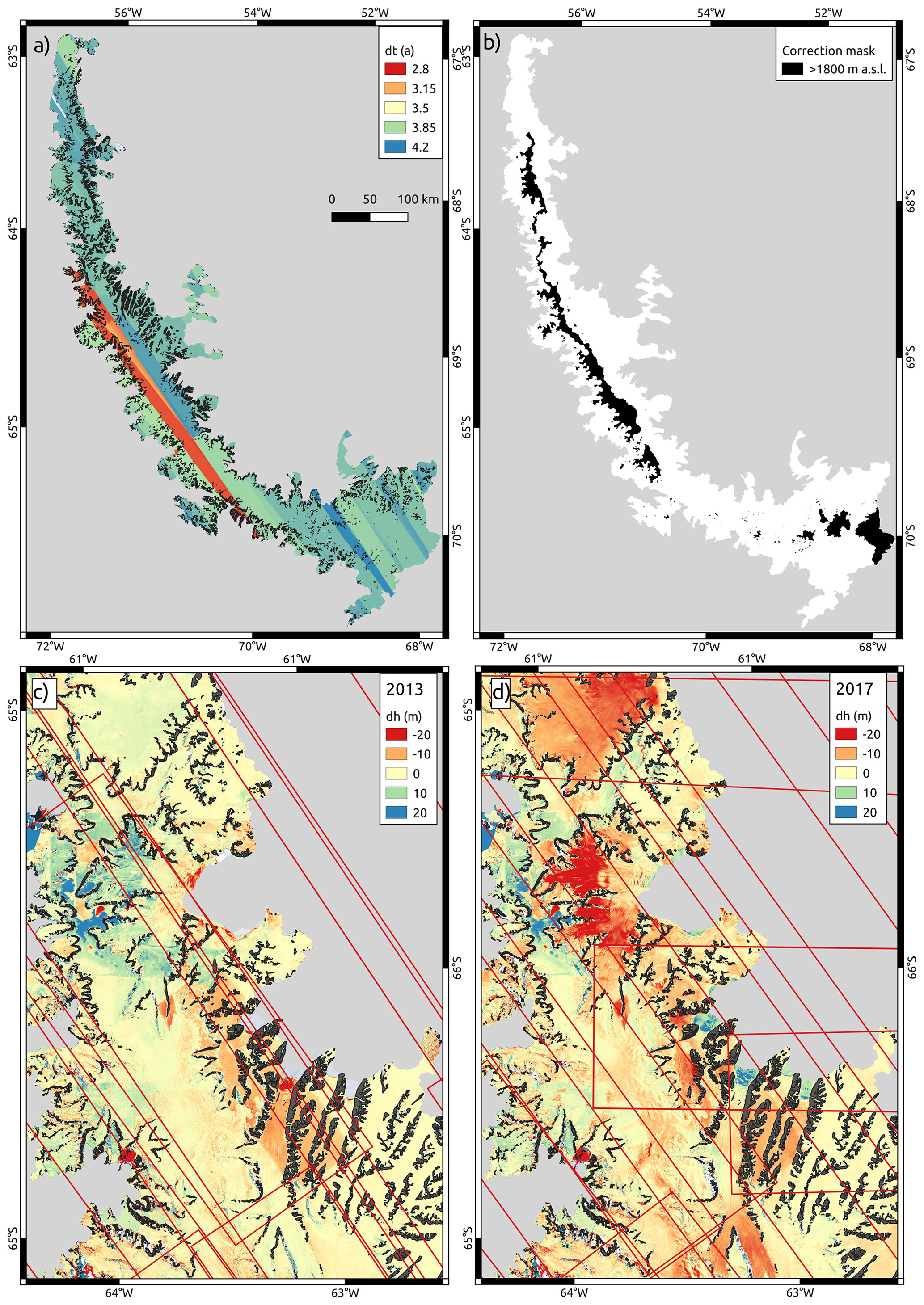
Figure 2(a) Time difference between elevation measurements. (b) Mask of areas above 1800 m a.s.l. used for radar penetration bias correction. (c) Election difference between refDEM and DEMs obtained in this study for 2013 and (d) for 2017. Black polygons: rock outcrops according to Silva et al. (2020).
A reference DEM (refDEM) is needed for the generation of SAR DEMs based on differential interferometry. The recently published high-resolution DEM of the AP (Dong et al., 2021) based on the global TanDEM-X DEM at 12 m spatial resolution is employed. The authors used information from the Reference Elevation Model of Antarctica (REMA) (Howat et al., 2019) to correct residual systematic elevation errors in the global TanDEM-X DEM and to obtain enhanced surface height data for the AP. The temporal coverage of the data used to generate the refDEM is comparable to our TDX coverage in 2013. However, no pixel-specific date information is available for the global TanDEM-X DEM and consequently for the refDEM, justifying the need to reprocess a surface elevation model for this time step.
Output from the regional climate model MAR (Modèle Atmosphérique Régional) covering the whole of Antarctica is used to obtain information on the CMB. MAR is a polar-oriented climate model mostly used to study the Greenland (Delhasse et al., 2020; Fettweis et al., 2021) and Antarctic ice sheets (Amory et al., 2021; Gilbert and Kittel, 2021). Hydrostatic approximation of primitive equations described in Gallée and Schayes (1994) is the basis of the atmosphere dynamics of the model, and its radiative transfer scheme is adapted from Morcrette (2002). The energy and mass transfer between the atmosphere and soil is handled by the SISVAT module (Soil Ice Snow Vegetation Atmospheric Transfer (De Ridder and Gallée, 1998)). For this study, the version used is MARv3.12, for which improvements have been described in Lambin et al. (2022). MAR was run over the AP at a 7.5 km spatial resolution and has been set to resolve the first 20 m of the snowpack, divided into 30 layers of varying thickness. The model is forced by the 6-hourly ERA-5 reanalysis (Hersbach et al., 2020) at the lateral boundaries and over the ocean between March 2006 and May 2022, but the data up to 2008 have been discarded as spin-up. The snowpack is initialized from a previous simulation (Kittel et al., 2021). The parameterization and evaluation of the model over the AP are described in Dethinne et al. (2023).
The average CMB is computed for the period July 2013 until June 2017, and the absolute and relative differences (dCMB) with respect to the whole temporal coverage of the MAR data (2008–2022) are computed to obtain information on CMB anomalies during the study period.
By dividing the CMB anomalies (dCMB) by the total mass change (), we define the mass balance ratio MBR. It indicates the contribution of CMB changes to the mass change. Positive values indicate that dCMB and are aligned, e.g., decreased CMB and total mass loss, whereas negative values point out contrary alignment, e.g., increased CMB and total mass loss. MBR values close to 1 indicate that the total mass changes can be mainly attributed to changes in CMB.
Information on individual glacier outlines, rock outcrops, and regional drainage basin definitions are taken from Silva et al. (2020), Rignot et al. (2011), and Zwally et al. (2012).
The TDX data were ordered in coregistered single-look complex (CoSSC) format. Consecutive acquisitions from the same date and orbit were concatenated to enhance the subsequent SAR processing and coregistration of the products. The differential interferometric SAR processing approach was applied to derive DEMs from the TDX data by means of the refDEM.
First, a differential interferogram is generated using the refDEM as an elevation reference. Afterward, the interferogram is filtered and unwrapped by applying the minimum-cost flow algorithm. The phase-to-height sensitivity is computed employing a simulated differential interferogram derived from the refDEM and the refDEM lowered by 100 m. Subsequently, the unwrapped differential interferogram based on the TDX data is converted to a differential elevation map by applying the derived phase-to-height sensitivity information. Finally, the height information of the refDEM is added to compute absolute heights, and the resulting DEM is orthorectified and geocoded. The advantage of this differential interferometric approach is that only the elevation difference between the refDEM and the TDX data needs to be unwrapped, leading to fewer phase-unwrapping issues in areas with complex topography like the AP.
The resulting TDX raw DEMs need to be coregistered to remove residual horizontal and vertical offsets, to generate a smooth DEM mosaic for each time step, and to facilitate the comparison of the DEMs from different dates. The iterative coregistration procedure consists of phase ramp removal operations and 3D coregistration based on the algorithm of Nuth and Kääb (2011). More details on the SAR processing and the coregistration procedure can be found in Sommer et al. (2022).
In previous studies (e.g., Braun et al., 2019; Malz et al., 2018; Sommer et al., 2022), the applied coregistration procedure was primarily based on the offset estimation between the refDEM and the TDX DEM on stable areas (ice-free land surfaces). At the AP, the number of ice-free areas is very limited. Less than 4 % of the surveyed area is not covered by glacier ice according to the rock masks from Silva et al. (2020). Moreover, many of the ice-free areas are situated on steep slopes, where DEMs are typically less reliable (Toutin, 2002) or where SAR layover and shadow limit the availability of elevation data in the individual raw TDX DEMs. Since the refDEM was generated based on TDX acquisitions in the austral winters of 2013 and 2014, it is assumed that the elevation differences between the refDEM and our TDX DEMs in 2013 and 2014 are minimal in most ice-covered areas. In particular, away from the dynamic glacier tongues and low-lying areas, previous studies reported only minor elevation change rates (Scambos et al., 2014; Seehaus et al., 2016). Consequently, the lower sections (<300 m a.s.l.) and dynamic glacier sections, manually defined utilizing NASA MEaSUREs ice velocity mosaics (Mouginot et al., 2017), were masked, out and the remaining ice-covered areas were included in the coregistration of TDX DEMs from 2013. The difference between the coregistered TDX DEMs and refDEM revealed some areas with remaining systematic elevation differences, e.g., caused by phase-unwrapping issues, in areas selected for coregistration. Those areas were manually inspected and masked out through an iterative process. For the TDX DEMs in 2017, an iterative procedure of coregistration relative to the refDEM was applied, consisting of DEMs differentiating and updating the masks. At later processing steps, potential biases caused by SAR signal penetration difference were observed at highly elevated areas (see below); consequently, these areas were also excluded in the iterative coregistration process. While doing this iterative masking, systematic elevation offsets were present in the elevation differences between the refDEM and both TDX DEM mosaics in some areas, mainly around the Larsen B embayment (see Fig. 2c and d). The offsets showed some patterns that can be attributed to the mosaicking of individual DEM tiles. The pattern does not fit the outlines of the individual DEMs used to generate the TDX DEM mosaics in this study. Thus, it is concluded that the remaining residual systematic elevation biases in the refDEM caused these offsets. Consequently, the affected areas were masked out during the coregistration process.
The resulting coregistered TDX DEM were mosaicked for both time steps and subtracted to obtain elevation change (dh) information. Mosaics consisting of pixel-wise date information were also generated to allow for a precise definition of elevation change rates (). Subsequently, the ice mass change rates () were computed using the Antarctic Ice Sheet basin definitions of 25g and 26g from Zwally et al. (2012) and I-Ipp from Rignot et al. (2011). Additionally, the basin delineations were cropped in latitudinal subsets in 1∘ steps to investigate potential spatial variations. The ice mass changes were also computed for individual glacier basins larger than 20 km2 using the most recent glacier outlines in the glacier inventory of Silva et al. (2020) and other local subregion definitions for comparison with existing studies (Rott et al., 2018; Scambos et al., 2014). Voids in the elevation change field on glacier areas were filled using local hypsometric interpolation for the analysis of the individual glaciers throughout the AP, which is one of the most suitable methods according to Seehaus et al. (2020b). The global hypsometric interpolation was applied for the analysis at basin and subregion scales. For all ice volume computations, the rock outcrop definition from Silva et al. (2020) was applied to mask out ice-free areas in the different ice sheet basin definitions. The ice volume changes were converted to mass changes using a volume-to-mass conversion factor of 900 kg m2. Since the most dominant ice volume changes are found for the various former ice shelf tributaries (see Fig. 1), this scenario is a suitable factor for ice mass changes dominated by ice dynamics (Kääb et al., 2012). The quality of the generated DEMs and elevation change data was evaluated using data from Operation IceBridge and time-stamped REMA (Reference Elevation Model of Antarctica) DEMs. A good agreement between the TanDEM-X data and the independent height information was obtained (TanDEM-X to Operation IceBridge: mean offset of 0.12 m a−1, RMSD of 0.34 m a−1; TanDEM-X to REMA for 2013 and 2017: mean offset −0.47 m a−1 and RMSD of 3.11 m a−1), which is an indication of the suitability of the TanDEM-X data for geodetic glacier mass balance assessments. A detailed description of the analysis and findings can be found in the Supplement.
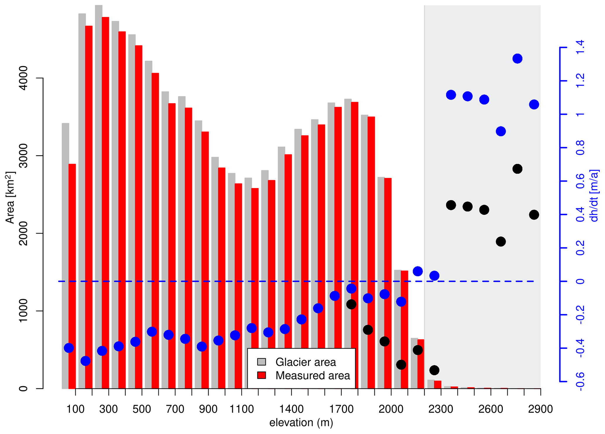
Figure 3Hypsometric distribution of measured (red bars) and total (gray bars) glacier area of 25g and 26g basins. Blue dots represent the mean value in each elevation interval, including corrections in areas above 1800 m a.s.l. Black dots indicate the uncorrected values. The gray area marks the upper 1 % quantile of the total glacier area distribution. Note that the scattered values in areas above 2300 m a.s.l. are located around one peak towards the southern border of the study area, where the steep slopes most likely lead to some biases. The affected area corresponds to only 0.06 % of the total glacier area, and thus its impact on the total mass budget can be neglected.
Based on a comparison with lidar measurements and on similarities in the backscatter coefficients, Rott et al. (2018) concluded that differences in the SAR signal penetration can be neglected when comparing TDX DEMs from austral winters on the AP. Even though solely TDX austral winter data are used in this analysis, some elevation change patterns in upper-glacier regions (see Fig. 1 and break in slope of the elevation change data in Fig. 3) seem to be caused by differences in the SAR signal penetration between the acquisitions. The analysis of the SAR backscatter coefficients and comparison with REMA DEM tiles also support this assumption (see Supplement). These areas are located at elevations above 1800 m a.s.l., covering an area of 12 306 km2 and corresponding to 16.4 % of the 25g and 26g drainage basins. In order to correct for these potential offsets, we applied a simple correction approach assuming a linearly increasing penetration correction of dh for the elevation range from 1800–2400 m a.s.l. of up to 2 m, similarly to Braun et al. (2019) or Seehaus et al. (2020a), leading to correction of the volume change of −2.76 km3 and an average elevation change of 0.04 m a−1 (25g and 26g basins). The upper limit of 2400 m a.s.l. was defined since only two small peaks in the southern part of the study area stretch above this limit. We are comparing X-band to X-band SAR data, in contrast to Braun et al. (2019), who compared X-band to C-band SAR data and applied a variable correction value of up to 5 m. Thus, a reduced maximum correction value of 2 m was selected based on the findings by Seehaus et al. (2015).
Finally, the ice mass change rate is computed with the following:
where S is the analyzed glacier area, Vpen is the volume change correction to account for differences in SAR signal penetration at higher elevations (see above), and ρ is the volume-to-mass conversion factor. The uncertainty of ice mass changes is computed with the following:
where is the uncertainty of the elevation change measurements, and δS is the uncertainty of the glacier outlines. Even though the ice loss is dominated by ice discharge, we account for uncertainties in the volume-to-mass conversion factor due to surface processes by applying a δρ of 60 kg m−3, as per Huss (2013).
To account adequately for the SAR signal penetration bias correction in the error budget of the mass changes, a 100 % uncertainty of Vpen is assumed. Vint is the uncertainty caused by the interpolation of in areas without measurements. It is computed by multiplying the glacier area with interpolated values by the uncertainty of caused by the interpolation (0.09 and 0.14 m a−1 for local and global hypsometric interpolation, respectively), which is computed according to Seehaus et al. (2020b).
was estimated based on slope-weighted elevation differences at ice-free areas and considering spatial auto-correlation according to Rolstad et al. (2009) using a correlation length of 318 m (Sommer et al., 2022). In order to account for potential local differences in the accuracy of the elevation changes, only ice-free areas within the individual ice sheet drainage basin, including the latitudinal subsets, were considered for the analysis of the different basins. Most individual glacier basins have very limited ice-free areas. Thus, the slope-weighted elevation differences revealed in the study-area-wide ice-free surfaces were used for the analysis at glacier scales. However, the individual glacier or basin area was used to account for spatial autocorrelation.
Since the ice sheet basin definitions from Zwally et al. (2012) and Rignot et al. (2011) are fixed standard products for mass balance computations in Antarctica, dS was set to zero when using these basin delineations. However, for the analysis of the individual glaciers, dS was estimated using the length of the ice–ocean glacier boundaries times a horizontal uncertainty ±60 m (reliability rating of 1 according to Ferrigno et al., 2006).
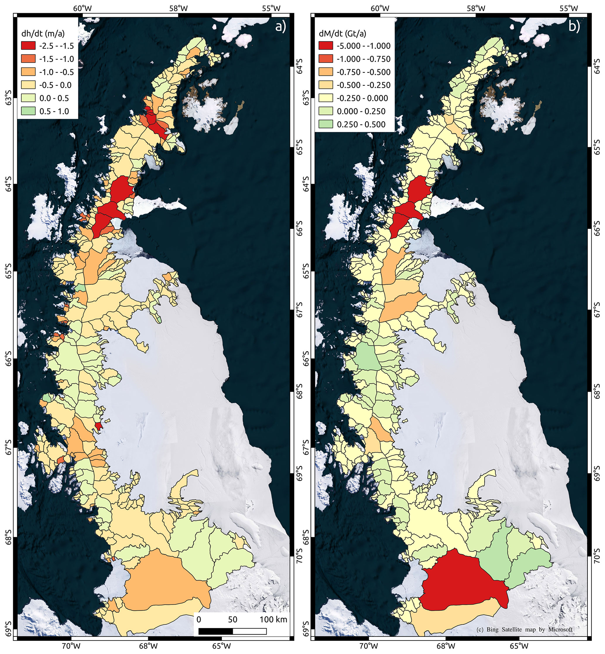
Figure 4(a) Average surface elevation changes () and (b) total mass changes () for individual glaciers >20 km2. Background: © Microsoft.
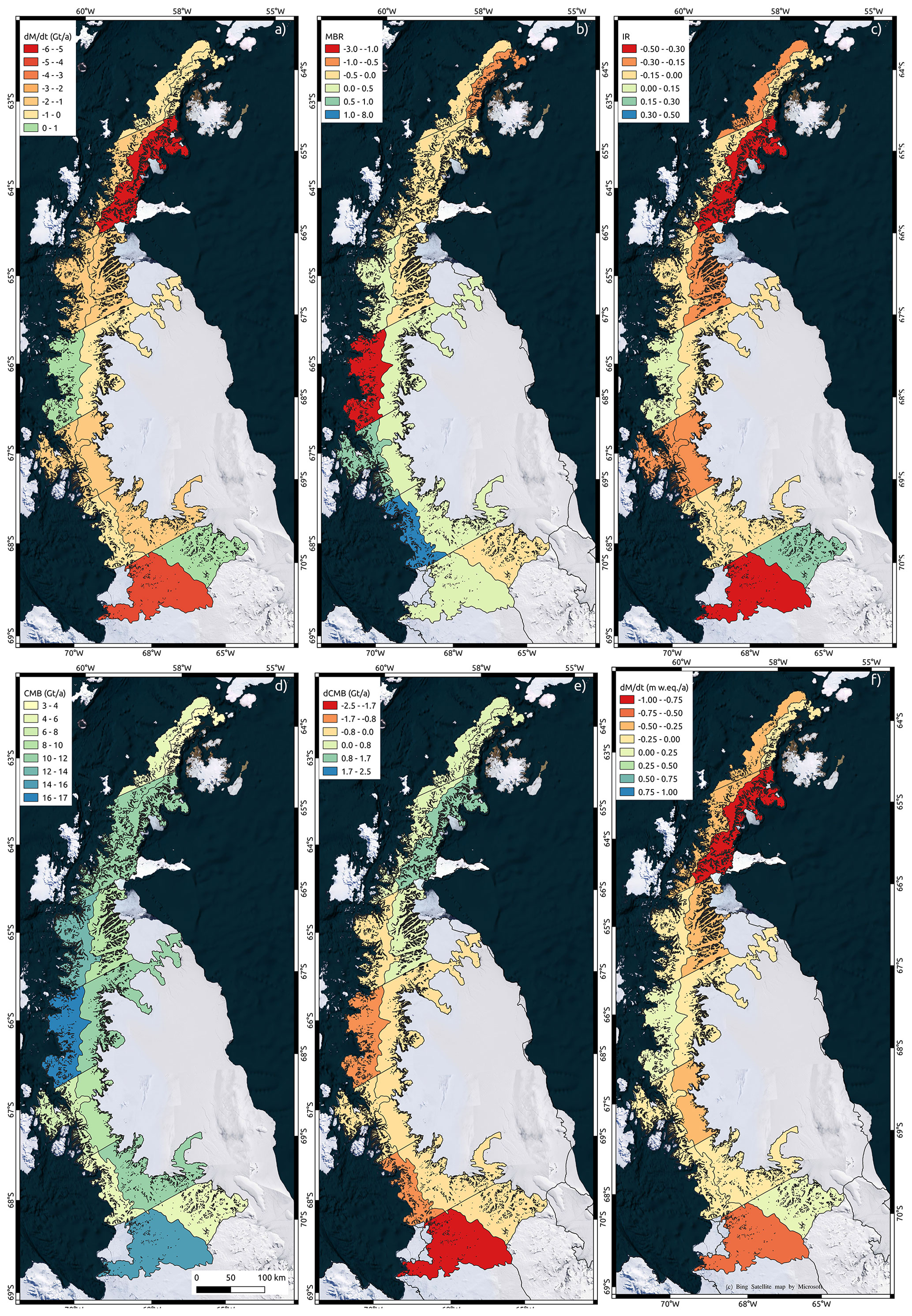
Figure 5(a) Total mass balance, (b) mass balance ratio, (c) imbalance ratio, (d) total climatic mass balance, (e) total climatic mass balance anomalies, and (f) specific mass balance for latitudinal subsets of the 25g and 26g drainage basins. Background: © Microsoft. Black polygons: rock outcrops according to Silva et al. (2020).
Table 1Summary of analyzed glacier area (S), glacier area covered by measurements (Sm), average surface lowering rate () (note that the listed uncertainty of represents the slope-weighted average offsets on rock outcrops, including consideration of spatial auto-correlation but not SAR signal penetration correction), total mass budget (), average climatic mass balance (CMB), imbalance ratio (IR), and mass balance ratio (MBR) for different basin and subregion definitions.
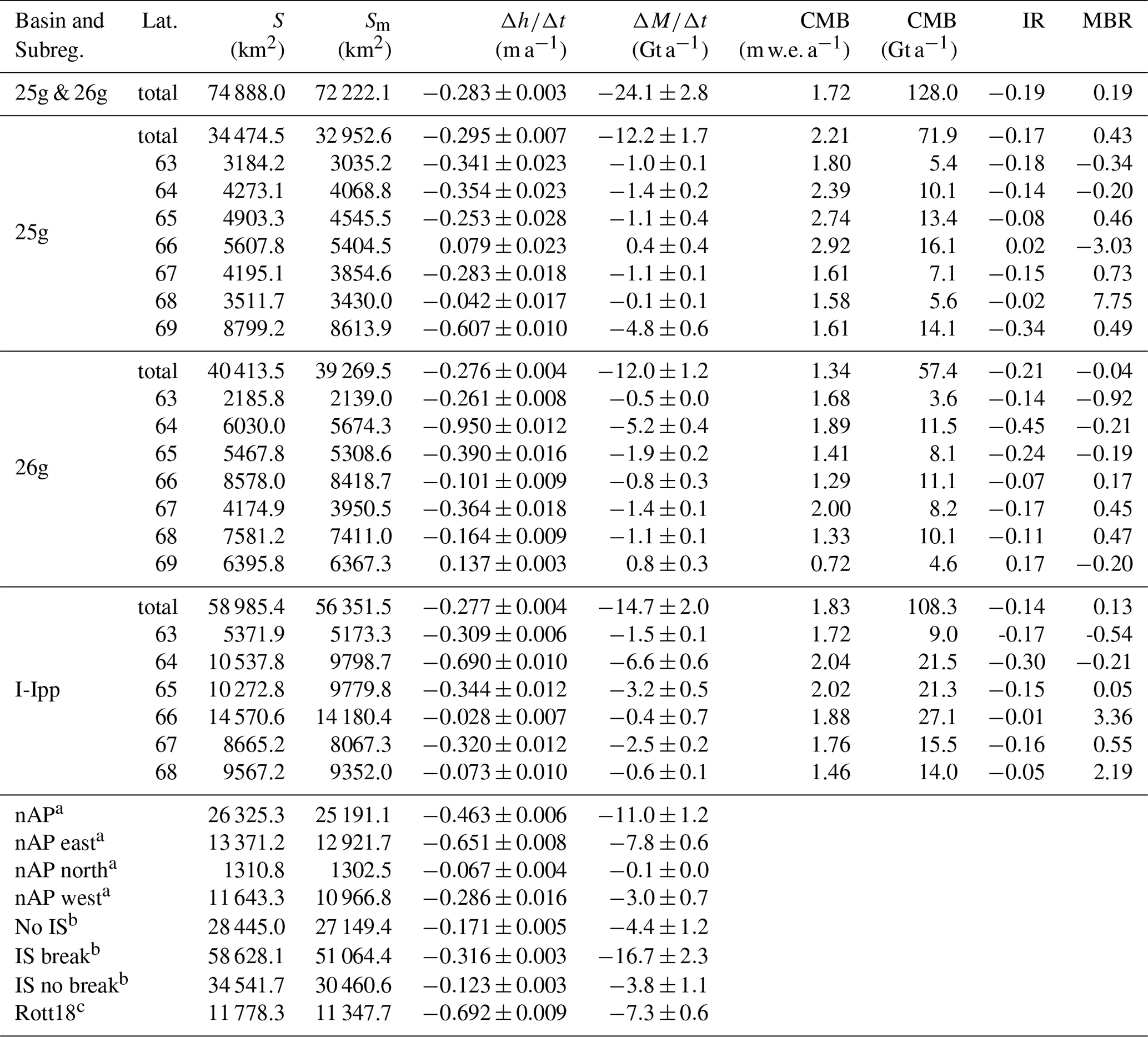
a Subregion definitions according to Scambos et al. (2014). b Subregion definitions based on glacier front type – No IS: non-ice shelf tributaries, IS break: former ice shelf tributaries, IS no break: current ice shelf tributaries. c Subregion definition according to Rott et al. (2018).
The revealed surface elevation information covers 96.4 % of the glaciated area of the northern AP Ice Sheet (basin definition 25g and 26g) and is illustrated in Fig. 1. The spatial distribution of the ice surface elevation changes indicates local hotspots of ice mass losses for some former ice shelf tributaries of the Larsen A and B and Wordie ice shelves. This spatial pattern also fits altimeter-based observations (Schröder et al., 2019; Shepherd et al., 2019). It is also clearly visible in the glacier-scale analysis of the ice mass changes, as illustrated in Fig. 4. Surface lowering rates of up to −8 m a−1 and more, as well as glacier-wide mean surface elevation change rates of , , and m a−1, are found for the Airy–Seller–Fleming (ASF), Drygalski, and Hektoria–Green–Evans (HGE) glaciers, respectively, which account for almost 40 % of the total mass loss of the study area. The overall highest value of Gt a−1 is found for ASF Glacier, which is the largest glacier (7710 km2) in the study area. The highest average surface lowering rate is observed at Drygalski Glacier. For a few, mainly small, glaciers, there are also slight positive mean values measured. Cook et al. (2016) proposed for the southwestern coast of the AP a correlation between frontal retreat and the warming of the mid-ocean water layer due to the upwelling of CDW since the 1990s. Walker and Gardner (2017), as well as Friedl et al. (2018), attributed the recession and increased ice discharge at Wordie Bay to the same phenomena. Our results confirm these propositions at Wordie Bay, where high ice losses are measured. However, further north, there is a very heterogeneous change pattern revealed on glacier scales (Fig. 4). By averaging the ice sheet changes on 1∘ latitudinal scales (Fig. 5 and Table 1), there is also no correlation observed with regard to the warming pattern reported by Cook et al. (2016). It is to be noted that the differences in the observation periods of this study and by Cook et al. (2016) (1945–2009) might explain the discrepancies. On the other hand, most glaciers along the west coast are situated in fjord-like valleys. Thus, the frontal retreat might not have destabilized the ice discharge. In order to test this hypothesis, further studies on the evolution of the ice flow are needed.
For section 66–67∘ S, an average slight mass gain is found, and for section 68–69∘ S, moderate ice loss is found. The comparison of with the average CMB and dCMB values (Fig. 5) on latitudinal scales does not show a correlation pattern. The dCMB indicates that the average CMB throughout the study period was lower in the southern and higher in the northern section of the study site in comparison to the long-term average CMB (Fig. 5e). The MBR values obtained in this study are illustrated in Fig. 5b and are listed in Table 1. Negative MBR is revealed for the northern part of the study area, indicating that changes in CMB were not the driver of mass losses. However, for wide parts of the Larsen C tributaries along the east coast and the southern section of the west coast, positive MBRs are revealed, suggesting that the decrease in CMB contributed to the total mass losses, particularly for the section between 67 and 69∘ S on the west coast. A negative MBR is revealed for section 66–67∘ S on the west coast. Here, a slight total mass gain and negative dCMB are found. Thus, it can be assumed that reduced ice discharge might have compensated for the lower CMB and may have even led to a mass gain. It is noteworthy that the modeled CMB is subject to considerable uncertainties, which can be assumed to be in the range of 14 %–17 % on the AP (Rignot et al., 2019), and that the revealed values have certain error margins as well. Thus, further analysis of the ice dynamics is needed to back up the drawn conclusions on correlations between CMB and , which is beyond the scope of this study.
The imbalance ratio, defined by Scambos et al. (2014) as the mass change divided by the CMB, serves as an indicator of the ice mass imbalance. It is illustrated in Fig. 5c and listed in Table 1. Its spatial pattern generally repeats the and MBR pattern and also clearly indicates the continuous high imbalance of the regions affected by the past ice shelf break-up events.
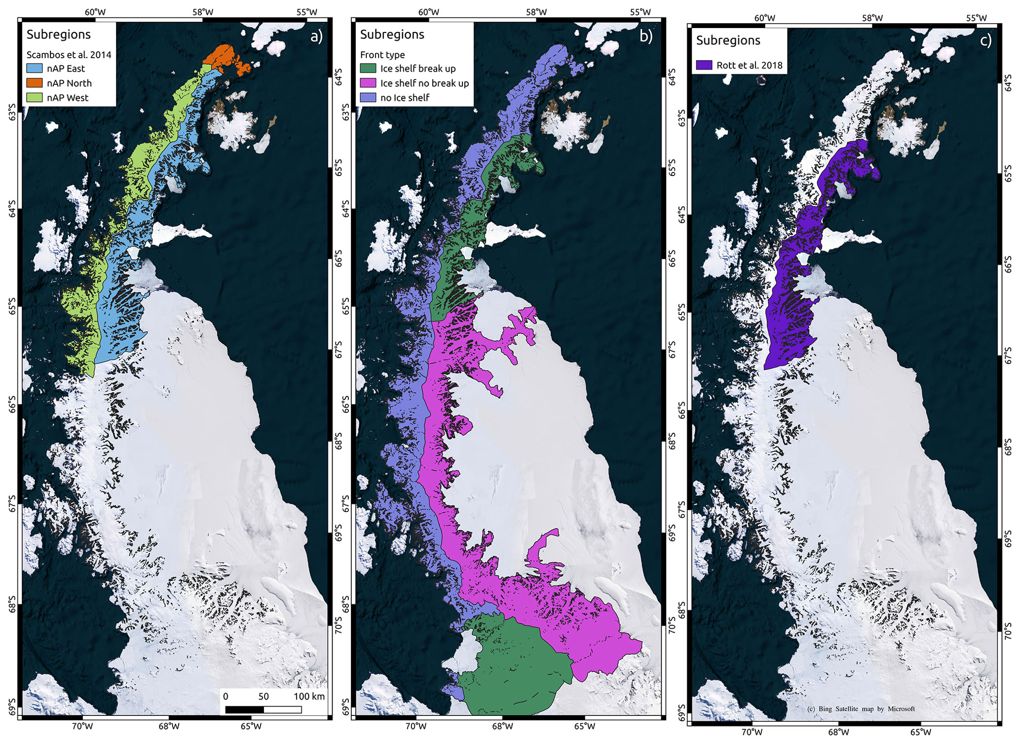
Figure 6Subregions of the total study site are based on (a) Scambos et al. (2014), (b) glacier front type, and (c) Rott et al. (2018). Background: © Microsoft. Black polygons: rock outcrops according to Silva et al. (2020).
By splitting the study side into subregions based on the glacier front type (see Fig. 6), average values of , , and m a−1 are found for former ice shelf tributaries, current ice shelf tributaries, and non-ice-shelf tributaries, respectively (Table 1). It indicates that the aftermath of the ice shelf break-up events forces increased mass losses of former tributaries even throughout multiple decades, accounting for 67 % of the study-area-wide mass loss.
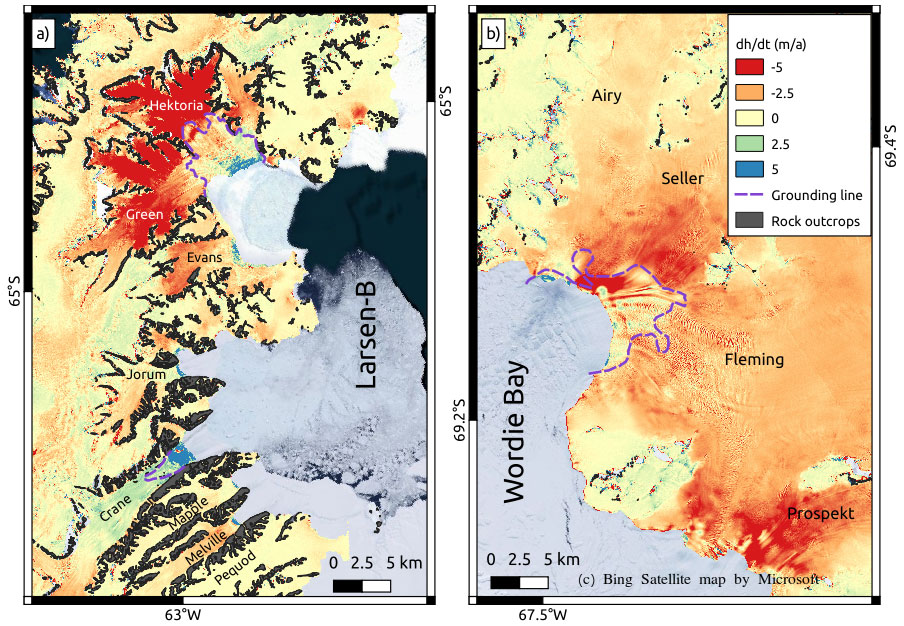
Figure 7(a) Grounding line positions at Hektoria–Green–Evans and Crane glaciers in 2016 from Rott et al. (2018) and (b) at Airy–Seller–Fleming Glacier in 2014 from Friedl et al. (2018) overlaid on the derived surface elevation changes between 2013 and 2017. Background: © Microsoft. Black polygons: rock outcrops according to Silva et al. (2020).
Along the coastline of the Larsen A and B and Wordie embayments, higher glacier flow speeds of the former ice shelf tributaries are reported by Rott et al. (2018), Seehaus et al. (2018), and Friedl et al. (2018) for the study period of this analysis. The observed ice thickness changes in this study are in accordance with the remaining accelerated ice discharge of these glaciers, which indicates imbalanced conditions. The most pronounced accelerated ice flows as compared to the pre-collapse conditions were reported for the Boydell, Sjögren, Drygalski, and Hektoria–Green glaciers. These observations fit well with the high ice thickness change rates in the range of −1.25 to −8.84 m a−1 found at these glaciers within this study and reported by Rott et al. (2018) for the period 2013–2016. Rott et al. (2018) observed a total mass budget for the analyzed glacier area (6358.7 km2, Fig. 6) of Gt a−1 (1.514±0.176 m a−1), which is comparable to our result (observed area: 11 685.6 km2) of Gt a−1 ( m a−1). The total mass budget agrees well. However, the average elevation change rates differ considerably, which can be explained by (1) slightly different observation periods; (2) different glacier outlines; (3) and, most importantly, the fact that Rott et al. (2018) analyzed only the lower, dynamic outlet glacier tongues (6358.7 km2 as compared to 12 723.4 km2 of the total area of all glaciers based on the outlines used by the authors). Based on this comparison, it can be concluded that the glacier tongues dominate the mass losses of the former tributaries due to the disintegration of the Larsen A and B ice shelves and that the higher-elevated plateau regions now show considerable changes, which is in accordance with Scambos et al. (2014) and our assumption for the coregistration process of the raw TDX DEMs. Moreover, the elevation change patterns on the Hektoria–Green Glacier revealed in this analysis support the assumption that wide parts of the lower glacier sections are floating. The distinct change from high surface lowering rates to much smaller rates towards the calving front indicates that the surface lowering signal by the thinning of the ice is widely compensated for by the buoyancy of the ice. A similar but less pronounced pattern is also visible at the Dinsmoor–Bombardier–Edgewoth (DBE) glacier system and was already discovered by Seehaus et al. (2015). The proposed grounding-line position based on our elevation change analysis is also comparable to the one suggested by Rott et al. (2020) for 2016 based on mapping a break in slope for Hektoria–Green Glacier (see Fig. 7). At Crane Glacier, Rott et al. (2020) also suggested a grounding-line position for 2016. However, our elevation change pattern does not allow a reasonable mapping of such a feature (note that the observed pronounced elevation increase towards the calving front is caused by frontal re-advance). At Wordie Bay (see Fig. 7), episodic glacier retreat and acceleration of Fleming Glacier were reported by Friedl et al. (2018), indicating its imbalance. Their suggested grounding-line position for 2014 fits partly to the elevation change pattern observed at the lower glacier sections in this study (see Fig. 7), similarly to the Hektoria-Green Glacier.
Scambos et al. (2014) carried out the spatially most extended (<66∘ S) geodetic analysis on the AP of glacier elevation and mass changes, primarily for the period 2003–2008. Due to the difference in the observation periods and the inclusion of the surrounding islands in the regional analysis, a direct comparison of their findings with ours is difficult, particularly due to dynamic changes of the former ice shelf tributaries along the east coast. However, the general spatial pattern is quite similar. They reported total mass loss rates of −24.9, −4.7, −2.3, and −18.0 Gt a−1 for the nAP <66∘ S, nAP west, nAP north, and nAP east (excluding the islands: −20.4, −3.9, −1.8, −14.8 Gt a−1; see Scambos et al. (2014) and Fig. 6 for region definitions), respectively, whereas we observed , , , and Gt a−1, respectively. Both analyses obtained similar moderate mass losses for the western sections. For the relatively small nAP north section, the difference might be caused by the very limited coverage of the area by DEM data in the study by Scambos et al. (2014). Elevated mass losses are found for the east coast by both analyses, which can be attributed to the imbalance of the former ice shelf tributaries in this section. Reduced mass losses are revealed for the more recent observation period by this study, which is in accordance with other analyses (e.g., Rott et al., 2018; Seehaus et al., 2018).
On drainage basin scales, a comparison with altimetry, gravimetric, and input–output-method-based estimates is feasible. Our revealed results for the different drainage basin definitions are summarized in Table 1. The gravimetric assessment of the mass budget of Antarctica by Groh and Horwath (2021) (https://data1.geo.tu-dresden.de/ais_gmb/, last access: 6 December 2022) suggests a mass balance for the AIS28 basin definition (corresponding to the 25g and 26g basins) of Gt a−1 for the period 16 June 2013 to 10 June 2017, whereas we observed Gt a−1. Even though both estimates agree within the error budget, there is a considerable difference in the nominal value. The huge uncertainty of the gravimetric-based estimate indicates the limitations of this approach for the study region. Moreover, the coarse spatial resolution does not allow for resolving detailed spatial patterns or even the analysis of the mass budget on glacier scales. The comparison with altimeter measurements is difficult since most analyses report results only on ice sheet basin scales and for much larger observation periods (e.g., Schröder et al., 2019; Shepherd et al., 2019). However, a meaningful comparison with Smith et al. (2020) is possible. The authors reported mass budgets of and Gt a−1 for the 25g and 26g basin definitions for the period 2003–2019, respectively. For basin 25g, the estimates agree well within the uncertainties with our findings. For basin 26g, they revealed higher mass loss rates. Their analysis starts in 2003, shortly after the disintegration of the Larsen B Ice Self and only a few years after the break-up of the Larsen A and Prince Gustav Channel ice shelves. Consequently, the dynamic ice mass loss of the former ice shelf tributaries located in basin 26g and the subsequent adjustments explain the difference compared to our estimate. Even though the uncertainties are much lower and the spatial resolution is higher than the altimeter-based estimates (e.g., 10 km for Schröder et al. (2019), 5 km for Shepherd et al. (2019)) compared to the gravimetric results, the revealed elevation change maps show a blurry pattern, hampering more spatially detailed analyses.
Table 2Comparison of glacier mass balances obtained in this study and by Rignot et al. (2019) for the period 2013–2017. S: glacier area. : total and specific mass balance.
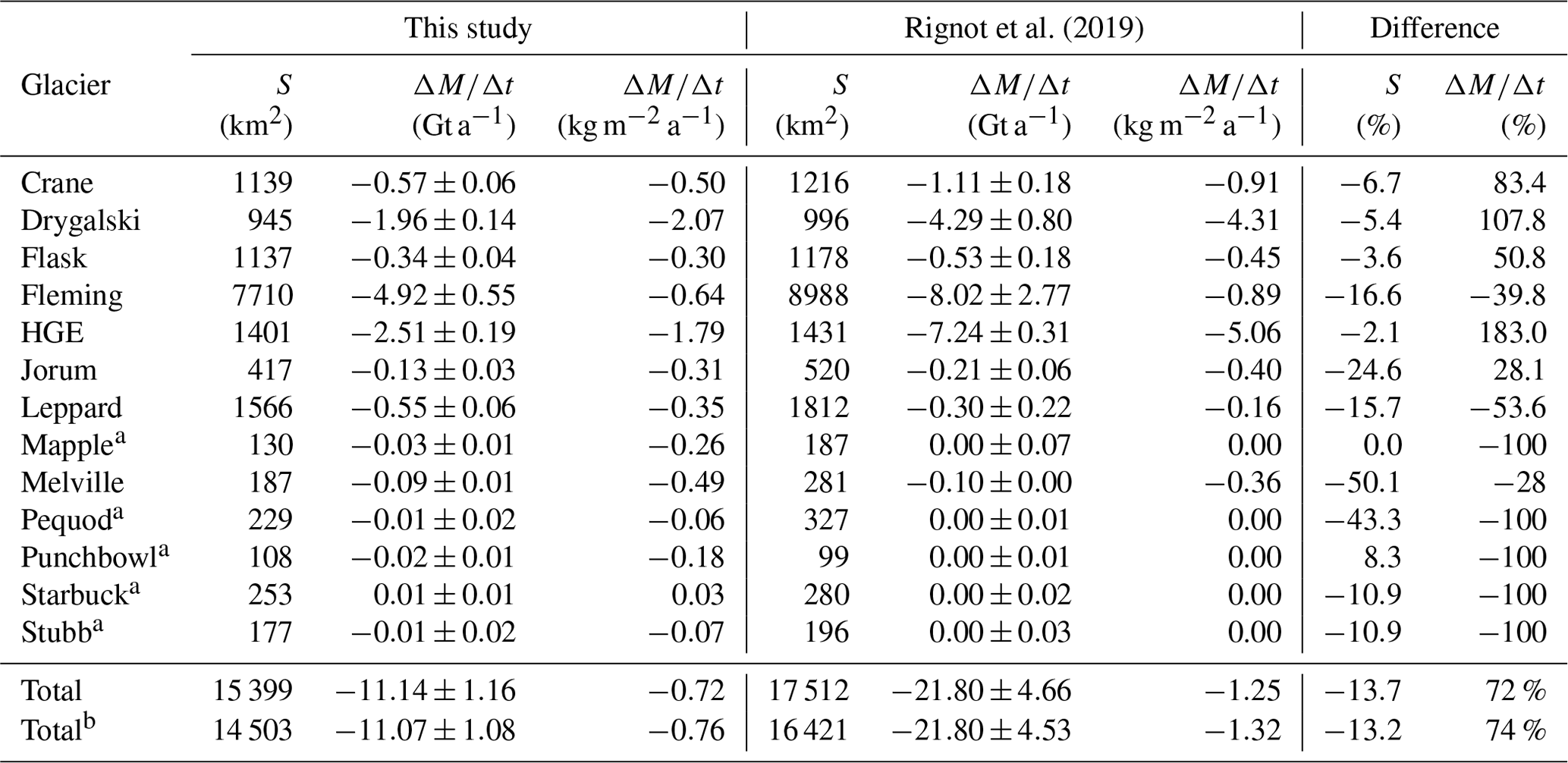
a Assumed balanced mass budget by Rignot et al. (2019). b Excluding glaciers with assumed balanced mass budget.
Rignot et al. (2019) provide mass balance estimates based on the input–output method on ice sheet basin scales but also for a few individual glaciers. Thus, a comparison on glacier scales is possible where the individual glaciers could be identified in the inventory used by them and by this study. Based on the supplementary information provided by Rignot et al. (2019), the mass budget was calculated by subtracting the average ice discharge in the years 2013–2017 from the reported reference SMB. A summary of the comparison with our results, mainly covering glaciers in the Larsen B embayment, is provided in Table 2. The considerable difference between our estimates of the total mass balance and the results by Rignot et al. (2019) can be partly attributed to differences in the glacier basin definitions. To compensate for the partially strong differences in the glacier basin areas, the specific mass balances were computed. However, for the specific mass balances, there are considerable deviations between both estimates as well even though our estimates agree well with the other geodetic estimates (see above). The limitations in reliable ice thickness estimates towards the grounding lines on the AP (see, e.g., Seehaus et al., 2015) and the applied assumptions to overcome these limitations by Rignot et al. (2019) are supposed to strongly bias the mass balance estimations. In particular, the balance conditions for some of the glaciers (Mapple, Pequod, Punchbowl, Starbuck, and Stubb Glacier) assumed by the authors need to be considered with care. For the SCAR-Inlet tributaries, namely Starbuck and Stubb, and for Pequod Glacier, it might be a suitable assumption; however, for the Mapple and Punchbowl glaciers, this assumption should be revised considering the specific mass balance estimates (see Table 2). On ice sheet basin scales, a mass budget of Gt a−1 for the I-Ipp basin is revealed by the input–output method, which overlaps with our estimate within the considerable error margins. It can be assumed that the result is most likely biased by the assumptions made to compensate for the missing good-quality ice thickness information in the study area.
By using repeated coverages of the northern AP by bi-static SAR data from austral winters in 2013 and 2017, it was possible to obtain a nearly full coverage (96.4 %) of ice surface elevation change measurements throughout the study area. The revealed spatial pattern of glacier changes and the overall mass budget of Gt a−1 agree well with other analyses. The detailed comparison of the revealed glacier changes at the Larsen A and B and Wordie embayments with other published data, based on elevation change measurements, highlights the suitability of the applied approach and the quality of the obtained results. However, the comparison with estimates based on the input–output method revealed strong deviations, particularly on glacier scales. These findings stress the need for improved ice thickness data towards the grounding line along the AP, which is the dominating error source in ice discharge estimates on the AP.
By including information on climatic mass balance, it could be identified that the observed mass changes can be, at least partly, attributed to climatic mass balance variations for wide parts of the southern section of the study area. However, most of the revealed mass losses are caused by ice dynamic changes. In particular, the still-ongoing increased ice discharge at the former ice shelf tributaries at the Prince Gustav Channel, Larsen A and B, and Wordie ice shelves are the hotspots of mass loss, and 67 % of the total mass loss throughout the study area can be attributed to these regions.
The previously reported correlation between increased frontal recession and mid-ocean warming along the southwestern coast of the study area could not be repeated by the surface elevation or mass change pattern observed in this analysis, excluding in Wordie Bay. It is probable that the ice flow of the well-confined glacier tongues in the fjord-like valleys did not get destabilized by the frontal retreat. To back-up this assumption and to further analyze the obtained glacier changes and their driving factors, a detailed analysis of the evolution of the ice dynamics throughout the study area would be desirable; this is, however, beyond the scope of this analysis.
This study provides the first geodetic assessment of glacier mass balances based on DEM differentiation throughout the northern AP at unprecedented spatially detailed scales and with high precision. The findings allow for ice elevation change and mass budget estimates on ice sheet basin and individual glacier scales, which will be beneficial for glaciological modeling, like enhanced ice thickness reconstructions, and for continental and global estimates of ice mass changes and sea level rise computations.
The code for the MAR data used in this study is tagged as v3.12 on https://gitlab.com/Mar-Group (MAR Team, 2022). Instructions to download the MAR code are provided at https://www.mar.cnrs.fr (last access: 10 November 2022).
Elevation change fields are available via the World Data Center PANGAEA, operated by AWI Bremerhaven (DOI is requested). The MAR outputs used in this study are available upon request by email (tdethinne@uliege.be).
The supplement related to this article is available online at: https://doi.org/10.5194/tc-17-4629-2023-supplement.
TS initiated, designed, and led the study, processed and analyzed the data, and wrote the paper. TS, PM, and CS developed jointly the analysis routines for elevation change and mass balance computations. TD contributed the MAR data and CMB analysis. All the authors revised the paper.
The contact author has declared that none of the authors has any competing interests.
Publisher's note: Copernicus Publications remains neutral with regard to jurisdictional claims made in the text, published maps, institutional affiliations, or any other geographical representation in this paper. While Copernicus Publications makes every effort to include appropriate place names, the final responsibility lies with the authors.
The authors would like to thank the German Aerospace Center for providing TanDEM-X data free of charge under AO XTI_GLAC0264. Aline Barbosa Silva kindly provided the glacier inventory of the AP from Silva et al. (2020). Peter Friedl kindly provided the groundling line data from Friedl et al. (2018). The TanDEM-X DEM of the AP used as a reference was kindly provided by Dana Floricioiu. ERA-5 reanalysis data (Hersbach et al., 2020) were provided by the European Centre for Medium-Range Weather Forecasts from their website at https://www.ecmwf.int/en/forecasts/datasets/reanalysis-datasets/era5 (last access: 24 October 2022). Computer resources were provided by Consortium des Équipements de Calcul Intensif (CÉCI), funded by the Fonds de la Recherche Scientifique de Belgique (F.R.S. – FNRS) under grant no. 2.5020.11, and by the Tier-1 supercomputer (Nic5) of the Fédération Wallonie Bruxelles infrastructure funded by the Walloon Region under grant agreement no. 1117545. Special thanks are given to Christoph Kittel for the help with the MAR data processing and evaluation. We acknowledge financial support by Deutsche Forschungsgemeinschaft and Friedrich-Alexander-Universität Erlangen-Nürnberg within the funding programme “Open Access Publication Funding”.
This research has been supported by the European Space Agency (Living Planet Fellowship MIT-AP), the Elitenetzwerk Bayern (grant no. IDP M3OCCA), and the Deutsche Forschungsgemeinschaft (grant no. DFG BR2105/14-2).
This paper was edited by Louise Sandberg Sørensen and reviewed by Aline Barbosa Silva and one anonymous referee.
Abdel Jaber, W., Rott, H., Floricioiu, D., Wuite, J., and Miranda, N.: Heterogeneous spatial and temporal pattern of surface elevation change and mass balance of the Patagonian ice fields between 2000 and 2016, The Cryosphere, 13, 2511–2535, https://doi.org/10.5194/tc-13-2511-2019, 2019.
Abdullahi, S., Wessel, B., Leichtle, T., Huber, M., Wohlfart, C., and Roth, A.: Investigation of Tandem-x Penetration Depth Over the Greenland Ice Sheet, in: IGARSS 2018–2018 IEEE International Geoscience and Remote Sensing Symposium, IGARSS 2018–2018 IEEE International Geoscience and Remote Sensing Symposium, 1336–1339, https://doi.org/10.1109/IGARSS.2018.8518930, 2018.
Amory, C., Kittel, C., Le Toumelin, L., Agosta, C., Delhasse, A., Favier, V., and Fettweis, X.: Performance of MAR (v3.11) in simulating the drifting-snow climate and surface mass balance of Adélie Land, East Antarctica, Geosci. Model Dev., 14, 3487–3510, https://doi.org/10.5194/gmd-14-3487-2021, 2021.
Braun, M. H., Malz, P., Sommer, C., Farías-Barahona, D., Sauter, T., Casassa, G., Soruco, A., Skvarca, P., and Seehaus, T. C.: Constraining glacier elevation and mass changes in South America, Nat. Clim. Change, 1, 130–136, https://doi.org/10.1038/s41558-018-0375-7, 2019.
Brun, F., Berthier, E., Wagnon, P., Kääb, A., and Treichler, D.: A spatially resolved estimate of High Mountain Asia glacier mass balances from 2000 to 2016, Nat. Geosci., 10, 668, https://doi.org/10.1038/ngeo2999, 2017.
Carrasco, J. F., Bozkurt, D., and Cordero, R. R.: A review of the observed air temperature in the Antarctic Peninsula. Did the warming trend come back after the early 21st hiatus?, Polar Sci., 28, 100653, https://doi.org/10.1016/j.polar.2021.100653, 2021.
Cook, A. J. and Vaughan, D. G.: Overview of areal changes of the ice shelves on the Antarctic Peninsula over the past 50 years, The Cryosphere, 4, 77–98, https://doi.org/10.5194/tc-4-77-2010, 2010.
Cook, A. J., Holland, P. R., Meredith, M. P., Murray, T., Luckman, A., and Vaughan, D. G.: Ocean forcing of glacier retreat in the western Antarctic Peninsula, Science, 353, 283–286, https://doi.org/10.1126/science.aae0017, 2016.
Delhasse, A., Kittel, C., Amory, C., Hofer, S., van As, D., S. Fausto, R., and Fettweis, X.: Brief communication: Evaluation of the near-surface climate in ERA5 over the Greenland Ice Sheet, The Cryosphere, 14, 957–965, https://doi.org/10.5194/tc-14-957-2020, 2020.
De Ridder, K. and Gallée, H.: Land Surface–Induced Regional Climate Change in Southern Israel, J. Appl. Meteorol., 37, 1470–1485, 1998.
Dethinne, T., Glaude, Q., Picard, G., Kittel, C., Alexander, P., Orban, A., and Fettweis, X.: Sensitivity of the MAR regional climate model snowpack to the parameterization of the assimilation of satellite-derived wet-snow masks on the Antarctic Peninsula, The Cryosphere, 17, 4267–4288, https://doi.org/10.5194/tc-17-4267-2023, 2023.
Dong, Y., Zhao, J., Floricioiu, D., Krieger, L., Fritz, T., and Eineder, M.: High-resolution topography of the Antarctic Peninsula combining the TanDEM-X DEM and Reference Elevation Model of Antarctica (REMA) mosaic, The Cryosphere, 15, 4421–4443, https://doi.org/10.5194/tc-15-4421-2021, 2021.
Dussaillant, I., Berthier, E., Brun, F., Masiokas, M., Hugonnet, R., Favier, V., Rabatel, A., Pitte, P., and Ruiz, L.: Two decades of glacier mass loss along the Andes, Nat. Geosci., 12, 1–7, https://doi.org/10.1038/s41561-019-0432-5, 2019.
Ferrigno, J. G., Cook, A. J., Foley, K. M., Williams, R. S., Swithinbank, C., Fox, A. J., Thomson, J. W., and Sievers, J.: Coastal-change and glaciological map of the Trinity Peninsula area and South Shetland Islands, Antarctica, 1843–2001, U.S. Dept. of the Interior, U.S. Geological Survey, Information Services, [Reston, Va.], Denver, Colo., 2006.
Fettweis, X., Hofer, S., Séférian, R., Amory, C., Delhasse, A., Doutreloup, S., Kittel, C., Lang, C., Van Bever, J., Veillon, F., and Irvine, P.: Brief communication: Reduction in the future Greenland ice sheet surface melt with the help of solar geoengineering, The Cryosphere, 15, 3013–3019, https://doi.org/10.5194/tc-15-3013-2021, 2021.
Friedl, P., Seehaus, T. C., Wendt, A., Braun, M. H., and Höppner, K.: Recent dynamic changes on Fleming Glacier after the disintegration of Wordie Ice Shelf, Antarctic Peninsula, The Cryosphere, 12, 1347–1365, https://doi.org/10.5194/tc-12-1347-2018, 2018.
Gallée, H. and Schayes, G.: Development of a Three-Dimensional Meso-γ Primitive Equation Model: Katabatic Winds Simulation in the Area of Terra Nova Bay, Antarctica, Mon. Weather Rev., 122, 671–685, https://doi.org/10.1175/1520-0493(1994)122<0671:DOATDM>2.0.CO;2, 1994.
Gilbert, E. and Kittel, C.: Surface Melt and Runoff on Antarctic Ice Shelves at 1.5 ∘C, 2 ∘C, and 4 ∘C of Future Warming, Geophys. Res. Lett., 48, e2020GL091733, https://doi.org/10.1029/2020GL091733, 2021.
Groh, A. and Horwath, M.: Antarctic Ice Mass Change Products from GRACE/GRACE-FO Using Tailored Sensitivity Kernels, Remote Sens., 13, 1736, https://doi.org/10.3390/rs13091736, 2021.
Hersbach, H., Bell, B., Berrisford, P., Hirahara, S., Horányi, A., Muñoz-Sabater, J., Nicolas, J., Peubey, C., Radu, R., Schepers, D., Simmons, A., Soci, C., Abdalla, S., Abellan, X., Balsamo, G., Bechtold, P., Biavati, G., Bidlot, J., Bonavita, M., De Chiara, G., Dahlgren, P., Dee, D., Diamantakis, M., Dragani, R., Flemming, J., Forbes, R., Fuentes, M., Geer, A., Haimberger, L., Healy, S., Hogan, R. J., Hólm, E., Janisková, M., Keeley, S., Laloyaux, P., Lopez, P., Lupu, C., Radnoti, G., de Rosnay, P., Rozum, I., Vamborg, F., Villaume, S., and Thépaut, J.-N.: The ERA5 global reanalysis, Q. J. Roy. Meteor. Soc., 146, 1999–2049, https://doi.org/10.1002/qj.3803, 2020.
Hogg, A. E. and Gudmundsson, G. H.: Impacts of the Larsen-C Ice Shelf calving event, Nat. Clim. Change, 7, 540–542, https://doi.org/10.1038/nclimate3359, 2017.
Hogg, A. E., Shepherd, A., Cornford, S. L., Briggs, K. H., Gourmelen, N., Graham, J. A., Joughin, I., Mouginot, J., Nagler, T., Payne, A. J., Rignot, E., and Wuite, J.: Increased ice flow in Western Palmer Land linked to ocean melting, Geophys. Res. Lett., 44, 2016GL072110, https://doi.org/10.1002/2016GL072110, 2017.
Holland, P. R., Jenkins, A., and Holland, D. M.: Ice and ocean processes in the Bellingshausen Sea, Antarctica, J. Geophys. Res., 115, C05020, https://doi.org/10.1029/2008JC005219, 2010.
Holland, P. R., Brisbourne, A., Corr, H. F. J., McGrath, D., Purdon, K., Paden, J., Fricker, H. A., Paolo, F. S., and Fleming, A. H.: Oceanic and atmospheric forcing of Larsen C Ice-Shelf thinning, The Cryosphere, 9, 1005–1024, https://doi.org/10.5194/tc-9-1005-2015, 2015.
Horwath, M. and Dietrich, R.: Signal and error in mass change inferences from GRACE: the case of Antarctica, Geophys. J. Int., 177, 849–864, https://doi.org/10.1111/j.1365-246X.2009.04139.x, 2009.
Howat, I. M., Porter, C., Smith, B. E., Noh, M.-J., and Morin, P.: The Reference Elevation Model of Antarctica, The Cryosphere, 13, 665–674, https://doi.org/10.5194/tc-13-665-2019, 2019.
Hugonnet, R., McNabb, R., Berthier, E., Menounos, B., Nuth, C., Girod, L., Farinotti, D., Huss, M., Dussaillant, I., Brun, F., and Kääb, A.: Accelerated global glacier mass loss in the early twenty-first century, Nature, 592, 726–731, https://doi.org/10.1038/s41586-021-03436-z, 2021.
Huss, M.: Density assumptions for converting geodetic glacier volume change to mass change, The Cryosphere, 7, 877–887, https://doi.org/10.5194/tc-7-877-2013, 2013.
IMBIE Team: Mass balance of the Antarctic Ice Sheet from 1992 to 2017, Nature, 558, 219, https://doi.org/10.1038/s41586-018-0179-y, 2018.
Kääb, A., Berthier, E., Nuth, C., Gardelle, J., and Arnaud, Y.: Contrasting patterns of early twenty-first-century glacier mass change in the Himalayas, Nature, 488, 495–498, https://doi.org/10.1038/nature11324, 2012.
Kittel, C., Amory, C., Agosta, C., Jourdain, N. C., Hofer, S., Delhasse, A., Doutreloup, S., Huot, P.-V., Lang, C., Fichefet, T., and Fettweis, X.: Diverging future surface mass balance between the Antarctic ice shelves and grounded ice sheet, The Cryosphere, 15, 1215–1236, https://doi.org/10.5194/tc-15-1215-2021, 2021.
Lambin, C., Fettweis, X., Kittel, C., Fonder, M., and Ernst, D.: Assessment of future wind speed and wind power changes over South Greenland using the Modèle Atmosphérique Régional regional climate model, Int. J. Climatol., 43, joc.7795, https://doi.org/10.1002/joc.7795, 2022.
Malz, P., Meier, W., Casassa, G., Jaña, R., Skvarca, P., and Braun, M. H.: Elevation and Mass Changes of the Southern Patagonia Icefield Derived from TanDEM-X and SRTM Data, Remote Sens., 10, 188, https://doi.org/10.3390/rs10020188, 2018.
MAR Team: MARv3.12, MAR Team [code], https://gitlab.com/Mar-Group/ (last access: 16 November 2022), 2022.
Morcrette, J.-J.: Assessment of the ECMWF Model Cloudiness and Surface Radiation Fields at the ARM SGP Site, Mon. Weather Rev., 130, 257–277, 2002.
Mouginot, J., Rignot, E., Scheuchl, B., and Millan, R.: Comprehensive Annual Ice Sheet Velocity Mapping Using Landsat-8, Sentinel-1, and RADARSAT-2 Data, Remote Sens., 9, 364, https://doi.org/10.3390/rs9040364, 2017.
Nuth, C. and Kääb, A.: Co-registration and bias corrections of satellite elevation data sets for quantifying glacier thickness change, The Cryosphere, 5, 271–290, https://doi.org/10.5194/tc-5-271-2011, 2011.
Oliva, M., Navarro, F., Hrbáček, F., Hernández, A., Nývlt, D., Pereira, P., Ruiz-Fernández, J., and Trigo, R.: Recent regional climate cooling on the Antarctic Peninsula and associated impacts on the cryosphere, Sci. Total Environ., 580, 210–223, https://doi.org/10.1016/j.scitotenv.2016.12.030, 2017.
Rignot, E., Mouginot, J., and Scheuchl, B.: Ice Flow of the Antarctic Ice Sheet, Science, 333, 1427–1430, https://doi.org/10.1126/science.1208336, 2011.
Rignot, E., Mouginot, J., Scheuchl, B., van den Broeke, M., van Wessem, M. J., and Morlighem, M.: Four decades of Antarctic Ice Sheet mass balance from 1979–2017, P. Natl. Acad. Sci. USA, 116, 201812883, https://doi.org/10.1073/pnas.1812883116, 2019.
Rolstad, C., Haug, T., and Denby, B.: Spatially integrated geodetic glacier mass balance and its uncertainty based on geostatistical analysis: application to the western Svartisen ice cap, Norway, J. Glaciol., 55, 666–680, https://doi.org/10.3189/002214309789470950, 2009.
Rott, H., Müller, F., Nagler, T., and Floricioiu, D.: The imbalance of glaciers after disintegration of Larsen-B ice shelf, Antarctic Peninsula, The Cryosphere, 5, 125–134, https://doi.org/10.5194/tc-5-125-2011, 2011.
Rott, H., Floricioiu, D., Wuite, J., Scheiblauer, S., Nagler, T., and Kern, M.: Mass changes of outlet glaciers along the Nordensjköld Coast, northern Antarctic Peninsula, based on TanDEM-X satellite measurements, Geophys. Res. Lett., 41, 2014GL061613, https://doi.org/10.1002/2014GL061613, 2014.
Rott, H., Abdel Jaber, W., Wuite, J., Scheiblauer, S., Floricioiu, D., van Wessem, J. M., Nagler, T., Miranda, N., and van den Broeke, M. R.: Changing pattern of ice flow and mass balance for glaciers discharging into the Larsen A and B embayments, Antarctic Peninsula, 2011 to 2016, The Cryosphere, 12, 1273–1291, https://doi.org/10.5194/tc-12-1273-2018, 2018.
Rott, H., Wuite, J., De Rydt, J., Gudmundsson, G. H., Floricioiu, D., and Rack, W.: Impact of marine processes on flow dynamics of northern Antarctic Peninsula outlet glaciers, Nat. Commun., 11, 2969, https://doi.org/10.1038/s41467-020-16658-y, 2020.
Rott, H., Scheiblauer, S., Wuite, J., Krieger, L., Floricioiu, D., Rizzoli, P., Libert, L., and Nagler, T.: Penetration of interferometric radar signals in Antarctic snow, The Cryosphere, 15, 4399–4419, https://doi.org/10.5194/tc-15-4399-2021, 2021.
Scambos, T., Hulbe, C., and Fahnestock, M.: Climate-Induced Ice Shelf Disintegration in the Antarctic Peninsula, in: Antarctic Peninsula Climate Variability: Historical and Paleoenvironmental Perspectives, edited by: Domack, E., Levente, A., Burnet, A., Bindschadler, R., Convey, P., and Kirby, M., American Geophysical Union, 79–92, 2003.
Scambos, T. A.: Glacier acceleration and thinning after ice shelf collapse in the Larsen B embayment, Antarctica, Geophys. Res. Lett., 31, L18402, https://doi.org/10.1029/2004GL020670, 2004.
Scambos, T. A., Berthier, E., Haran, T., Shuman, C. A., Cook, A. J., Ligtenberg, S. R. M., and Bohlander, J.: Detailed ice loss pattern in the northern Antarctic Peninsula: widespread decline driven by ice front retreats, The Cryosphere, 8, 2135–2145, https://doi.org/10.5194/tc-8-2135-2014, 2014.
Schröder, L., Horwath, M., Dietrich, R., Helm, V., van den Broeke, M. R., and Ligtenberg, S. R. M.: Four decades of Antarctic surface elevation changes from multi-mission satellite altimetry, The Cryosphere, 13, 427–449, https://doi.org/10.5194/tc-13-427-2019, 2019.
Seehaus, T., Marinsek, S., Helm, V., Skvarca, P., and Braun, M.: Changes in ice dynamics, elevation and mass discharge of Dinsmoor–Bombardier–Edgeworth glacier system, Antarctic Peninsula, Earth Planet. Sc. Lett., 427, 125–135, 2015.
Seehaus, T., Cook, A. J., Silva, A. B., and Braun, M.: Changes in glacier dynamics in the northern Antarctic Peninsula since 1985, The Cryosphere, 12, 577–594, https://doi.org/10.5194/tc-12-577-2018, 2018.
Seehaus, T., Malz, P., Sommer, C., Lippl, S., Cochachin, A., and Braun, M.: Changes of the tropical glaciers throughout Peru between 2000 and 2016 – mass balance and area fluctuations, The Cryosphere, 13, 2537–2556, https://doi.org/10.5194/tc-13-2537-2019, 2019.
Seehaus, T., Malz, P., Sommer, C., Soruco, A., Rabatel, A., and Braun, M.: Mass balance and area changes of glaciers in the Cordillera Real and Tres Cruces, Bolivia, between 2000 and 2016, J. Glaciol., 66, 124–136, https://doi.org/10.1017/jog.2019.94, 2020a.
Seehaus, T., Morgenshtern, V. I., Hübner, F., Bänsch, E., and Braun, M. H.: Novel Techniques for Void Filling in Glacier Elevation Change Data Sets, Remote Sens., 12, 3917, https://doi.org/10.3390/rs12233917, 2020b.
Seehaus, T. C., Marinsek, S., Skvarca, P., van Wessem, J. M., Reijmer, C. H., Seco, J. L., and Braun, M. H.: Dynamic Response of Sjögren Inlet Glaciers, Antarctic Peninsula, to Ice Shelf Breakup Derived from Multi-Mission Remote Sensing Time Series, Front. Earth Sci., 4, https://doi.org/10.3389/feart.2016.00066, 2016.
Shepherd, A., Gilbert, L., Muir, A. S., Konrad, H., McMillan, M., Slater, T., Briggs, K. H., Sundal, A. V., Hogg, A. E., and Engdahl, M. E.: Trends in Antarctic Ice Sheet Elevation and Mass, Geophys. Res. Lett., 46, 8174–8183, https://doi.org/10.1029/2019GL082182, 2019.
Silva, A. B., Arigony-Neto, J., Braun, M. H., Espinoza, J. M. A., Costi, J., and Janã, R.: Spatial and temporal analysis of changes in the glaciers of the Antarctic Peninsula, Global Planet. Change, 184, 103079, https://doi.org/10.1016/j.gloplacha.2019.103079, 2020.
Smith, B., Fricker, H. A., Gardner, A. S., Medley, B., Nilsson, J., Paolo, F. S., Holschuh, N., Adusumilli, S., Brunt, K., Csatho, B., Harbeck, K., Markus, T., Neumann, T., Siegfried, M. R., and Zwally, H. J.: Pervasive ice sheet mass loss reflects competing ocean and atmosphere processes, Science, 368, 1239–1242, https://doi.org/10.1126/science.aaz5845, 2020.
Sommer, C., Seehaus, T., Glazovsky, A., and Braun, M. H.: Brief communication: Increased glacier mass loss in the Russian High Arctic (2010–2017), The Cryosphere, 16, 35–42, https://doi.org/10.5194/tc-16-35-2022, 2022.
Toutin, T.: Three-dimensional topographic mapping with ASTER stereo data in rugged topography, IEEE T. Geosci. Remote, 40, 2241–2247, https://doi.org/10.1109/TGRS.2002.802878, 2002.
Turner, J., Lu, H., White, I., King, J. C., Phillips, T., Hosking, J. S., Bracegirdle, T. J., Marshall, G. J., Mulvaney, R., and Deb, P.: Absence of 21st century warming on Antarctic Peninsula consistent with natural variability, Nature, 535, 411–415, https://doi.org/10.1038/nature18645, 2016.
Vaughan, D. G., Marshall, G. J., Connolley, W. M., Parkinson, C., Mulvaney, R., Hodgson, D. A., King, J. C., Pudsey, C. J., and Turner, J.: Recent rapid regional climate warming on the Antarctic Peninsula, Clim. Change, 60, 243–274, 2003.
Walker, C. C. and Gardner, A. S.: Rapid drawdown of Antarctica's Wordie Ice Shelf glaciers in response to ENSO/Southern Annular Mode-driven warming in the Southern Ocean, Earth Planet. Sc. Lett., 476, 100–110, https://doi.org/10.1016/j.epsl.2017.08.005, 2017.
Wendt, J., Rivera, A., Wendt, A., Bown, F., Zamora, R., Casassa, G., and Bravo, C.: Recent ice-surface-elevation changes of Fleming Glacier in response to the removal of the Wordie Ice Shelf, Antarctic Peninsula, Ann. Glaciol., 51, 97–102, 2010.
Wouters, B., Martin-Español, A., Helm, V., Flament, T., van Wessem, J. M., Ligtenberg, S. R. M., van den Broeke, M. R., and Bamber, J. L.: Dynamic thinning of glaciers on the Southern Antarctic Peninsula, Science, 348, 899–903, https://doi.org/10.1126/science.aaa5727, 2015.
Wuite, J., Rott, H., Hetzenecker, M., Floricioiu, D., De Rydt, J., Gudmundsson, G. H., Nagler, T., and Kern, M.: Evolution of surface velocities and ice discharge of Larsen B outlet glaciers from 1995 to 2013, The Cryosphere, 9, 957–969, https://doi.org/10.5194/tc-9-957-2015, 2015.
Zwally, H. J., Giovinetto, M., Beckley, M. A., and Saba, J. L.: Antarctic and Greenland Drainage Systems, GSFC Cryospheric Sciences Laboratory, https://earth.gsfc.nasa.gov/cryo/data/polar-altimetry/antarctic-and-greenland-drainage-systems (last access: 2 November 2023), 2012.