the Creative Commons Attribution 4.0 License.
the Creative Commons Attribution 4.0 License.
 | 03 Feb 2023
Evolution of the dynamics, area, and ice production of the Amundsen Sea Polynya, Antarctica, 2016–2021
Grant J. Macdonald
Stephen F. Ackley
Alberto M. Mestas-Nuñez
Adrià Blanco-Cabanillas
Polynyas are key sites of ice production during the winter and are important sites of biological activity and carbon sequestration during the summer. The Amundsen Sea Polynya (ASP) is the fourth largest Antarctic polynya, has recorded the highest primary productivity, and lies in an embayment of key oceanographic significance. However, knowledge of its dynamics, and of sub-annual variations in its area and ice production, is limited. In this study we primarily utilize Sentinel-1 synthetic aperture radar (SAR) imagery, sea ice concentration products, and climate reanalysis data, along with bathymetric data, to analyze the ASP over the period November 2016–March 2021. Specifically, we analyze (i) qualitative changes in the ASP's characteristics and dynamics, as well as quantitative changes in (ii) summer polynya area, and (iii) winter polynya area and ice production. From our analysis of SAR imagery we find that ice produced by the ASP becomes stuck in the vicinity of the polynya and sometimes flows back into the polynya, contributing to its closure and limiting further ice production. The polynya forms westward off a persistent chain of grounded icebergs that are located at the site of a bathymetric high. Grounded icebergs also influence the outflow of ice and facilitate the formation of a “secondary polynya” at times. Additionally, unlike some polynyas, ice produced by the polynya flows westward after formation, along the coast and into the neighboring sea sector. During the summer and early winter, broader regional sea ice conditions can play an important role in the polynya. The polynya opens in all summers, but record-low sea ice conditions in 2016/17 cause it to become part of the open ocean. During the winter, an average of 78 % of ice production occurs in April–May and September–October, but large polynya events often associated with high, southeasterly or easterly winds can cause ice production throughout the winter. While passive microwave data or daily sea ice concentration products remain key for analyzing variations in polynya area and ice production, we find that the ability to directly observe and qualitatively analyze the polynya at a high temporal and spatial resolution with Sentinel-1 imagery provides important insights about the behavior of the polynya that are not possible with those datasets.
- Article
(18821 KB) - Full-text XML
-
Supplement
(5591 KB) - BibTeX
- EndNote


Coastal polynyas, or “latent heat polynyas” (henceforth referred to simply as “polynyas”), are sites of open water surrounded by sea ice and land, glacier ice, or fast ice (Armstrong, 1972; Tamura et al., 2008; Park et al., 2018). These polynyas are distributed around the coast of Antarctica and are typically at fixed geographic locations each year. They develop because the ice that forms at these sites is regularly driven away by winds or ocean currents, creating an opening in the sea ice (Bromwich and Kurtz, 1984; Bromwich et al., 1993, 1998; Morales Maqueda et al., 2004; Sansiviero et al., 2017).
Between the Antarctic summer months of approximately November and March, these open-water sites tend to remain persistently ice-free. Among other factors, the combination of ice-free conditions, summer sunlight, and the availability of dissolved iron (e.g., Arrigo et al., 2008a, 2012; St-Laurent et al., 2017) enables large phytoplankton blooms to develop in polynyas during this summer period. These phytoplankton blooms fix carbon from dissolved carbon dioxide, some of which then sinks below the surface layer (Sweeney et al., 2003). As a result, the evolution of polynyas during the summer is considered a key factor in the primary productivity of the Southern Ocean and, consequently, also their role in the sequestration of carbon dioxide (the “biological pump”) (Arrigo et al., 2008b).
Between the Antarctic winter months of approximately April and October polynyas tend to be intermittently active and are smaller in area than in the summer. When a polynya does open during the winter, excess ocean heat is lost and new sea ice production takes place approximately immediately in the opened area. Winds (usually katabatic winds) or ocean currents later push the newly produced sea ice away and open the polynya again, causing yet more ice to form. Repeated polynya events produce new sea ice throughout the winter period and hence polynyas have been termed “factories” of sea ice production (Kimura and Wakatsuchi, 2004; Assmann et al., 2005). Overall, polynyas are estimated to contribute around 10 % of all Antarctic sea ice cover (Tamura et al., 2008; Nihashi and Oshima, 2015). Regionally, polynyas can play an even larger role in production. For example, the Ross Ice Shelf Polynya is estimated to produce several cubic kilometers of ice annually, and along with the McMurdo Sound Polynya, it may produce 20 %–50 % of total sea ice in the region (Drucker et al., 2011). The polynya-produced ice then forms part of the pack ice, contributing to its characteristics and potentially further thickening it due to deformation. For example, ice formed by the Terra Nova Bay polynya in the western Ross Sea had a mean thickness 3–4 times that of the central Ross Sea, with 80 % of the ice contained in deformed ice and ridges (Rack et al., 2020). Consequently, understanding of polynya evolution through the winter is important for understanding ice production and sea ice characteristics in the Southern Ocean.
The Amundsen Sea Polynya (ASP), West Antarctica, and the embayment in which it lies are of particular interest for several reasons. The polynya is situated in the embayment into which the Thwaites and Pine Island glaciers terminate and undergo ocean-driven melting, making the oceanography of the embayment of special interest (IMBIE team, 2018; Rignot et al., 2019). The ASP is also known to be a key site of primary productivity in the summer, supporting rates of net primary production up to 2.5 gC m−2 d−1, the highest for any Antarctic polynya (Arrigo and Van Dijken, 2003; Arrigo et al., 2012), although the level of associated carbon sequestration is unclear (Lee et al., 2017; St-Laurent et al., 2019). Additionally, the ASP has been highlighted as an important site for ice production. It has been identified as the fourth-highest polynya in Antarctica in terms of area and ice production, only behind the Ross Ice Shelf, Cape Darnley, and Mertz polynyas (Tamura et al., 2008, 2016; Nihashi and Ohshima, 2015; Nihashi et al., 2017).
While there have been several recent studies of the ASP's evolution during the summer months (e.g., Arrigo et al., 2012; Stammerjohn et al., 2015; St-Laurent et al., 2019), knowledge of the ASP and its role in ice production during the winter is limited. Additionally, few studies during the summer have analyzed changes at the sub-monthly scale, and none have observed the polynya directly during cloudy conditions. Aside from one study that analyzed the ASP at the mean monthly scale (Tamura et al., 2016), studies that analyze ice production in the ASP during the winter have been limited to estimates of total annual ice production and mean annual area as part of broader-scale circum-Antarctic studies (Tamura et al., 2008; Nihashi and Ohshima, 2015; Nihashi et al., 2017). Other studies of the ASP during the winter have focused on other aspects of the polynya, such as iron and carbon fluxes (St-Laurent et al., 2019). There is a lack of studies of the polynya that characterize changes in the polynya's evolution and area through individual seasons. This is partly due to the difficulty of analyzing polynyas in detail during the polar night. However, the launch of the Sentinel-1 constellation of synthetic aperture radar (SAR) – in full operation by May 2016 – enables us to directly observe the polynya during the polar night at a high spatial resolution. Additionally, during the summer light, SAR allows us to make observations regardless of cloud cover.
The overall goal of the work presented here is to improve knowledge of the behavior and evolution of the ASP and thus to aid the understanding of recent complex and poorly understood trends in Southern Ocean sea ice conditions. This in turn will aid projections of future changes in Southern Ocean sea ice condition due to climate change, with important consequences for a range of processes such as Antarctic Ice Sheet stability (Banwell et al., 2017; Webber et al., 2017; Greene et al., 2018; Massom et al., 2018; Arthur et al., 2021) and ecosystem productivity (Grossman and Dieckmann, 1994; Ito et al., 2017). In particular we aim to provide the first qualitative description of the polynya's behavior based on direct observation. The three specific objectives of this paper are to, over the period November 2016–March 2021, analyze seasonal and inter-annual (i) qualitative changes in the ASP's characteristics and dynamics and quantitative changes in (ii) summer polynya area and (iii) winter polynya area and ice production. The main datasets used are Sentinel-1 SAR images, sea ice concentration products, and climate reanalysis data in the region of the ASP. Additionally, we analyze bathymetric data and changes in the broader regional sea ice.
The ASP is located at around ∼72–73∘ S and 110–120∘ W in the Amundsen Sea Embayment of the Southern Ocean in West Antarctica (Fig. 1). It is situated in a sector that exhibited an anomalous 40-year decreasing trend in sea ice extent until a 2007 minimum, since which there has been an increasing trend (Parkinson, 2019). The embayment also hosts an abundance of icebergs (Mazur et al., 2017, 2019; Bett et al., 2020). To the east, the polynya is bound by the Thwaites Iceberg Tongue (Iceberg B22A; Budge and Long, 2018) and a chain of icebergs grounded over Bear Ridge. To the south, when at its maximum extent, the polynya abuts the Dotson Ice Shelf and part of the Getz Ice Shelf. Immediately east of the eastern boundary of the polynya is an area of ocean that is adjacent to Thwaites Glacier and Pine Island Glacier. The neighboring Pine Island Polynya forms along the coastal stretch around this area and to the north. Westward coastal currents prevail in the area (Kim et al., 2016; St-Laurent et al., 2019), which, along with easterly winds, carry icebergs (Koo et al., 2021) and sea ice into the adjacent sector or the Amundsen Sea and eventually to the Ross Sea (Assmann et al., 2005).
The ASP opened every summer during the period 1979–2014 studied by Stammerjohn et al. (2015) and retained some open polynya area through the winter period. Arrigo et al. (2012) found no significant secular trend in mean summer open-water area between 1997 and 2010, but Stammerjohn et al. (2015) did find that the ASP's area in December–February increased overall over the period 1979–2014. They also noted that the site of the polynya opening shifted to its current typical site adjacent to the Thwaites Iceberg Tongue in 1993, having previously been further to the west.
Synoptic-scale winds have been found to primarily determine the ASP's area and the timing of opening and closure. Over the period 1997–2010, ASP area was greatest in the summers of 2002–2003 and 2009–2010, the years with the largest monthly anomalies in easterly and southerly surface winds in the region, and smallest in 2003–2004 when there were anomalously high northerly and westerly winds (Arrigo et al., 2012). Polynya summer opening in November was associated with prevailing easterly or southeasterly winds, while closure in March was associated with persistent southeasterly winds at a time when winds promote ice growth in open areas. The polynya was also found to open for summer 16±7 d earlier at the end of the period 1979/80–2013/14 than the beginning (Stammerjohn et al., 2015).
During the winter, the ASP active area was estimated to have a daily mean of 7700±3600 km2 for the period March–October, 2003–2011, as estimated by mapping thin-ice thickness from Advanced Microwave Scanning Radiometer for EOS (Earth Observing System) (AMSR-E) data (Nihashi and Ohshima, 2015). Annual ice production volume has been estimated as 92±16 km3 for the period 1992–2001 (Tamura et al., 2008) and 123±24 km3 for the period 1992–2013 (Tamura et al., 2016) by mapping thin-ice thickness using Special Sensor Microwave/Imager (SSM/I) data and calculating heat flux using SSM/I and surface atmospheric data. Nihashi et al. (2017) estimated annual volume of ice production as 90±13 km3 for the period 2003–2010 and 90±17 km3 for the period 2013–2015 by mapping thin-ice thickness and estimating heat fluxes using AMSR-E and AMSR2 data, respectively.
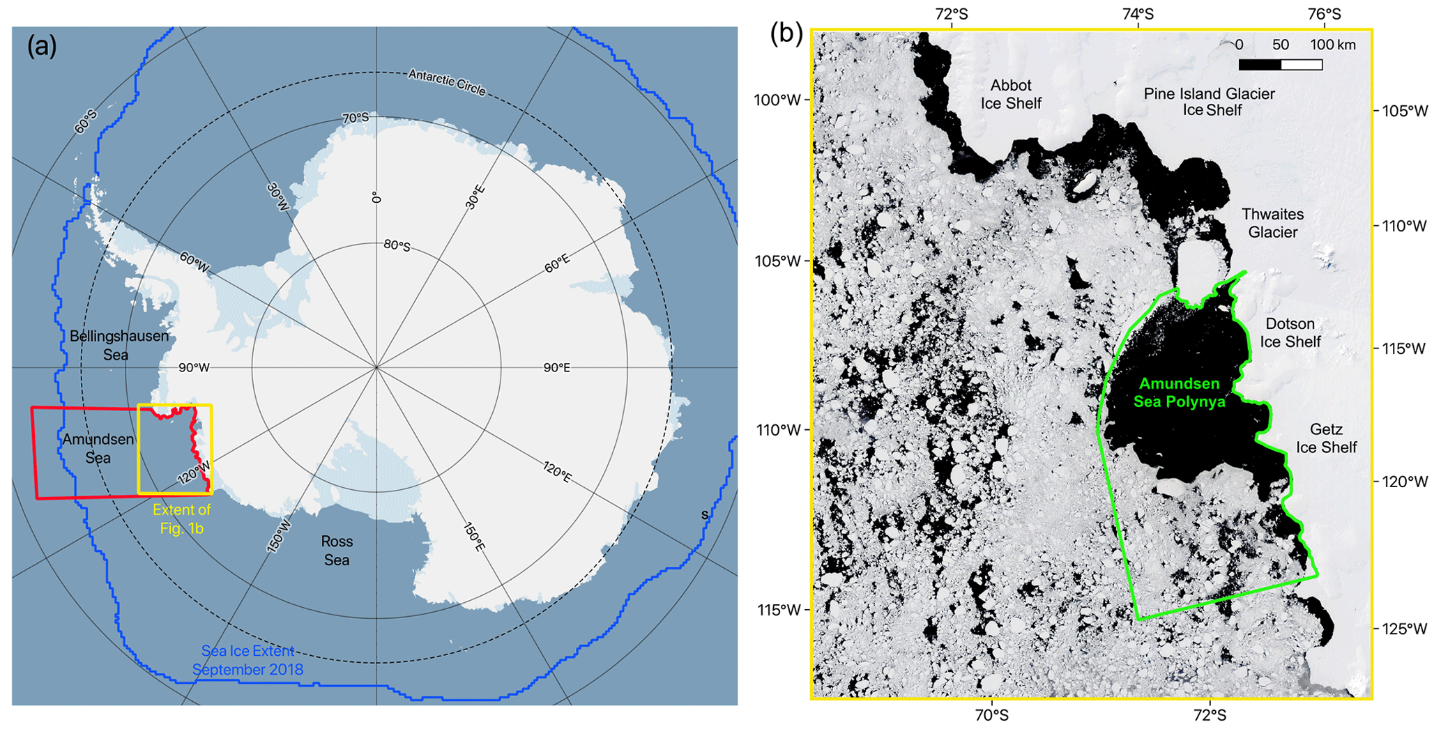
Figure 1(a) The location of the Amundsen Sea and our study sites within the context of Antarctica and the Southern Ocean. The background image is from Quantarctica (Matsuoka et al., 2021); (b) the location of the ASP within the Amundsen Sea Embayment. The green boundary indicates the area defined as the ASP study area for the purpose of calculating the winter polynya area and ice production. The background image is a true-color MODIS image from 12 December 2020.
3.1 Qualitative analysis of the ASP's evolution
In order to qualitatively characterize the seasonal and interannual evolution of the ASP, we use Sentinel-1 SAR imagery. Qualitative visual analysis allows us to identify dynamics that are not easy or possible to identify and/or describe with quantitative data. Sentinel-1 is a constellation of two satellites, A and B, that were launched by the European Space Agency (ESA) in 2014 and 2016, respectively. The satellite collects radar backscatter imagery in the C-band, which allows observations of sea ice and the ocean during cloudy conditions and the polar night.
For our analysis we produced a time-lapse animation in Google Earth Engine using all Sentinel-1 extra-wide swath (EW) mode, Ground Range Detected (GRD) images over the study site, described in Sect. 2, and its surroundings for the period November 2016 to March 2021. This period was chosen because it includes all the complete summer (November–March) and winter (April–October) periods during which both satellites A and B of the Sentinel-1 SAR constellation have been active. The EW mode was primarily designed for sea ice and polar zones and collects images over a wider area than other modes. EW images are available in 20 m×40 m spatial resolution, and all images were resampled to 40 m grid spacing. Of four available band combinations (VV, HH, VV+VH, and HH+HV), we use the HH band because most of the images contain this band. Google Earth Engine applies a series of pre-processing steps to Sentinel-1 images (https://developers.google.com/earth-engine/guides/sentinel1, last access: 1 October 2022): (1) application of orbit file, (2) GRD border noise removal, (3) thermal noise removal, (4) radiometric calibration, and (5) orthorectification. Images are also converted to decibels (dB). Using these images, we created a time-lapse animation using Google Earth Engine. This time-lapse included at least partial coverage of the study area for 56 d in 2016, 359 d in 2017, 341 d in 2018, 317 d in 2019, 329 d in 2020, and 85 d in 2021. In order to analyze particular images in detail, the images were also downloaded from the Alaska Satellite Facility (https://asf.alaska.edu/, last access: 1 November 2021) and processed in ESA's SNAP toolbox. SNAP was used to crop the images, apply radiometric correction (gamma nought), apply a Lee (7×7) speckle filter, and perform ellipsoid correction and map projection, projecting to an Antarctic polar stereographic projection. These images were also converted to decibels. The images were then loaded into QGIS (https://www.qgis.org, last access: 1 November 2021) for analysis.
Qualitative analysis was carried out by visually analyzing the time-lapse videos and images of interest, noting changes in the state of the polynya and ice in the region. Visual analysis is possible by analyzing changes in the backscatter signal's texture, pattern, and tone and because of the distinct backscatter characteristics of open water, older ice pack, and different types of thin sea ice. The motion of the ice between images also helped in the identification of polynya events. Numerous previous studies have noted the ability to observe polynya activity and visually identify polynya opening and the drift of ice with SAR imagery and Sentinel-1 in particular (e.g., Hollands and Dierking, 2016; Dai et al., 2020; Moore et al., 2021). Visual qualitative analysis of SAR imagery also forms an important part of, for example, Environment Canada's production of sea ice charts (Environment Canada, 2005). Typically, open-ocean water has a low backscatter and appears dark, while thicker, older ice pack has a relatively high backscatter and appears bright and more granular (we refer to all ice not produced by the ASP as “pack ice”) (Fig. 2a–b). Recently formed polynya-produced ice has an intermediate backscatter (Fig. 2a). Frazil ice, which may form when a polynya opens up and the open ocean begins to freeze, typically forms in distinct bands of varying brightness (Fig. 2c–d), although it may also form in a swirl or other forms. The open ocean may also appear bright during high winds, but it is typically clear from the pattern, tone, and texture, as well as the context of the image, whether it is an area of ice-free open ocean or an area of pack ice or active polynya. Incidence angle also influences backscatter and should be considered particularly in a quantitative study of backscatter, but it is not generally considered a significant impediment in the ability to qualitatively analyze the images for this study's purpose, with visual analysis dependent on a number of factors. Note that what we refer to as the “active” polynya area during the winter will typically be filled with thin, newly forming frazil ice.
Given the role grounded icebergs play in bounding the ASP, we also downloaded the BedMachine Antarctica V2 seafloor topography dataset for our study area to examine alongside our qualitative analysis. This dataset was downloaded from the NSIDC (https://nsidc.org/data/nsidc-0756) and has a grid spacing of 500×500 m (Morlighem, 2020; Morlighem et al., 2020).
We also use our analysis of the imagery to assess the approximate day of summer polynya “opening” and “closing”. We deem the polynya to be open for the summer when the open polynya area is primarily free of active ice production, and we deem the day of summer closing to be when the whole open polynya is subject to ice production.
3.2 Daily polynya area
In order to analyze seasonal and interannual changes in polynya area in summer and winter, daily sea ice concentration (SIC) for the study region was downloaded from the University of Bremen's sea ice data center (https://www.seaice.uni-bremen.de, last access: 18 May 2021). The data were separated into five summer periods from November to March (2016/17, 2017/18, 2018/19, 2019/20, and 2020/21) and four winter periods from April to October (2017, 2018, 2019, and 2020). This time period was focused on because it coincides with the period for which there are Sentinel-1 A and B data. During the winter we use the term “active polynya” for areas that we include in the polynya, where an opening has been created and new ice production is taking place. During the winter we expect thin, frazil ice to immediately begin forming when an opening is created (e.g., Nakata et al., 2019, 2021), and thus we prefer the term “active” to “open” polynya. We begin our winter period in April rather than March because analysis of the Sentinel-1 imagery suggests ice production is not typically active across the open polynya at the beginning of March. The sea ice concentration product was processed by the University of Bremen using the ARTIST Sea Ice (ASIC) algorithm (Spreen et al., 2008) applied to AMSR-2 data. AMSR-2 was launched aboard the Japan Aerospace Exploration Agency's (JAXA) Global Change Observation Mission – Water (GCOM-W) satellite in July 2012.
We used version 5.4 of the Antarctic-wide, daily sea ice concentration product with no land mask, processed to 3.125 km grid spacing. This is of a higher resolution than data previously used to analyze polynya area in the region. For example, Arrigo et al. (2012) used SSM/I data with 6.25 km grid spacing for their study of summer polynya area. Nihashi et al. (2017) used AMSR-E data with 6.25 km grid spacing for their estimates of ice production. Tamura et al. (2008, 2016) also used SSM/I data, with 12.5 km grid spacing, for estimates of ice production. Stammerjohn et al. (2015) used bootstrap SIC data with 25 km grid spacing for their analysis of summer polynya area. However, with our higher-resolution data (3.125 km) there remain limitations in using data with such a scale to measure something that can vary on a meter scale. It has been estimated that the ice concentration error in our AMSR-2 dataset is 25 % at 0 % SIC, decreasing to <10 % error for SIC over 65 % and 5.7 % error at 100 % SIC (Spreen et al., 2008). It is also noted that the SIC data are known to underestimate SIC where there is thin ice, but as we define an active polynya as including thin ice, this is not likely to lead to substantial misclassification of active polynya areas. The data may also incorrectly classify stable fast ice as being an area of low SIC, but we exclude these areas from the study area. Data were available for all days in our study period apart from 1 d in 2019 (1 September).
After each day's data were downloaded as a GeoTIFF file, they were cropped to the 70 660 km2 ASP study area defined in Fig. 1b using a shapefile drawn in QGIS with a Sentinel-1 image as reference. Polynya area was then calculated by defining any pixel in the study area with a SIC <70 % as being part of the open/active polynya. The 70 % threshold has been commonly used in other studies of polynyas in the summer (e.g., Parmiggiani, 2007; Morelli and Parmiggiani, 2013; Preußer et al., 2015), and the approach has also been used before to calculate winter polynya area (Cheng et al., 2017, 2019). A limitation is that smaller areas of open water that are represented in a pixel dominated by ice-covered area (i.e., >70 %) will not be included in our polynya area value, while ice-covered areas in pixels with SIC <70 % will be included. However, by comparing our SIC data with the SAR imagery, we found applying a 70 % threshold to the SIC data to be an effective way of capturing winter, as well as summer, polynya area in our study area. For example, Fig. 2b–d show SAR imagery for a section of the polynya on 21–23 September 2020, and Fig. 2e–g show the active polynya as identified using a 70 % threshold with the SIC data for the same days. To further compare the identification of active winter polynya as identified using SIC data with the SAR imagery, we manually identified active polynya in the SAR imagery for the nine dates in 2020 when SAR imagery covers the whole ASP study area (green box in Fig. 1b). The results of the comparison can be seen in Fig. S1 in the Supplement and generally show good agreement. Note that even if the method was perfect there would be a discrepancy because the measurements are taken at different times of day, and significant changes in active area can occur in hours due to movement of ice, freezing, or a mixture of processes. There is also an element of human error in the manual measurement. Of the nine cases, the area was identified as higher using SIC data in five cases and using SAR data in four cases, suggesting that neither approach leads to a systematic overestimation. Observing Video S2 in comparison to available images in Video S1 also shows the SIC typically effectively captures the presence and variations in area of the active polynya.
While Sentinel-1 imagery has been used to obtain polynya area during the polar night at a higher spatial resolution (40 m, Dai et al., 2020), the Bremen SIC product has three key advantages over using Sentinel-1 SAR imagery. First, the SIC product is available daily, in contrast to Sentinel-1, which has many, and sometimes prolonged, data gaps over the primary area of interest, particularly during June/July. Given that polynya area can change substantially on a daily or hourly timescale, regular gaps of successive days significantly limit the ability to quantitatively characterize variations throughout the year. Second, several Sentinel-1 images are required to capture the whole ASP study area on a particular day, meaning that even on many days where there are images that are useful for qualitative analysis, the whole polynya cannot be measured. For example, in 2020 there is full coverage of the whole ASP study area for only 22 d, with none between 26 April and 12 August, and 9 d in winter (although there are many other days when the whole of the actual open/active polynya itself is visible as it does not extend throughout the whole study area). Third, even if sufficient images were available, current methods for calculating polynya area in Sentinel-1 imagery (e.g., Dai et al., 2020) require manual delimitation, which is labor-intensive and would be highly time-consuming to do for multiple years at a daily temporal resolution. Automated detection of active polynya area in winter using SAR is not yet possible to our knowledge.
3.3 Daily winter ice production
In order to calculate daily ice production in the ASP during the winter periods, we followed the approach of Cheng et al. (2017) and utilized their heat flux and ice production model. As input to the model, we used atmospheric reanalysis data from the European Centre for Medium-Range Weather Forecasts Reanalysis v5 (ERA5) and the same sea ice concentration data from the University of Bremen described in Sect. 3.2.
Hourly ERA5 data, with a spatial resolution of 31 km, were downloaded from Copernicus (https://cds.climate.copernicus.eu, last access: 21 April 2021; Hersbach et al., 2018) for the following meteorological variables: air temperature at a height of 2 m, wind speed at a height of 10 m, surface air pressure, dew point temperature at a height of 2 m, downward solar radiation, and downward thermal radiation. Air temperature, wind speed, surface air pressure, and dew point temperature were then processed to daily mean values, while solar and thermal radiation were processed to daily cumulative values. These calculations were done for the same ASP study site as for polynya area (Fig. 1b).
3.3.1 Heat flux calculation
Following Cheng et al. (2017), the daily net heat flux, Q (in W m−2), of an active-polynya pixel was estimated by
where Ri (in W m−2) is the cumulative downward solar radiation; Li (in W m−2) is the cumulative downward thermal radiation; Lo (in W m−2) is the upward thermal radiation; Fs (in W m−2) and Fe (in W m−2) are the sensible heat flux and latent heat flux, respectively; and α is the albedo of open water. α was taken to be 0.06 following Cheng et al. (2017, 2019); Ri and Li were taken from the processed daily ERA5 values; and Lo, Fs, and Fe were calculated as described below.
The upward thermal radiation was calculated by the Stefan–Boltzmann law:
where ε is the longwave emissivity of open water (0.99), and σ is the Stefan–Boltzmann constant ( W−2 K−4). The temperature of the water surface (Ts, in K) was assumed to be at the freezing point of seawater (T0 in K), which was calculated following Doherty and Kester (1974) and Cheng et al. (2017, 2019) as
where Sw (in ‰) is the salinity of seawater. The salinity of the Amundsen Sea was estimated as 34 ‰ based on Bett et al. (2020).
The sensible heat flux (Fs) and latent heat flux (Fe) were calculated by
and
where ρa is the density of air at standard atmospheric pressure and 0 ∘C, taken as 1.3 kg m−3; cp is the specific heat of air at constant pressure, taken as 1004 J kg−1 K−1; U (in m s−1) is the wind speed at 10 m, taken from the processed ERA5 data; and Ta (in K) is the air temperature at 2 m, taken from the processed ERA5 data. Cs and Ce are bulk transfer coefficients for sensible heat and latent heat, respectively, both taken as 0.00144. P0 (in Pa) is the surface air pressure and taken from the processed ERA5 data. Lv (in J kg−1) is the latent heat of water vaporization; r is the relative humidity. ea (in Pa) is the saturation water vapor pressure at the air temperature, rea is the actual water vapor pressure of the air, and es (in Pa) is the saturated water vapor pressure at the surface temperature and are all calculated below:
and
where Td is the dew point temperature taken from the processed ERA5 data.
3.3.2 Ice production calculation
The calculated daily heat flux was then cropped, realigned, and resampled to a 3.125 km2 grid and reprojected to Antarctic Polar Stereographic using GDAL (Geospatial Data Abstraction Library) and QGIS to match the corresponding sea ice concentration data. Next, where SIC was <0.7 (i.e., pixels considered as part of active polynya), daily ice production volume, V, was estimated in cubic kilometers (km3) following Cheng et al. (2017) by the following Eq. (9). Although ice production will also take place in non-polynya areas where there is ice cover, here we are only concerned with ice production taking place in the active polynya.
where, as above, SIC is sea ice concentration (as a fraction) and Q is daily net heat flux in watts per square meter (W m−2), ρi is sea ice density and taken as 920 kg m−3, and Lf is the latent heat of sea ice fusion in joules per kilogram (J kg−1). Lf is calculated following Mohammed and Nirmal (2015) and Cheng et al. (2017) by
where Si is the salinity of sea ice, taken as 6 ‰ following Cheng et al. (2017).
Caution should be used when interpreting the absolute numbers produced by the ice production model, particularly because the input data are reanalysis data not necessarily always representative of reality. This is so because the reanalysis itself is a simulation sensitive to uncertain parameter settings, although it is partly corrected by assimilation of observational data (Cheng et al., 2017, 2019). Also note ERA5 includes a prescribed “sea ice area fraction” parameter that influences the interaction between the atmosphere and ocean in the reanalysis. Nevertheless, we opted for this method due to the difficulty of directly measuring and tracking thin ice thickness in the polynya (e.g., Tian et al., 2020) to estimate ice production, as well as the potential to compare our daily ice production results to results obtained by the same model for the Ross Ice Shelf Polynya (Cheng et al., 2017, 2019).
3.4 Broader spatial changes in SIC
In order to assess changes in the ASP in the context of changes in SIC at a broader spatial scale, SIC was analyzed for the larger area defined in Fig. 1a. The same SIC dataset described in Sect. 2.2 to obtain polynya area was cropped to the broader region. The daily data were plotted spatially for all the available days of 1 November 2016–31 March 2021, as shown in Video S2. Monthly mean SIC was also calculated for the whole period and plotted spatially. Additionally, the total SIC for each day was calculated by calculating the sum of all percentage SIC values in the study region. These total SIC values should only be considered useful for analyzing relative changes in SIC in our study period.
3.5 Wind analysis
In order to analyze the polynya's behavior, we also considered wind conditions. Although a thorough analysis of wind-vector/ice property correlations is beyond the scope of the present paper, which is primarily focused on estimating and describing the variability of the polynya's dynamics, area, and ice production, we do consider wind conditions to help inform our analysis of the polynya. Mean daily and annual wind speed and vector winds were calculated from hourly ERA5 reanalysis wind products. Hourly zonal (u) and meridional (v) components of vector winds at a height of 10 m were obtained from ERA5 for a region adjacent to the Dotson Ice Shelf and Iceberg Chain where the polynya typically forms, identified in Fig. S2. Hourly wind speed (V) in meters per second (m s−1) and wind direction (θ) in degrees were calculated as
and
respectively. Daily averaged vector wind fields superimposed on maps of daily averaged wind speed were plotted for the whole study area for the period 1 November 2016 to 31 December 2020 and are included as Supplement Video S3. A wind rose (Fig. 8) showing the wind speed and direction at times when the active polynya both did not and did increase in area during winter (2017–2020) was also produced for the smaller area (shown by Fig. S2) where the polynya forms from. A map of annual mean vector wind field superimposed on a map of annual mean wind speed was plotted in Fig. 9.
Unfortunately, there is a lack of local observations of wind data in and around the study area, with the closest station in the United States Antarctic Program's database, on Bear Peninsula, lacking wind data for most of our study period. As a result, some caution should be employed when considering the results obtained from ERA5 winds. However, Bracegirdle (2013) and Stammerjohn et al. (2015) note that data from ERA5's predecessor ERA-I in the neighboring Bellingshausen Sea performed better than other reanalysis products.
In this section, we first summarize our qualitative analysis of the polynya dynamics using Sentinel-1 SAR imagery (Video S1) of the ASP between November 2016 and March 2021 (Sect. 4.1). Second, we analyze quantitative changes in summer (November–March) polynya area for the summers of 2016/17 to 2020/21 (Sect. 4.2). Third, we analyze quantitative changes in winter (April–October) polynya area and ice production for the winters of 2017 to 2020 (Sect. 4.3). Fourth, we analyze spatial and temporal wind variations and how they relate to polynya area (Sect. 4.4), and finally we analyze broader regional patterns in sea ice concentration for the period November 2016–March 2021 (Sect. 4.5).
4.1 Qualitative analysis of ASP using Sentinel-1 SAR imagery
Typically, in November or early December the polynya transitions from a winter into summer mode as it expands to the west and ice production ceases to take place in the open area; i.e., the open polynya area is occupied by open ocean rather than frazil or grease ice (Table 1, Video S1, e.g., Fig. 1b). While the polynya's eastern and southern boundaries remain fixed at the Iceberg Chain and coast, respectively, at times during the summer the polynya becomes unbound to the west and/or north and consequently congruent with the open ocean. In the summers of 2018/19 and 2019/20 it remains bound, but in 2016/17 and 2017/18 substantial openings develop in the pack ice boundary. In the summer of 2016/17, particularly from December, the pack ice in the region is notably sparse in comparison to the other years.
In February the pack ice around the polynya becomes more extensive and compact, predominantly due to inflow from the Bellingshausen Sea in the northeast. As the new pack ice flows into the area it reforms a western/northern boundary to the polynya in the years where a gap had opened and in all years pushes the existing pack to the east and southeast, reducing the polynya's size. In the exceptionally low pack ice summer of 2016/17, the newly formed boundary of pack ice is remarkably narrow. In March in all years, new ice production can be seen forming in parts of the polynya and is taking place across all of the polynya by the end of March or early April, marking the polynya's transition into winter mode (Table 1).
Throughout the winter, polynya events occur, with existing ice moving away, predominantly to the west off the Iceberg Chain and Thwaites Iceberg Tongue, and new ice forming in the opening (e.g., Fig. 2b–d). On occasion the polynya instead forms to the north off the Dotson Ice Shelf. Between April and August, the main polynya appears to primarily have its maximum extent confined to the area adjacent to the Dotson Ice Shelf. Observation of available imagery of polynya events, along with observation of newly formed polynya ice outflowing from the area, suggests that there is relatively low ice production in these deep winter months. Early and late in the winter, polynya events are sometimes larger, extending further to the west, and there appears to be more associated ice production.
After early winter (March–April), as the area becomes more densely covered by inflowing pack ice and newly formed polynya ice, obstructions occur that appear to limit the evacuation of polynya-produced ice from the vicinity and limit growth of the polynya. Obstructions particularly take place around and adjacent to a group of persistently stuck icebergs around the center of the study area that we call the Central Grounded Icebergs around a seafloor high (Fig. 2a, h). New ice also sometimes becomes stuck (fast) directly adjacent to the southwest of this site (Fig. 2a, h) on another seafloor high. This intermittently fast ice blocks outflow from the polynya to the west along the coast and at times forces new polynya-produced ice to divert around the north of Central Grounded Icebergs (Fig. 2a). An area of grounded icebergs and intermittently fast ice by Siple Island also sometimes obstructs ice and causes diversions further to the north. All ice produced by the polynya flows to the west overall, eventually rounding the corner of Siple Island.
We also observe that, while the overall flow of ice from the ASP is to the west, ice flowing from the polynya through the winter heaves and regularly temporarily reverses direction, backfilling eastward into and towards the polynya (e.g., Fig. 3). This means the polynya sometimes closes through backfilling and not only through formation and growth of new ice. Backfilling also occurs when the polynya does not appear open, meaning that rafting and deformation presumably occurs as ice moves back into the polynya zone.
A series of smaller polynyas, other than the main polynya that forms off the Iceberg Chain and Dotson Ice Shelf, also form within the study area at times. Mostly notably a “secondary polynya” forms at times off the Central Grounded Icebergs (Fig. 2a). With inflow of ice from the ASP to this area at times obstructed, as ice moves away from the Central Grounded Icebergs to the west, an opening is created and active ice production is visible. Small polynyas also form at times to the west off the outcrops along the coast.

Figure 2An example image of the ASP during the winter in a Sentinel-1 SAR image from 5 September 2019. (b–d) An example of an active polynya event taking place on 21–23 September 2020 in Sentinel-1 SAR imagery. Darker ice produced by the ASP can be seen diverting around the Central Grounded Icebergs (and some fast pack ice) after ice became stuck and obstructed outflow along the coast. The area corresponds to the dashed green box in panel (a). (e–g) Active polynya area (blue) for the same dates and areas as panels (b)–(d), as measured by using a 70 % threshold with SIC data. (h) The elevation of the bed referenced to mean sea level for the same area as panel (a). The bathymetry data are from the MEaSUREs BedMachine version 2 dataset (Morlighem, 2020).
Table 1Summer polynya opening and closing dates for each summer 2016/17–2020/21 as determined by visual analysis of Sentinel-1 SAR imagery. We determine the polynya to be open for summer when the majority of the open polynya is not exhibiting ice production and closed when the majority of the polynya is exhibiting ice production. * In 2016/17 a lack of imagery in early November means it is difficult to determine when the polynya opened, but it is open by 8 November.
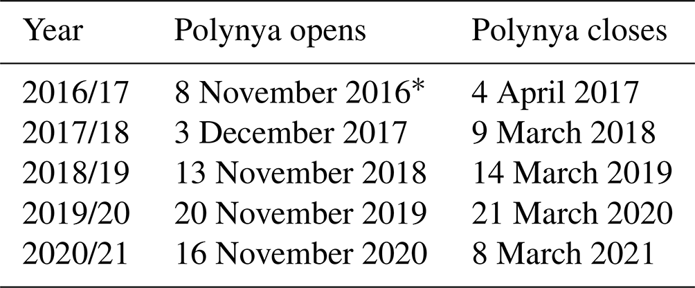
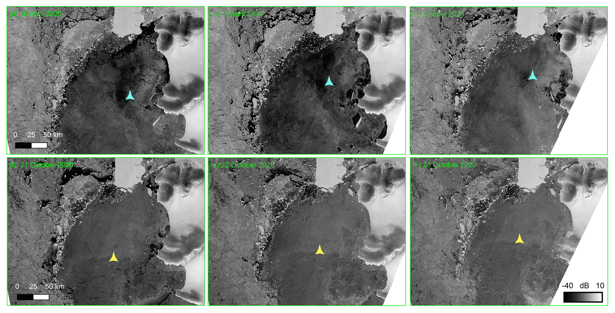
Figure 3Examples of backfilling ice earlier produced by the ASP flowing back towards the area adjacent to the Iceberg Chain where it formed. Each box corresponds to the same area shown by the dashed green box in Fig. 2a; panels (a)–(c) show the area on 18–20 April 2020; panels (d)–(f) show 21–23 October 2020. The colored shapes in each image are in approximately the same relative position within the ice in each set of images and are to help the reader spot the movement of the ice through the movement of adjacent features. Other examples of backfilling are visible in Video S1.
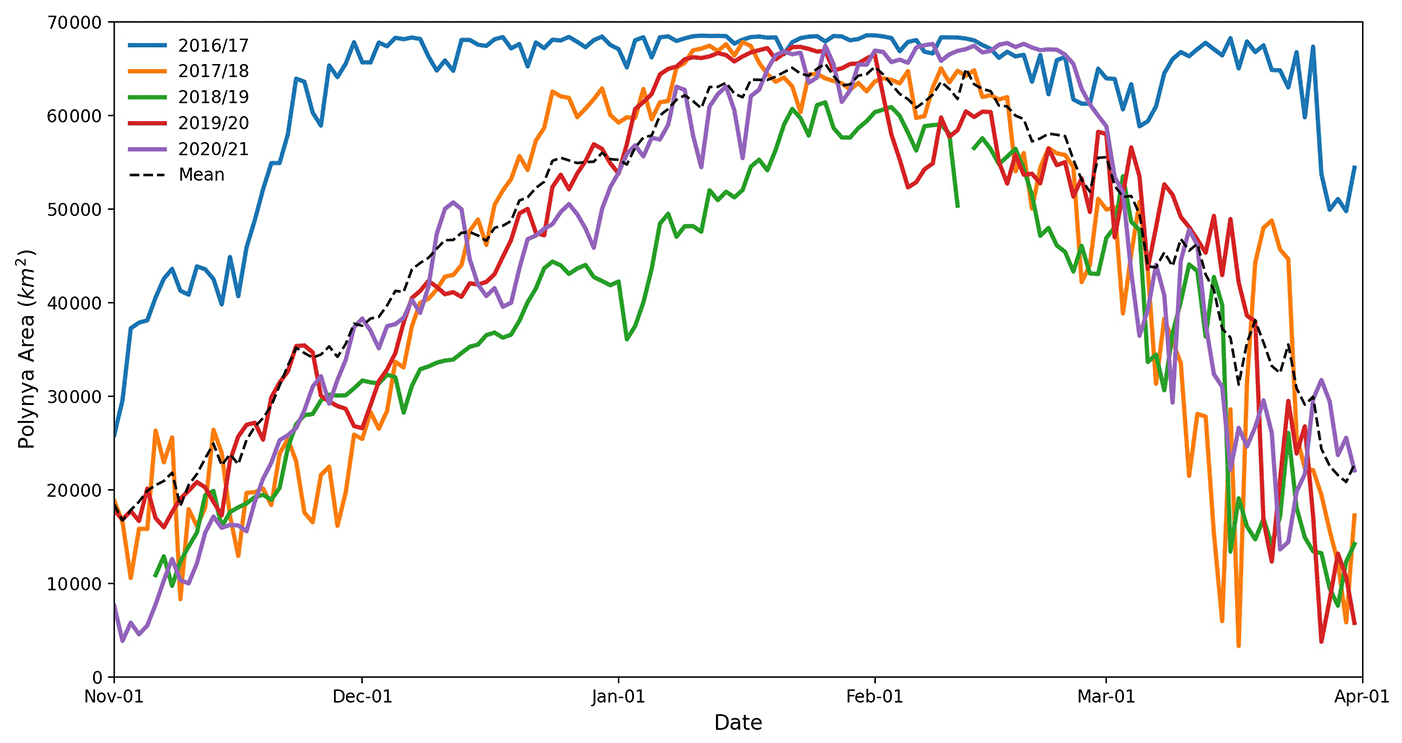
Figure 4Daily summer (November–March) polynya area for each summer 2016/17–2020/21 (solid), and the 5-year mean of the daily areas for the whole summer period (dashed).
4.2 Summer polynya area
In all years there is an overall increase in polynya area through November (Fig. 4). On 1 November, the polynya has an area between 7617 km2 (2020) and 25 859 km2 (2016). In the years 2017/18, 2018/19, 2019/20, and 2020/21 the polynya area follows a similar pattern, but in 2016/17 it follows a distinct course. By 1 December in 2016 the polynya is open in approximately the whole ASP study area, with an area of 65 674 km2, an increase of 154 % from 1 November. In 2016/17 the polynya remains open across approximately the whole study area throughout December, January, and most of February and March, only beginning to significantly decline in late March (Fig. 4) and into April (Fig. 5). The polynya in 2016/17 maintains a higher area than in all other years throughout the whole summer, apart from a small period in late February when it is surpassed by 2020/21.
In 2017/18, 2018/19, 2019/20, and 2020/21 the polynya area has increased to between 25 439 km2 (2017) and 38 310 km2 (2020) by 1 December. From then the polynya continues to follow an overall increasing trend through December, with the polynya reaching its peak area in January in each of these years. In 2018/19 the peak area is substantially lower (61 113 km2) than in other years, and the polynya only maintains an area above 60 000 km2 for 6 d in late January and early February. 2018/19 records the lowest area in comparison to other years on every day between 4 December and 3 February. In 2017/18, 2019/20, and 2020/21 the polynya behaves in a similar manner through most the period, with no one of those years consistently recording a higher area and each year reaching a peak-open area that approximately fills the whole ASP study area. However, polynya area in 2020/21 reaches its peak later (January), and its decline begins later (late February). Notably, in 2017/18 the polynya experiences a temporary rapid reopening as it increases from just 5977 km2 on 15 March to 48 779 km2 on 21 March. This is an 8.2-fold increase in 6 d, and it is followed by a rapid decline. The polynya had the highest daily mean area for summer (November–March) in 2016/17, at 62 616 km2, and 2018/19 had the lowest, at 38 518 km2. The mean daily area of 2017/18, 2019/20, and 2020/21 for summer was 44 013, 44 979, and 44 447 km2, respectively.
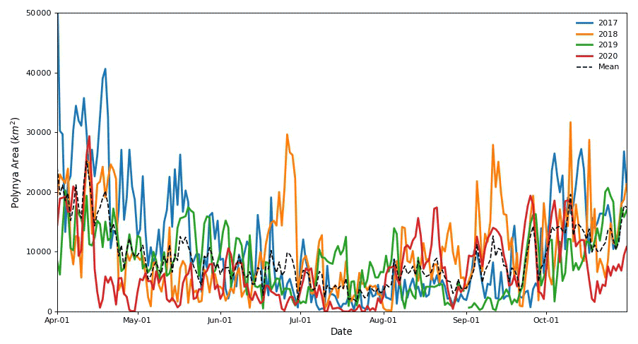
Figure 5Daily winter (April–October) polynya area for each winter 2017–2020 (solid), and the 4-year mean of the daily areas for the whole winter period, as measured from AMSR-2 SIC data (dashed).
4.3 Winter polynya area and ice production
In all years, polynya area exhibits an overall decline from the beginning of the winter period, when the polynya remains relatively large after the summer period (Fig. 5). This period, when the polynya remains relatively large but ice production has now begun, accounts for a substantial proportion of the annual ice production (Figs. 6, S4). On average, April–May accounts for 36 % (39.6 km3) of annual ice production. The polynya then generally reaches a sustained winter low in area, where it fluctuates around and below 10 000 km2. In 2020 the polynya area reaches its low in early April, while in 2017, 2019, and the mean for 2017–2020 the area continues an overall decline through April, May, and June. Polynya area and ice production then tend to remain low until an increase begins around September. In July polynya area remains below 10 000 km2 in all years for the whole month, apart from brief small fluctuations above this in 2018 and 2019. There are notable spikes in polynya area in the middle of the year, which are also exhibited in spikes in ice production. Most notably in June in 2018 polynya area spikes to 26 631 km2. After a period of low polynya area, the area generally increases through September and October towards the summer period. In 2020 this period of area and ice production increase begins in August. This late-winter increase in polynya area is also exhibited in a corresponding marked increase in the rate of ice production. On average, September–October accounts for 42 % (45.8 km3) of annual ice production.
We note that in 2017 between the dates of 1 April and 8 May a substantial portion of the calculated active polynya area and ice production occurs in the northwest of the ASP study area. This area is part of the open ocean and is separated by sea ice from the more typically active polynya area adjacent to the Iceberg Chain. Typically, ice pack fills this northwest area, but in early 2017 it is open due to the lack of ice pack in this sector in the summer of 2016/17, discussed in Sect. 4.3 (Video S2; Fig. 11b).
Analysis of the spatial distribution of ice production across all years reveals that the mean daily ice production is highest in the area of the polynya adjacent to the Iceberg Chain, Thwaites Iceberg Tongue, and Dotson Ice Shelf (Fig. 7). Mean annual ice production values (April–October) in this region surpass 17 m3 m−2. Other notable areas of higher ice production lie along various parts of the coast and an area that corresponds to the secondary polynya by the Central Grounded Icebergs.
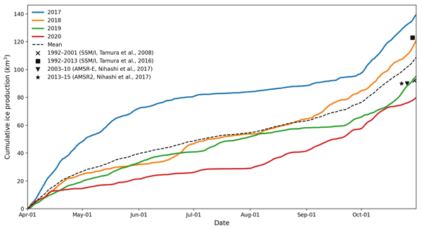
Figure 6Daily cumulative winter ice production for each winter (April–October) 2017–2020 (solid), and the 4-year mean for the period (dashed), as measured using heat flux modeling of ERA-5 data and AMSR-2 SIC data. Also shown are mean annual measurements for 1992–2001 (Tamura et al., 2008), 1992–2013 (Tamura et al., 2016), and 2003–2010 and 2013–2015 (Nihashi et al., 2017), along with the instrument used for each measurement. Note the previous studies' measurements covered the period March–October and used a study area that does not exactly correspond to ours.
Table 2Estimates of mean daily active polynya area, total annual ice production, and mean daily ice production during the winters of 2017–2020 and for the daily mean of the period. Numbers in brackets indicate the standard deviation.
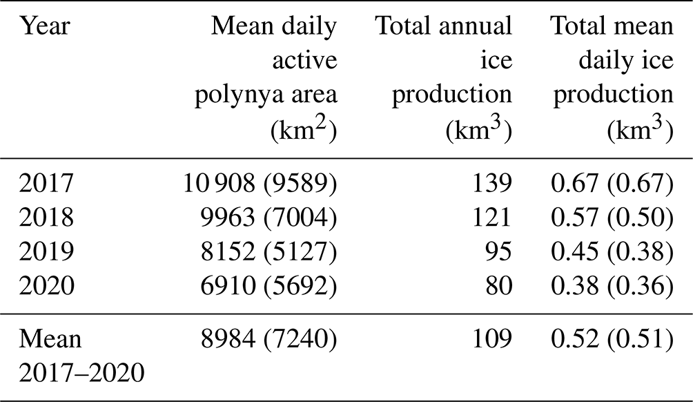

Figure 7Mean annual ice production for all winter study periods (April–October 2017–2020). The region corresponds to the region within the green outline in Fig. 1b.
4.4 Wind and polynya area
Polynya events are associated with the presence of strong southeasterly and easterly winds in the region. Figures 8–9 show that southeasterly and easterly winds dominate the polynya study area. Comparing winter winds, in the region where the polynya forms from (Figs. 8, S2), when the active polynya does not increase in area and when it does, shows that while southeasterly winds often occur in both instances, there is a stronger easterly component when an increase in area occurs. The top three wind directions associated with a daily increase in active polynya area are southeasterly, east-southeasterly, and easterly, whereas they are southeasterly, southerly, and south-southeasterly when area does not increase. Figure S3 also shows the high density of active polynya area increases with winds with a southerly/easterly winds. It is also visible in Fig. 9 that the location of polynya formation, adjacent to the Dotson Ice Shelf, is associated with a band of high winds with a mean speed of around 8–9 m s−1 that extends along the coast from Thwaites Glacier, over the Thwaites Iceberg Tongue, and into the southeastern area of the ASP study area. In the western part of the study area that the polynya extends into, winds tend to be more easterly than southeasterly.
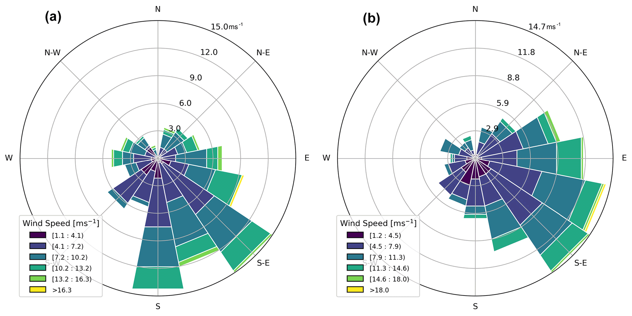
Figure 8Wind roses showing the distribution of wind speed and direction during all winters (April–October) in the study period, when the active polynya (a) did not increase in area and (b) did increase in area. These winds are calculated for a region close to the Iceberg Chain that the polynya forms from, shown by Fig. S2.
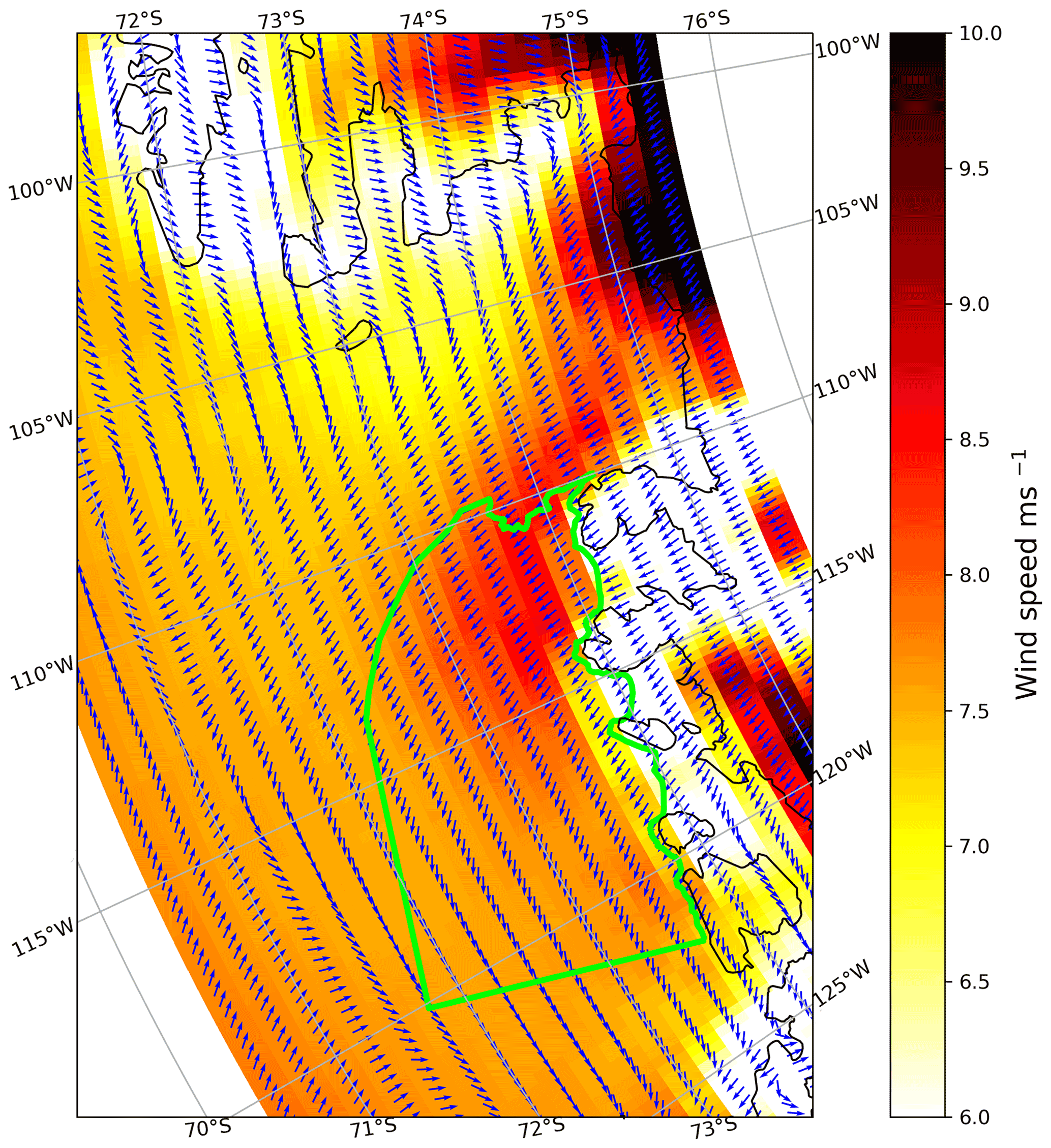
Figure 9Annual mean vector wind field and wind speed, calculated for the period 1 November 2016 to 31 December 2020. The green boundary represents the ASP study area, also shown in Fig. 1b. Daily maps of vector wind fields and wind speed are included as Video S3.
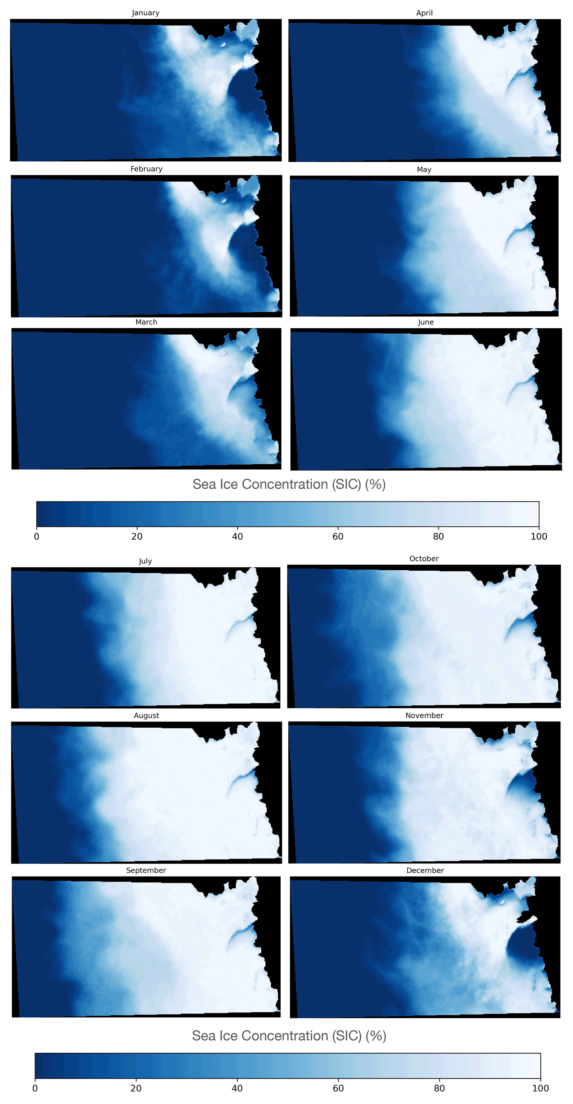
Figure 10Mean monthly SIC for the broader ASP region for the period November 2016 to March 2021. The area corresponds to that shown by the red box in Fig. 1a. Daily data are shown in Video S2.
4.5 Broader SIC
Analysis of the SIC over a broader area also shows daily changes in the polynya area and how it relates to changes in the ice pack. The mean monthly cycle of the polynya can be seen in Fig. 10 and presents a similar picture of the polynya as described in Sect. 4.1–4.3. The broader ice pack has a minimum total SIC in January and remains similar in February. From March the broader ice pack can be seen to expand in area as the polynya begins to close and continues to increase until a peak SIC in September. From October the ice pack begins a marked decline into summer. Interannual variation can be seen in Fig. S5 and Video S2, with maximum ice pack area occurring in August or September each year and minimum ice pack in January or February.
During the summer of 2016/17 the ice pack is notably sparse (Figs. 11, S5). Around 29 December 2016 a gap in the ice pack connects the ASP to the open ocean to north. The ice pack continues to diminish and the gap connecting the ASP to the open ocean broadens until by February the polynya is only bound by part of the Iceberg Chain and Thwaites Iceberg Tongue. The total SIC reaches a minimum on 5 February 2017, 35 % of the next lowest annual minimum (2019/20). Gaps in ice pack around the Iceberg Chain mean that the ASP has essentially joined with the Pine Island Polynya through the Iceberg Chain for a period in this year. The narrow band of ice pack from the east closes the polynya off again in March, but the band of adjacent ice pack remains so narrow that, as mentioned, there is open ocean inside our ASP study area until 9 May (Video S2).
Our analysis shows that in some ways the ASP, between November 2016 and March 2021, behaves as is typical for Antarctic coastal polynyas. During the summer the polynya becomes larger and remains ice-free (Fig. 4, Video S1), while during the winter it becomes smaller, activating during ice-producing polynya events (Figs. 4–5, Video S1). These polynya events and changes in polynya area can sometimes be attributed to higher wind speeds and are often associated with a stronger easterly component in winds close to the Iceberg Chain (Figs. 7–9, S3).
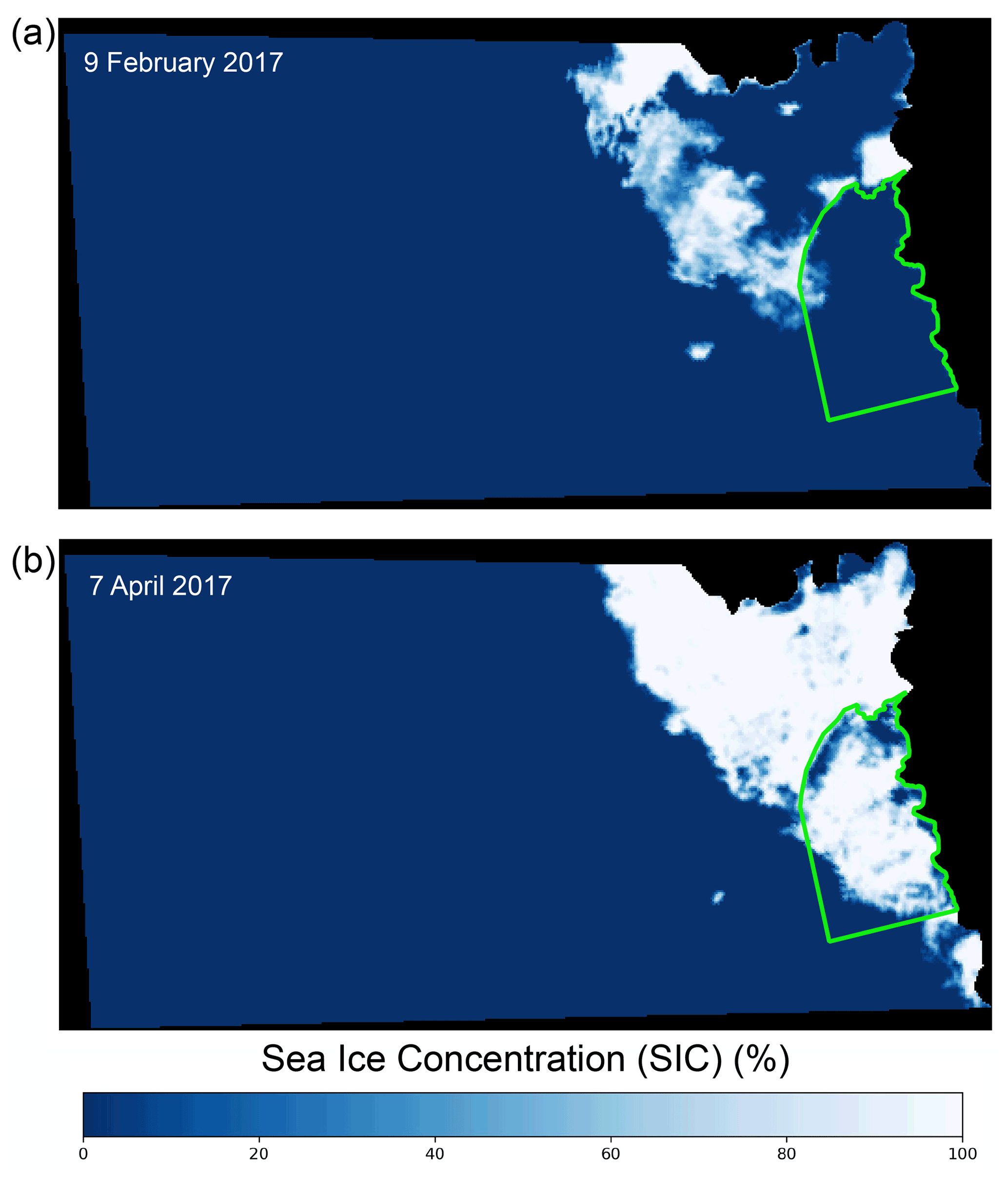
Figure 11SIC for the broader ASP region on two dates in 2017, during and following a summer of record-low SIC. (a) An example of when the polynya had no sea ice boundary to the west/northwest due to the exceptionally low SIC in the region during the 2016/17 summer. (b) An example of the low SIC in the region early in the subsequent winter, when only a narrow area of pack ice and polynya ice fills the area. The area corresponds to that shown by the red box in Fig. 1a.
Our qualitative analysis of Sentinel-1 SAR imagery, however, also reveals distinct characteristics of the ASP which are not possible to decipher from sea ice concentration data, other quantitative methods, or indirect observation. First, we note that while in many other polynyas, such as the Ross Ice Shelf Polynya, new polynya-produced ice is typically efficiently evacuated away from its origin (Dai et al., 2020), this is not the case at the ASP. Instead, ice formed by the ASP often remains in the ASP study area for months (Video S1). In fact, this polynya-produced ice does not consistently flow in a direction away from the polynya. While its overall direction is westward, away from the polynya, the ice heaves and temporarily flows backward (backfills) (Fig. 3), as has also been observed at the Mertz Glacier Polynya (Massom et al., 2017). The ice also gets stuck in the region, particularly around grounded icebergs, which are grounded in areas where there are topographic highs in the seafloor (Fig. 2a, h).
The tendency of ice produced by the ASP to remain in the vicinity of the polynya for prolonged periods, become stuck, and sometimes flow back eastward towards the site of its formation influences the polynya and ice production in two key ways. First, when ice moves back eastward while the polynya is active, it contributes to the closure of the polynya and thus the cessation of ice production. Typically, it is assumed that an active polynya during winter closes due to new ice production (e.g., Cheng et al., 2017). However, the ASP may close both due to ice production and movement of previously produced ice into the polynya. Second, we suggest that the blockages of ice in the vicinity of the polynya reduce the size and frequency of polynya events by hindering the ability of ice to move out of the polynya and open it up. Again, by reducing the size and duration of active polynya area during winter, ice production is limited.
We also note that the ASP forms along the coast westward off a chain of icebergs that extend from the Thwaites Iceberg Tongue. While some polynyas, such as the Ross Ice Shelf Polynya, form off and away from the coast, the majority of Antarctic polynyas have been shown to form westward off glacier ice tongues or protruding fast ice (Nihashi et al., 2017). In the case of the ASP, its location and orientation is determined by the presence of the Iceberg Chain, which is in turn determined by the presence of a bathymetric high (Figs. 1–2). Stammerjohn et al. (2015) refer to the polynya as forming off a “fast ice tongue”, but we prefer to refer to the Iceberg Chain as the eastern boundary. While a section of fast ice exists amongst and adjacent to a section of the southern part of the Iceberg Chain, the extent of this fast ice varies and it only ever extends along a portion of the Iceberg Chain. The Iceberg Chain remains virtually the same length throughout our observations. The polynya consistently forms off the Iceberg Chain regardless of the state or extent of the fast ice. This means that, unlike polynyas that form off variable fast ice (Nihashi et al., 2017), the fundamental morphology of the ASP remains stable through the period. We also note that at no point do we observe significant portions of ice pack to break through the Iceberg Chain from the east, regardless of the state of fast ice extent or conditions, and thus the icebergs and the bathymetric high persistently shield the polynya from ice pack inflow.
Another notable feature of the ASP is the development of a secondary polynya during the winter (Fig. 2a), where ice production also takes place. This is a polynya that forms within the ASP study area, in an area that is usually part of the main ASP during the summer, but it is not typically congruent with the main polynya during the winter. The polynya forms at the site of the Central Grounded Icebergs and associated stuck, transient fast ice. Because some ice has become stuck over the bathymetric high, when adjacent ice drifts away a polynya activates. This feature again highlights the significance of the bathymetry of the region for sea ice production and dynamics.
In line with previous studies of the ASP we find that the ASP is an important site of ice production throughout the winter. Our estimates of annual ice production for 2018, 2019, and the mean for 2017–2020 fall within the estimations by Tamura et al. (2008, 2016) and Nihashi et al. (2017) for 1992–2001, 2003–2010, and 2013–2015 (90–123 km3) (Fig. 6). Our estimates for total annual ice production for 2017 (139 km3) is higher than the highest estimate of those studies, while for 2020 (80 km3) it is lower. This suggests no significant trend in interannual ice production can be discerned from comparing the period of our study to these previous studies. Some caution must be used in this comparison, however, because those studies include March in ice production calculations, and our ASP study area does not exactly correspond to theirs.
We find that the shoulder seasons of April–May and September–October are particularly important for ice production due to the higher polynya area at these times, accounting for 36 % and 42 % of the annual ice production, respectively. This is particularly the case in 2017, when an exceptionally high open polynya area in the summer, due to low ice pack conditions (discussed below), continues into the winter period (Figs. 4–6). However, we show that at least some polynya area activates and some ice production occurs throughout the whole winter (Figs. 5–6). Additionally, there can be spikes in polynya area and ice production in the deepest winter months. Most notably, polynya area reaches 26 631 km2 in June. Such isolated, winter events are not reflected in the daily mean for the whole study period, but only when analyzing daily changes for each year (Fig. 5), highlighting the importance of analyzing polynya area and ice production at the daily scale to discern important polynya dynamics.
When comparing our results to those of Cheng et al. (2017), who used the same method for calculating ice production at the Ross Ice Shelf Polynya, we find that the ASP produces substantially less ice. Between 2003 and 2015 they found ice production for the Ross Ice Shelf Polynya was between 164 and 313 km3 (also for April–October) compared to 80 to 139 km3 for the Amundsen Sea Polynya (this study). This is in line with other studies that compare the two polynyas (Tamura et al., 2008, 2016; Nihashi et al., 2017). We suggest that one limit on polynya area and ice production for the ASP compared to the larger Ross Ice Shelf Polynya is that the ASP typically forms off the Iceberg Chain. The Iceberg Chain has a stable length of ∼190 km, limited by the length of the seafloor sill on which it is grounded, and is an upper limit on the polynya in one dimension. The Ross Ice Shelf Polynya, on the other hand, forms off a coastline and is only typically limited in this spatial dimension by weather/oceanographic conditions. Another comparative limit on the ASP's ice production is the previously discussed tendency for polynya-produced ice to inhibit further activation of the polynya due to blockages and reversals in ice drift. This process could also partly explain why Cheng et al. (2017) found ice production to remain relatively consistent throughout the winter for the Ross Ice Shelf Polynya, whereas we find ice production for the ASP in June–August to be much lower than in the shoulder months of April–May and September–October.
We also note the polynya-produced ice exits our study area and enters the adjacent sector of the Amundsen Sea to the west, rather than traveling away from the coast after formation. This westward flow of the ice away from the polynya is likely, in this section, primarily due to the prevalence of easterly winds, especially towards the western part of the study area, and westward ocean currents in the region (Kim et al., 2016; St-Laurent et al., 2019). These ocean currents have been shown to carry icebergs away from our study region, westward through the Amundsen Sea, and into the Ross Sea (Koo et al., 2021). Broader prevailing easterly winds likely play a dominant role in sea ice produced by the ASP eventually drifting to the Ross Sea, as part of a coastal band of westward ice drift (Assmann et al., 2005). The fact that the polynya-produced ice remains by the coast may also be influenced by the inflow of older, thicker ice pack into our study area. Ice pack appears to flow into the region from the Bellingshausen Sea (Videos S1, S2) and flows parallel to the ASP-produced ice, potentially playing some role in trapping the ice by the coast. The westward flow of the ice suggests that the level of ice production in the ASP is significant for the adjacent sector of the Amundsen Sea and the Ross Sea.
During the summer we observe the ASP to behave in a similar way in 2016/17–2020/21 as Stammerjohn et al. (2015) showed for the period 1979–2014. As they did, we find the polynya to open every summer during our study period. We do not note any shift in the location of opening, with the location remaining in the same place as Stammerjohn et al. (2015) noted that it had shifted to in 1992/93. As they did for the years 1992, 1993, 1995, 1997, 2003, and 2010, we also note that in 2016/17, there is no ice pack adjacent to the ASP in the north and west. This is due to limited advection from the Bellingshausen Sea and Pine Island Polynya, and it causes the ASP to become congruent with the open ocean (Fig. 11). This year was noted as a year of unprecedented springtime retreat and low sea ice concentration for Antarctic sea ice and was associated with a series of record atmospheric circulation anomalies and sea surface temperatures (Turner et al., 2017). These broader sea ice conditions caused the polynya to be open in approximately the whole ASP study area through most of the summer in 2016/17, from late November to March. During this time there is also little to no distinction between the ASP and the neighboring Pine Island Polynya, other than the presence of the Iceberg Chain (Fig. 11a, Video S1). The effect of these extraordinary sea ice conditions in 2016/17 on the polynya in summer and early winter as mentioned above may offer insight into how the ASP will behave more commonly in the future if climate change makes such conditions more likely.
We note that while Stammerjohn et al. (2015) found the largest polynya area to be February in all but 2 years during 1979–2014, we find the polynya area to be highest in January in each year apart from 2016/17 (when it reaches the peak in November) (Fig. 4). Arrigo et al. (2012) also generally found the polynya area to increase until a later peak in February for the years 1997/98–2009/10. While there should be some caution in directly comparing our results with those, due to varying datasets, methods, and definitions of the study area, we suggest that a shift in the timing of maximum summer area would promote primary productivity in the polynya. Arrigo et al. (2012) found primary productivity (per unit area) to typically peak in January and to be declining by the time of the polynya area peak. If the polynya reaches a higher area at an earlier time, when primary productivity is higher, we suggest the potential for primary productivity may be larger during our study period.
Focusing on the summers of 2016/17–2020/21 and the winters of 2017–2020, we present the first detailed study of year-round variations in the Amundsen Sea Polynya's behavior, area, and ice production. In particular, we take advantage of the recent availability of Sentinel-1 SAR imagery to qualitatively assess the dynamics of the polynya through the whole year.
Our findings agree with previous studies of earlier periods in finding that the ASP produces a substantial amount of ice through the winter, with some inter-annual variation. We add that the shoulder seasons of April–May and September–October dominate winter ice production, contributing a combined 78 %. However, large polynya events, often associated with high winds and a stronger easterly component in wind direction, can occur throughout the winter, promoting significant ice production.
The ASP opens each summer in November and closes in March or early April, with peak area typically occurring in January. We find that broader regional sea ice conditions can play an important role in the polynya in summer, with the record-low sea ice extent in 2016/17 causing the ASP to become congruent with the open ocean to the north and join with the Pine Island Polynya to the east.
Through our qualitative assessment we identify that the ASP behaves in a distinct manner. The polynya typically forms in a westward direction off a persistent chain of grounded icebergs that are grounded along a bathymetric high. Ice produced by the polynya is not efficiently evacuated from the site as with other polynyas such as the Ross Ice Shelf Polynya. Instead it stays within the study site, typically for months through the winter, sometimes becoming stuck. This behavior is related to local topographic seafloor highs which cause icebergs to become grounded and ice to become stuck. At times another smaller secondary polynya forms within the study area adjacent to grounded icebergs. Relatedly, ice produced by the polynya does not consistently move away from the ASP, instead heaving and sometimes drifting back towards it, contributing to its closure and limiting ice production. Unlike some other polynyas, the polynya-produced ice also drifts westward into other sectors, instead of north, away from the coast. These behaviors should be accounted for when considering the ASP's influence on the region's sea ice, biology, and oceanography.
Given temporal and spatial gaps in Sentinel-1 SAR's coverage, as well as the difficulty in automating polynya identification in SAR data, we do not find that it can replace passive microwave or sea ice concentration datasets for analyzing daily changes in polynya area or ice production. However, we find that the ability to directly observe and qualitatively analyze the polynya at a high spatial and temporal resolution, year-round, using Sentinel-1 imagery provides important insights that are not possible with those other datasets. Development of automated approaches to also use Sentinel-1 to quantify high-spatial-resolution changes in polynya area and state, such as through machine learning, could extract more potential from the datasets, particularly for regions with fewer temporal and spatial gaps. Combining such an approach with ice-tracking algorithms to track ice produced by polynya events and measurements of ice thickness (e.g., from satellite altimetry) could help further quantify ice production by polynyas.
Code for data processing and production of figures and videos is available at https://github.com/geogeordie/AmundsenSeaPolynyaPaper and https://doi.org/10.5281/zenodo.7563262 (Macdonald, 2021d). All processing was done with freely available software, and all data are freely available. Sentinel-1 images were processed in Google Earth Engine or downloaded from https://search.asf.alaska.edu/ (Alaska Satellite Facility, 2021), processed by ESA. BedMachine Antarctica V2 was downloaded from https://doi.org/10.5067/FPSU0V1MWUB6 (Morlighem, 2020). Sea ice concentration data were downloaded from http://seaice.uni-bremen.de/ (Melsheimer and Spreen, 2019). ERA5 climate data were downloaded from https://doi.org/10.24381/cds.adbb2d47 (Hersbach et al., 2018). The MODIS image used for Fig. 1b was downloaded from https://worldview.earthdata.nasa.gov/ (last access: 1 November 2021).
Video S1: Sentinel-1 SAR imagery over the Amundsen Sea Polynya for the period November 2016 to March 2021 (https://doi.org/10.5281/zenodo.5179444, Macdonald, 2021a). Video S2: daily SIC (%) for the broader ASP region for the period November 2016 to March 2021 (https://doi.org/10.5281/zenodo.5179509, Macdonald, 2021b). Video S3: daily wind speed (m s−1) and direction in the ASP study area for November 2016 to December 2020 (https://doi.org/10.5281/zenodo.5179590, Macdonald, 2021c).
The supplement related to this article is available online at: https://doi.org/10.5194/tc-17-457-2023-supplement.
GJM primarily conceived the study, processed and analyzed all data, and produced all figures, apart from some of the wind processing, analysis, and figures done by ABC. SFA and AMMN also contributed to the design of the study, and all authors discussed the results and were involved in editing the manuscript.
The contact author has declared that none of the authors has any competing interests.
Publisher’s note: Copernicus Publications remains neutral with regard to jurisdictional claims in published maps and institutional affiliations.
We gratefully acknowledge the European Space Agency for making available Sentinel-1 data and the SNAP toolbox, as well as Google Earth Engine for hosting and processing Sentinel-1 data. We acknowledge the free package Quantarctica, developed by the Norwegian Polar Institute, for use in Fig. 1a. We thank the University of Bremen Sea Ice Remote Sensing Group for processing and making available their sea ice concentration product and the Japanese Space Exploration Agency for launching and managing AMSR2. We also acknowledge the ECMWF, NSIDC, and NASA for freely available data. Among others, the free, open-source software packages QGIS, GDAL, Python, NumPy, and Matplotlib were invaluable in this research. We also thank the GIS and Stack Overflow Stack Exchange communities for resources that aided data processing. We thank three anonymous reviewers who reviewed the paper and editor Nicolas Jourdain for suggested revisions.
This research has been supported by the National Aeronautics and Space Administration (NASA; grant no. 80NSSC19M0194) and Natural Sciences and Engineering Research Council of Canada (NSERC; grant no. RGPIN-2022-05217).
This paper was edited by Nicolas Jourdain and reviewed by three anonymous referees.
Alaska Satellite Facility: Copernicus Sentinel Data, Processed by ESA https://search.asf.alaska.edu/, last access: 1 November 2021.
Armstrong, T.: World meteorological organization: WMO sea-ice nomenclature. Terminology, codes and illustrated glossary, J. Glaciol., 11, 148–149, https://doi.org/10.3189/S0022143000022577, 1972.
Arrigo, K. R. and van Dijken, G. L.: Phytoplankton dynamics within 37 Antarctic coastal polynya systems, J. Geophys. Res., 108, 3271, https://doi.org/10.1029/2002jc001739, 2003.
Arrigo, K. R., van Dijken, G. L., and Bushinsky, S.: Primary production in the Southern Ocean, 1997–2006, J. Geophys. Res., 113, C08004, https://doi.org/10.1029/2007JC004551, 2008a.
Arrigo, K. R., van Dijken, G. L., and Long, M.: Coastal Southern Ocean: A strong anthropogenic CO2 sink, Geophys. Res. Lett., 35, L21602, https://doi.org/10.1029/2008GL035624, 2008b.
Arrigo, K. R., Lowry, K. E., and van Dijken, G. L.: Annual changes in sea ice and phytoplankton in polynyas of the Amundsen Sea, Antarctica, Deep Sea Res. Pt. II, 71–76, 5–15, https://doi.org/10.1016/j.dsr2.2012.03.006, 2012.
Arthur, J. F, Stokes, C. R., Jamieson, S. S. R., Miles, B. W. J., Carr, J. R, and Leeson, A. A.: The triggers of the disaggregation of Voyeykov Ice Shelf (2007), Wilkes Land, East Antarctica, and its subsequent evolution. J. Glaciol., 67, 933–951, https://doi.org/10.1017/jog.2021.45, 2021.
Assmann, K. M., Hellmer, H. H., and Jacobs, S. S.: Amundsen Sea ice production and transport, J. Geophys. Res., 110, C12013, https://doi.org/10.1029/2004JC002797, 2005.
Banwell, A. F., Willis, I. C., Macdonald, G. J., Goodsell, B., Mayer, D. P., Powell, A., and MacAyeal, D. R.: Calving and rifting on the McMurdo Ice Shelf, Antarctica, Ann. Glaciol., 58, 78–87, https://doi.org/10.1017/aog.2017.12, 2017.
Bett, D. T., Holland, P. R., Naveira Garabato, A. C., Jenkins, A., Dutrieux, P., Kimura, S., and Fleming, A.: The impact of the Amundsen Sea freshwater balance on ocean melting of the West Antarctic Ice Sheet, J. Geophys. Res.-Oceans, 125, e2020JC016305, https://doi.org/10.1029/2020JC016305, 2020.
Bracegirdle, T. J.: Climatology and recent increase of westerly winds over the Amundsen Sea derived from six reanalyses, Int. J. Climatol., 33, 843–851, https://doi.org/10.1002/joc.3473, 2013.
Bromwich, D., Liu, Z., Rogers, A. N., and Van Woert, M. L.: Winter atmospheric forcing of the Ross Sea polynya, Ocean Ice Atmos. Int. Antarct. Cont. Margin, 75, 101–133, https://doi.org/10.1029/AR075p0101, 1998.
Bromwich, D. H. and Kurtz, D. D.: Katabatic wind forcing of the Terra Nova Bay polynya, J. Geophys. Res., 89, 3561, https://doi.org/10.1029/JC089iC03p03561, 1984.
Bromwich, D. H., Carrasco, J. F., Liu, Z., and Tzeng, R. Y.: Hemispheric atmospheric variations and oceanographic impacts associated with katabatic surges across the ross ice shelf, Antarctica, J. Geophys. Res.-Atmos, 98, 13045–13062, https://doi.org/10.1029/93JD00562, 1993.
Budge, J. S. and Long, D. G.: A comprehensive database for Antarctic iceberg tracking using scatterometer data, IEEE J.-Stars, 11, 434–442, https://10.0.4.85/JSTARS.2017.2784186, 2018.
Cheng, Z., Pang, X., Zhao, X., and Tan, C.: Spatio-Temporal Variability and Model Parameter Sensitivity Analysis of Ice Production in Ross Ice Shelf Polynya from 2003 to 2015, Remote Sensing, 9, 934, https://doi.org/10.3390/rs9090934, 2017.
Cheng, Z., Pang, X., Zhao, X., and Stein, A.: Heat Flux Sources Analysis to the Ross Ice Shelf Polynya Ice Production Time Series and the Impact of Wind Forcing, Remote Sensing, 11, 188, https://doi.org/10.3390/rs11020188, 2019.
Dai, L., Xie, H., Ackley, S. F., and Mestas-Nuñez, A. M.: Ice Production in Ross Ice Shelf Polynyas during 2017–2018 from Sentinel–1 SAR Images, Remote Sensing, 12, 1484, https://doi.org/10.3390/rs12091484, 2020.
Doherty, B. T. and Kester, D. R.: Freezing Point of Seawater, J. Mar. Res., 32, 285–300, 1974.
Drucker, R., Martin, S., and Kwok, R.: Sea ice production and export from coastal polynyas in the Weddell and Ross Seas, Geophys. Res. Lett., 38, L1705, https://doi.org/10.1029/2011GL048668, 2011.
Environment Canada.: Manual of Standard Procedures for Observing and Reporting Ice Conditions (MANICE), Meteorological Service of Canada, https://publications.gc.ca/collections/collection_2013/ec/En56-175-2005-eng.pdf (last access: 1 October 2022), 2005.
Greene, C. A., Young, D. A., Gwyther, D. E., Galton-Fenzi, B. K., and Blankenship, D. D.: Seasonal dynamics of Totten Ice Shelf controlled by sea ice buttressing, The Cryosphere, 12, 2869–2882, https://doi.org/10.5194/tc-12-2869-2018, 2018.
Grossmann, S. and Dieckmann, G. S.: Bacterial Standing Stock, Activity, and Carbon Production during Formation and Growth of Sea–Ice in the Weddell Sea, Antarctica, Appl. Environ. Microb., 60, 2746–2753, https://doi.org/10.1128/aem.60.8.2746-2753.1994, 1994.
Hersbach, H., Bell, B., Berrisford, P., Biavati, G., Horányi, A., Muñoz Sabater, J., Nicolas, J., Peubey, C., Radu, R., Rozum, I., Schepers, D., Simmons, A., Soci, C., Dee, D., and Thépaut, J-N.: ERA5 hourly data on single levels from 1959 to present, Copernicus Climate Change Service (C3S) Climate Data Store (CDS), https://doi.org/10.24381/cds.adbb2d47, 2018.
Hollands, T. and Dierking, W.: Dynamics of the Terra Nova Bay Polynya: The potential of multi-sensor satellite observations, Remote Sens. Environ., 187, 30–48, https://doi.org/10.1016/j.rse.2016.10.003, 2016.
IMBIE team: Mass balance of the Antarctic ice sheet from 1992 to 2017, Nature, 558, 219-222, https://doi.org/10.1038/s41586-018-0179-y, 2018.
Ito, M., Ohshima, K. I., Fukamachi, Y., Mizuta, G., Kusumoto, Y., and Nishioka, J.: Observations of frazil ice formation and upward sediment transport in the Sea of Okhotsk: A possible mechanism of iron supply to sea ice, J. Geophys. Res.-Oceans, 122, 788–802, https://doi.org/10.1002/2016JC012198, 2017.
Kim, C.-S., Kim, K.-W., Cho, K.-H., Ha, H. K., Lee, S.H., Kim, H.-C., and Lee, J.-H.: Variability of the Antarctic Coastal Current in the Amundsen Sea, Estuar. Coast. Shelf S., 181, 123–133, https://doi.org/10.1016/j.ecss.2016.08.004, 2016.
Kimura, N. and Wakatsuchi, M.: Increase and decrease of sea ice area in the Sea of Okhotsk: Ice production in coastal polynyas and dynamic thickening in convergence zones, J. Geophys. Res.-Oceans, 109, C09S03, https://doi.org/10.1029/2003JC001901, 2004.
Koo, Y., Xie, H., Ackley, S. F., Mestas-Nuñez, A. M., Macdonald, G. J., and Hyun, C.-U.: Semi-automated tracking of iceberg B43 using Sentinel-1 SAR images via Google Earth Engine, The Cryosphere, 15, 4727–4744, https://doi.org/10.5194/tc-15-4727-2021, 2021.
Lee, S.H., Hwang, J., Ducklow, H. W., Hahm, D., Lee, S. H., Kim, D., Hyun, J.-H., Park, J., Ha, H. K., Kim, T. W., Yang, E. J., and Shin, H. C.: Evidence of minimal carbon sequestration in the productive Amundsen Sea polynya, Geophys. Res. Lett., 44, 7892–7899, https://doi.org/10.1002/2017GL074646, 2017.
Macdonald, G. J.: Video S1, Zenodo [video], https://doi.org/10.5281/zenodo.5179444, 2021a.
Macdonald, G. J.: Video S2, Zenodo [video], https://doi.org/10.5281/zenodo.5179509, 2021b.
Macdonald, G. J.: Video S3, Zenodo [video], https://doi.org/10.5281/zenodo.5179590, 2021c.
Macdonald, G. J.: Evolution of the Amundsen Sea Polynya code, Zenodo [code], https://doi.org/10.5281/zenodo.7563262, 2021d.
Massom, R. A., Hill, K. L., Lytle, V. I., Worby, A.P., Paget, M. J., and Allison, I.: Effects of regional fast-ice and iceberg distributions on the behaviour of the Mertz Glacier polynya, East Antarctica, Ann. Glaciol., 33, 391–398, https://doi.org/10.3189/172756401781818518, 2017.
Massom, R. A., Scambos, T. A., Bennetts, L. G., Reid, P., Squire, V. A., and Stammerjohn, S. E.: Antarctic ice shelf disintegration triggered by sea ice loss and ocean swell, Nature, 558, 383–389, https://doi.org/10.1038/s41586-018-0212-1, 2018.
Matsuoka, K., Skoglund, A., Roth, G., de Pomereu, J., Griffiths, H., Headland, R., Herried, B., Katsumata, K., Le Brocq, A., Licht, K., Morgan, F., Neff, P. D., Ritz, C., Scheinert, M., Tamura, T., Van de Putte, A., van den Broeke, M., von Deschwanden, A., Deschamps-Berger, C., Van Liefferinge, B., Tronstad, S., and Melvær, Y.: Quantarctica, an integrated mapping environment for Antarctica, the Southern Ocean, and sub-Antarctic islands, Environ. Modell. Softw., 140, 105015, https://doi.org/10.1016/j.envsoft.2021.105015, 2021.
Mazur, A. K., Wåhlin, A. K., and Krężel, A.: An object-based SAR image iceberg detection algorithm applied to the Amundsen Sea, Remote Sens. Environ., 189, 67–83, https://doi.org/10.1016/j.rse.2016.11.013, 2017.
Mazur, A. K., Wåhlin, A. K., and Kalén, O.: The life cycle of small-to medium-sized icebergs in the Amundsen sea embayment, Polar Res., 38, 1–17, https://doi.org/10.33265/polar.v38.3313, 2019.
Melsheimer, C. and Spreen, G.: AMSR2 ASI sea ice concentration data, Antarctic, version 5.4, http://seaice.uni-bremen.de/ (last access: 15 June 2021), 2019.
Mohammed, S. and Nirmal, S.: Sea Ice Physics and Remote Sensing, John Wiley & Sons, Inc.: Hoboken, NJ, USA, p. 124, 2015.
Moore, G. W. K., Howell, S. E. L., and Brady, M.: First observations of a transient polynya in the Last Ice Area north of Ellesmere Island, Geophys. Res. Lett., 48, e2021GL095099, https://doi.org/10.1029/2021GL095099, 2021.
Morales Maqueda, M. A., Willmott, A. J., and Biggs, N. R. T.: Polynya dynamics: a review of observations and modeling, Rev. Geophys., 42, RG1004, https://doi.org/10.1029/2002RG000116, 2004.
Morelli, S. and Parmiggiani, F.: Wind over Terra Nova Bay (Antarctica) during a polynya event: Eta model simulations and satellite microwave observations, Eur. Phys. J. Plus, 128, 135, https://doi.org/10.1140/epjp/i2013-13135-8, 2013.
Morlighem, M.: MEaSUREs BedMachine Antarctica, Version 2, Boulder, Colorado USA, NASA National Snow and Ice Data Center Distributed Active Archive Center [data Set], https://doi.org/10.5067/E1QL9HFQ7A8M, 2020.
Morlighem, M., Rignot, E., Binder, T., Blankenship, D. D., Drews, R., Eagles, G., Eisen, O., Ferraccioli, F., Forsberg, R., Fretwell, P., Goel, V., Greenbaum, J. S., Gudmundsson, H., Guo, J., Helm, V., Hofstede, C., Howat, I., Humbert, A., Jokat, W., Karlsson, N. B., Lee, W., Matsuoka, K., Millan, R., Mouginot, J., Paden, J., Pattyn, F., Roberts, J. L., Rosier, S., Ruppel, A., Seroussi, H., Smith, E. C., Steinhage, D., Sun, B., van den Broeke, M. R., van Ommen, T., van Wessem, M., and Young, D. A.: Deep glacial troughs and stabilizing ridges unveiled beneath the margins of the Antarctic ice sheet, Nat. Geosci., 13, 132–137, https://doi.org/10.1038/s41561-019-0510-8, 2020.
Nakata, K., Ohshima, K. I., and Nihashi, S.: Estimation of thin ice thickness and discrimination of ice type from AMSR-E passive microwave data, IEEE T. Geosci. Remote, 57, 263–276, https://doi.org/10.1109/TGRS.2018.2853590, 2019.
Nakata, K., Ohshima, K. I., and Nihashi, S.: Mapping of active frazil for Antarctic coastal polynyas, with an estimation of sea-ice production, Geophys. Res. Lett., 48, e2020GL091353, https://doi.org/10.1029/2020GL091353, 2021.
Nihashi, S. and Ohshima, K. I.: Circumpolar Mapping of Antarctic Coastal Polynyas and Landfast Sea Ice: Relationship and Variability, J. Climate, 28, 3650–3670, https://doi.org/10.1175/JCLI-D-14-00369.1, 2015.
Nihashi, S., Ohshima, K. I., and Tamura, T.: Sea-Ice Production in Antarctic Coastal Polynyas Estimated From AMSR2 Data and Its Validation Using AMSR–E and SSM/I–SSMIS Data, IEEE J.-Stars, 10, 3912–3922, https://doi.org/10.1109/JSTARS.2017.2731995, 2017.
Park, J., Kim, H.-C., Jo, Y.-H., Kidwell, A., and Hwang, J.: Multi-temporal variation of the ross sea polynya in response to climate forcings, Polar Res., 37, 1444891, https://doi.org/10.1080/17518369.2018.1444891, 2018.
Parkinson, C. L.: A 40-y record reveals gradual Antarctic sea ice increases followed by decreases at rates far exceeding the rates seen in the Arctic, P. Natl. Acad. Sci. USA, 116, 14414–14423, https://doi.org/10.1073/pnas.1906556116, 2019.
Parmiggiani, F.: Fluctuations of Terra Nova Bay polynya as observed by active (ASAR) and passive (AMSR-E) microwave radiometers, Int. J. Remote. Sens., 27, 2459–2467, https://doi.org/10.1080/01431160600554355, 2007.
Preußer, A., Heinemann, G., Willmes, S., and Paul, S.: Multi-Decadal Variability of Polynya Characteristics and Ice Production in the North Water Polynya by Means of Passive Microwave and Thermal Infrared Satellite Imagery, Remote Sensing, 7, 15844–15867, https://doi.org/10.3390/rs71215807, 2015.
QGIS: QGIS Geographic Information System, QGIS Association, http://www.qgis.org, last access: 1 November 2021.
Rack, W., Price, D., Haas, C., Langhorne, P. J., and Leonard, G. H.: Sea Ice Thickness in the Western Ross Sea, Geophys. Res. Lett., 48, e2020GL090866, https://doi.org/10.1029/2020GL090866, 2020.
Rignot, E., Mouginot, J., Scheuchl, B., van den Broeke, M., van Wessem, M. J., and Morlighem, M.: Four decades of Antarctic ice sheet mass balance from 1979–2017, P. Natl. Acad. Sci. USA, 116, 1095–1103, https://doi.org/10.1073/pnas.1812883116, 2019.
Sansiviero, M., Morales Maqueda, M. Á., Fusco, G., Aulicino, G., Flocco, D., and Budillon, G.: Modelling sea ice formation in the Terra Nova Bay polynya, J. Marine Syst., 166, 4–25, https://doi.org/10.1016/j.jmarsys.2016.06.013, 2017.
Spreen, G., Kaleschke, G. L., and Heygster, G.: Sea ice remote sensing using AMSR-E 89 GHz channels, J. Geophys. Res., 113, C02S03, https://doi.org/10.1029/2005JC003384, 2008.
Stammerjohn, S. E., Maksym, T., Massom, R. A., Lowry, K. E., Arrigo, K. R., Yuan, X., Raphael, M., Randall-Goodwin, E. R., Sherrell, R. M., and Yager, P. L.: Seasonal sea ice changes in the Amundsen Sea, Antarctica, over the period of 1979–2014, Elementa: Science of the Anthropocene, 3, 000055, https://doi.org/10.12952/journal.elementa.000055, 2015.
St-Laurent, P., Yager, P. L., Sherrell, R. M., Stammerjohn, S. E., and Dinniman, M. S.: Pathways and supply of dissolved iron in the Amundsen Sea (Antarctica), J. Geophys. Res.-Oceans, 122, 7135–7162, https://doi.org/10.1002/2017JC013162, 2017.
St-Laurent, P., Yager, P. L., Sherrell, R. M., Oliver, H., Dinniman, M. S., and Stammerjohn, S. E.: Modeling the seasonal cycle of iron and carbon fluxes in the Amundsen Sea Polynya, Antarctica, J. Geophys. Res.-Oceans, 124, 1544–1565, https://doi.org/10.1029/2018JC014773, 2019.
Sweeney, C.: The annual cycle of surface water CO2 and O2 in the Ross Sea: A model for gas exchange on the continental shelves of Antarctica, in: Biogeochemistry of the Ross Sea, Antarctica Research Series, 78, edited by: Dunbar, R. B. and DiTullio, G. R., AGU, Washington, D. C., 295–312, 2003.
Tamura, T., Ohshima, K. I., and Nihashi, S.: Mapping of sea ice production for Antarctic coastal polynyas, Geophys. Res. Lett., 35, L07606, https://doi.org/10.1029/2007GL032903, 2008.
Tamura, T., Ohshima, K. I., Fraser, A. D., and Williams, G. D.: Sea ice production variability in Antarctic coastal polynyas, J. Geophys. Res.-Oceans, 121, 2967–2979, https://doi.org/10.1002/ 2015JC011537, 2016.
Tian, L., Xie, H., Ackley, S. F., Tang, J., Mestas-Nuñez, A. M., and Wang, X.: Sea-ice freeboard and thickness in the Ross Sea from airborne (IceBridge 2013) and satellite (ICESat 2003–2008) observations, Ann. Glaciol., 61, 24–39, https://doi.org/10.1017/aog.2019.49, 2020.
Turner, J., Phillips, T., Marshall, G. J., Hosking, J. S., Pope, J. O., Bracegirdle, T. J., and Deb, P.: Unprecedented springtime retreat of Antarctic sea ice in 2016, Geophys. Res. Lett., 44, 6868–6875, https://doi.org/10.1002/2017GL073656, 2017
Webber, B. G. M., Heywood, K. J., Stevens, D. P., Dutrieux, P., Povl Abrahamsen, E., Jenkins, A., Jacobs, S. S., Ha, H. K., Lee, S. H., and Kim, T. W.: Mechanisms driving variability in the ocean forcing of Pine Island Glacier, Nat. Commun., 8, 14507, https://doi.org/10.1038/ncomms14507, 2017.