the Creative Commons Attribution 4.0 License.
the Creative Commons Attribution 4.0 License.
 | 19 Oct 2023
Mapping Antarctic crevasses and their evolution with deep learning applied to satellite radar imagery
Anna E. Hogg
Stephen L. Cornford
David C. Hogg
The fracturing of glaciers and ice shelves in Antarctica influences their dynamics and stability. Hence, data on the evolving distribution of crevasses are required to better understand the evolution of the ice sheet, though such data have traditionally been difficult and time-consuming to generate. Here, we present an automated method of mapping crevasses on grounded and floating ice with the application of convolutional neural networks to Sentinel-1 synthetic aperture radar backscatter data. We apply this method across Antarctica to images acquired between 2015 and 2022, producing a 7.5-year record of composite fracture maps at monthly intervals and 50 m spatial resolution and showing the distribution of crevasses around the majority of the ice sheet margin. We develop a method of quantifying changes to the density of ice shelf fractures using a time series of crevasse maps and show increases in crevassing on Thwaites and Pine Island ice shelves over the observational period, with observed changes elsewhere in the Amundsen Sea dominated by the advection of existing crevasses. Using stress fields computed using the BISICLES ice sheet model, we show that much of this structural change has occurred in buttressing regions of these ice shelves, indicating a recent and ongoing link between fracturing and the developing dynamics of the Amundsen Sea sector.
- Article
(15394 KB) - Full-text XML
- BibTeX
- EndNote


The dynamics of the Antarctic Ice Sheet (AIS) is governed by its geometry, conditions at the ice–bedrock interface and the material properties of the ice. The geometry is influenced by calving due to fracture processes and, at a macroscopic level, the material properties are altered by the presence of crevasses (Pralong and Funk, 2005; Borstad et al., 2012). Additionally, surface crevasses can pre-condition ice shelves for disintegration via hydrofracture (Hughes, 1983; Rott et al., 1996; Scambos et al., 2009; Alley et al., 2018; Lai et al., 2020), can influence the surface energy balance of the ice sheet (Pfeffer and Bretherton, 1987; Purdie et al., 2022), and are a source of surface-to-bed hydrological pathways on grounded ice. Over the last decade, evidence has emerged that crevassing in the shear margins of fast-flowing ice shelves and ice streams can be of particular importance to the dynamics of the glacier (MacGregor et al., 2012; Lhermitte et al., 2020; Surawy-Stepney et al., 2023). In order to constrain theories regarding the role of fracturing in the evolution of the Antarctic Ice Sheet, a greater quantity of observational data is required.
Historically, the process of mapping fractures remotely has been achieved by the manual annotation of aerial or satellite images. Often, this has been in aid of studies focusing on particular glaciers, ice shelves or individual crevasses of interest (Hambrey and Müller, 1978; De Rydt et al., 2018), though there have been more sustained efforts covering multiple ice shelves (Hulbe et al., 2010). More recently, interferometric synthetic aperture radar (InSAR) data have been used to study individual crevasses (Hogg and Gudmundsson, 2017) and proposed as a basis for widespread analysis of crack growth (Libert et al., 2022). The remarkable sensitivity of interferograms to resolve crack tips makes this an advantageous method; however, the requirement for a high base level of interferometric coherence lessens its practicality for continent-wide analysis.
Satellite-acquired synthetic aperture radar (SAR) backscatter amplitude data have great potential for crevasse mapping in Antarctica as its year-round, all-weather imaging capability suits polar conditions. Sub-pixel-sized and snow-bridged crevasses are often visible due to the coherence of scattered microwaves and the ∼10 m penetration depth of microwave radiation into the snowpack (Thompson et al., 2020; Marsh et al., 2021).
Though few in number, there are methods for the automatic extraction of crevasse location data from satellite images, though these have been restricted to ice shelves. Work by Lai et al. (2020) included the pan-continental extraction of ice shelf crevasse locations from optical satellite data with the application of a convolutional neural network. A similar neural network was used by Zhao et al. (2022) and applied to Sentinel-1 SAR data for the extraction of ice shelf crevasses at higher resolution. More recently, Izeboud and Lhermitte (2023) showed the efficacy of a method of ice shelf fracture and orientation detection based on the application of radon transforms to satellite images. Finally, previous work by Surawy-Stepney et al. (2023) presented quantitative analysis of the structural properties of the Thwaites Glacier Ice Tongue using crevasse time series generated from Sentinel-1 SAR data using a neural network. This previous work forms the basis of the methods presented here.
Here, we extract crevasse data for floating ice shelves and grounded ice in parallel from Sentinel-1 SAR backscatter imagery using a combination of computer vision techniques including the application of a convolutional neural network. We produce pan-continental maps of fracture at monthly intervals and 50 m spatial resolution over the full Sentinel-1 acquisition area. This substantially increases the temporal coverage of previous large-scale automated crevasse mapping efforts, includes the provision of maps of grounded ice crevasses, and does so at high spatiotemporal resolution. Additionally, the use of Sentinel-1 data allows us to build up a dense time series of fracture maps that can be used to observe the development of crevasses. We present a method of quantifying changes in the density of fractures over time that can be used in quantitative analyses, improving on previous methods of assessing structural change by visual analysis of satellite images or crevasse maps.
In this article, we first describe the methods used to map crevasses before presenting the results and discussing the distributions of ice shelf and grounded crevasses around Antarctica. Using the time series of composite crevasse maps, we then describe how structural change can be measured and show results focused on the ice shelves of the Amundsen Sea Embayment (ASE), including the observation of crevasse development in the buttressing regions of Pine Island Ice Shelf and Thwaites Eastern Ice Shelf between 2015 and 2022, which evolves visibly on monthly-to-annual timescales.
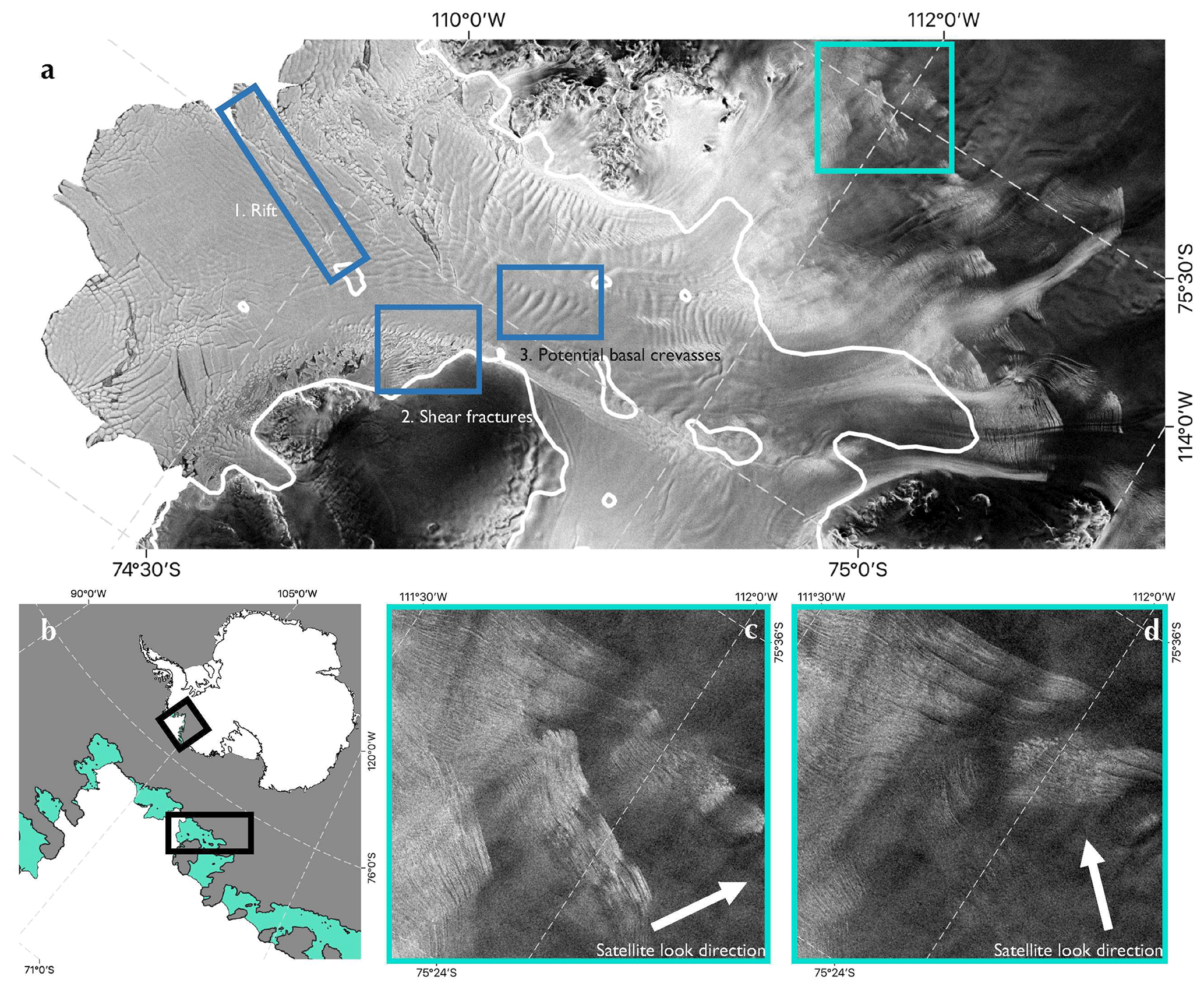
Figure 1Crevasses visible in SAR data covering Crosson Ice Shelf, West Antarctica. A Sentinel-1 SAR image acquired on 1 June 2021 covering Crosson Ice Shelf is shown in panel (a). Blue boxes show examples of type-A crevasses on the floating ice: 1: rift; 2: shear fractures; 3: smooth depressions potentially resulting from basal crevasses. The green box shows type-B crevasses on grounded ice shown larger in panel (c). The white line shows the MEaSUREs grounding line (Rignot et al., 2016). Panel (b) shows the location of the Crosson Ice Shelf region within the Amundsen Sea Embayment (ASE) and, in turn, the location of the ASE within Antarctica. Grey represents grounded ice and green represents floating ice – according to the MEaSUREs grounding line. Panel (c) shows a blown-up part of the large SAR image shown in panel (a) covering a patch of heavily crevassed grounded ice. Panel (d) shows this same patch for a SAR image taken on the same day at a near-perpendicular angle to that shown in panel (c). The satellite look angles are shown in panels (c) and (d) by the white arrows. The visibility of type-B features changes dramatically between the images taken at different acquisition angles.
2.1 Methods
Brittle fracture occurs mechanically in three modes, which are commonly denoted as I, II and III (Irwin, 1957). Mode I represents cracks opening in the direction of the applied tensile stress, while modes II and III represent cracks caused by in-plane and out-of-plane shear stresses respectively (Benn and Evans, 2014; Colgan et al., 2016). Additionally, due to the viscoplastic properties of ice, ductile processes can augment these brittle failure modes and produce complicated crevasse patterns. Mode-I failure tends to result in parallel, sharp-sided surface crevasses or rifts clearly visible in the Sentinel-1 backscatter signal and basal crevasses which can result in visible large-scale depressions in the surface (Vaughan et al., 2012; Luckman et al., 2012; McGrath et al., 2012), especially if subject to subsequent ductile deformation (“necking”) above the crack tip (Bassis and Ma, 2015). However, it is difficult to discern whether such depressions are an indicator of basal crevasses or other processes such as channelised melting of the sub-shelf, so we focus our methods on the detection of surface crevasses in the knowledge that the sharpest-looking basal crevasses (i.e. where there are large-magnitude intensity gradients perpendicular to the crevasse walls) will be detected as well. Shear failure, ubiquitous in the margins of fast-flowing ice streams and shelves, can result in macroscopic crevasses or rifts when severe. Often, however, it results in interacting networks of microfractures, particularly on grounded ice streams. Though regions of high backscatter can indicate that the ice is rougher in the shear margins than elsewhere on the glacier, the “micro” nature of these fractures means that we cannot rely on seeing them in the surface signal, so we do not attempt to map this type of diffuse fracture.
In general, we restrict our attention to “sharp-sided” features that appear crevasse-like in isolation: largely surface fractures from mode-I and shear failure. We classify these features into two sets: type-A and type-B, based on their qualitatively different expressions in the backscatter data (Fig. 1). Different methods are required for the extraction of these different classes given the disparity in their visual appearance, and the resulting datasets are useful for different purposes. Type-A features are large, multiple pixels in width, and are visible from many look angles of the satellite. Type-B features appear as fine, bright lines in the backscatter images. They can be pixel scale in width and are most visible when the horizontal component of the satellite acquisition angle is perpendicular to the crevasse walls. Hence, these features need to be recovered from data covering multiple acquisition angles. Happily, in many places, the Sentinel-1 acquisition tracks overlap obliquely and, often, at near-perpendicular angles (Fig. 1c and d). Broadly, these two categories distinguish crevasses on floating and grounded ice: type-A features include ice shelf surface crevasses, rifts and any basal crevasses that cause narrow surface depressions, while type-B features include grounded surface crevasses and, to a far lesser extent, narrow ice shelf surface crevasses bridged by snow.
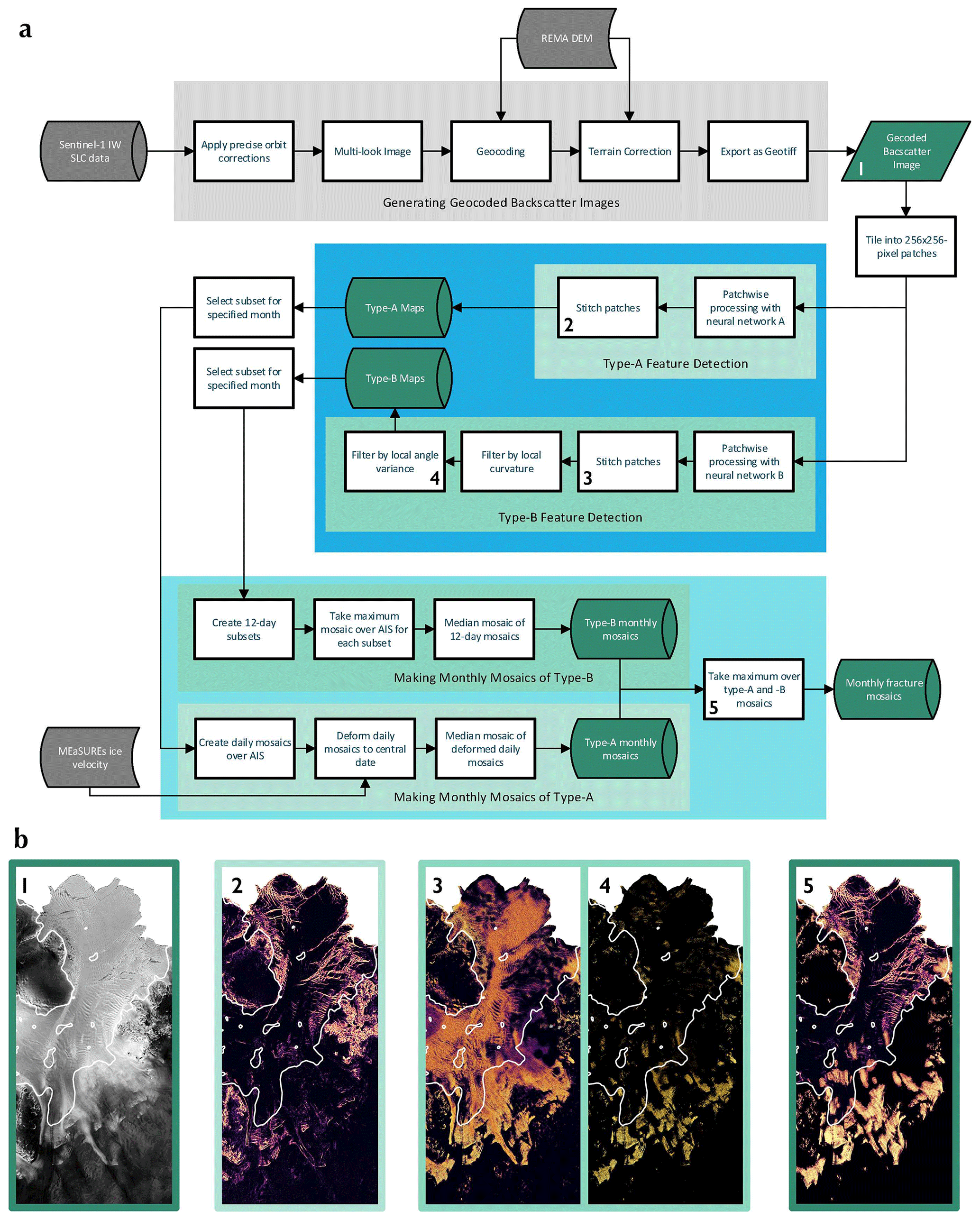
Figure 2Outline of the processing chain that takes a month of Sentinel-1 IW SLC data and produces a fracture mosaic. Panel (a) shows a flow diagram representing the process. Panels (b1–5) show different stages of processing for an example SAR image over Crosson Ice Shelf. In each panel (b2–5), features that appear brighter are more likely to be crevasses according to the latest processing step. Numbers in the top-left corner correspond to the stages of processing that match the numbers in the flow diagram (a). (b1) A 50 m resolution SAR backscatter image from 1 June 2021. (b2) The image after processing with the neural network NA, showing type-A features. (b3) The image after processing with the neural network NB. This displays type-B features along with considerable noise on the floating ice. (b4) The result of applying the type-B filtering algorithm to panel (b3). Most of the noise is seen to be removed, leaving type-B features visible from that particular look angle. (b5) A mosaic for the month of June 2021 from images like those displayed in panels (b2) and (b4). The superimposed white lines show the MEaSUREs grounding line (Rignot et al., 2016).
We developed two neural networks and additional filtering techniques to identify these separate features from individual geocoded single-look complex (SLC) amplitude images, acquired using the interferometric wide-swath (IW) mode of Sentinel-1 and methods for constructing combined monthly mosaics of type-A and type-B crevasses. Figure 1 shows example type-A and type-B crevasses visible in Sentinel-1 SAR data over Crosson Ice Shelf. Figure 2 shows an overview of the procedures involved in constructing monthly fracture mosaics, such as that shown in Fig. 4.
2.1.1 Bootstrapping neural networks
The networks used for the extraction of type-A and type-B crevasses share a similar architecture but were trained separately, resulting in networks we call NA and NB. The network architectures are essentially U-Net (Ronneberger et al., 2015), similar to those used in Lai et al. (2020) and Zhao et al. (2022), though shallower and lower-dimensional. This is because many of the features we are interested in, such as type-B crevasse fields and rifting in ice shelf shear margins, are textural in nature. In order to avoid the laborious process of creating a training dataset by the manual annotation of satellite images, we employed a bootstrapping technique of the same kind detailed in Surawy-Stepney et al. (2023). In short, we initially trained the networks on a small training dataset consisting of pairs of SAR backscatter images and manually annotated calving front positions, the same as those used to train the calving front network in Surawy-Stepney et al. (2023) (Fig. 3a). Training was stopped considerably before convergence of the network parameters, resulting in networks capable of removing speckle from SAR images and highlighting semantic edges. The intuition behind this is that calving fronts represent a subset of linear, textural discontinuities in the SAR images which is ultimately defined by larger-scale contextual or semantic information. Early on in training, due to the hierarchical nature of U-Net, along with its skip connections, the cost function can be reduced quickly using activations from the shallower layers which correspond to low-level textural information such as the presence of spatial intensity gradients, i.e. edges, at the pixel level. The deeper layers might contribute semantic information on the length of linear features, though not that which differentiates the calving front edge from crevasse walls.
We then applied these partially trained networks to unseen data and manually selected images for which the network assigned relatively large values to the locations of crevasses (Fig. 3b and c). A scaling was applied to these outputs to enhance the crevasse features, and the scaled outputs were added along with the corresponding input image to an updated training dataset (for either type-A or type-B). We then retrained the networks on these larger datasets. This constitutes one round of a “bootstrapping” procedure that, after three to four iterations, led to a training dataset of ∼103 256×256-pixel, 64-bit images and networks that perform well in the desired task. Each time the networks were trained, their parameters were initialised to the values at the end of the last round of training. Hence, scaling the output images before adding them to the new training datasets was necessary to induce non-zero gradients of the cost function with respect to the network parameters.
By separately applying the networks NA and NB to input SAR images, we create type-A and intermediate type-B crevasse maps for each Sentinel-1 acquisition frame individually. To do this, SAR images are tiled into 256×256-pixel patches, overlapping by half, processed by the neural networks NA and NB respectively and pieced together. For each network, a softmax function is applied to the output, and the channel corresponding to “crevasse” is selected so that the outputs are normalised to the range [0,1] for each pixel, where 1 represents a high confidence of a crevasse and 0 a low confidence.
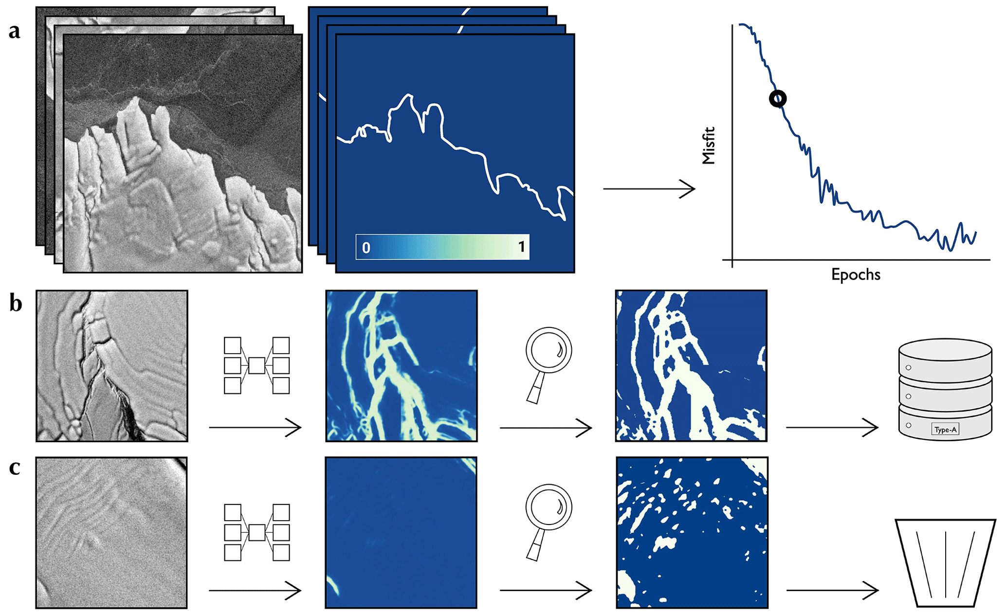
Figure 3Bootstrapping partially trained neural network NA. (a) Example input–target pairs for the initial phase of training of the randomly initialised network. Training was stopped well before parameter convergence. (b, c) Bootstrapping. The network was applied to unseen images and the outputs were visually inspected. If the outputs could be thresholded to look like a plausible target image (b), that threshold was applied before the input–output pair was added to a new training dataset. If not (c), that input–output pair was discarded.
2.1.2 Type-A
We directly use the outputs from the neural network NA as our map of type-A crevasses. If required, a threshold can be applied to produce binary maps, with optimal values that depend on the features of interest and the desired balance between performance metrics.
2.1.3 Type-B
The outputs of the neural network NB highlight many of the fractures visible in the input images but often contain spurious collections of randomly aligned features (Fig. 2b3). Visual assessment of the SAR backscatter images shows type-B crevasses to be linear on kilometre scales and exists in patches of crevasses that are locally parallel. We have developed a filtering algorithm that we call “parallel-structure filtering” (PSF), which we apply to the network outputs to remove features that fail to conform to these conditions (Fig. 2b4). This starts by calculating the Hessian matrix local to each data point using Gaussian derivatives. The likelihood of each pixel being part of a linear structure is subsequently calculated from the Hessian eigenvalues (Frangi et al., 1998; Jerman et al., 2016), and those with a likelihood above a certain threshold are kept. The angles of the structure on which these data points lie are extracted from the Hessian eigenvectors before a local distribution of angles is calculated with a set of box-kernel convolutions. Data points are removed if the local angle variance exceeds a threshold of 0.71 tuned to best fit a small set of example manual annotations. Further details on the algorithm are provided in Appendix A.
2.1.4 Making monthly mosaics
The methods described above allow us to produce separate type-A and type-B crevasse maps for individual Sentinel-1 acquisition frames. We create individual, pan-continental type-A and type-B crevasse maps each month by combining these individual frames before stitching these together to create combined type-A and type-B mosaics. For type-A features, we make the approximation that crevasses move and deform according to the surface ice velocity and compensate for this with a Lagrangian correction in which we post the maps to a common date at the middle of the time period using a remapping defined by the MEaSUREs Antarctic ice velocity dataset (Mouginot et al., 2012; Rignot et al., 2017). We then take a simple median mosaic over the time window of choice.
As mentioned above, type-B mosaics are complicated by the fact that the visibility of the features is dependent on the look angle of the satellite. Hence, before taking a median mosaic, we break the time period into 12 d windows that capture all look angles of the satellite and take maximum mosaics over each. We do not provide a Lagrangian correction for the type-B mosaics, because their visibility often does not persist as they are advected downstream, and the locations where they are produced do not appear to change on monthly timescales. The final crevasse map is produced by masking the grounded ice sheet areas in the type-A mosaics before taking a maximum composite with the type-B fracture mosaic. This results in a normalised score , with 1 indicating “fracture” and 0 indicating “no-fracture” for each pixel on the map. We note that we are unable to map the fractures on large parts of the Ronne–Filchner and Ross ice shelves and much of the interior of the Antarctic Ice Sheet, due to the latitudinal limits of the Sentinel-1 data acquisition plan.
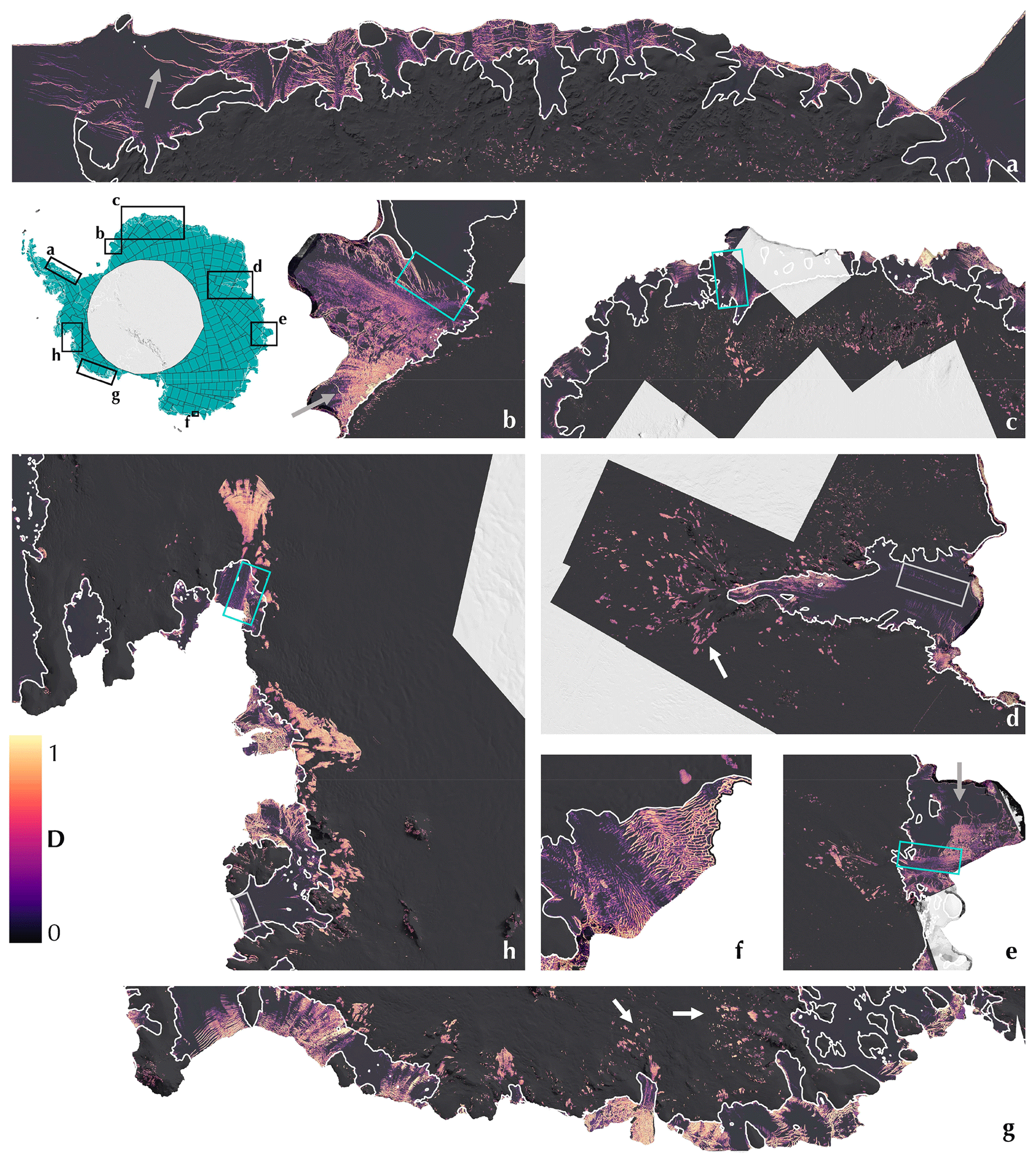
Figure 4Fractures in Antarctica: April 2022. Results at different scales from a pan-continental fracture mosaic. is a normalised score with 1 indicating “fracture” and 0 indicating “no-fracture” for each pixel. The labelling of sub-figures corresponds to a clockwise ordering around the Antarctic coastline starting from the Eastern Antarctic Peninsula. (a) The Larsen D Ice Shelf. (b) The Brunt–Stancomb–Wills Ice Shelf. (c) Dronning Maud Land including Fimbul Glacier and Fimbul Ice Shelf. (d) Amery Ice Shelf and its basin – including Lambert Glacier. (e) Shackleton Ice Shelf and Denman Glacier. (f) Cook Ice Shelf. (g) The coastline between the West Getz (left) and Salzburger (right) ice shelves, with the land ice tongue in the centre. (h) The Amundsen Sea Embayment, including, from top to bottom, Pine Island Glacier, Thwaites Glacier, Crosson Ice Shelf and its tributary glaciers, and Dotson Ice Shelf. Boxes and arrows overlaying the enlarged parts of the crevasse map highlight features mentioned in the main text: blue boxes show fractures in ice shelf shear margins, grey boxes show where crevasses that are known to exist appear only faintly in the crevasse map, white arrows show type-B fractures, and grey arrows show large rifts. The top-left inset shows the Antarctic Ice Sheet with the locations of images (a)–(h) identified with black boxes. These give a sense of the different scales at which crevasses can be seen. In teal, we show the total extent of all Sentinel-1 acquisitions over the AIS so far. The white line shows the MEaSUREs grounding line (Rignot et al., 2016).
2.2 Results
We applied the method described above to every Sentinel-1 acquisition between January 2015 and July 2022 and produced composite crevasse maps covering the Antarctic Ice Sheet for each month. Figure 4 shows an example map made using Sentinel-1 acquisitions from April 2022. The results show crevasses to be a feature of a large and varied set of ice streams and shelves across the continent – from rifts in the shear margins of the fast-moving ice shelves of the Amundsen Sea (Fig. 4h) to the fine surface fractures fringing the grounded ice streams of the Amery Basin (Fig. 4d).
The type-A fractures identified by the network take a wide variety of forms and are exclusive to floating ice shelves. Of those observed, the brightest and most identifiable are large ice shelf rifts, such as Chasm-1 on Brunt Ice Shelf and those penetrating into the bulk of Shackleton and Larsen D ice shelves (highlighted with grey arrows in Fig. 4b, e, a respectively). Many fast-flowing ice shelves exhibit severe crevassing in shear margins that connect them to slower-flowing parts of the ice shelf, for example on Stancomb–Wills Ice Tongue, Fimbul Ice Shelf, Shackleton Ice Shelf and Pine Island Ice Shelf (highlighted with blue boxes in Fig. 4b, c, e, h respectively). We also see fractures resulting from the interaction of ice shelves and ice rises around the coastline – for example on Larsen D Ice Shelf (Fig. 4a).
Our observations show that type-B crevasses, though a less varied set of features, are as prevalent across the continent as type-A crevasses and occur in every major basin of the Antarctic Ice Sheet, generally in dense patches. Approximately 85 % of type-B crevassing appears on grounded ice. Our observations show that type-B crevasses are particularly dense and widespread in the ice streams of the Amundsen Sea Embayment (Fig. 4h). In a composite crevasse map of the grounded part of the ice sheet from June 2021, this region accounted for around 10 % of grounded crevasses despite covering only 3.5 % of the imaged surface area. These ice streams have undergone significant dynamic change over the last few decades, with ice flux across the grounding line increasing by 40 % to 100 % since the early 1990s (Shepherd et al., 2004; Mouginot et al., 2014; Joughin et al., 2014; Konrad et al., 2017; Davison et al., 2023). The large number of grounded crevasses observed in this region may be a consequence of the sudden increase in longitudinal strain rates which will accompany the observed speedup. The effect of crevasse fields like this could be to decrease the effective viscosity of the ice. Hence, fracturing can provide a mechanism for the sudden manifestation and persistence of ice dynamic changes, beyond that which can be accounted for by dynamic thinning. In many grounded areas, however, crevasse depth is likely to be only a small fraction of ice thickness due to large overburden pressures (Benn and Evans, 2014).
Elsewhere around Antarctica, surface crevasses on grounded ice appear sporadically in patches. In some instances, they contour the edges of ice streams, such as on Lambert Glacier in East Antarctica (white arrow, Fig. 4d). Elsewhere, the locations of patches of crevasses appear dependent on vertical shear stresses, for example mode-I crevasses forming due to abrupt changes in basal slip or mixed-mode crevasses caused by sharp changes in bed topography (white arrows, Fig. 4g). The sizes of these patches of crevassed ice are of the order of ∼10–100 km in the along-flow direction, showing that the crevasses can be healed when stress conditions change. Crevasse visibility is also influenced by spatial variability in the depth of drifting snow and, in regions for which image acquisition angles vary little, changing crevasse orientation. In future, we can hope to constrain these additional factors using additional sensors to better bound the regions in which type-B crevasses appear on grounded ice.
We finally note that, due to the shallow networks, the bootstrapping procedure, and the absence of training data seaward of the Antarctic coastline, the networks are sensitive to local textural deviations at, and beyond, the calving front. For example, leads and fractures in sea ice, dense ice mélange, iceberg boundaries and calving fronts exhibit strong signals in the fracture mosaics when unmasked.
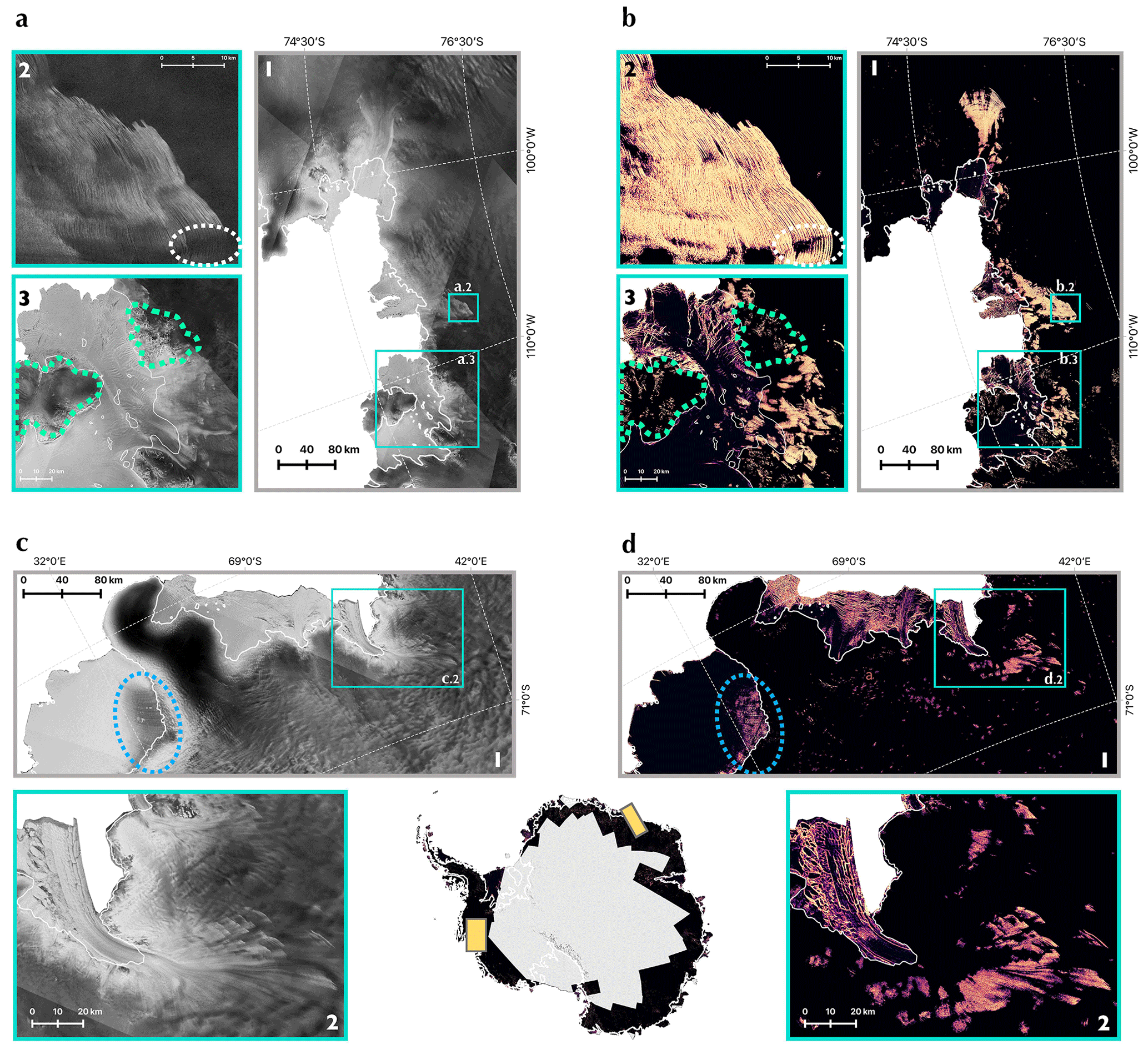
Figure 5A comparison between a composite SAR image and crevasse map (June 2021). The left-hand side of the figure shows parts of the SAR backscatter composite (a simple mosaic, with later frames overlaying earlier ones), while the right-hand side shows the corresponding parts of the fracture map. (a) SAR images covering the Amundsen Sea Embayment: (a1) the glaciers of the ASE and the locations of the enlarged regions (a2) and (a3) shown as cyan boxes, (a2) enlarged region over the grounded crevasses fringing the Thwaites Glacier ice stream, and (a3) enlarged region over Crosson Ice Shelf and the surrounding glaciers. Panels (b1)–(b3) show the corresponding crevasse maps. White dashed ovals show where crevasses are not visible in the SAR image or the crevasse map despite likely connecting crevasses either side. Green dashed boundaries show regions of steep topography on Bear Island and Mount Murphy, where type-B crevasses appear erroneously in the fracture map. (c) SAR images over a part of eastern Dronning Maud Land. (c1) The region as a whole and the location of the enlarged region (c2) shown as a cyan box. (c2) Enlarged region over Shirase Glacier and Shirase Ice Shelf. Panels (d1)–(d2) show corresponding crevasse maps. Blue dashed ovals show the location of surface meltwater on Baudouin Ice Shelf, where crevasses appear erroneously in the fracture maps. Panels (b) and (d) inherit the colour map from Fig. 4. In each figure, the white line shows the MEaSUREs grounding line (Rignot et al., 2016). The bottom middle shows a map of Antarctica with the full June 2021 crevasse map overlaid on the MODIS map of Antarctica (Haran et al., 2021); yellow boxes show the boundaries of the locations of the parts shown in panels (b1) and (d1).
2.3 Evaluation
Overall, we consider the Antarctic fracture maps we produce to be an accurate representation of crevasses across the continent that are linear on scales that are large compared to the resolution of the data, with a few exceptions. There are two components that inform this conclusion. Firstly, previous studies suggest that the majority of such crevasses are visible as type-A or type-B features in the Sentinel-1 SAR backscatter images (Moctezuma-Flores and Parmiggiani, 2016; Thompson et al., 2020; Marsh et al., 2021). Secondly, the methods we have developed extract a majority of features in the backscatter images while highlighting a few features erroneously. The fracture maps covering Dronning Maud Land, the Amundsen Sea sector and the eastern Antarctic Peninsula (Fig. 4b, g and h respectively) show the lack of noise present in the monthly mosaics at different scales – indicating a high specificity for both type-A and type-B crevasses. In large part this can be attributed to the ability of the neural networks to deal with radar speckle and the efficacy of our parallel-structure filtering algorithm. These figures also show how mosaicking over monthly windows results in maps that do not display visible processing artefacts, such as the edges of SAR frames or boundaries between regions of different acquisition geometry. In part this is a consequence of using raw, un-normalised SAR data. This provides confidence that large features can be mapped across image acquisition boundaries and therefore provides a good representation of the ice sheet surface.
The few locations in which type-B features are present in the crevasse maps without obvious fractures visible in the backscatter images are in regions of steep topography, such as the ice rises and mountains around Crosson Ice Shelf (Fig. 5a3, b3, circled in green). As the topography of these regions is essentially unchanging over the time period of this study, these features could be dealt with by defining a mask based on the gradients of a digital elevation model or by retraining the neural networks with additional data covering such areas of steep terrain. However, as these regions are distinct from those with the kind of large-scale dynamic behaviour we are interested in, the misattribution of crevasses to these areas is incidental.
The specificity of crevasse detection is also low in regions where there is a large amount of surface meltwater – for example near the grounding line on Roi Baudouin Ice Shelf in eastern Dronning Maud Land (Fig. 5c1, d1, circled in blue). Values of type-A crevasse probability are high in regions of surface melt due to the presence of features that are not usually visible, such as sharp contrasts in backscatter at the boundaries of melt ponds, fluvial features originating from the persistent pooling and flow of surface water (e.g. near the grounding line of Amery Ice Shelf – Fig. 4c) as well as a greater sharpness of shallow surface depressions due to the decrease in microwave penetration depth. In static crevasse maps such regions appear to have a greater amount of crevassing compared to nearby areas with a comparable surface structure. However, there are only a few locations for which this is a persistent issue (e.g. Amery and George VI ice shelves), with other locations only experiencing melt events in the austral summer (e.g. eastern Dronning Maud Land). However, the effect of meltwater, even if intermittent, means caution is required when comparing crevasse maps covering ice shelves known to be affected by surface meltwater at different locations or times. If surface melt in Antarctica increases in the future in response to a changing climate, then methods will need to be developed to remove these features – or conversely to isolate and use the information as a proxy dataset for meltwater extent.
The method appears sensitive to the great majority of crevasse-like features visible in the backscatter images across the continent. Unsurprisingly, it is most sensitive to sharp-sided ice shelf surface crevasses and rifts. However, some smooth features – likely to be basal crevasses – are under-represented in the type-A maps, for example those near the calving front of Dotson Ice Shelf and those forming a track along the central–western part of Amery Ice Shelf (shown by grey boxes in Fig. 4h and d respectively), which appear only faintly.
The type-B mapping identifies the bulk of crevasses visible in the images. The exception is at the boundary of patches of grounded crevassing where the edges are sometimes cut off by the low-resolution filtering. There are also crevasse fields that include small regions, of the order of 5 to 10 km in width, in which crevasses likely exist but are less visible in the backscatter images (e.g. on the Thwaites ice stream – Fig. 5a2, b2, circled in white). These regions are blank in the crevasse maps, despite the fact that crevasses very likely propagate through them, linking the identified crevasses on either side.
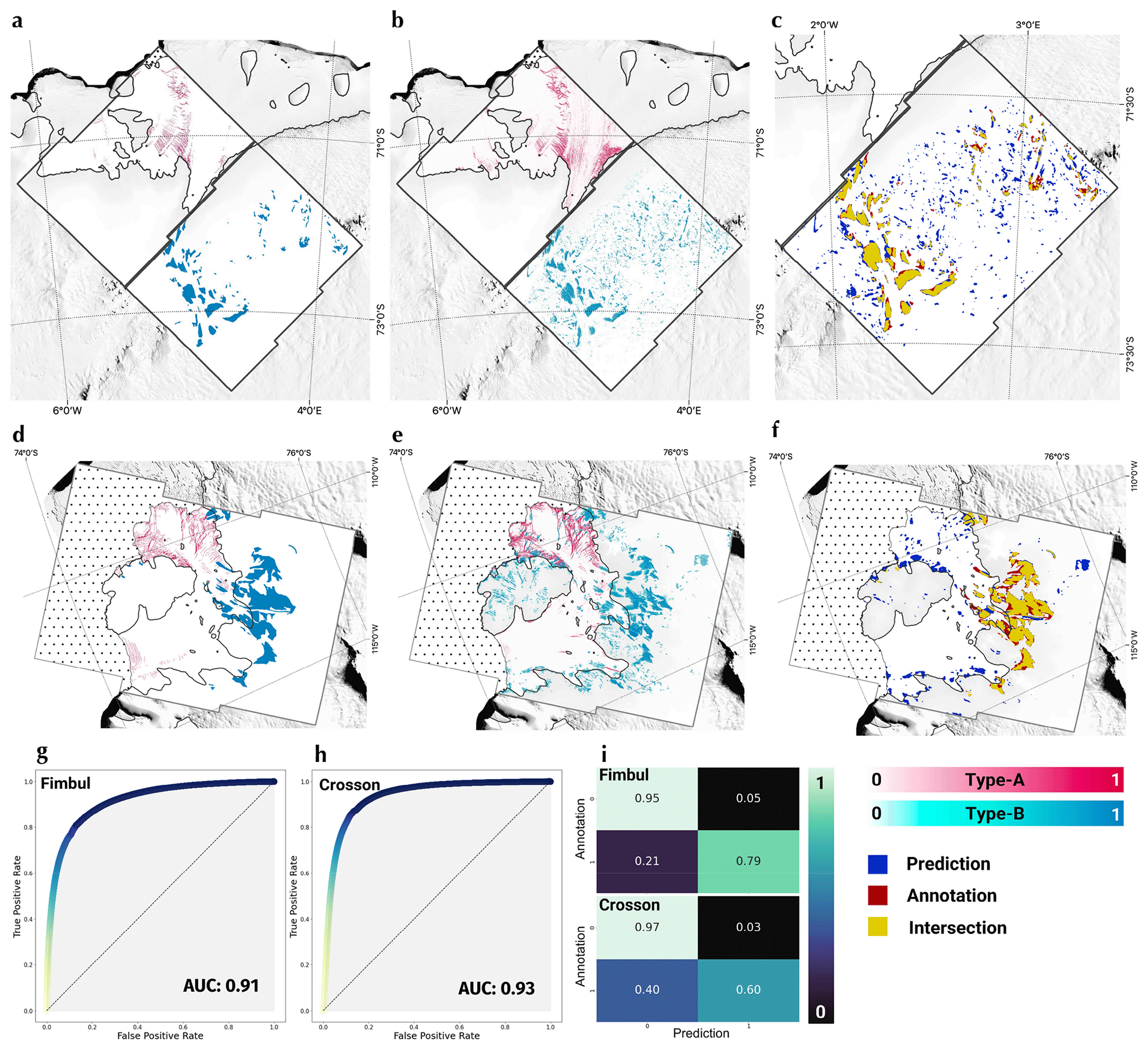
Figure 6Evaluation of type-A and type-B crevasse maps against manual annotations for Sentinel-1 frames covering Crosson and Fimbul ice shelves and their tributary ice streams. (a) Annotated type-A crevasses and type-B crevasse fields covering two Sentinel-1 SAR frames over Fimbul Glacier (PFs 2/931 and 2/925, dated 15 August 2018). (b) Corresponding monthly mosaic of type-A and type-B features over SAR frames PFs 2/931 and 2/925. (c) The intersection of the type-B field annotations and the smoothed and thresholded type-B mosaic for PF 2/925. (d) Annotated type-A (red) crevasses and type-B crevasse fields for a Sentinel-1 SAR frame covering Crosson Ice Shelf and its tributaries (PF 7/913, dated 7 June 2021). (e) Corresponding monthly mosaic of type-A and type-B features for PF 7/913. (f) The intersection of the type-B field annotations and the smoothed and thresholded type-B mosaic for SAR frame PF 7/913. (g) ROC plot for type-A features for Sentinel-1 PF 7/913 (labelled “Fimbul”). (h) ROC plot for type-A features for Sentinel-1 PF 7/913 (labelled “Crosson”). (i) Confusion matrices for type-B field annotations and the smoothed and thresholded type-B mosaic for Sentinel-1 PFs 2/925 (labelled “Fimbul”) and 7/913 (labelled “Crosson”). The background on which the SAR frames are overlaid is the MODIS MOA (Haran et al., 2021; Greene et al., 2017). The grounded ice within the SAR frames is shaded using the REMA 1 km DEM (Porter et al., 2018). The grounding line shown is according to MEaSUREs (Rignot et al., 2016) (black line). The spotted regions indicate the sea.
To further assess the performance of our type-A and type-B fracture maps and to quantify statements regarding the specificity and sensitivity of our crevasse maps, we compared the monthly mosaics with three manually annotated Sentinel-1 IW SAR frames, created independently, without reference to the fracture mosaics. The European Space Agency provides in-house references for the relative orbit and frame numbers for the image acquisitions which we shall use to distinguish the SAR images here and in the rest of the article. We will refer to the relative orbit number as “path” and abbreviate the path and frame that identifies a specific acquisition as “PF”. The three SAR images chosen cover Crosson and Dotson ice shelves and their tributary glaciers (PF 7/913, dated 7 June 2021), Fimbul Ice Shelf (PF 2/931, dated 15 August 2018) and the grounded Fimbul Glacier (PF 2/925, dated 15 August 2018). We annotated these in their entirety in order to help facilitate future intercomparison with other methods. We selected these frames to represent a challenge to the method, as the full variety of crevasse features is present together with large regions of steep topography and persistent surface melt. For type-A features, we annotated individual crevasses at the pixel level in single SAR images corresponding to the chosen frame. However, for type-B features, it is all but impossible to pick out individual crevasses by hand. Instead, we delineated the boundaries of crevasse fields, which we then compared with versions of the type-B mosaics that were smoothed and thresholded to produce binary maps of contiguous crevasse fields. For the case of the SAR image covering Crosson Ice Shelf, we combined annotations from the given frame and another with a relatively oblique acquisition angle (PF 10/855, dated 7 June 2021) to reflect the different crevasses that were visible from the different angles. Given the continuous output and class imbalance inherent in the type-A mosaics, we produced receiver–operator characteristic (ROC) curves for the evaluation of the type-A maps, while we report confusion matrices for the evaluation of the type-B processing. Results are shown in Fig. 6.
The ROC curves quantify the sensitivity or specificity of the type-A mosaics over the full range of threshold values [0,1]. The areas under the curves for the frames covering Crosson, Dotson and Fimbul ice shelves respectively are 0.93 and 0.91, showing high discriminatory power (Fig. 6g and h). This is despite the failure of the network to extract a large portion of the likely basal crevasse impressions on Dotson Ice Shelf (Fig. 6d and e), those west of the Fimbul western shear margin (Fig. 6a and b), and the misattribution of flow features on the central trunk of Fimbul Shelf and fluvial features in its eastern shear margin as crevasses (Fig. 6a and b). The intersections of the annotated and predicted crevasse fields show a great deal of overlap in the crevasse fields on Fimbul (Fig. 6c), Pope, Smith and Kohler (Fig. 6f) glaciers, with the largest fields sharing the most overlap. There are a number of smaller features in the type-B mosaics that do not appear in the annotations – especially in the case of Fimbul Glacier and surroundings. This is where mountains and steep rocky features have been identified by the model as crevasses. However, the confusion matrices (Fig. 6i) show that these areas cover under 5 % of the total “undamaged” ice according to the manual annotations.
3.1 Methods
After establishing the above method of reliably extracting fracture-location data, we moved onto the natural question of whether it is possible to use this dataset to measure changes to “damage” through time. At the outset it was unclear whether the 7.5-year study period was long enough for real structural change to evolve in response to ice dynamic processes in Antarctica or whether the impact of radar interactions with the ice surface properties may cause crevasse mapping to vary too much in response to environmental factors unrelated to crevasse evolution, such as weather-induced surface melt. It is certainly clear that variability in the properties of the ice surface renders the direct comparison of fracture maps at different times an unreliable method of assessing change.
The method we introduce here measures trends in the local density of fractures using the full time series of fracture maps, producing a scalar “fracture density change” value that can be used to compare different locations.
A brief analysis of the fracture maps shows minor changes to crevassing on the grounded ice sheet over the last 7.5 years. We therefore focused on ice shelves, where crevasse patterns change on shorter timescales due to elevated flow speeds, interaction with rapidly changing ocean conditions and higher-amplitude loading–unloading cycles. More specifically, we considered the ice shelves of the Amundsen Sea Embayment, given that a large amount of the ice dynamic change in Antarctica was observed in that region between 2015 and 2022.
We define fracture density as the fracture maps integrated over an area of interest (Albrecht and Levermann, 2012; Surawy-Stepney et al., 2023) and use this as a heuristic measure of how crevassed that region is. We looked for linear trends in this parameter over the observational period. To analyse the spatial pattern of change, we first defined a fixed 2.5 km×2.5 km grid of points over the ice shelves. Time series of fracture density and backscatter standard deviation were extracted from daily mosaics over a 10 km×10 km square buffer around each point before the fracture density change and error were found. Given that we were not interested in the development of individual crevasses, we did not apply Lagrangian corrections to the crevasse maps.
As mentioned above, we had to account for the dependency of our fracture maps on the surface properties of the ice before calculating trends in the time series. For example, seasonal changes to crevasse visibility due to changing firn water content or thickness of the snowpack can dominate the signal over changes in crevasse length or concentration (Marsh et al., 2021). It was necessary, therefore, to separate the parts of the signal due to real changes in the crevasse pattern and those due to changes in the surface expression of the crevasses resulting from such unknown environmental factors. This is only possible given the large number of crevasse maps, and hence fracture density data points, in the time series given the short repeat period of the Sentinel-1 satellites. Firstly, we discarded measurements made between December and March each year, due to the prevalence of surface melt during those months. We then made use of the observation that the surface properties of the ice seem to be discernible from the local standard deviation of the backscatter signal. We used this as a proxy to define sets of dates for which ice surface conditions were similar and constructed an ensemble of fracture density time series for each region. By taking a weighted mean and standard deviation of the trends and multiplying by the time span, we defined an estimated fracture density change over the time period (Fig. 7a, b, f, j) and provided an uncertainty (Fig. 7c, j, k). See Appendix B for more details.
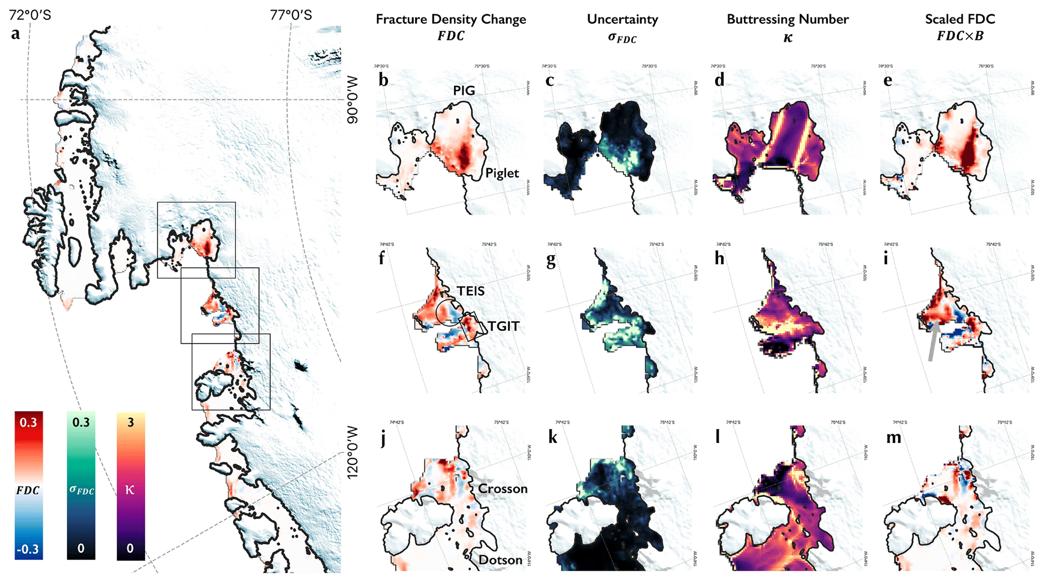
Figure 7Structural change in the ice shelves of the ASE. (a) An overview showing the change in fracture density from January 2015 to July 2022 for the ASE as a whole. Grounded ice, according to the MEaSUREs grounding line (Rignot et al., 2016), is represented with the REMA 2 km DEM (Porter et al., 2018). The table of panels (b)–(m) shows expanded maps of fracture density change (b, f, j), uncertainty in fracture density change (c, g, k), buttressing number (d, h, i) and fracture density change scaled by buttressing number (e, i, m) for Pine Island (b–e), Thwaites (f–i) and Crosson (j–m) ice shelves.
3.2 Results
By applying the method defined above to daily fracture map mosaics, we derived an estimated change in fracture density for the ice shelves of the ASE (Fig. 7a). For the most part, our results show that notable changes in fracture density over the observational period were confined to Pine Island, Thwaites and Crosson ice shelves (Fig. 7b, f, j respectively), with change elsewhere attributable to modest calving events or terminus advance (Fig. 7a).
On Pine Island (Fig. 7b–e), a large region of fracture density change in the interval 0.08–0.3 shows a significant deterioration of the southern shear margin over the observational period (Lhermitte et al., 2020), continuing a decades-long pattern of structural decline on this ice shelf (MacGregor et al., 2012). The intense fracture density change at the seaward-most part of the shear margin reflects its disintegration over the course of 2020 (Figs. 7b, 8b and c), completely decoupling the ice shelves of Pine Island Glacier and Piglet Glacier which, until 2018, flowed north-east into the southern shear margin of Pine Island Ice Shelf, rendering it unbuttressed and marine-terminating. We also see a general region of increased fracture density at the seaward limit of the ice shelf, which can be attributed to a series of propagating rifts forming downstream of an ephemeral grounding point near the centre of the ice shelf that led to calving events between 2015 and 2020 (Joughin et al., 2021).
Moving around the coast of West Antarctica to the ice shelves of Thwaites Glacier (Fig. 7f–i), a more complicated picture emerges. On the Eastern Ice Shelf, the data suggest a highly variable pattern of structural change. A patch of decreasing fracture density (black circle, Fig. 7f) indicates where sharp-sided crevasses have travelled further onto the shelf, followed by smoother (likely shallower-surface or basal) crevasses (Fig. 8d). Around the pinning point to the north of the ice shelf, we see decreased fracturing around its western end and increased fracturing to the south and east. This is due to crevasses or rifts opening up in situ, perpendicular to the orientation of the pinning point on the main body of the shelf in response to increased shear stress in the latter half of the 2010s (Benn et al., 2022).
Thwaites Glacier's western ice tongue displays increased fracture density on the floating section of the main trunk closest to the grounding line and in the ice to the south of the eastern shear margin (black box, Fig. 7f). Fracturing on the central trunk has been increasing steadily over the observational period, while that on the eastern shear margin increases and decreases with acceleration of the main trunk (Surawy-Stepney et al., 2023). Changes to fracturing in the regions closest to the grounding line have been periodic on timescales of a few years (Fig. 8b and d), so our linear trends do not capture the behaviour of this region in full. The protruding ice tongue has been degrading steadily over the observational period (Miles et al., 2020; Surawy-Stepney et al., 2023). However, while our data show a large region of positive change in fracture density, negative trends in fracture density are shown on the eastern side of the ice tongue. This reflects a reduction in the density of the mélange separating the ice tongue from the Eastern Ice Shelf, where, at some point, our fracture maps stop recognising the spaces between icebergs as fractures.
Our observations show changes in fracture density on the main body of Crosson Ice Shelf and in its shear margins (Fig. 7j–m). On the main body, these are largely due to the advection of rifts towards the ocean, as can be seen by the stripes of increasing and decreasing fracture density (Fig. 7j), though fracturing has progressed and increased slightly in density on the shear margins. Finally, we note that, despite our observations showing fracture density change outside of the Amundsen Sea sector to be limited (Figs. 7a, 8b), some ice shelf crevasses which may be linked to interesting glacial processes – such as those perpendicular to the direction of ice flow that follow the sub-shelf melt channel in the western part of Dotson Ice Shelf (Gourmelen et al., 2017) – are not visible in our fracture maps (Figs. 4h, 8f). This is because they have a distinctive visual representation in comparison to type-A and type-B crevasses, which the two neural networks used in this study are not tuned to detect. Future studies should seek to evolve the existing method to identify and map additional classes of crevasses across Antarctica, which will be a useful dataset for assessing different glaciological conditions.
After measuring the spatial pattern of fracture density change in the Amundsen Sea sector, we investigated where these changes might be important for the dynamics of the glaciers. To evaluate how changes to the local stress distribution might impact the glacier at large, we employed the fractional difference between the second principal component of the vertically integrated viscous stress tensor e2 and the vertically integrated hydrostatic pressure as a local notion of “buttressing” (Gudmundsson, 2013; Fürst et al., 2016); Appendix C:
where , ρi is the density of ice, ρw is the density of sea water, g is the acceleration due to gravity and h is the ice thickness.
By weighting the fracture density change by this buttressing number as it was at the start of the observational period, we assessed where observed changes to fracturing might have a meaningful impact on the ice dynamics (Fig. 7e, i, m). For example, where a major increase or decrease in fracture density had occurred in a buttressing region of an ice shelf, we expect to also observe a dynamic change. Our observations show that the large increase in fracturing in the southern shear margin occurred in a strongly buttressing part of the ice shelf (Fig. 7e). Similarly, those changes to crevassing on the Thwaites Eastern Ice Shelf are amplified around the offshore pinning point when buttressing is taken into consideration, while changes on the main body of Crosson Ice Shelf are diminished.
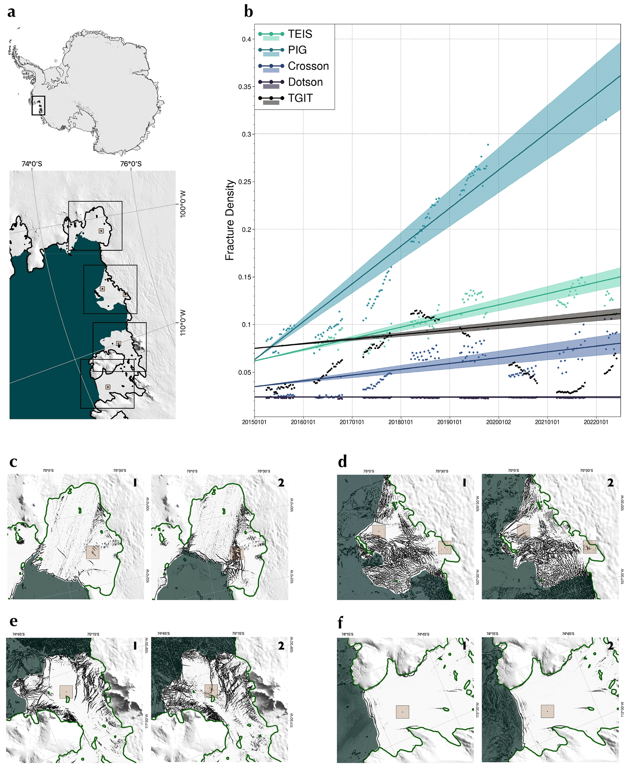
Figure 8Time series of fracture density at specified points on the ice shelves of the Amundsen Sea Embayment between 1 January 2015 and 1 July 2022. (a) Image of the Antarctic Ice Sheet (MODIS MOA, Haran et al., 2021; Greene et al., 2017) with the Amundsen Sea study area identified with a black box. The study area is shown in the larger image, with regions for which time series of fracture density were extracted shown with transparent brown boxes and locations for images shown in panels (c)–(f) shown with black boxes. (b) Time series of fracture density extracted from the transparent brown boxes shown in panels (b)–(f) over the Thwaites Eastern Ice Shelf (TEIS), Pine Island Glacier (PIG), Crosson Ice Shelf, Dotson Ice Shelf and Thwaites Glacier Ice Tongue (TGIT). Trends are calculated from ensembles of trends as described in Sect. 3.1. Y intercepts are the mean y intercepts of the ensemble, and the error region includes 1 standard deviation above and below the mean slope. (c–f) Close-ups of PIG, TEIS and TGIT, Crosson Ice Shelf and Dotson Ice Shelf with fracture maps from January 2015 (c1–f1) and June 2022 (c2–f2) shown in greyscale. Regions over which the fracture density time series were extracted are shown with transparent brown boxes. The green line represents the grounding line, and the transparent green overlay shows open sea. Grounded ice is masked with the MODIS MOA (Haran et al., 2021; Greene et al., 2017). Dates of the fracture maps are 10 January 2015 (e1, f1), 22 January 2015 (d1), 26 January 2015 (c1), 5 June 2022 (c2) and 14 June 2022 (d2, e2, f2). Grounding lines are according to the MEaSUREs grounding line (Rignot et al., 2016).
3.3 Evaluation
Our results show that our method of assessing structural change (Sect. 3.1) produces data that reflect the qualitative changes that are known to have occurred (Fig. 7), like the deterioration of the southern Pine Island Ice Shelf shear margin (MacGregor et al., 2012; Lhermitte et al., 2020) and the advection of rifts on Crosson Ice Shelf. The results also show limited change where they are not thought to have occurred, for example on Cosgrove Ice Shelf (Fig. 7a). This inspires confidence in the data as a whole, including the additional unreported results such as the degradation of parts of the shear margins of Crosson Ice Shelf and the limited changes on its central trunk.
Generally, the uncertainties associated with our estimates of fracture density change (Fig. 7c, g, k) are similar in magnitude to the results. Of the ice shelves on which fracture patterns have changed, we have the greatest confidence in the results covering the central part of the Thwaites Eastern Ice Shelf, the southern shear margin of Pine Island Ice Shelf, and the central body and northern shear margin of Crosson Ice Shelf.
The quantitative estimates of fracture density change are likely to be dependent on the size of the region over which the fracture densities were calculated and, to a lesser extent, on the resolution of the grid on which measurements were made. The parameters were chosen such that the grid spacing was not larger than the spatial extent of particular features of interest – such as the Pine Island Ice Shelf southern shear margin. We took care to ensure that the sizes of the regions over which fracture densities were measured were not smaller than the distances over which crevasses could have been advected during the observational period. Future studies should intercompare different fracture observation products and investigate the sensitivity of the results to parameter choices and change estimates.
The usefulness of these results also depends on the linearity of changes in fracture density over the time period. For the most part, the assumption of slowly varying crevasse patterns allows us to see the most important structural changes in the region in our data. However, there are cases where important structural changes occur on short timescales and are not accurately captured when considering linear trends over longer, decadal periods. For example, a nearly flat signal is observed in fracture density near the grounding line of the Thwaites Glacier Ice Tongue despite the large oscillatory changes observed over the last decade (Fig. 8b) (Surawy-Stepney et al., 2023). Similarly, the method is insufficient when regions undergo rapid fragmentation, for example during the disintegration of the seaward part of the Pine Island southern shear margin in 2020. Here, the rapid changes in backscatter standard deviation led to a section of the fracture density time series being automatically discarded despite the observed jump in fracture density reflecting a real event (Fig. 8b and c).
Finally, due to the way we construct an ensemble of trend estimates, the results are likely to be biased towards small and negative changes in fracture density. This is because there is a component of the backscatter standard deviation time series due to the changing fracture pattern on the ice surface, with a greater number of high-contrast fractures generally increasing the standard deviation. Though our observations show this effect to be small compared to that of changing firn water content and the dependence of fracture density time series on fracturing on the ice surface, future work should aim to quantify this component and remove its effect from estimates of fracture density change.
4.1 Crevasse development on Pine Island and Thwaites Eastern ice shelves
Though the main aim of this article is to present the methods we have developed and some of the data generated, there are some immediately interesting features in the fracture density change maps (Sect. 3.2) that merit further discussion, specifically regarding the Pine Island and Thwaites Eastern ice shelves.
Firstly, it is likely that the fracturing in the shear margins of Pine Island Ice Shelf (Fig. 7) are due to increased shear strain rates as the ice shelf accelerated over the last 2 decades (Mouginot et al., 2014; Lhermitte et al., 2020) and a thickness deficit in the shear zone partially maintained by channelised melting of the sub-shelf (Vaughan et al., 2012; Alley et al., 2019). By invoking a local measure of buttressing (Fig. 7), we have shown this crevassing to likely be, in turn, dynamically important for upstream ice. The relationship between fracture development and ice speed change is highly non-linear as crevasses caused by elevated strain rates directly impact the flow field by changing the constitutive ice rheology. Hence, our observations suggest that this crevassing in the shear margin is likely to be required to fully explain recent changes to the dynamics of this ice shelf (Joughin et al., 2021). Though Joughin et al. (2021) convincingly attributed the majority of the recent speed change to the calving of large tabular icebergs, we believe the full picture of dynamic change on the shelf will include the degradation of the southern shear margin.
The buttressing number we chose to consider can be thought of as a local measure of how the ice shelf differs from the archetypal freely floating, one-dimensional case (MacAyeal, 1989). However, the net buttressing of an ice shelf on the grounding line is a highly non-local effect that depends on many factors that alter the transverse and longitudinal transmission of stresses across the boundary. It is difficult to link the two notions in most cases. However, it is clear that a pattern of increased crevassing across the entire lateral shear margin of a confined ice shelf will decrease the net buttressing of the grounding line. Hence, in addition to the dynamics of the shelf itself, we believe the observed structural changes in the southern shear margin are also required to fully understand changes to grounding line flux over the last decade (Davison et al., 2023).
An analysis of satellite images over the Thwaites Glacier terminus shows the Eastern Ice Shelf loosening from the pinning point and a shear plane developing between the two (Benn et al., 2022). The fracture density change map we see is consistent with a picture of an ice shelf transitioning from one that is slow-moving and heavily pinned, where fracturing occurs due to compressive stresses originating from the pinning point, to a freely floating ice shelf with crevasses forming and propagating perpendicular to flow by the action of internal stresses. This can be seen by the greater amount of fracturing at the eastern calving front and more regular fracturing perpendicular to the ice flow direction. Weighting by the buttressing number shows a stripe of increased fracture density close to the pinning point to be an important feature of structural change (grey arrow, Fig. 7i). This closely mirrors a feature that was identified by Benn et al. (2022) using an ice sheet model to infer changes to material properties of the ice as the aforementioned slip plane developed.
4.2 Trends in fracture density as a meaningful measure of structural change
The benefit of using crevasse maps to assess structural change is that they can be used to derive quantitative information beyond that which can be gained by looking directly at satellite images. Our method achieves this, providing a scalar measure of structural change; we discuss in Sect. 4.3 a subset of the ways in which such a dataset could be useful in future work. Fundamentally, the use of the data relies on “fracture density” being a meaningful measure of structural weakness. Though it is not possible to find an exact mapping between fracture density and, for example, the continuum mechanics notion of damage (Lemaitre, 2012), this is likely to be a good assumption in most cases. Though the metric is degenerate with respect to the orientation and size or number of crevasses, it seems unlikely that crevassed regions would naturally evolve between these degenerate states in a way that changes the dynamics of the glacier. Additionally, there may be cases in which dynamically unimportant changes in crevassing lead to changes in fracture density. This is a consideration, for example, in regions dominated by uniform longitudinal stress such as near the calving fronts of wide ice shelves. Here, the net impact of a field of parallel crevasses of equal depth is equivalent over large distances to a single crevasse of that depth. However, such regions are not highly buttressed, so structural changes are less likely to matter to the dynamics of the glacier as a whole. For example, the fracture density changes at the terminus of Pine Island disappear when weighted by buttressing number (Fig. 7b and e). Finally, we note that, as our fracture maps primarily locate crevasse walls, the widening of crevasses, which could have conceivable dynamic implications, is not measured as a change in fracture density.
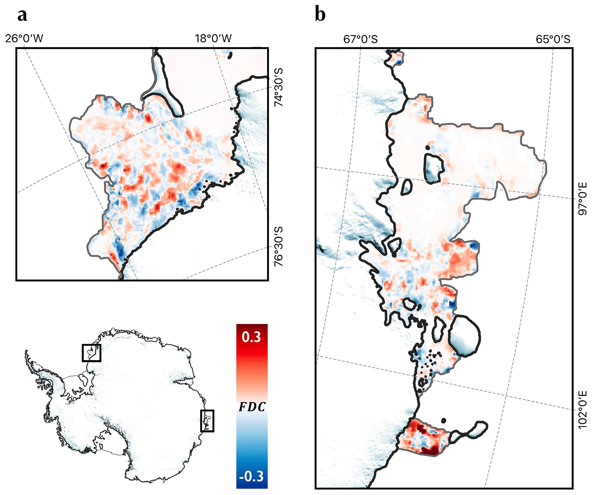
Figure 9Fracture density change in the Brunt–Stancomb–Wills and Shackleton ice shelves. Panel (a) shows the fracture density change in the Brunt–Stancomb–Wills Ice Shelf. Panel (b) shows this for the Shackleton Ice Shelf and surroundings. Locations are shown in the schematic of the Antarctic Ice Sheet in the bottom-left corner. The black lines show the MEaSUREs grounding line (Rignot et al., 2016), and the grey lines delineate the edges of the ice shelves. The interior of the ice sheet is masked with the REMA 2 km DEM (Porter et al., 2018).
4.3 Future work on measuring changes in fracture density
Though our method of measuring the evolution of ice shelf crevassing is capable of resolving severe structural changes in fast-changing regions, few places in Antarctica are changing as rapidly as the Amundsen Sea Embayment (Mouginot et al., 2014; Shepherd et al., 2019). The results of applying this technique to the Antarctic Ice Sheet as a whole would likely be dominated by noise. In some places, such as Crosson Ice Shelf (Fig. 7j), the method may not be particularly useful where change is dominated by the advection of existing crevasses, and “interesting” changes are subtle in comparison. For example, Fig. 9 shows fracture density changes on the Brunt–Stancomb–Wills (BSW) and Shackleton ice shelves. Here, the stripes of positive and negative trends in fracture density show advection on the BSW Ice Shelf and in the Shackleton shear margin, though the steady propagation of Chasm-1 (Libert et al., 2022), for example, is difficult to discern. In future, we could apply Lagrangian corrections to fracture maps before looking at fracture density change or using a method that does not involve averaging over large regions and monitoring the size of isolated rifts.
Finally, future studies should take place investigating alternative means of reducing the component of fracture density time series due to the dependence of crevasse visibility on surface conditions. Our method uses backscatter standard deviation to alias consistent time series and build an ensemble of trends for each location. This is based on the observation that the fracture density and backscatter standard deviation signals appear to respond in the same way to changing firn or ice surface properties. It ought to be possible, for example using a regional climate model or reanalysis data, to better constrain the most salient factors in the environmental contribution to the fracture density signal. These can then be isolated using additional datasets to perform the procedure outlined here more accurately.
4.4 Representation of damage in numerical modelling
The physics of material failure is not well integrated into many large-scale ice sheet models but, through its distributed influence on stress conditions, this omission may have a large impact on predictions of the evolution of the ice sheet. Both the crevasse maps and fracture-density change maps introduced in this article have conceivable use in numerical modelling studies. Firstly, static, pan-continental mosaics of crevasses can be assimilated into numerical models to better constrain initial control parameters for simulations. Specifically, models often require a control parameter specifying changes to the effective ice viscosity from that provided by the ice constitutive relation (Cuffey and Paterson, 2010; Cornford et al., 2015). Given that the presence of fractures is assumed to change the effective ice viscosity, the fracture data can be used to constrain an inverse problem aiming to infer such a field from ice speed data. On grounded ice, these maps could be particularly useful in reducing the underdeterminedness of inversions for both ice softness and basal friction.
It is also conceivable that the smooth, scalar fracture density change maps we produce could be used more directly in diagnostic modelling. In continuum mechanics, a scalar “damage” parameter is often used to represent the reduction in effective ice viscosity caused by the presence of fractures (Lemaitre, 2012; Borstad et al., 2012). The dynamic impact of structural change for glaciers of interest, e.g. Pine Island Glacier, could be investigated by using fracture-density-changed fields as a proxy for damage change.
Additionally, data on the location of crevasses can be used to inform our understanding of the physical processes which lead to crevasse development. In particular, the healing of grounded surface fractures suggests their presence is a function of instantaneous stress conditions rather than a complicated and intractable stress history. This suggests the data could be used to constrain models seeking damage as a function of stress invariants, using stress fields inferred from coincident ice velocity observations. At a more basic level, such data, in combination with accurate vertical stress profiles, could be used to study the fracture toughness of meteoric glacier ice in the interior of the Antarctic Ice Sheet.
4.5 The use of SAR backscatter images
We turn now to a discussion of synthetic aperture radar data as the base dataset for this study. We have shown that a large variety of crevasse-like features are visible in the SAR backscatter images acquired by Sentinel-1 (Fig. 5) and, using parallel processing of the images for type-A and type-B features, that most of these can be automatically extracted in a way reliable enough to promote discussion of existing crevasse patterns and to measure important structural changes on ice shelves. However, there could be choices other than SAR as the base dataset for this work that have the desired spatial coverage, in particular, the use of optical satellite data or a high-resolution digital elevation model (DEM). The further need for a time series of fracture maps leaves optical data as the only appropriate alternative candidate, although this would preclude year-round monitoring during the polar night.
Many but not all of the features we are interested in can be seen in optical imagery of comparable resolution to our SAR data. Crucially, crevasses corresponding to type-B features can rarely be seen reliably in optical imagery, except from in the most high-resolution (<10 m) cases. Even then, they are often bridged by snow. Hence, the use of SAR data allows for the mapping of crevasses on grounded ice, which are essentially exclusively type-B. Additionally, optical imagery, in contrast to SAR data, is hampered by the presence of clouds and cannot acquire images at night or during large parts of the austral winter. SAR data are therefore preferable for generating a consistent, reliable time series which can be used to measure changes to crevassing over relatively short timescales. Of the SAR satellites available, we consider Sentinel-1 to be the best tool due to its pan-continental large-scale acquisition plan which acquires new images every 6 to 12 d. Though it does not have as fine a spatial resolution as some other SAR satellites, such as TerraSAR-X, its short repeat period and extensive spatial coverage allow a consistent time series to be generated that covers the whole Antarctic margin.
There are, however, certain disadvantages to the use of SAR. Some ice shelf crevasses appear smoother on the surface than in optical imagery. For example, the crevasses on Dotson Ice Shelf, which appear faintly in SAR backscatter images at 50 m resolution, can be seen more clearly in the MODIS mosaic of Antarctica (MOA) image over the same region (Haran et al., 2021; Greene et al., 2017). Due to layover and shadowing effects stemming from the fact that SAR images are reconstructed from range distances rather than incidence angles of received radiation, there are additional issues in geolocating crevasses. This is most important for type-B features, where the geocoding errors induced by these effects can be of the order of a crevasse width. However, these are likely to be small in comparison to errors induced by deviations in the surface height through time from those given by the digital elevation model. Most importantly, optical data often come with multi-band information such as different colours in the visible spectrum. We use single-band SAR data due to constraints on the amount of throughput data required to generate pan-continental mosaics. However, as discussed above, the type-A processing fails in the presence of melt ponds. Optical data, in which the water appears blue, or multi-band SAR with dual polarisation, would be useful input to a neural network trying to discern fractures from linear boundaries of these pools of water. Finally, the use of a DEM might allow for the simultaneous extraction of crevasse-location and crevasse-depth data, the latter of which can only be estimated from SAR data.
The detection of crevasses using maps of interferometric fringes (Libert et al., 2022), phase coherence (Hogg and Gudmundsson, 2017) or strain rate fields (De Rydt et al., 2018) comes with additional valuable information on the “activity” of crevasses – where their presence induces discontinuities in certain properties of the ice (e.g. its flow speed). Similarly, the use of precision altimetry data from ICESat-2 provides some information on the depth of crevasses (Herzfeld et al., 2021). The method presented in this work does not provide any such information but, as a consequence, provides more extensive maps of crevasses with much greater coverage. As such, these data are useful for large-scale analyses, studies in regions with low interferometric coherence or imperfect velocity observations, and studies where the activity of the crevasses is of secondary importance – for example as a source of surface-to-bed hydrological pathways. Additionally, a dataset of crevasse locations such as that provided here can be used in combination with such methods to learn more about the importance of different crevasses across the continent. For example, it would be simple to locate ICESat-2 observations coincident with identified crevasses to assess some measure of depth, with the understanding that a reliable estimate of true depth is unattainable in many cases due to the sub-resolution width of the crack tip, or to look for discontinuities in ice shelf flow speed at crevasse locations in coincident velocity observations.
4.6 Future improvements to the crevasse maps
The method of mapping crevasses presented in this work includes different processing chains for detecting the features we call type-A and type-B. This is necessary because of their different appearance in the backscatter images but has the added benefit of providing an independent dataset for each fracture type, which allows for almost independent analysis of crevasses on grounded and floating ice. In order to constrain models of fracture development on ice shelves, it would be useful to further partition the type-A crevasses into basal and surface crevasses. This could be done by tuning the existing type-A network with a small dataset of manually annotated basal and surface crevasses separately and running them in parallel. This would also help solve the current insensitivity of the data to those features which might correspond to basal crevasses.
Improvements to the accuracy of the crevasse mapping can in all likelihood be gained without a great deal of work with the use of SAR data at multiple resolutions. We have been able to present accurate crevasse maps with large spatiotemporal coverage, in part by limiting processing to the use of data at a single spatial resolution, with our choice of 50 m based on a trade-off between the detail at which crevasses can be seen in the data and the finite capacity for computational throughput at our disposal. However, a greater number of crevasses can be seen at 10 m resolution, beyond the limit of what can be achieved with Sentinel-1 backscatter data, which, for example, would allow for more accurate bounding of regions of type-B crevasses.
Our discussions (Sect. 4.5) suggest improvements can be made to the detection of basal crevasses and in discriminating between crevasses and the boundaries of surface melt ponds using multi-band input. We believe the greatest improvements could be seen by combining input SAR data with any available coincident optical data. This could be used to bolster static maps, where time series are not required. Additionally, we note that the sensitivity of the crevasse maps is not enough to capture subtle changes to crevasse density and length. This can be tackled in two ways: increase the sensitivity or increase the timescale of processes of interest. A potential method for the first is to work directly with time-series data. If a neural network were designed to receive as input a sequence of images and to segment the central one, the persistence of features of interest could be learned by the model, leading to more consistent time series. To tackle the second problem, it is feasible to train the network to segment older satellite imagery, e.g. from RADARSat, ENIVSAT or ERS1 and ERS2. This would enable a more extensive analysis of the longer-term (decadal) patterns of change in crevassing over the Antarctic continent.
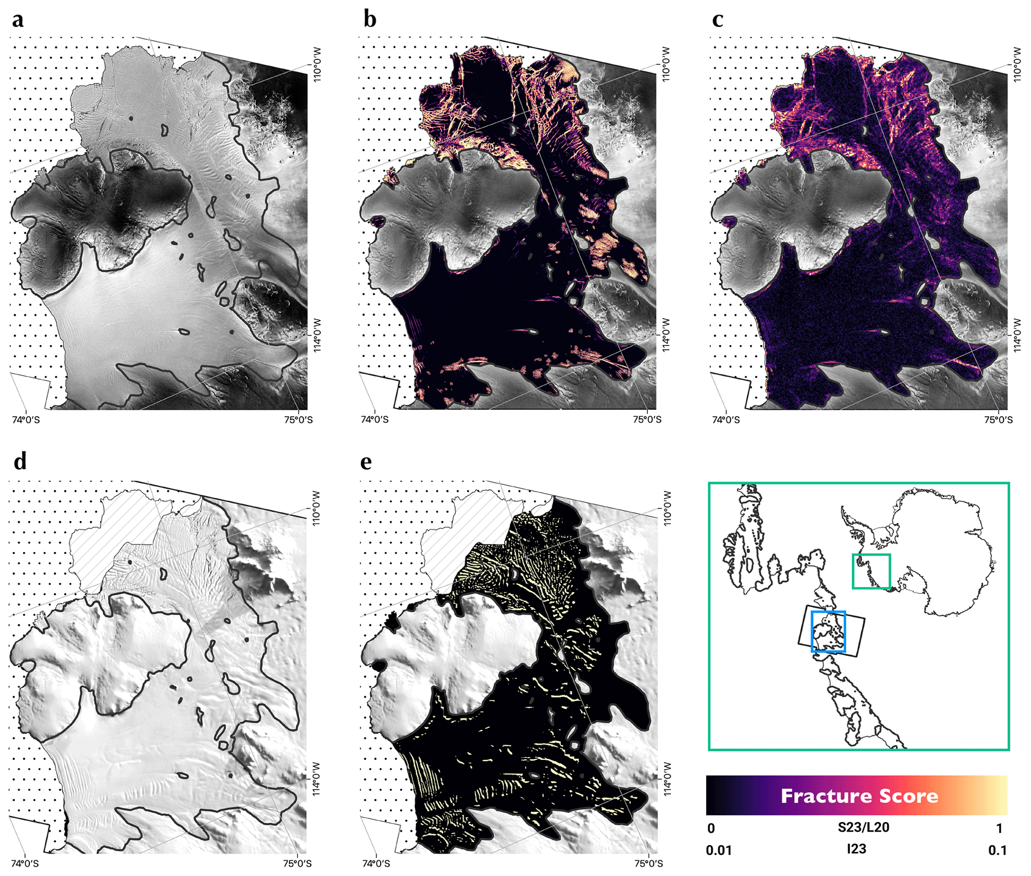
Figure 10A comparison of fracture maps generated using our method (“S23”) versus two existing methods, Lai et al. (2020) “L20” and Izeboud and Lhermitte (2023) “I23”, over the Crosson and Dotson ice shelves. (a) Sentinel-1 backscatter image at 50 m resolution, ESA PF 7/913, dated 7 June 2021 and used for the S23 and I23 crevasse maps. (b) June 2021 crevasse mosaic using S23 restricted to the floating ice. (c) Result of application of I23 to the SAR backscatter image shown in panel (a) with the colour map showing the range 0.01 to 0.1. Grounded ice in panels (b)–(c) is masked by the SAR backscatter image shown in panel (a). (d) MODIS mosaic of Antarctica (Haran et al., 2014) restricted to the geometry of the SAR backscatter image shown in panel (a). (e) Crevasse map from L20 with the grounded ice masked by the MODIS MOA shown in panel (d). The area outside of the bounds of the SAR backscatter image shown in panel (a) is masked in panels (a)–(e). Grounding lines are as given by Rignot et al. (2016) and are shown with a black line. The difference between the June 2021 Crosson Ice Shelf extent and the edge of the L20 dataset is shown in panels (d)–(e) as the striped region. The sea is shown as the spotted region. The blue box in the map in the bottom right shows the extent of the region shown in panels (a)–(e). This lies on a black outline showing the bounds of the SAR backscatter image shown in panel (a). The inset is a map of Antarctica showing the location of the blown-up region. For S23 and L20, the colour map displays the range 0–1, while for I23, it displays the range 0.01–0.1.
4.7 A comparison of ice shelf crevasse detection methods
The crevasse maps presented in this work provide unified coverage over the extent of floating and grounded ice in Antarctica imaged by Sentinel-1. As far as the authors are aware, there are no existing methods with publicly available datasets or code for the large-scale detection of Antarctic surface crevasses on grounded ice. However, methods for crevasse detection on floating ice shelves do exist. We conduct a brief comparison, for a single Sentinel-1 image frame, between the results from the method presented in this work and two publicly available existing datasets and methods, namely those of Lai et al. (2020) and Izeboud and Lhermitte (2023). We refer to these respectively as “L20” and “I23” and to the method presented in this article as “S23”. L20 used U-Net to extract ice shelf crevasses from optical data covering the AIS at 125 m resolution, while I23 used a method based on the normalised radon transform that can be applied to data from different sensors at different resolutions. We applied I23 to a Sentinel-1 backscatter image (Sentinel-1 PF 7/913, dated 7 June 2021) at 50 m resolution using a window size of 10 pixels and a normalisation range of −30 to 0 dB. These are compared with the June 2021 mosaic over the extent of the aforementioned SAR backscatter image. This location (covering the Crosson and Dotson ice shelves of the Amundsen Sea sector of West Antarctica) was chosen again for the variety of crevasse features in the image. Results are shown in Fig. 10. Satellite images from which the data were generated are shown in Fig. 10a and d, and the derived data are shown in panels b, c and e. The SAR image (a) corresponding to data shown in panels b and c is from 7 June 2021, while the MODIS image (d) from which e was derived is constructed from images dating between 2008 and 2009. The outputs corresponding to L20 and S23 are in the range [0,1], while the range for I23 is a parameter that is chosen based on the windows size and image resolution to tune the output to best represent fractures visible in the input image. In this case, we set the bounds to [0.01, 0.1]. We show in Fig. 10 a “fracture score” that uses the same colour map for the outputs of each method but with different bounds.
Overall, with bounds for the range of the I23 dataset to [0.01, 0.1], we see a relatively good agreement between S23 and I23. Both pick up the large-scale patterns of fracture on Crosson Ice Shelf and display relatively little on Dotson Ice Shelf (Fig. 10a–c), though the features in S23 have a higher contrast with lower background noise. The resolution of the I23 output is defined by the window size over which radon transforms are calculated and, with a choice of 10 pixels, S23 improves on this resolution by an order of magnitude, though the comparison might not be fair given the possibility of using I23 with different, higher-resolution sensors. The S23 output is dominated by type-A crevasses, though closer to the grounding line there are fields of type-B fractures in the input SAR backscatter image that can be seen in S23 but not in I23. Finally, we note that the time taken to process this SAR frame was significantly higher in the case of I23 than our method when running with an equal number of processes and the same CPU hardware.
The differences between S23 and L20 are partly due to the evolution of Crosson Ice Shelf in the period 2009 to 2021 (visible in Fig. 10a and d), such as the advection and extension of a large central rift in the ice shelf and the degradation of the northern shear margin that borders Bear Island. However, there are also fundamental differences between these datasets that will influence their future application. Firstly, there is a preference for L20 to extract wider, smoother features over sharp rifts or deep, disordered fractures in the shear margins, while the reverse is true for S23. This leads to a near reversal in the features that are detected between the two methods. On Crosson Ice Shelf, the large central rifts visible in Fig. 10d do not appear in L20 (e), while similar rifts are prominent features in panels a–c. Additionally, the flowband features in L20 (many of which appear not to be crevasses) do not appear in S23. On Dotson Ice Shelf, however, L20 contains a great deal of basal-crevasse-like features visible in panel d which appear only faintly if at all in S23.
Overall, considering ice shelves as well as grounded ice, we would advocate for the use of the data and method presented in this article or a combination of the data presented here and those of Lai et al. (2020) when a single fully comprehensive map of crevasse features is required. This is especially true for continent-wide studies as our data do not cover the majority of the Ronne–Filchner and Ross ice shelves, unlike those of Lai et al. (2020). However, we acknowledge that the comparison presented here is largely qualitative, covers only a small area, and includes only three datasets. Hence, future work should aim to conduct a more exhaustive comparison of existing crevasse-mapping products over a large and varied set of times and ice shelves to explore more completely the benefits and disadvantages of different methods.
We have developed and applied a method of crevasse detection from Sentinel-1 SAR backscatter imagery using convolutional neural networks in combination with parallel-structure filtering. Our results show that crevasses are a major feature of most ice shelves around the Antarctic coastline and much of the grounded ice in shear- and slip-dominated flow regimes. We have developed a method for measuring the change in fracturing on ice shelves over a relatively short timescale, which requires careful consideration of environmental factors that alter the surface expression of crevasses. These results, combined with analysis of the stress conditions using a numerical model, showed changes in the density of crevasses in buttressing regions of ice shelves in the Amundsen Sea Embayment within the 7.5-year study period from 2015 to 2022. We suggest that recent ice dynamic changes to these ice streams likely cannot be fully accounted for without the observed structural changes. On Pine Island Glacier, the changes in fracture density are particularly severe and have occurred largely in a region of high shear stress. As a result, it is likely that change in fracturing has decreased the buttressing capacity of the ice shelf at the grounding line on this major West Antarctic ice stream and is hence also required to explain recent change in grounding line ice mass flux and grounding line location. In the future, we will continue to develop the methods introduced here to differentiate crevasse types and to reduce the uncertainty in the time series of structural change. Future studies must develop an improved physical representation of damage in ice flow models as it is clear that the ice dynamic response cannot be fully reproduced without accounting for change in damage.
The method of extracting locally parallel linear features from the type-B network uses as a starting point the method proposed by Frangi et al. (1998) for finding the likelihood of a pixel lying on a linear structure, using the Hessian matrix local to each pixel. We include the additional step of using the second eigenvector of the Hessian to calculate whether the linear structures we find are near-parallel to others nearby. We call this process “parallel-structure filtering”.
Given a network output 𝒟(x,y), with values at each point between 0 and 1, the Hessian ℋ(x,y) defines the second derivatives at each point. We find the components of ℋ(x,y) by convolving 𝒟 with a full set of Gaussian derivative kernels:
where i and j denote the coordinate directions x or y. The components of 𝒢(x,y) are given by the second derivatives of the two-dimensional Gaussian:
where σ is chosen based on the width of the structures we see in the network outputs.
Frangi et al. (1998) describe an intuitive method of judging the “vesselness” 𝒱 of each pixel (how likely it is to be on part of a linear, tube-like feature of the image) based on the eigenvalues of ℋ(x,y). We use a modification of this described in Jerman et al. (2016). At a particular location, we define the functions B and S of the pixel Hessian eigenvalues as
where .
Because the locations of crevasses are brighter in 𝒟 than the background, when λ2>0, we take the likelihood of the pixel being part of a crevasse feature to be zero. Otherwise, we take
with α=0.5 and .
Setting pixels with 𝒱<0.1 to zero, we then calculate the angle of the linear structure local to each pixel using the eigenvector (corresponding to eigenvalue λ2) that defines the direction along any identified structure:
Finally, we calculate the local variance of the angles:
where is a box kernel of width 71. We mask pixels (x,y) in the original image where or .
This method has been shown to be useful for the detection of type-B crevasses from network outputs and, due to its intuitive nature and use of freely available tools, it could be utilised in any situation in which one is attempting to extract linear features that are locally parallel from relatively noise-free data.
We also note that this method provides us with smooth fields for the orientation of type-B crevasses. At present, this information is not used but could be utilised in future, for example to assess strain rates using measurements at different times.
The approach we take to decouple the part of the signal resulting from real changes in the crevasse pattern and those due to changes in the surface expression of the crevasses resulting from unknown environmental factors is to only compare fracture density data points generated from images showing ice with similar surface properties. We do so by looking directly at the backscatter images of the ice shelves to find sets of dates where the standard deviations of the backscatter signal over the region of interest are comparable. The assumptions that motivate this are that the backscatter standard deviation is dependent on the same surface properties that dominate the fracture density time series, with a small component due to changing fracture patterns, and that there is a close correspondence between a set of surface properties and a particular backscatter standard deviation. Comparing the standard deviation and fracture density time series for a part of the Thwaites Eastern Ice Shelf, where fracturing is increasing, shows the standard deviation mirroring the seasonal features of the fracture-density time series without the accompanying trend (Fig. B1).
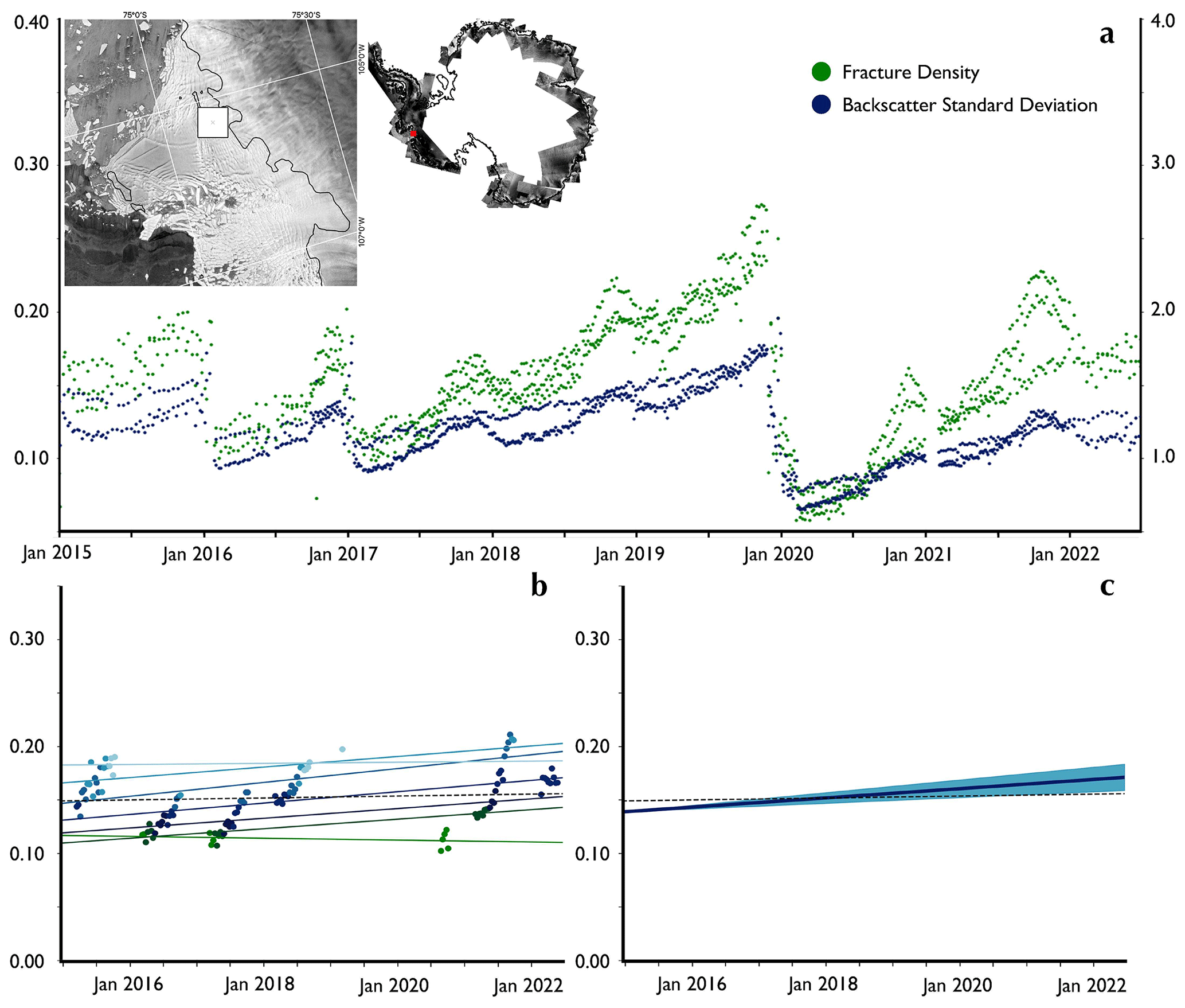
Figure B1Evaluating fracture density change for a point on the Thwaites Eastern Ice Shelf. (a) A time series of fracture density (green) and backscatter standard deviation (blue) for a 10 km×10 km region over the Thwaites Eastern Ice Shelf. Inset: a SAR backscatter image of the Thwaites terminus with the region over which the time series were extracted and highlighted with a white box. To the right is a SAR mosaic from April 2022 with the location of the Thwaites terminus image shown in red. The black lines show the MEaSUREs grounding line (Rignot et al., 2016). (b) Linear trends through an ensemble of data points corresponding to monthly median fracture densities for dates with backscatter standard deviations within 0.1 of each other. Different colours represent different collections of data points. The black dashed line shows the fit through the whole collection of data points without partitioning using backscatter standard deviations. Panel (c) shows the ensemble mean and uncertainty in the fits in panel (b) that result in a fracture density change measurement shown for this location in Fig. 7. The black dashed line shows the same as in panel (b). The figure shows how a non-zero trend is recovered when we apply a correction for surface conditions that is not visible in the original time series.
For a given region, we generate fracture density and backscatter standard deviation time series. For a particular value of standard deviation xi, we find the dates in the time series with standard deviation within a small neighbourhood of xi. This gives us a set of dates in which the ice had similar surface properties. We then find the fracture densities for this set of dates. We perform a linear fit through this set of data points which gives us a y intercept, a gradient and their associated errors: (ci,δci) and (mi,δmi). By stepping through standard deviations, we can, by following the above procedure, build a set of such coefficients.
We report the error-weighted mean and standard deviation of the estimates of the trend, multiplied by the time span
and
where N is the number of estimates.
We use the following scalar field to represent how “buttressed” a region is:
where e2 is the smallest eigenvalue of the vertically integrated viscous stress tensor R and N is the value of the vertically integrated hydrostatic pressure at that location:
ρi is the density of water, ρw is the density of sea water, g is the acceleration due to gravity, and h is the ice thickness (Gudmundsson, 2013; Fürst et al., 2016).
The comparison of N with the second principal viscous stress e2 rather than, for example, the viscous stress in the direction of flow or the first principal viscous stress creates a maximum-valued κ (Fürst et al., 2016), as the eigenvector with eigenvalue e2 defines the direction along which viscous stresses are most compressive. The use of R, rather than, for example, the full Cauchy stress, is convenient as we use a two-dimensional approximation to the ice shelf that boils down to the shallow-shelf approximation (MacAyeal, 1989).
We use the BISICLES ice sheet model (Cornford et al., 2013) to generate fields representing the components of R from observations of ice velocity (Rignot et al., 2017) and ice sheet geometry (Morlighem, 2020; Morlighem et al., 2020). This was done by first solving the inverse problem for a basal drag and ice stiffness parameter on the ice shelves (Cornford et al., 2015) and retrieving the viscous stress tensor given those fields as a by-product. We take the buttressing number at the start of the observational period in order to assess changes to fracture density in regions that had a distributed effect on stresses within the ice shelf before additional crevasses developed.
The authors have made public a Zenodo repository (https://doi.org/10.5281/zenodo.8410599, Surawy-Stepney, 2023) containing a collection of Python and shell scripts, including generation of SAR backscatter images, the application of NA and NB, and the parallel-structure filtering algorithm, which can be used to make fracture maps according to the methods described in this article.
The authors have made available a repository (https://doi.org/10.5281/zenodo.8296992; Surawy-Stepney and Hogg, 2023) that contains a composite fracture map and SAR backscatter image for the month of June 2022 at 100 m resolution together with the January 2015 to July 2022 fracture density change map covering the Amundsen Sea sector and the associated estimate of uncertainty. The authors would be happy to share data on request.
TSS and AEH designed the work. TSS designed the algorithms and processing chains described in the article, wrote the code that implements them, and wrote the manuscript. SLC and DCH respectively provided advice on modelling and computer vision methods. All the authors contributed suggestions to the manuscript.
The contact author has declared that none of the authors has any competing interests.
Publisher's note: Copernicus Publications remains neutral with regard to jurisdictional claims in published maps and institutional affiliations.
This work was led by Trystan Surawy-Stepney at the School of Earth and Environment at the University of Leeds. Much of this work was undertaken on ARC3 and ARC4, part of the High-Performance Computing facilities at the University of Leeds, UK. The authors gratefully acknowledge the ESA and the European Commission for the acquisition of Sentinel-1 data.
This research has been supported by the National Centre for Earth Observation (grant no. NE/T012757/1), the European Space Agency (grant no. ESA-IPLPOE-EF-cb-LE-2019-834) and the Horizon 2020 research and innovation programme (grant no. 869304).
This paper was edited by Kristin Poinar and reviewed by two anonymous referees.
Albrecht, T. and Levermann, A.: Fracture field for large-scale ice dynamics, J. Glaciol., 58, 165–176, https://doi.org/10.3189/2012JoG11J191, 2012. a
Alley, K., Scambos, T., Miller, J., Long, D., and MacFerrin, M.: Quantifying vulnerability of Antarctic ice shelves to hydrofracture using microwave scattering properties, Remote Sens. Environ., 210, 297–306, https://doi.org/10.1016/j.rse.2018.03.025, 2018. a
Alley, K. E., Scambos, T. A., Alley, R. B., and Holschuh, N.: Troughs developed in ice-stream shear margins precondition ice shelves for ocean-driven breakup, Sci. Adv., 5, eaax2215, https://doi.org/10.1126/sciadv.aax2215, 2019. a
Bassis, J. and Ma, Y.: Evolution of basal crevasses links ice shelf stability to ocean forcing, Earth Planet. Sc. Lett., 409, 203–211, https://doi.org/10.1016/j.epsl.2014.11.003, 2015. a
Benn, D. I. and Evans, D. J.: Glaciers & glaciation, Routledge, https://doi.org/10.4324/9780203785010, 2014. a, b
Benn, D. I., Luckman, A., Åström, J. A., Crawford, A. J., Cornford, S. L., Bevan, S. L., Zwinger, T., Gladstone, R., Alley, K., Pettit, E., and Bassis, J.: Rapid fragmentation of Thwaites Eastern Ice Shelf, The Cryosphere, 16, 2545–2564, https://doi.org/10.5194/tc-16-2545-2022, 2022. a, b, c
Borstad, C. P., Khazendar, A., Larour, E., Morlighem, M., Rignot, E., Schodlok, M. P., and Seroussi, H.: A damage mechanics assessment of the Larsen B ice shelf prior to collapse: Toward a physically-based calving law, Geophys. Res. Lett., 39, 18, https://doi.org/10.1029/2012GL053317, 2012. a, b
Colgan, W., Rajaram, H., Abdalati, W., McCutchan, C., Mottram, R., Moussavi, M. S., and Grigsby, S.: Glacier crevasses: Observations, models, and mass balance implications, Rev. Geophys., 54, 119–161, https://doi.org/10.1002/2015RG000504, 2016. a
Cornford, S. L., Martin, D. F., Graves, D. T., Ranken, D. F., Le Brocq, A. M., Gladstone, R. M., Payne, A. J., Ng, E. G., and Lipscomb, W. H.: Adaptive mesh, finite volume modeling of marine ice sheets, J. Comput. Phys., 232, 529–549, https://doi.org/10.1016/j.jcp.2012.08.037, 2013. a
Cornford, S. L., Martin, D. F., Payne, A. J., Ng, E. G., Le Brocq, A. M., Gladstone, R. M., Edwards, T. L., Shannon, S. R., Agosta, C., van den Broeke, M. R., Hellmer, H. H., Krinner, G., Ligtenberg, S. R. M., Timmermann, R., and Vaughan, D. G.: Century-scale simulations of the response of the West Antarctic Ice Sheet to a warming climate, The Cryosphere, 9, 1579–1600, https://doi.org/10.5194/tc-9-1579-2015, 2015. a, b
Cuffey, K. M. and Paterson, W. S. B.: The physics of glaciers, Academic Press, https://doi.org/10.1016/B978-0-12-369461-4.00000-0, ISBN 9780123694614, 2010. a
Davison, B. J., Hogg, A. E., Rigby, R., S, E., van Wessem, J. M., van den Broke, M., Holland, P. R., Selley, H. L., and Dutrieux, P.: Sea level rise from West Antarctic mass loss significantly modified by large snowfall anomalies, Nat. Commun., 14, 1479, https://doi.org/10.1038/s41467-023-36990-3, 2023. a, b
De Rydt, J., Gudmundsson, G. H., Nagler, T., Wuite, J., and King, E. C.: Recent rift formation and impact on the structural integrity of the Brunt Ice Shelf, East Antarctica, The Cryosphere, 12, 505–520, https://doi.org/10.5194/tc-12-505-2018, 2018. a, b
Frangi, A. F., Niessen, W. J., Vincken, K. L., and Viergever, M. A.: Multiscale vessel enhancement filtering, in: Medical Image Computing and Computer-Assisted Intervention – MICCAI'98, edited by: Wells, W. M., Colchester, A., and Delp, S., Springer Berlin Heidelberg, Berlin, Heidelberg, 130–137, https://doi.org/10.1007/BFb0056195, 1998. a, b, c
Fürst, J. J., Durand, G., Gillet-Chaulet, F., Tavard, L., Rankl, M., Braun, M., and Gagliardini, O.: The safety band of Antarctic ice shelves, Nat. Clim. Change, 6, 479–482, https://doi.org/10.1038/nclimate2912, 2016. a, b, c
Gourmelen, N., Goldberg, D. N., Snow, K., Henley, S. F., Bingham, R. G., Kimura, S., Hogg, A. E., Shepherd, A., Mouginot, J., Lenaerts, J. T. M., Ligtenberg, S. R. M., and van de Berg, W. J.: Channelized Melting Drives Thinning Under a Rapidly Melting Antarctic Ice Shelf, Geophys. Res. Lett., 44, 9796–9804, https://doi.org/10.1002/2017GL074929, 2017. a
Greene, C. A., Gwyther, D. E., and Blankenship, D. D.: Antarctic Mapping Tools for Matlab, Comput. Geosci., 104, 151–157, https://doi.org/10.1016/j.cageo.2016.08.003, 2017. a, b, c, d
Gudmundsson, G. H.: Ice-shelf buttressing and the stability of marine ice sheets, The Cryosphere, 7, 647–655, https://doi.org/10.5194/tc-7-647-2013, 2013. a, b
Hambrey, M. and Müller, F.: Structures and Ice Deformation in the White Glacier, Axel Heiberg Island, Northwest Territories, Canada, J. Glaciol., 20, 41–66, https://doi.org/10.3189/S0022143000021213, 1978. a
Haran, T., Bohlander, J., Scambos, T., Painter, T., and Fahnestock, M.: MODIS Mosaic of Antarctica 2008–2009 (MOA2009) Image Map, Version 1, National Snow and Ice Data Center [data set], https://doi.org/10.7265/N5KP8037 (last access: 15 August 2023), 2014. a
Haran, T. M., Bohlander, J., Scambos, T. A., Painter, T. H., and Fahnestock, M. A.: MODIS Mosaic of Antarctica 2003–2004 (MOA2004) Image Map, Version 2, National Snow and Ice Data Center [data set], https://doi.org/10.5067/68TBT0CGJSOJ (last access: 15 August 2023), 2021. a, b, c, d, e
Herzfeld, U. C., Trantow, T., Lawson, M., Hans, J., and Medley, G.: Surface heights and crevasse morphologies of surging and fast-moving glaciers from ICESat-2 laser altimeter data – Application of the density-dimension algorithm (DDA-ice) and evaluation using airborne altimeter and Planet SkySat data, Sci. Remote Sens., 3, 100013, https://doi.org/10.1016/j.srs.2020.100013, 2021. a
Hogg, A. E. and Gudmundsson, G. H.: Impacts of the Larsen-C Ice Shelf calving event, Nat. Clim. Change, 7, 540–542, https://doi.org/10.1038/nclimate3359, 2017. a, b
Hughes, T.: On the Disintegration of Ice Shelves: The Role of Fracture, J. Glaciol., 29, 98–117, https://doi.org/10.3189/S0022143000005177, 1983. a
Hulbe, C. L., LeDoux, C., and Cruikshank, K.: Propagation of long fractures in the Ronne Ice Shelf, Antarctica, investigated using a numerical model of fracture propagation, J. Glaciol., 56, 459–472, https://doi.org/10.3189/002214310792447743, 2010. a
Irwin, G. R.: Analysis of stresses and strains near the end of a crack traversing a plate, J. Appl. Mech., 24, 361–364, https://doi.org/10.1115/1.4011547, 1957. a
Izeboud, M. and Lhermitte, S.: Damage detection on antarctic ice shelves using the normalised radon transform, Remote Sens. Environ., 284, 113359, https://doi.org/10.1016/j.rse.2022.113359, 2023. a, b, c
Jerman, T., Pernuš, F., Likar, B., and Špiclin, V.: Enhancement of Vascular Structures in 3D and 2D Angiographic Images, IEEE T. Med. Imaging, 35, 2107–2118, https://doi.org/10.1109/TMI.2016.2550102, 2016. a, b
Joughin, I., Smith, B. E., and Medley, B.: Marine Ice Sheet Collapse Potentially Under Way for the Thwaites Glacier Basin, West Antarctica, Science, 344, 735–738, https://doi.org/10.1126/science.1249055, 2014. a
Joughin, I., Shapero, D., Smith, B., Dutrieux, P., and Barham, M.: Ice-shelf retreat drives recent Pine Island Glacier speedup, Sci. Adv., 7, eabg3080, https://doi.org/10.1126/sciadv.abg3080, 2021. a, b, c
Konrad, H., Gilbert, L., Cornford, S. L., Payne, A., Hogg, A., Muir, A., and Shepherd, A.: Uneven onset and pace of ice-dynamical imbalance in the Amundsen Sea Embayment, West Antarctica, Geophys. Res. Lett., 44, 910–918, https://doi.org/10.1002/2016GL070733, 2017. a
Lai, C.-Y., Kingslake, J., Wearing, M. G., Chen, P.-H. C., Gentine, P., Li, H., Spergel, J. J., and van Wessem, J. M.: Vulnerability of Antarctica's ice shelves to meltwater-driven fracture, Nature, 584, 574–578, https://doi.org/10.1038/s41586-020-2627-8, 2020. a, b, c, d, e, f, g
Lemaitre, J.: A course on damage mechanics, Springer Science & Business Media, https://doi.org/10.1007/978-3-642-18255-6, 2012. a, b
Lhermitte, S., Sun, S., Shuman, C., Wouters, B., Pattyn, F., Wuite, J., Berthier, E., and Nagler, T.: Damage accelerates ice shelf instability and mass loss in Amundsen Sea Embayment, P. Natl. Acad. Sci. USA, 117, 24735–24741, https://doi.org/10.1073/pnas.1912890117, 2020. a, b, c, d
Libert, L., Wuite, J., and Nagler, T.: Automatic delineation of cracks with Sentinel-1 interferometry for monitoring ice shelf damage and calving, The Cryosphere, 16, 1523–1542, https://doi.org/10.5194/tc-16-1523-2022, 2022. a, b, c
Luckman, A., Jansen, D., Kulessa, B., King, E. C., Sammonds, P., and Benn, D. I.: Basal crevasses in Larsen C Ice Shelf and implications for their global abundance, The Cryosphere, 6, 113–123, https://doi.org/10.5194/tc-6-113-2012, 2012. a
MacAyeal, D. R.: Large-scale ice flow over a viscous basal sediment: Theory and application to ice stream B, Antarctica, J. Geophys. Res.-Sol. Ea., 94, 4071–4087, https://doi.org/10.1029/JB094iB04p04071, 1989. a, b
MacGregor, J. A., Catania, G. A., Markowski, M. S., and Andrews, A. G.: Widespread rifting and retreat of ice-shelf margins in the eastern Amundsen Sea Embayment between 1972 and 2011, J. Glaciol., 58, 458–466, https://doi.org/10.3189/2012JoG11J262, 2012. a, b, c
Marsh, O., Price, D., Courville, Z., and Floricioiu, D.: Crevasse and rift detection in Antarctica from TerraSAR-X satellite imagery, Cold Reg. Sci. Technol., 187, 103284, https://doi.org/10.1016/j.coldregions.2021.103284, 2021. a, b, c
McGrath, D., Steffen, K., Scambos, T., Rajaram, H., Casassa, G., and Rodriguez Lagos, J. L.: Basal crevasses and associated surface crevassing on the Larsen C ice shelf, Antarctica, and their role in ice-shelf instability, Ann. Glaciol., 53, 10–18, https://doi.org/10.3189/2012AoG60A005, 2012. a
Miles, B. W. J., Stokes, C. R., Jenkins, A., Jordan, J. R., Jamieson, S. S. R., and Gudmundsson, G. H.: Intermittent structural weakening and acceleration of the Thwaites Glacier Tongue between 2000 and 2018, J. Glaciol., 66, 485–495, https://doi.org/10.1017/jog.2020.20, 2020. a
Moctezuma-Flores, M. and Parmiggiani, F.: SAR observations of the Nansen Ice Shelf fracture, The European Physical Journal Plus, 131, 1–5, https://doi.org/10.1140/epjp/i2016-16384-y, 2016. a
Morlighem, M.: MEaSUREs BedMachine Antarctica, Version 2 (bed, thickness), Boulder, Colorado USA. NASA National Snow and Ice Data Center Distributed Active Archive Center [data set], https://doi.org/10.5067/E1QL9HFQ7A8M (last access: 5 October 2021), 2020. a
Morlighem, M., Rignot, E., Binder, T., Blankenship, D., Drews, R., Eagles, G., Eisen., O, Ferraccioli, F., Forsberg, R., Fretwell, P., Goel, V., Greenbaum, J. S., Gudmundsson, H., Guo, J., Helm, V., Hofstede, C., Howat, I., Humbert, A., Jokat, W., Karlsson, N. B., Lee, W. S., Matsuoka, K., Millan, R., Mouginot, J., Paden, J., Pattyn, F., Roberts, J., Rosier, S., Ruppel, A., Seroussi, H., Smith, E. C., Steinhage, D., Sun, B., van den Broeke, M. R., van Ommen, T. D., van Wessem, M., and Young, D. A.: Deep glacial troughs and stabilizing ridges unveiled beneath the margins of the Antarctic ice sheet, Nat. Geosci., 13, 132–137, https://doi.org/10.1038/s41561-019-0510-8, 2020. a
Mouginot, J., Scheuchl, B., and Rignot, E.: Mapping of Ice Motion in Antarctica Using Synthetic-Aperture Radar Data, Remote Sens., 4, 2753–2767, https://doi.org/10.3390/rs4092753, 2012. a
Mouginot, J., Rignot, E., and Scheuchl, B.: Sustained increase in ice discharge from the Amundsen Sea Embayment, West Antarctica, from 1973 to 2013, Geophys. Res. Lett., 41, 1576–1584, https://doi.org/10.1002/2013GL059069, 2014. a, b, c
Pfeffer, W. T. and Bretherton, C. S.: The effect of crevasses on the solar heating of a glacier surface, IAHS Publ, 170, 191–205, 1987. a
Porter, C., Morin, P., Howat, I., Noh, M.-J., Bates, B., Peterman, K., Keesey, S., Schlenk, M., Gardiner, J., Tomko, K., Willis, M., Kelleher, C., Cloutier, M., Husby, E., Foga, S., Nakamura, H., Platson, M., Wethington, Michael, J., Williamson, C., Bauer, G., Enos, J., Arnold, G., Kramer, W., Becker, P., Doshi, A., D'Souza, C., Cummens, P., Laurier, F., and Bojesen, M.: ArcticDEM, Version 3, Harvard Dataverse [data set], https://doi.org/10.7910/DVN/OHHUKH (last access: 10 June 2021), 2018. a, b, c
Pralong, A. and Funk, M.: Dynamic damage model of crevasse opening and application to glacier calving, J. Geophys. Res.-Sol. Ea., 110, B1, https://doi.org/10.1029/2004JB003104, 2005. a
Purdie, H., Zawar-Reza, P., Katurji, M., Schumacher, B., Kerr, T., and Bealing, P.: Variability in the vertical temperature profile within crevasses at an alpine glacier, J. Glaciol., 69, 410–424, https://doi.org/10.1017/jog.2022.73, 2022. a
Rignot, E., Mouginot, J., and Scheuchl, B.: MEaSUREs Antarctic Grounding Line from Differential Satellite Radar Interferometry, Version 2, boulder, Colorado USA. NASA National Snow and Ice Data Center Distributed Active Archive Center [data set], https://doi.org/10.5067/IKBWW4RYHF1Q (last access: 15 January 2021), 2016. a, b, c, d, e, f, g, h, i, j
Rignot, E., Mouginot, J., and Scheuchl, B.: MEaSUREs InSAR-Based Antarctica Ice Velocity Map, Version 2, National Snow and Ice Data Center [data set], https://doi.org/10.5067/D7GK8F5J8M8R (last access: 5 October 2021), 2017. a, b
Ronneberger, O., Fischer, P., and Brox, T.: U-Net: Convolutional Networks for Biomedical Image Segmentation, in: Medical Image Computing and Computer-Assisted Intervention – MICCAI 2015, edited by: Navab, N., Hornegger, J., Wells, W. M., and Frangi, A. F., 234–241, Springer International Publishing, Cham, https://doi.org/10.1007/978-3-319-24574-4_28, 2015. a
Rott, H., Skvarca, P., and Nagler, T.: Rapid Collapse of Northern Larsen Ice Shelf, Antarctica, Science, 271, 788–792, https://doi.org/10.1126/science.271.5250.788, 1996. a
Scambos, T., Fricker, H. A., Liu, C.-C., Bohlander, J., Fastook, J., Sargent, A., Massom, R., and Wu, A.-M.: Ice shelf disintegration by plate bending and hydro-fracture: Satellite observations and model results of the 2008 Wilkins ice shelf break-ups, Earth Planet. Sc. Lett., 280, 51–60, https://doi.org/10.1016/j.epsl.2008.12.027, 2009. a
Shepherd, A., Wingham, D., and Rignot, E.: Warm ocean is eroding West Antarctic Ice Sheet, Geophys. Res. Lett., 31, 23, https://doi.org/10.1029/2004GL021106, 2004. a
Shepherd, A., Gilbert, L., Muir, A. S., Konrad, H., McMillan, M., Slater, T., Briggs, K. H., Sundal, A. V., Hogg, A. E., and Engdahl, M. E.: Trends in Antarctic Ice Sheet Elevation and Mass, Geophys. Res. Lett., 46, 8174–8183, https://doi.org/10.1029/2019GL082182, 2019. a
Surawy-Stepney, T.: Code accompanying the article “Mapping Antarctic Crevasses and their Evolution with Deep Learning Applied to Satellite Radar Imagery” (Version 1), Zenodo [code], https://doi.org/10.5281/zenodo.8410599, 2023. a
Surawy-Stepney, T. and Hogg, A. E.: Data accompanying the article “Mapping Antarctic Crevasses and their Evolution with Deep Learning Applied to Satellite Radar Imagery” (Version 1), Zenodo [data set], https://doi.org/10.5281/zenodo.8296992 (last access: 3 March 2023), 2023. a
Surawy-Stepney, T., Hogg, A. E., Cornford, S. L., and Davison, B. J.: Episodic dynamic change linked to damage on the thwaites glacier ice tongue, Nat. Geosci., 16, 37–43, https://doi.org/10.1038/s41561-022-01097-9, 2023. a, b, c, d, e, f, g, h
Thompson, S., Cook, S., Kulessa, B., Winberry, J., Fraser, A., and Galton-Fenzi, B.: Comparing satellite and helicopter-based methods for observing crevasses, application in East Antarctica, Cold Reg. Sci. Technol., 178, 103128, https://doi.org/10.1016/j.coldregions.2020.103128, 2020. a, b
Vaughan, D. G., Corr, H. F. J., Bindschadler, R. A., Dutrieux, P., Gudmundsson, G. H., Jenkins, A., Newman, T., Vornberger, P., and Wingham, D. J.: Subglacial melt channels and fracture in the floating part of Pine Island Glacier, Antarctica, J. Geophys. Res.-Earth Surf., 117, F3, https://doi.org/10.1029/2012JF002360, 2012. a, b
Zhao, J., Liang, S., Li, X., Duan, Y., and Liang, L.: Detection of Surface Crevasses over Antarctic Ice Shelves Using SAR Imagery and Deep Learning Method, Remote Sens., 14, 487, https://doi.org/10.3390/rs14030487, 2022. a, b
- Abstract
- Introduction
- Identifying crevasses
- Measuring changes in fracture density
- Discussion
- Conclusions
- Appendix A: Parallel-structure filtering
- Appendix B: Measuring trends in fracture density
- Appendix C: Calculating the buttressing number
- Code availability
- Data availability
- Author contributions
- Competing interests
- Disclaimer
- Acknowledgements
- Financial support
- Review statement
- References