the Creative Commons Attribution 4.0 License.
the Creative Commons Attribution 4.0 License.
 | 06 Oct 2023
Sensitivity of the MAR regional climate model snowpack to the parameterization of the assimilation of satellite-derived wet-snow masks on the Antarctic Peninsula
Quentin Glaude
Ghislain Picard
Christoph Kittel
Patrick Alexander
Anne Orban
Xavier Fettweis
Both regional climate models (RCMs) and remote sensing (RS) data are essential tools in understanding the response of polar regions to climate change. RCMs can simulate how certain climate variables, such as surface melt, runoff and snowfall, are likely to change in response to different climate scenarios but are subject to biases and errors. RS data can assist in reducing and quantifying model uncertainties by providing indirect observations of the modeled variables on the present climate. In this work, we improve on an existing scheme to assimilate RS wet snow occurrence data with the “Modèle Atmosphérique Régional” (MAR) RCM and investigate the sensitivity of the RCM to the parameters of the scheme. The assimilation is performed by nudging the MAR snowpack temperature to match the presence of liquid water observed by satellites. The sensitivity of the assimilation method is tested by modifying parameters such as the depth to which the MAR snowpack is warmed or cooled, the quantity of water required to qualify a MAR pixel as “wet” (0.1 % or 0.2 % of the snowpack mass being water), and assimilating different RS datasets. Data assimilation is carried out on the Antarctic Peninsula for the 2019–2021 period. The results show an increase in meltwater production (+66.7 % on average, or +95 Gt), along with a small decrease in surface mass balance (SMB) (−4.5 % on average, or −20 Gt) for the 2019–2020 melt season after assimilation. The model is sensitive to the tested parameters, albeit with varying orders of magnitude. The prescribed warming depth has a larger impact on the resulting surface melt production than the liquid water content (LWC) threshold due to strong refreezing occurring within the top layers of the snowpack. The values tested for the LWC threshold are lower than the LWC for typical melt days (approximately 1.2 %) and impact results mainly at the beginning and end of the melting period. The assimilation method will allow for the estimation of uncertainty in MAR meltwater production and will enable the identification of potential issues in modeling near-surface snowpack processes, paving the way for more accurate simulations of snow processes in model projections.
- Article
(6228 KB) - Full-text XML
-
Supplement
(2522 KB) - BibTeX
- EndNote


More than two-thirds of Earth's fresh water is held in the polar ice sheets (Church et al., 2013), with the majority of it trapped as land ice at the south pole, forming the Antarctic Ice Sheet (AIS). According to Fretwell et al. (2013), if all AIS ice were to melt, the global mean sea level would rise by 56 m. Currently, the AIS is primarily losing mass due to grounded ice flowing into the ocean. There, the ice is lost mainly through a combination of basal melting and calving (The IMBIE Team, 2018; Rignot et al., 2019; Adusumilli et al., 2020).
However, the surface melt production on the ice sheet is also important for several reasons. Even moderate surface melt over the ice shelves, the floating boundaries of the ice sheet, is thought to weaken the shelf structure and to cause ponding and hydrofracturing, leading to substantial mass loss (Scambos et al., 2003; Lai et al., 2020). Additionally, surface melting is becoming a growing concern as it may increase greatly with climate change (Trusel et al., 2015; Bell et al., 2018; Gilbert and Kittel, 2021). Ice shelves exert a buttressing effect on the upstream ice flow, regulating the amount of ice that reaches the surrounding ocean. As they thin or collapse, this buttressing effect is reduced (Favier and Pattyn, 2015; Paolo et al., 2015), and AIS ice flow velocity and mass loss are increased.
Climate models are currently one of the most useful tools in studying polar climate evolution. Some of them also include the possibility of modeling the evolution of the snowpack. A notable example is MAR (for “Modèle Atmosphérique Régional” in French), a regional climate model (RCM) specially developed to monitor the polar climate and the surface mass balance of both ice sheets.
Proper surface melt modeling is required to study conditions leading to ice shelf destabilization, as hydrofracturing is impacted by the melting-to-snowfall ratio and the capacity of the snowpack to retain and refreeze meltwater (Donat-Magnin et al., 2021; Gilbert and Kittel, 2021). Additionally, accurate modeling of surface melt is necessary to study the evolution of the snowpack during strong melt events. Studying the ability of the snowpack to retain liquid water is crucial because under higher melt conditions the Antarctic snowpack could saturate and stop absorbing surface meltwater in the future, as has been modeled to occur over the Greenland Ice Sheet (Noël et al., 2017).
Despite their ability to capture snowpack melt at a high level of detail, RCMs still have some limitations. Because of uncertainty in forcing or limitations in physical assumptions, the models may contain significant uncertainties. These uncertainties can be mitigated by employing external data that are not already incorporated into the model to improve its accuracy at specific points in space and/or time. This technique is known as “data assimilation” and is commonly applied in numerous fields where observations can be integrated into a model (Evensen, 2009; Navari et al., 2018).
The assimilation of data into the model is a crucial step in quantifying the uncertainties associated with the model output without assimilation. The assimilation process helps to identify areas and periods where the simulations are not consistent with the observations. This can help us to better understand the underlying physical processes and their interactions. Accordingly, data assimilation provides a powerful tool for improving the reliability of models. In our case, it is an essential step in the process of model refinement, leading to improved predictions from future scenarios.
The highly uneven topography of a region is challenging for RCMs, which typically operate at a resolution on the order of 10 km. Phenomena depending on very local conditions, such as melt induced by the Foehn effect, can occur at smaller spatial scales than the spatial resolution of RCMs and thus may not be captured by the model (Datta et al., 2019; Chuter et al., 2022; Wille et al., 2022). However, high-resolution satellites can document localized or extreme events that may be missed by RCM simulations.
In this paper, we assimilate satellite-derived binary wet-snow masks (wet or non-wet) over the Antarctic Peninsula (AP) in West Antarctica into the MAR model for two melt seasons (2019–2020 and 2020–2021). Three major ice shelves are located on the AP: Larsen C, George VI and Wilkins (Fig. 1). The ice shelves experience the highest amount of surface melt compared to the other part of the AIS, and their surface hydrological processes are also complex and poorly understood (Barrand et al., 2013; Datta et al., 2018; Johnson et al., 2020). Presently, assimilating remotely sensed products in RCMs is a promising method of quantifying surface meltwater production in Antarctica. The scarcity of field observations and the complexity of surface hydrology (Bell et al., 2018) make it difficult to evaluate and constrain models otherwise.
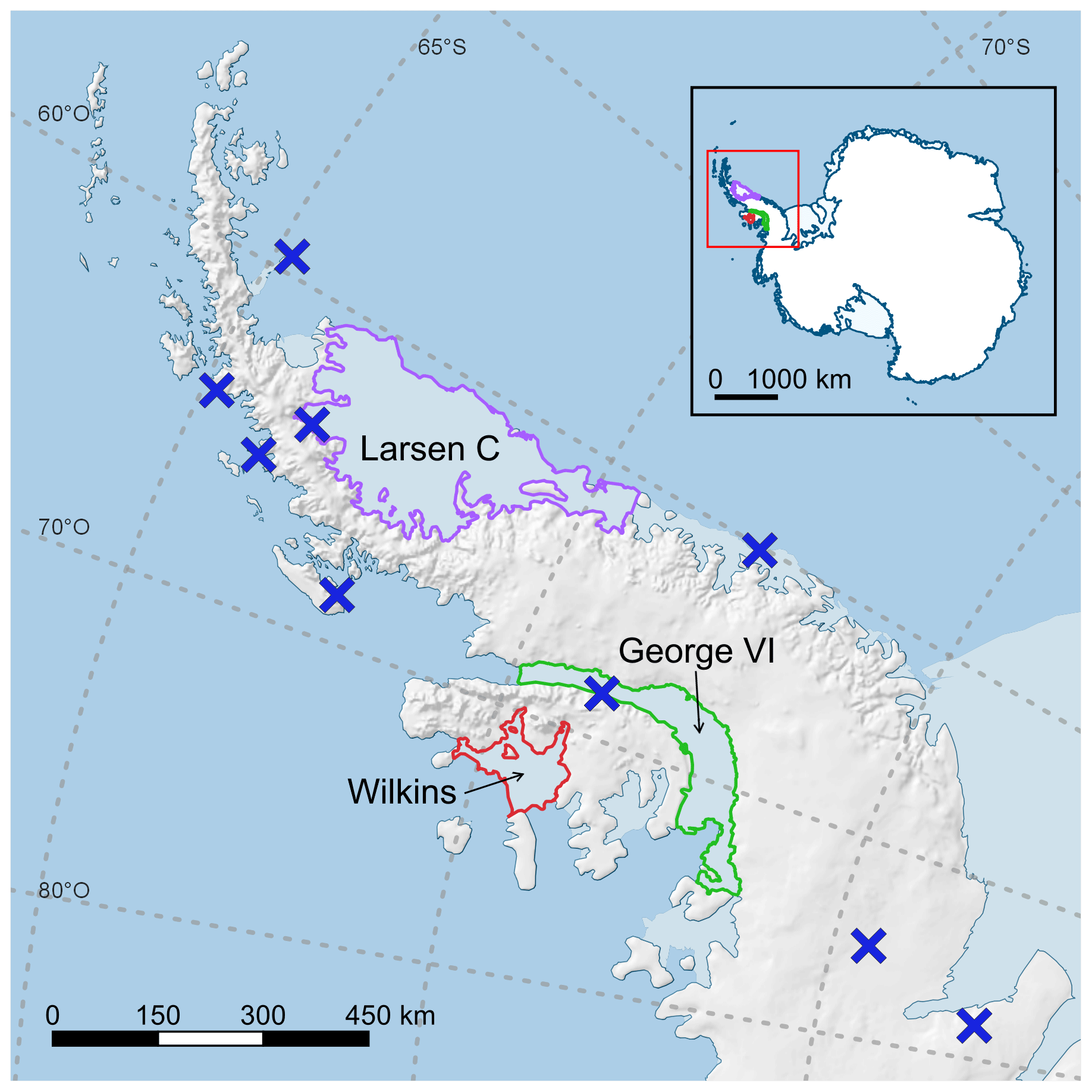
Figure 1The Antarctic Peninsula and three ice shelves examined in this study. The ice shelves are denoted by color outlines. Larsen C is outlined in purple, George VI in green and Wilkins in red. Blue crosses indicate the position of the weather stations used for the model's evaluation (Sect. 3). The red square around the Antarctic Peninsula corresponds to the MAR spatial extent.
The assimilation algorithm performed in this paper is derived from the framework described in Kittel et al. (2022) where the MAR near-surface snowpack is warmed or cooled to best match satellite-derived wet-snow masks. In this study, sensitivity experiments have been performed by varying the depth to which the snowpack temperature is changed (called the assimilation depth hereafter), the minimum liquid water content (LWC) threshold used to classify the modeled snowpack state as “wet”, and the wet-snow satellite product to test the sensitivity of the model to the assimilation.
The satellite data, the model, and the assimilation method are presented in Sect. 2. The validation of the model is described in Sect. 3. The results of the data assimilation sensitivity tests are discussed in Sect. 4. Finally, general conclusions and discussion on assimilation of remote sensing data into the MAR model are included in Sect. 5.
2.1 Satellite data
Depending on the region of interest, the length of the simulation or the spatial resolution, the use of one specific satellite dataset over another for assimilation can be useful. However, depending on the sensor type and acquisition times, the derived wet-snow occurrence can differ between satellites and sensors (Husman et al., 2022). Some sensors operate at a coarser resolution and provide information with higher uncertainty in areas with complex topography, but can provide long time series of daily images using wet snow detection algorithms that have proven to be efficient (Zwally and Fiegles, 1994; Colosio et al., 2021). Other sensors have a better spatial resolution but may have a lower revisit time. The choice of the satellite dataset can thus influence the results of the assimilated model.
We employed three satellite datasets (Table 1) to create the binary (dry/wet) snow masks to be assimilated. The three datasets are derived from sensors operating in the microwave spectrum (at GHz frequencies). Among them, AMSR2 is a “passive sensor”, which records Earth's natural radiation, while the other two are classified as “active” since they actively emit electromagnetic pulses to illuminate the area covered by the satellite. Microwave sensors are commonly used to map snow cover, sea ice, or wet snow extent over ice sheets (Parkinson, 2001; Colosio et al., 2021). The presence of liquid water in the snowpack induces a change in its emissivity and absorptivity. This change leads to a change in the satellite measurements: the backscattering coefficient σ0 for active sensors and the brightness temperature for passive sensors (Zwally and Fiegles, 1994; Johnson et al., 2022; Picard et al., 2022). In this study, the presence of wet snow detected by satellites is interpreted as the presence of liquid water underneath or at the surface of the snowpack. Using microwave data also brings other advantages, such as atmospheric transparency and acquisitions during both day and night. However, the lower spatial resolution of passive microwave sensors (generally 10 to 50 km) compared with active sensors (10 m–5 km) is problematic in identifying small-scale melting (Datta et al., 2018). Finally, with pixels of ∼100 km2 (e.g., for AMSR2; see Table 1), a majority of the pixels cover regions with sub-pixel variations in land cover or surface height (Johnson et al., 2020).
ESA (2023)EUMETSAT (2023)JAXA (2021)Table 1Technical specifications of the remote sensing datasets employed for the assimilation. Datasets are referred to by the name in bold characters in the paper.
2.1.1 Advanced Microwave Scanning Radiometer 2 (AMSR2)
The first dataset employed in this study is from the Advanced Microwave Scanning Radiometer 2 (AMSR2) aboard the Global Change Observation Mission – Water “SHIZUKU” (GCOM-W1) retrieved from the Japan Aerospace Exploration Agency (JAXA) G-Portal (JAXA, 2021). Thanks to a sun-synchronous orbit at an altitude of 700 km and a large swath, AMSR2 obtains low-resolution daily observations of the polar regions. We used the level-3 products containing the daily mean brightness temperature at a horizontal polarization in the 18.7 GHz channel, resampled at a 10 km resolution. The 18.7 GHz channel is used as it is slightly more sensitive to liquid water content than the other frequencies (Picard et al., 2022). Ascending (south to north) and descending (north to south) satellite paths were processed separately, as they happen in the morning and in the evening, respectively. The separate processing allows for the creation of two daily wet-snow masks from one instrument. Wet-snow detection with AMSR2 is based on a change in the snowpack physical properties (Zwally and Fiegles, 1994). A dry snowpack has a lower emissivity (ϵ) than a wet snowpack (Mätzler, 1987). For the passive microwave sensors, this increased emissivity is observed through augmentation of brightness temperature (Johnson et al., 2020).
The wet-snow retrieval technique applied for this study is a statistical approach developed by Fahnestock et al. (2002) and modified by Johnson et al. (2020). The wet-snow detection is performed through a K-means clustering algorithm. The algorithm is applied to the annual time series of brightness temperature. Wet snow is assumed when the time series shows a binomial distribution using the criteria and thresholds defined in Johnson et al. (2020) (Fig. 2).
To ensure coherency between remote sensing products and our climate model, the wet-snow masks are interpolated onto the MAR grid. This involves overlaying the grids and assigning the wet or dry state for each MAR pixel based on the most prevalent surface condition observed in the satellite pixels encompassed within the MAR pixel. This interpolation is made with the assumption that deformation and variations in the area caused by the spatial projection are negligible between a pixel and its neighbors.
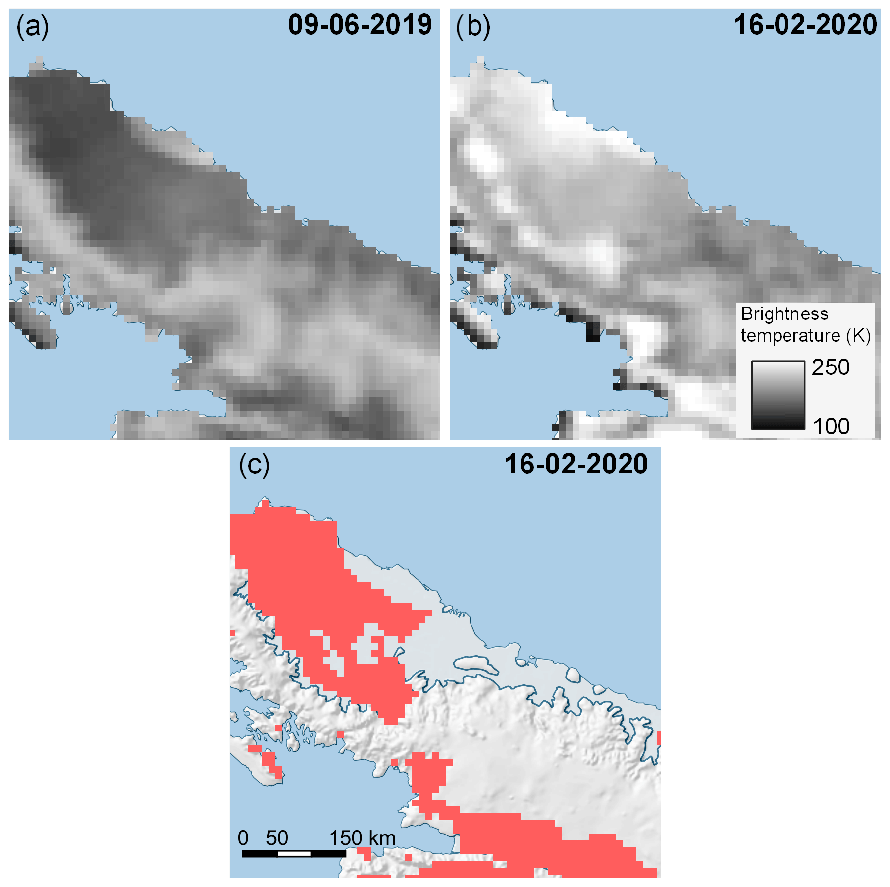
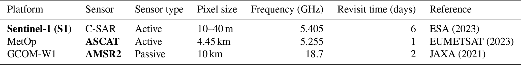
Figure 2Detection of wet snow in an AMSR2 image over the Antarctic Peninsula. (a) Brightness temperature (K) on 9 June 2019. (b) Brightness temperature (K) on 16 February 2020. (c) Pixels considered to contain wet snow after applying the wet-snow detection algorithm. The increase in brightness temperature between (a) and (b) is attributed to the presence of liquid water in the snowpack.
2.1.2 Sentinel-1 (S1)
One of the active sensor datasets is retrieved from the Sentinel-1 (S1) satellite constellation from the European Space Agency's (ESA) Copernicus space program. Starting with the launch of S1-A in 2014, the Sentinel-1 constellation gives access to data combining high spatial resolution and low revisit time covering most of the globe. With the synthetic aperture radar (SAR) technology, S1 products reach a spatial resolution on the order of tens of meters with a repeat pass of 6 d. By combining different orbital paths, it is possible to reduce the time between two observations of the same location to 2–3 d over the Antarctic Peninsula. Working in the C band (5.405 GHz), it is possible to detect the presence of liquid water in the snowpack in Sentinel-1 images by identifying changes in the backscattering coefficient σ0 through time (Johnson et al., 2020). With the increase in liquid water in the snowpack, comes a change in absorptivity and scattering mechanism (Nagler and Rott, 2000). These phenomena both lead to a decrease in σ0 (Moreira et al., 2013). As this coefficient changes little in Antarctica as long as the snowpack is dry, it is assumed that a significant change in backscattering is likely caused by the presence of water in the snowpack.
As for the passive sensors, several algorithms have been proposed to detect water in the snow with SAR and active sensors in general. Depending on the polarization, the frequency and the nature of the snowpack, the threshold applied to the backscattering values is variable (Koskinen et al., 1997; Nagler et al., 2016). For a C-band radar, a 3 dB decrease in σ0 has been employed as a threshold by Nagler and Rott (2000) and Johnson et al. (2020). In the present article, we used a −2.66 dB threshold after normalization of the images to their winter mean as the threshold to classify the snowpack as dry or wet. This threshold has been proposed by Liang et al. (2021) and was found to be effective for the Antarctic ice sheet.
To minimize the time between two Sentinel-1 acquisitions, all available images overlapping the study region were processed. To handle the large amount of data, image processing was carried out on Google Earth Engine (GEE, Gorelick et al., 2017). The S1 dataset available on GEE is already preprocessed following the implementation of the Sentinel-1 Toolbox from ESA (GEE, 2022; ESA, 2022). These processing operations include an update of the orbit metadata, removal of the low-intensity noise on the scene edges, a reduction in the discontinuities between sub-swaths, a radiometric calibration and a terrain correction using the ASTER digital elevation model. The choice has been made to resample S1 images from the original 10–40 m resolution to a 1 km resolution using mean values before detecting wet snow as data is ultimately interpolated onto the 7.5 km MAR grid. Before resampling, a 3×3 refined Lee speckle low-pass filter developed by Mullissa et al. (2021) was applied to the images in addition to a radiometric terrain flattening using the 1 arcmin global ETOPO1 DEM (Amante and Eakins, 2009). Pixels with values lower than −28 dB were removed from the dataset.
After resampling, the images are normalized to their austral winter mean. The winter mean is the average value of σ0 for each pixel, calculated using observations from June to October. To deal with changes in volumetric scattering related to the acquisition geometry, only the acquisitions from the same orbit overlapping by more than 95 % are taken into account to calculate the winter mean. Consequently, differences between the acquisitions are independent of the topography and the local context. The liquid water in the snowpack is then detected in the image by applying a −2.66 dB threshold (Fig. 3), following Liang et al. (2021).
To create daily wet-snow masks, Sentinel-1 images collected on the same day were combined. In the case where three or more images overlap, the snow state is selected by a majority filter, and the acquisition time is defined as the mean time between the selected acquisitions. In the case where there are only two images that contradict each other, a non-wet status is assumed. The acquisition time selected is the acquisition time of the non-wet image.
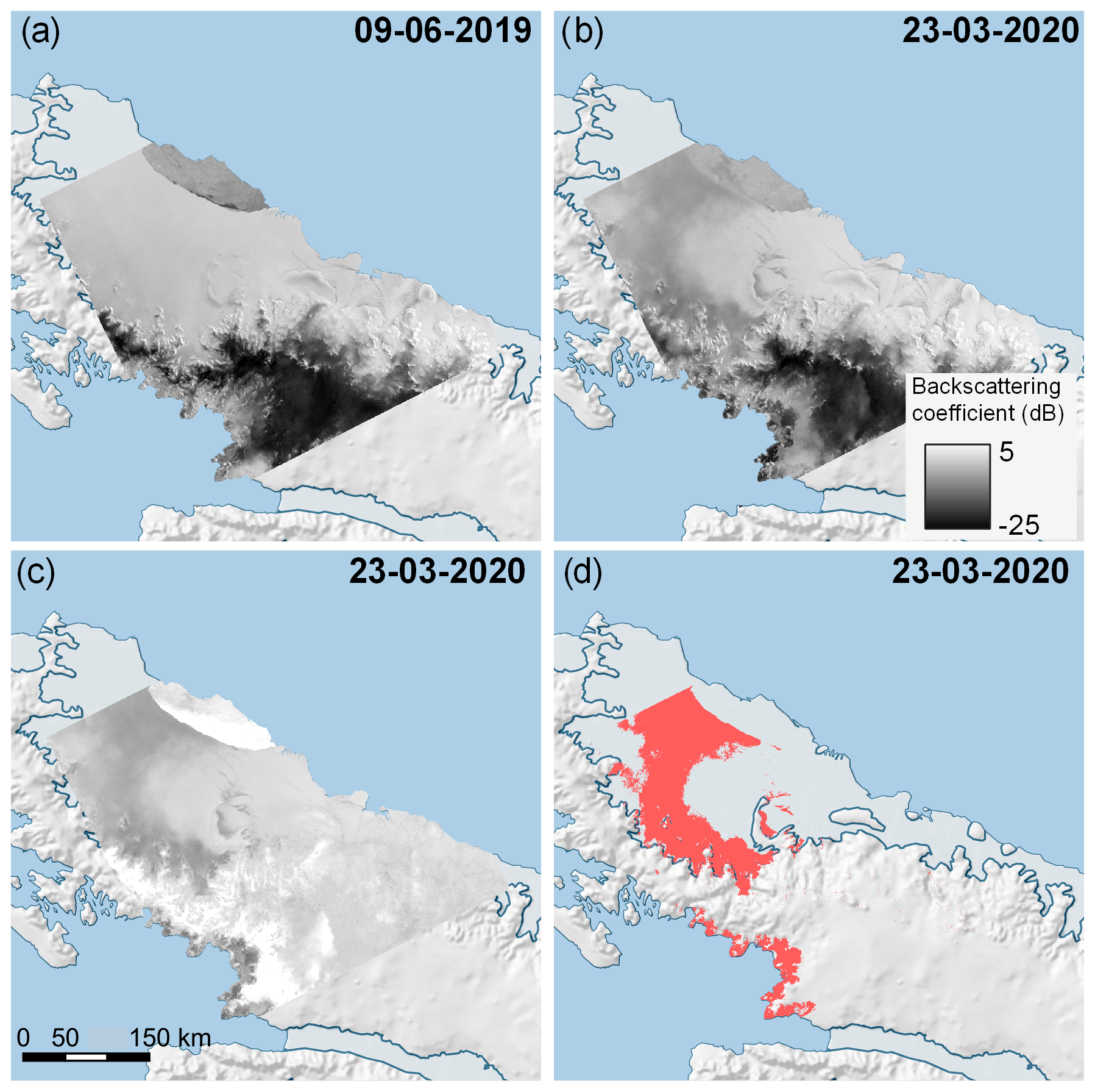
Figure 3Detection of wet snow in a Sentinel-1 image over the Antarctic Peninsula. (a) Backscattering coefficient σ0 (dB) on 9 June 2019. (b) Backscattering coefficient σ0 (dB) on 23 March 2020. (c) Normalized backscattering coefficient of 23 March 2020 relative to the winter mean. (d) Pixels considered to be wet snow after thresholding the normalized image. The decrease in backscatter between (a) and (b) is attributed to the presence of liquid water in the snowpack.
2.1.3 Advanced Scatterometer (ASCAT)
The third sensor we are using for this study is the C-band “Advanced Scatterometer” (ASCAT) aboard the MetOp satellites from the space segment of the EUMETSAT Polar System. ASCAT data are retrieved from the EUMETSAT data service portal (EUMETSAT, 2023). After resolution enhancement (Lindsley and Long, 2016), the product provides a backscattering coefficient σ0 at 4.45 km resolution by accumulating images over ∼2 d periods. In Antarctica, only morning passes are selected for this study. The detection of wet snow is performed using a simple thresholding technique (Ashcraft and Long, 2006), similar to the one used for Sentinel-1 images. The winter-mean backscattering coefficient is first calculated for each pixel and year from the observations from June–August. Then every measurement lower than this mean by 3 dB is considered wet snow. Similarly to AMSR2 daily products, the Sentinel-1 and ASCAT daily wet and dry images are interpolated onto the MAR grid.
In the end, from the three satellite datasets, four binary masks have been created. One from Sentinel-1, one from ASCAT and two from AMSR2, obtained by separating the ascending (evening) and the descending (morning) passes.
2.2 The regional climate model
For this study, we employed the MAR v3.12 RCM. MAR is a polar-oriented regional climate model mostly used to study both the Greenland (Delhasse et al., 2020; Fettweis et al., 2021) and Antarctic ice sheets (Glaude et al., 2020; Kittel et al., 2021). Its atmospheric dynamics are based on a hydrostatic approximation of primitive equations originally described in Gallée and Schayes (1994) and the radiative transfer scheme is adapted from Morcrette (2002). The transfer of mass and energy between the atmospheric part of the model and the soil is handled by the Soil Ice Snow Vegetation Atmospheric Transfer module (SISVAT, Ridder and Gallée, 1998), from which snow and snow and ice albedo sub-modules are based on the CROCUS snow model (Brun et al., 1992). The model has been parameterized to resolve the top 20 m of the snowpack, divided into 30 layers of time-varying thickness. MAR is configured with a decreasing vertical resolution of the snow layers from the top to the bottom. The maximum thickness of near-surface layers is on the centimeter scale, while below the first meter the maximum thickness is on the order of 1 m. The maximum layer thicknesses for the top four snow layers are 2, 5, 10, and 30 cm, respectively. Each layer has a maximum liquid water content (LWC) of 5 % of its air content beyond which the water freely percolates to deeper layers or runs off above impermeable layers (bare ice or ice lenses) (Coléou and Lesaffre, 1998).
Version 3.12 of MAR includes recent improvements in the snowpack temperature and the water mass conservation in the soil as described in Lambin et al. (2022). MAR was run at a 7.5 km resolution over the Antarctic Peninsula with a 40 s time step and with the spatial extent of the simulations corresponding to the extent of Fig. 1. It was forced at its lateral boundaries and over the ocean (sea surface temperature and sea ice cover) by the 6-hourly ERA5 reanalysis (Hersbach et al., 2020) between March 2017 and May 2021. The snowpack was initialized in March 2017 with a previous MAR simulation (Kittel et al., 2021). The blowing snow module of MAR is not used in this study, and snow drift is therefore not represented in the simulation.
2.3 Data assimilation
The satellite sensors are sensitive to the presence of liquid water into the snowpack rather than the physical process of melt. The aim of the data assimilation is therefore to guide or constrain the snowpack LWC of the model by nudging its temperature to induce melt or refreeze to match the observed surface state (Fig. 4).
The assimilation routine involves comparing, pixel by pixel, the modeled and the satellite wet-snow masks. The satellite wet-snow mask pixel is used for the assimilation if the indicated acquisition time is separated by less than 1.5 h from the time in MAR (1.5 h before and after the MAR time). The 3 h window enables the model to adapt its behavior but with limited short-term impact. As up to three satellite products are assimilated at the same time, three separate cases have been developed depending on the number of assimilated masks. Each case is called according to the number of acquisitions that are taken into account. However, a daily cycle in brightness temperature and thus in wet snow can exist over Antarctica (Picard and Fily, 2006). To take this into account, if there are three satellite observations available for a pixel for a single day, an observation of dry snow between two wet-snow observations is considered a false negative. Consequently, the corresponding dry-snow pixel is excluded for the day. For computational reasons, the assimilation routine is called at each MAR time step only during the melting season, between October and April. Outside of this time frame, no assimilation is performed due to computational constraints and the likely prevalence of shorter-duration melting events during winter. These events are commonly related to Foehn effects near the grounding line (Kuipers Munneke et al., 2018) where the effectiveness of passive sensors decreases.
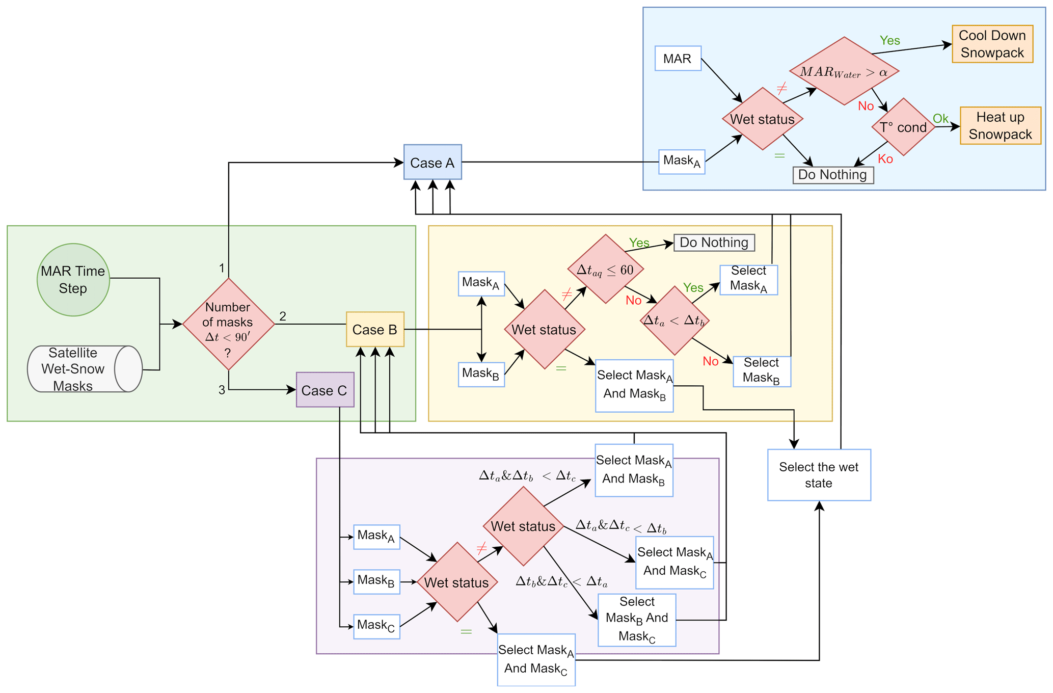
Figure 4Flowchart of the assimilation algorithm. The number of satellite images available around the MAR time step determines the subprocess that is called in the routine. The following three subprocesses are defined: case A, case B and case C. They represent the availability of 1, 2, and 3 wet-snow masks for assimilation, respectively. Cases B and C are funneled to case A so that no contradictory information is passed into MAR.
The first case of assimilation represents the situation where a single acquisition is available for a time step (case A in Fig. 4). It is the most frequent case applied (between 90 % and 95 % of the occurrence depending on the year). This case is inspired by the assimilation performed in Kittel et al. (2022). For the 3 h centered on the observation, at each MAR time step the quantity of liquid water modeled within the pixel is compared to the satellite-based wet-snow condition for the same pixel. If the modeled LWC of the snowpack is under a certain threshold (α) while the satellite mask indicates wet snow, the snow layers up to a certain depth (Δz) are heated by 0.15 ∘C if the snow layers are colder than 0 ∘C. In the opposite case, if the LWC is above the threshold α, but no wet snow is observed by satellites, the snowpack is cooled by the same amount of 0.15 ∘C. The process is applied at each MAR time step for which the conditions apply. However, two conditions prevent changes in the MAR snowpack temperature. The first is that if the snow density is above 830 kg m−3, the layer is considered to be ice and the model does not permit liquid water to accumulate within ice. The temperature in this case remains unchanged as the LWC threshold should never be reached. The second condition is the temperature of the snow layers above the depth Δz. If their mean temperature is below −7.5 ∘C, the MAR snowpack is too cold to be able to produce meltwater through warming, and the satellite observation is ignored. This operation is repeated at each time step for which MAR and observations disagree until the α threshold is reached or the observation is out of the time range. The choices for thresholds α and Δz are discussed in the two following sections, i.e., Sect. 2.3.1 and 2.3.2.
The second assimilation case (case B in Fig. 4) occurs when there are only two satellite observations within the 3 h window centered on the MAR time. If the two satellite-derived observations agree, MAR is adjusted according to the observed snow state as in case A but with a depth Δz equivalent to the mean values of the thresholds that would have been used for the individual satellite-derived masks. If the two observations indicate different snow states, a different processing is applied if the acquisitions are close to each other in time (within an hour) or not. For two inconsistent observations spread by more than 1 h, the assimilated snow state is the snow state from the closest image to the MAR time following the first case (case A). For two close contradictory observations, nothing is assimilated as they are considered both equally likely to be correct or incorrect. Valuable information may be lost in this case. For instance, the difference in penetration depth can cause a deeper-penetrating signal to observe liquid water (Fig. 5). However, as we have no additional information on the depth at which the water may be present, in this case the model is run as if there was no observation available.
The third case is when all three observations are available within the same 3 h time window (case C in Fig. 4). As for the second case, if the three observations agree with the same wet or non-wet snow status, they are considered as one and case A is called. Again, the depth Δz used is equivalent to the mean values of the thresholds that would have been used separately. If a single observation is different from the other two, the two closest observations to the MAR time are analyzed, applying case B described above. For our configuration of sensors, this third case is only encountered a couple of times (less than 1 % of all occurrences) while assimilating wet-snow masks of AMSR2 (ascending orbit), ASCAT and Sentinel-1.
2.3.1 Choice of water content threshold (α)
Estimating the quantity of liquid water in the snowpack with a single satellite acquisition is challenging. Despite numerous research studies, knowledge on the subject remains limited (Trusel et al., 2013; Fricker et al., 2021). However, as described in Picard et al. (2022), it is possible to find a typical LWC for which the satellite signal significantly changes and can be detected as melting or wet snow. Picard et al. (2022) demonstrates the capability of detecting small amounts of water using the radio frequencies employed in this study. Only 0.11 and 0.05 kg m−2 of liquid water is necessary at 6 and 19 GHz, respectively, if the water is uniformly spread over the pixel. This quantity can be higher for heterogeneous pixels containing dry or wet patches. For this study, the choice has been made to use the same threshold regardless of the sensor frequency. AMSR2 acquires data at higher frequencies and is theoretically more sensitive, but it has a coarser resolution than the two active sensors. Its pixels tend to be more heterogeneous, suggesting a compensation with regard to liquid water quantity. Two different thresholds are tested to study the sensitivity of the model. Both have been shown to significantly change the snowpack brightness temperature in the literature. Tedesco et al. (2007) proposed a LWC threshold of 0.2 %, while Picard et al. (2022) proposed a threshold of 0.1 % of the snowpack mass. They have both been tested in Kittel et al. (2022) where the choice between the two was found not to significantly influence the melt quantity produced by the MAR model. The sensitivity of the microwave sensors is high enough that the quantities of liquid water that can be detected are much smaller than that produced during a typical melting day (1.2±0.6 % as modeled by MAR over the studied zone in the top meter of snow). Currently, there is no means of identifying the best-fitting threshold for this study.
2.3.2 Choice of assimilation depth threshold (Δz)
Microwaves have penetration capabilities directly related to their wavelength (Elachi and van Zyl, 2006). As a consequence, the C band from Sentinel-1 and ASCAT has a different penetration depth than Ku band from AMSR2. In addition, the water content strongly influences the penetration depth, as water at the top of the snowpack can prevent deeper penetration (Fig. 5). In this experiment, we set different penetration depths for each remote-sensing product to test its influence. Using AMSR2 (Ku band), we consider an assimilation depth Δz=0.1, 0.2 and 0.4 m successively below the surface. Below this depth, the electromagnetic wave should not have a noticeable influence (Picard et al., 2022). For Sentinel-1 and ASCAT (C band), the depth thresholds Δz are set to 0.5, 1, and 1.5 m, as the signal is expected to penetrate deeper into the snowpack.
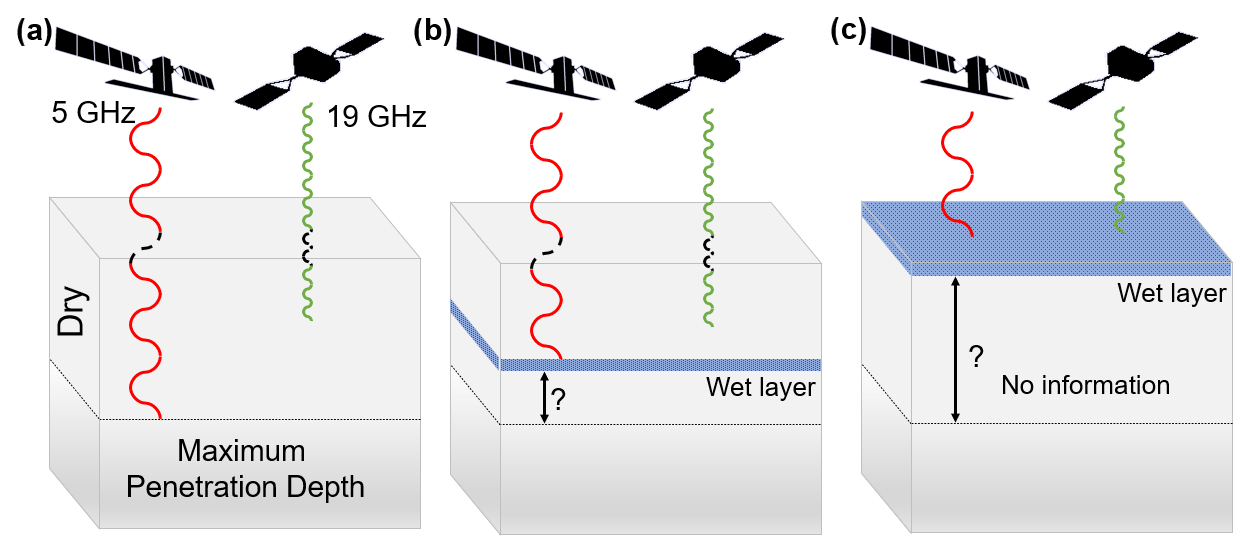
Figure 5Illustration of the penetration depth of the microwave sensors according to their wavelength and the depth of the wet snow layer. (a) Penetration depth in a dry snowpack. The signal of the sensor with the lower frequency (5 GHz, in red) penetrates deeper than the signal of the higher-frequency sensor (19 GHz, in green). (b) Penetration depth with a layer of liquid water deep in the snowpack. The microwave sensor with deeper penetration can detect water presence, but the other cannot. (c) Penetration depth with liquid water at the top of the snowpack. Both satellites can observe the presence of liquid water.
2.3.3 Experiments conducted
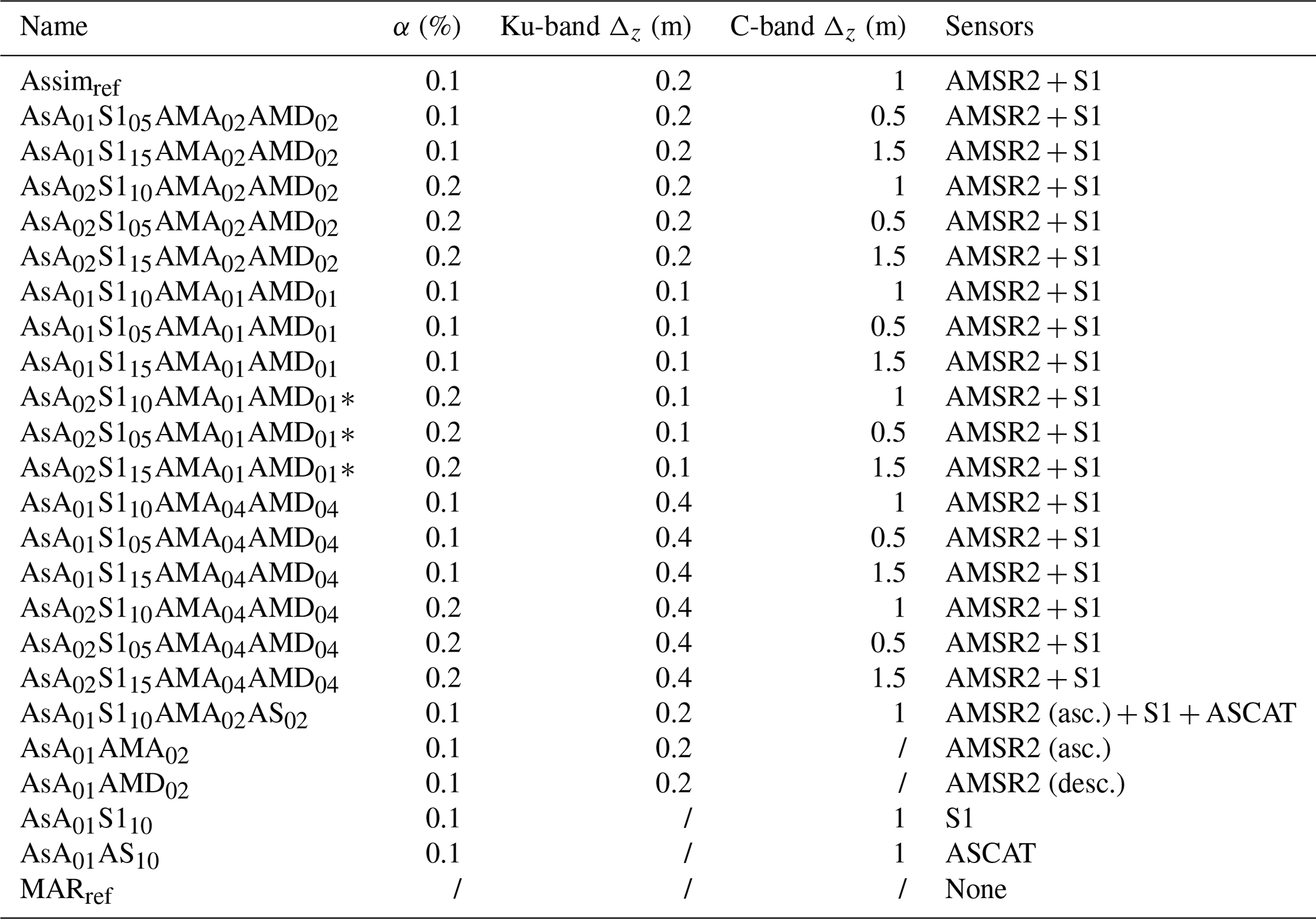
An ensemble of 24 MAR simulations is presented here. Only the reference MAR simulation, MARref, is performed without assimilation. The others are referred to as “assimilations” hereafter. Their naming convention is “As” followed by “A” and the value of the α threshold in the subscript (in %), the remote sensing (RS) datasets assimilated, and their corresponding Δz threshold value in the subscript (in m). “S1” refers to the S1 dataset, “AMA” to AMSR2 ascending, “AMD” to AMSR2 descending, and “AS” to ASCAT. The assimilations were started in January 2019 and have been initialized from the simulation without assimilation (which begins in 2017). For each assimilation, the satellite wet-snow masks are assimilated into the model, with different parameters for the α threshold and C-band and Ku-band Δz thresholds (Table 2). The reference assimilation (Assimref) is performed using Sentinel-1 and AMSR2, with both their ascending and descending orbits, and with assimilation depth thresholds Δz=1 and 0.2 m, respectively. In addition, the liquid water content threshold α is set at 0.1 %. The thresholds used to perform Assimref correspond to values given in the literature (Elachi and van Zyl, 2006; Picard et al., 2022). The other assimilated simulations have been performed with a combination of three satellite products chosen between Sentinel-1, AMSR2 ascending, AMSR2 descending and ASCAT and with a combination of the assimilation parameters. The assimilations have been performed for the periods June 2019 to May 2020 and June 2020 to May 2021. The present document focuses on the 2019–2020 melt season, while figures for the 2020–2021 season are available in the Supplement.
Table 2The different simulations performed in this study, including data assimilation parameters. When not specified, both ascending and descending paths of AMSR2 are assimilated. Simulations marked with an asterisk and those with assimilation of only one sensor are not taken into account in the calculation of the ensemble average.
Because the integrated physics within RCMs is either partially resolved or contains uncertainties, it is first required to evaluate model outputs against in situ measurements. The evaluation is performed in order to quantify how close the model is to reality and to determine if the model is inclined to reproduce the observations. Since our focus is on assessing the model sensitivity through assimilation, we exclusively evaluate MAR without assimilation. It is worth noting that the values derived from the assimilations may diverge from the observations due to the assimilation algorithm sensitivity rather than the model physics.
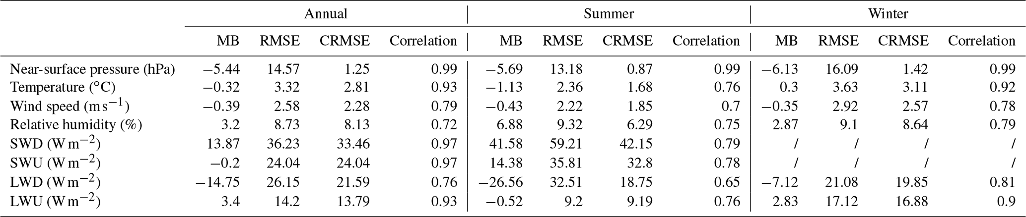
The outputs of the model simulation without assimilation are evaluated by comparing with in situ observations. The daily observations are provided by automatic weather stations (AWSs) spread across the AIS. Here, nine AWS datasets available in the study area (blue crosses displayed in Fig. 1) have been gathered to calculate statistics for the model vs. the observations as done in Kittel (2021) and Mottram et al. (2021). The statistics employed for the evaluation are the mean bias (MB), root-mean-square error (RMSE), centered root-mean-square error (CRMSE) and correlation coefficient (r) (Table 3). The statistics are listed for the 2016–2021 period for the near-surface pressure, temperature, wind speed, relative humidity and modeled energy balance components, including shortwave downward radiation (SWD), shortwave upward radiation (SWU), longwave downward radiation (LWD) and longwave upward radiation (LWU).
Small biases can occur in the comparison as a result of the elevation difference between the in situ observations and the model. The AWS observations are point measurements, whereas the model provides information over a 7.5×7.5 km2 pixel. Thus, the mean elevation of the MAR pixel in which the AWS falls is not the same as the AWS true elevation. This difference is particularly noticeable for the near-surface pressure, which is directly linked to the elevation. Nonetheless, a high correlation (r>0.98) reflects the ability of MAR to simulate the observed temporal variability.
In general, the winter season is slightly better represented by MAR with higher correlations and lower mean bias than the summer season. A weaker correlation is observed in summer for longwave downward radiation (r=0.65). This difference is compensated for by an overestimation of shortwave downward solar radiation in summer. MAR does not assimilate observed temperature profiles or coastal temperatures but is forced at its lateral boundaries and at the sea surface every 6 h with temperature, specific humidity, wind and sea surface temperature. Thus, modeled clouds are strongly influenced by the internal model climate and microphysics (Delhasse et al., 2020). Moreover, the radiative scheme implemented in MAR is the scheme employed by the ERA-40 reanalysis. This scheme has been updated in the ERA-5 reanalysis (Hersbach et al., 2020) but not in MAR. MAR also tends to underestimate the liquid water path during summer when compared to Cloudsat and CALIPSO estimates described in Van Tricht et al. (2016). This underestimation is partially responsible for the LWD bias in summer.
Table 3Mean bias (MB), root-mean-square error (RMSE), centered root-mean-square error (CRMSE), and correlation between MAR and daily observations over the Antarctic Peninsula. A negative value implies a lower MAR estimate compared to the observation. Statistics are given for the near-surface pressure, temperature, wind speed, relative humidity, shortwave downward radiation (SWD), shortwave upward radiation (SWU), longwave downward radiation (LWD), and longwave upward radiation (LWU) radiation annually and for the summer (DJF) and winter (JJA) seasons and are calculated for the 2016–2021 period. During winter, incoming solar radiation is absent, and therefore shortwave solar radiation estimates (SWD and SWU) are not provided. Locations of the weather stations used for the daily observations are marked by blue crosses in Fig. 1.
In addition, Jakobs et al. (2020) provide melt estimates from the AWS that can be compared to the surface melt production of the four closest MAR pixels to the AWS (Fig. 6). MAR tends to overestimate some extremes in meltwater production but also tends to underestimate melt during low-melt seasons. There are also differences in the length of the melt season, with MAR sometimes overestimating and sometimes underestimating the duration of the season. Although the difference in altitude between the AWS and MAR pixels may explain some of the differences between the two datasets, these discrepancies also highlight the importance of nudging MAR to better reproduce the remote sensing observations of the snowpack state.
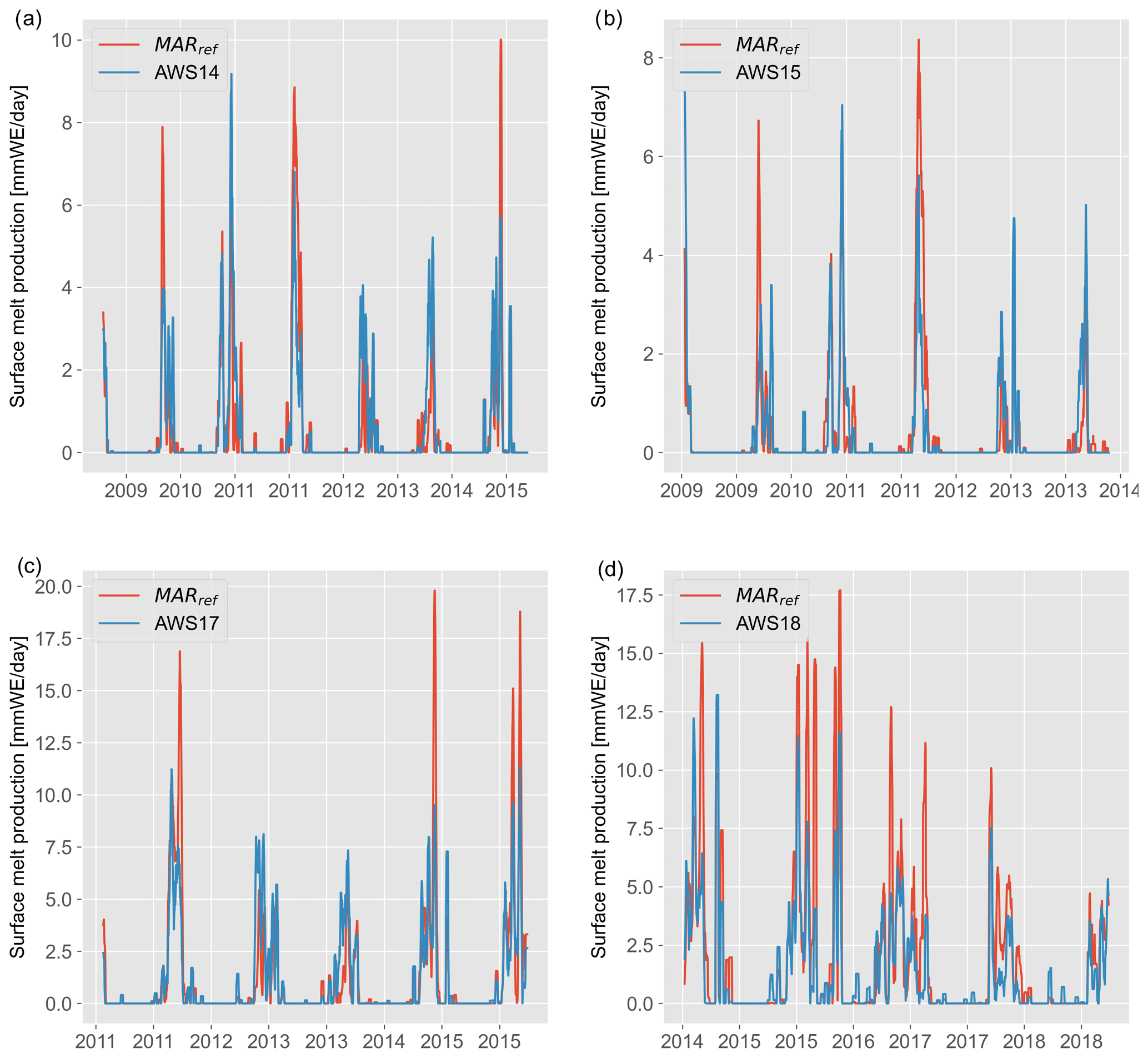
Figure 6Comparison of surface meltwater production (mm WE d−1) as modeled by MARref (in red) and estimated surface meltwater production from AWS stations (a) 14, (b) 15, (c) 17 and (d) 18 (in blue) as described in Jakobs et al. (2020).
Table 4 provides a comprehensive summary of the results obtained from the 24 MAR simulations. The summary includes the number of melt days (i.e., the number of days where melt is occurring over at least 10 % of the ice sheet and ice shelves of the study area), surface melt (ME), runoff (RU), refreezing (RZ) and the surface mass balance (SMB). This table offers a concise overview of the simulation results. We analyzed the evolution of several variables in order to assess the sensitivity of the MAR model to the assimilation, including ME, RU, SMB, snowpack density (ρ) and liquid water content (LWC) (Table 5).The first three variables (ME, RU and SMB) are provided for the entire snowpack profile, while ρ and LWC are provided for the first meter. The average value of the variables across all assimilations, , is compared to the model simulation without assimilation (MARref). Three simulations have been discarded to calculate because of an unrealistic freeze–thaw cycle induced by the assimilation. These simulations are marked with an asterisk in Tables 2 and 4. So as not to incorporate bias from a single wet-snow mask, simulations assimilating only one wet-snow mask are also omitted in the calculation of .
Table 4Summary of the results of the different experiments conducted for the study. The number of melt days, cumulated surface meltwater, runoff, refreeze and surface mass balance over the 2019–2020 melt season are provided for each experiment for the entire MAR spatial extent, excluding ocean areas.
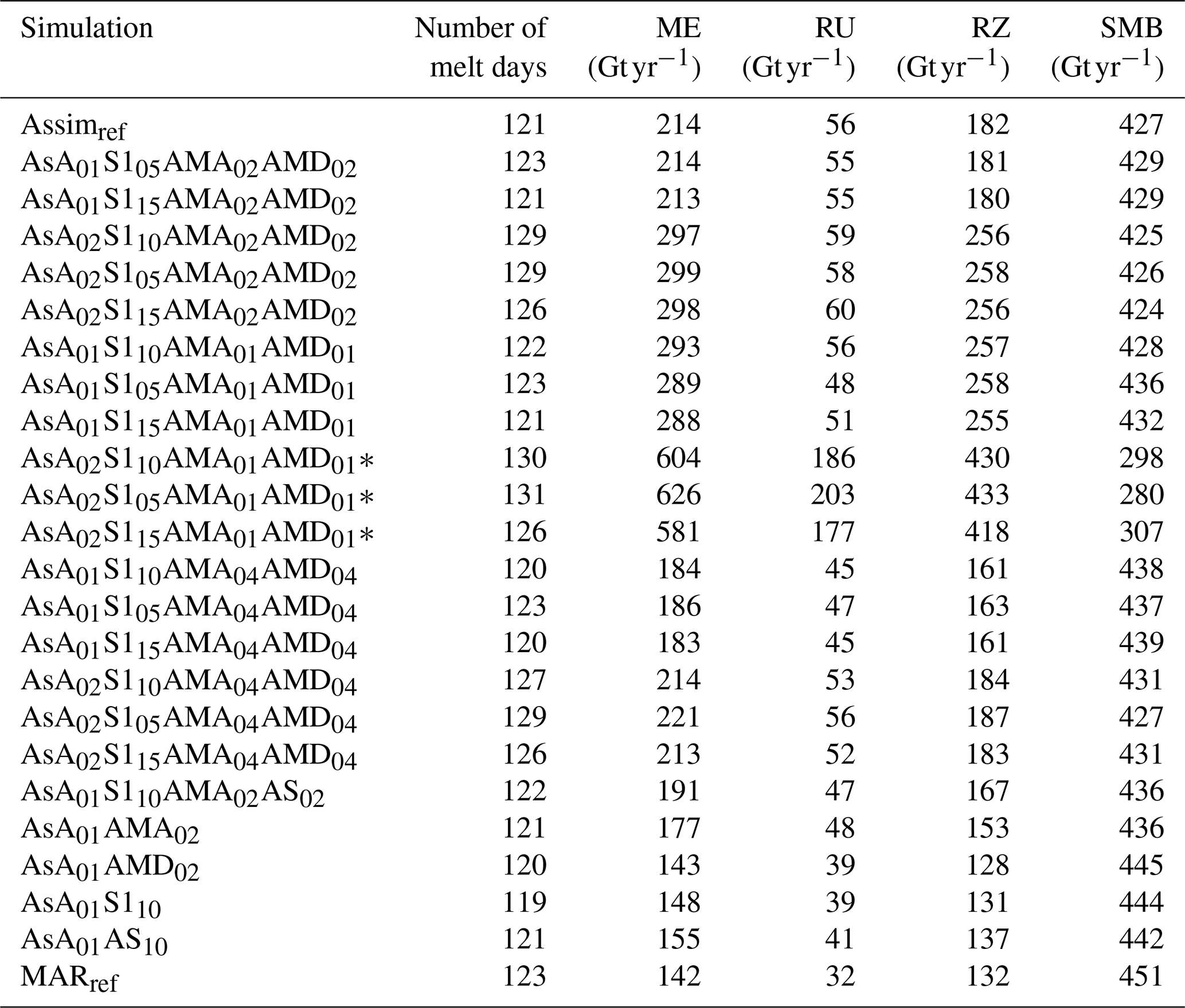
Table 5Difference (in Gt yr−1 and %) in surface meltwater production (ME), runoff (RU), refreezing (RZ), surface mass balance (SMB), snowpack liquid water content (LWC) and snowpack density (ρ) between MARref and the mean value of the assimilations () for 2019–2020 for the entire MAR spatial extent (including grounded ice and ice shelves). Variables are accumulated annually and over summer (November through April) except for snowpack density and the liquid water content, which are averaged over the periods. LWC and ρ are the average within the first meter of the snowpack, while the other variables are the total for the entire snowpack.
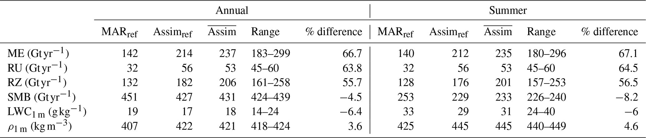
On average, the wet-snow extent provided by the wet-snow masks is larger than the extent modeled by MARref on the Antarctic Peninsula. This difference impacts the meltwater production in the model. Regardless of the parameterization used for the assimilation, the surface meltwater production is increased compared to MARref (Table 5), leading to a cumulative meltwater production increase of 66.7 % for over the year.
Meltwater that is produced within the snowpack will eventually either refreeze or run off, depending on the saturation level and thermal condition of the snowpack. The snowpack can saturate, either from excess meltwater production or from densification. If the MAR snowpack LWC exceeds 5 % of the firn air content (the irreducible water saturation), the excess water starts to percolate to deeper layers and run off. The evolution of runoff is thus directly related to the evolution of melt and the snowpack saturation level (Fig. 7). Therefore, the relative increase in surface melt for relative to MARref (67.7 %) is similar to the relative increase in runoff (63.8 %), but their absolute increase in Gt yr−1 is different (+95 and +21 Gt yr−1, respectively).
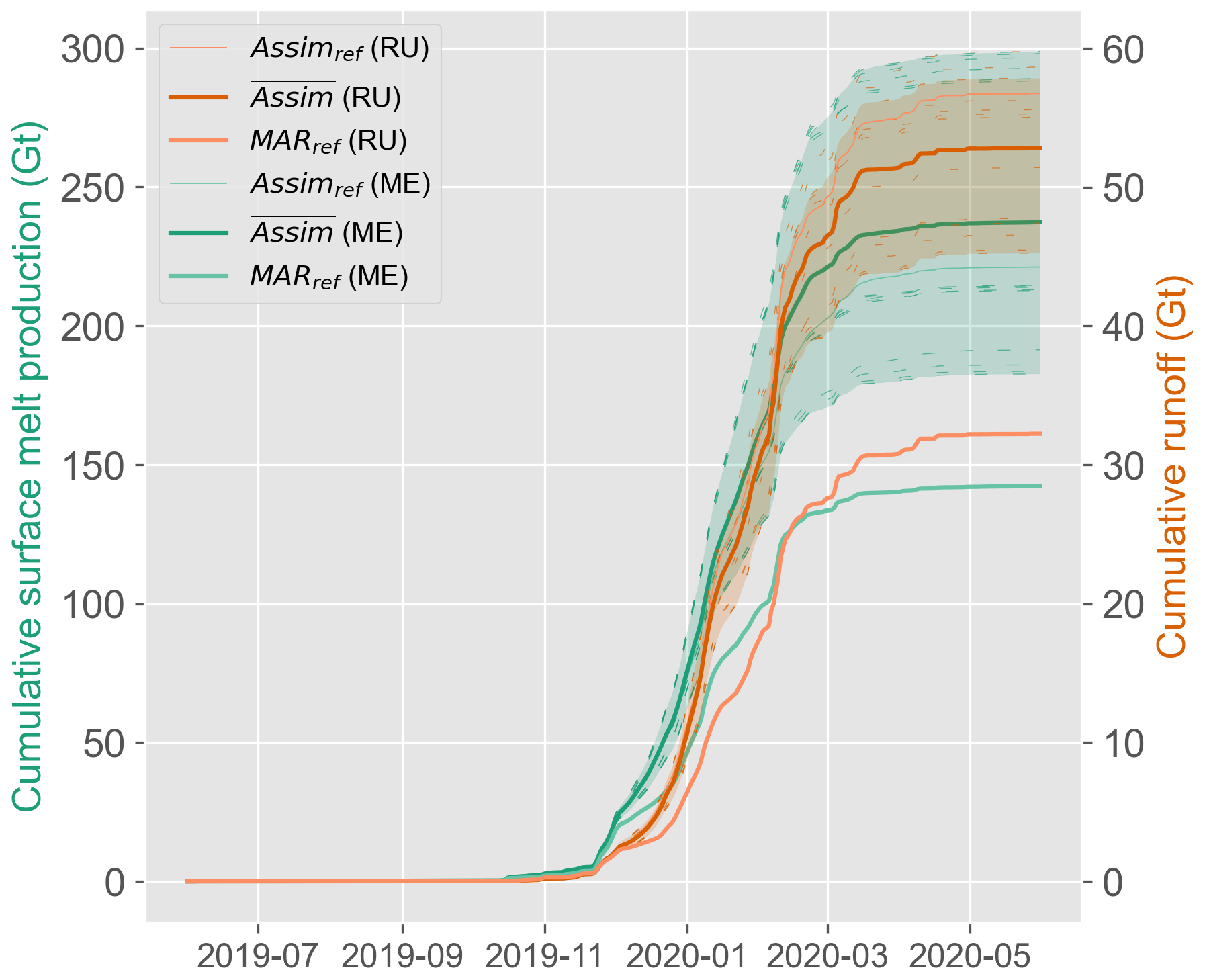
Figure 7Comparison between the cumulative surface meltwater production (Gt) in green and the cumulative runoff (Gt) in orange over the whole MAR domain (excluding ocean areas) for the 2019–2020 melt season as modeled by MAR without assimilation and with data assimilation. Shaded areas represent the range of the assimilations. While the increase (in Gt) is larger for meltwater production, the relative increase is similar for meltwater production and runoff.
The difference between the increase in meltwater production and the increase in runoff corresponds to an increase in refreezing, with a similar percentage change over the entire domain. This suggests that the snowpack can still absorb liquid water and convert it into refrozen ice in our simulations unless it reaches its maximum LWC. However, as discussed further below, the strongest increase in runoff occurs together with firn air content depletion over the ice shelves. In this case refreezing is large enough to substantially deplete the firn air content, leaving less storage space for liquid water in the perennial snowpack (Banwell et al., 2021).
As can be seen in Fig. 8, the data assimilation only has a slight effect on the overall SMB. The SMB expression is defined as the sum of the ablation terms (runoff, evaporation and sublimation) and accumulation terms (snowfall and rainfall). The cumulative SMB for the 2019–2020 melt season is only decreased by 4.5 % compared to the model without assimilation. The general trend in SMB remains positive within the study area. Only the ice shelves show negative SMB during austral summer (Fig. 9).
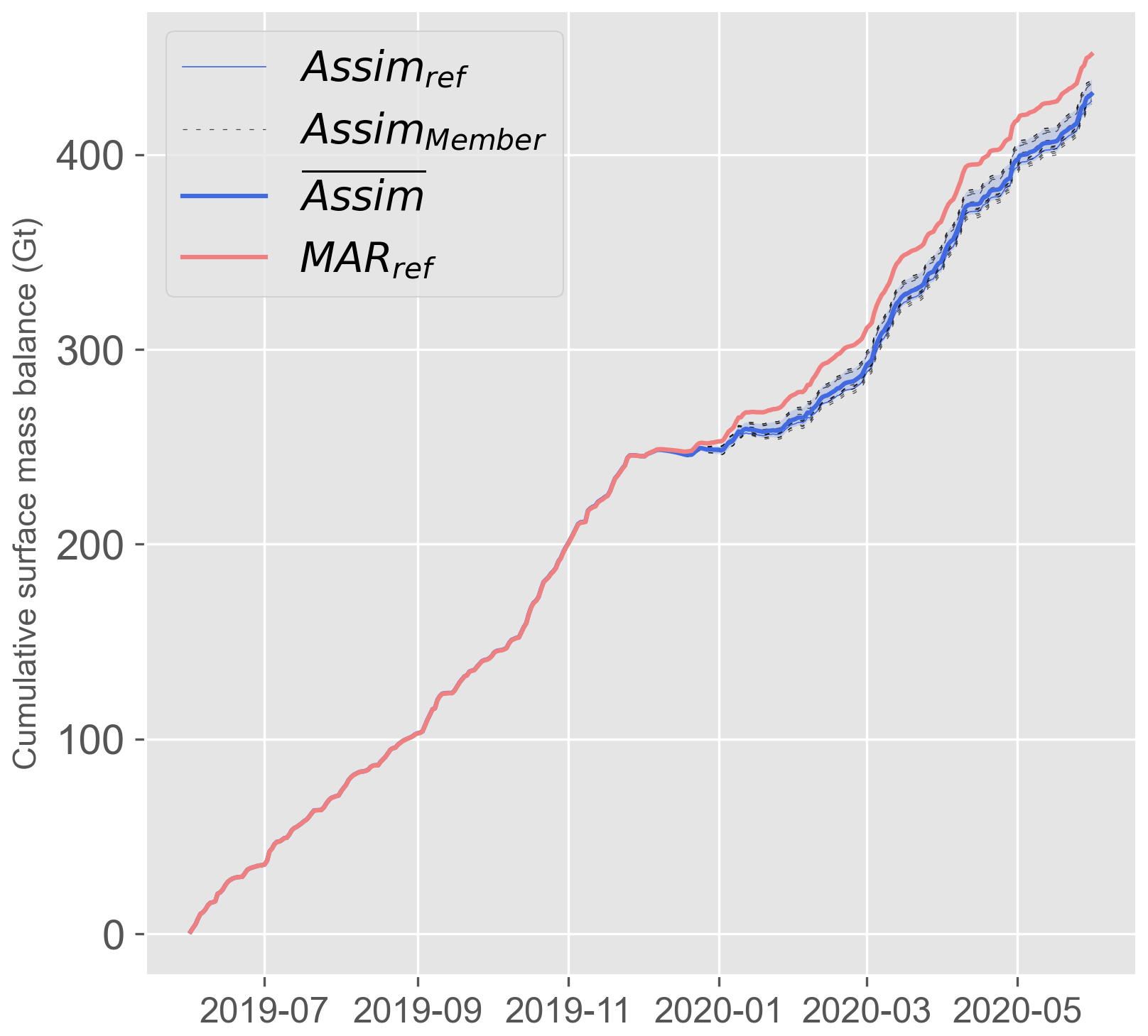
Figure 8Cumulative surface mass balance (Gt) over the entire MAR domain (excluding ocean areas) for the 2019–2020 melt season as modeled by MAR without assimilation (MARref in red), with data assimilation (Assimmember in dashed lines) and as an averaged value ( in blue). Shaded areas represent the range of the assimilations. Despite the increase in surface melt production, the surface mass balance does not significantly decrease.
The density and LWC of the snowpack are also impacted by the assimilation. As can be seen in Table 6, densification affects the LWC on the ice shelves where most of the surface melt and refreezing occurs. With a denser snowpack, firn air content is reduced, and there is less space for liquid water to be absorbed. Therefore, despite the increase in surface melt production, the assimilation process eventually leads to a decrease in the amount of liquid water retained in the snowpack. This reduction occurs due to the assimilations' impact on water retention capabilities of the snowpack through increased refreezing.
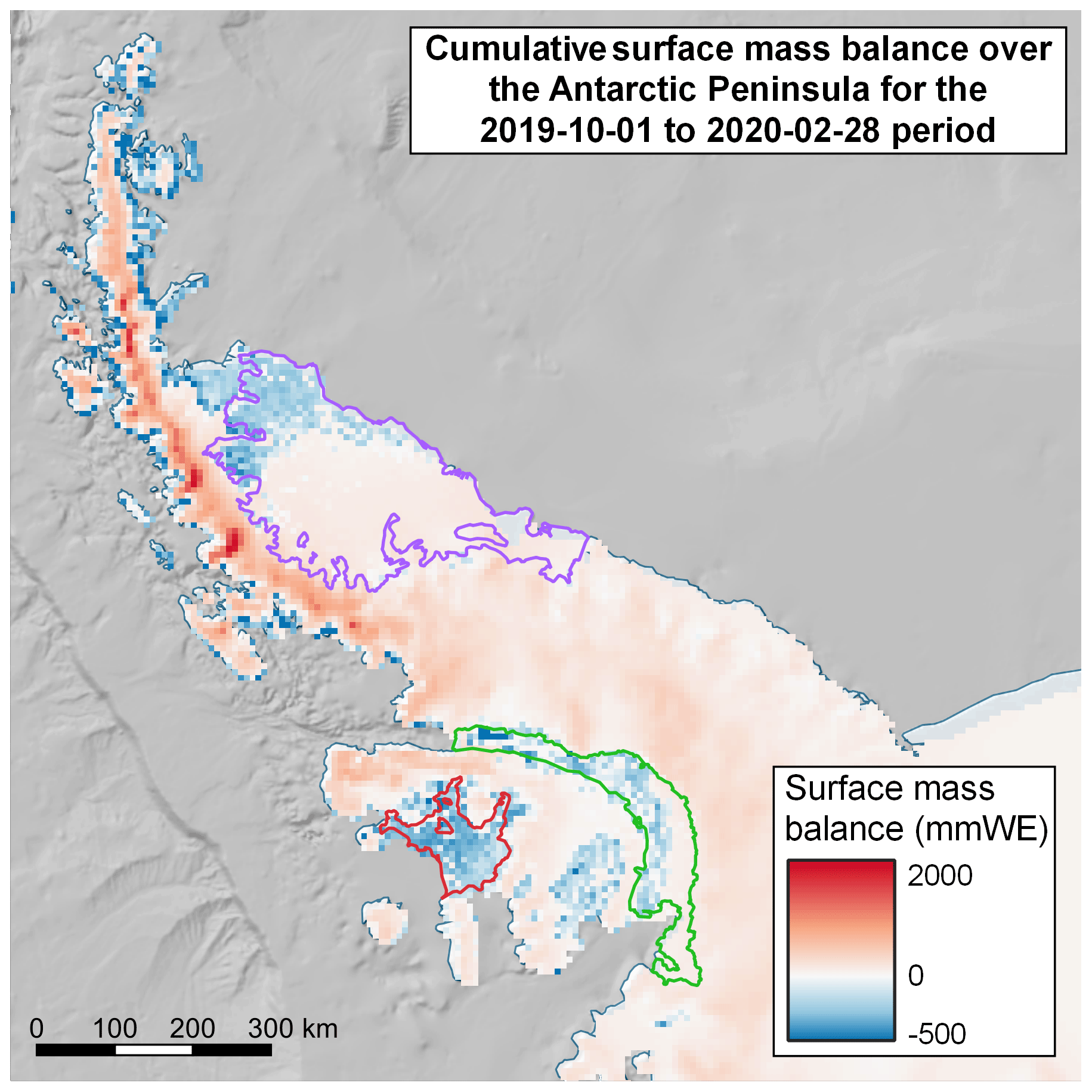
Figure 9Cumulative SMB (mm WE) from 1 October 2019 to 28 February 2020 over the AP as modeled by Assimref. Larsen C is outlined in purple, George VI in green and Wilkins in red. The southern ice shelves and the northernmost coastlines are experiencing a negative SMB in contrast with the rest of the AP. Larsen C is divided into two regimes. Its northern part is experiencing a negative SMB, while the southern part is positive.
All three highlighted ice shelves (Larsen C, Wilkins and George VI) experience an increase in surface melt, refreeze and runoff as a result of the assimilation (Table 6). On the Larsen C and Wilkins ice shelves, the percentage increase in runoff strongly outweighs the percentage increase in surface melt production. For Larsen C, the ice shelf experiencing increase in melt in absolute and relative terms (+21 Gt yr−1, i.e., +85.7 %), runoff triples (+6 Gt yr−1, i.e., +311.2 %). However, over the year its liquid water content only slightly increases (+1 %). It therefore appears that on ice shelves the increase in refreezing is not strong enough to compensate for the increase in melting. The depletion of firn air content leads to a swift saturation of the snowpack, producing a surplus of meltwater that results in a more pronounced decrease in SMB compared to other regions of the Antarctic Peninsula.
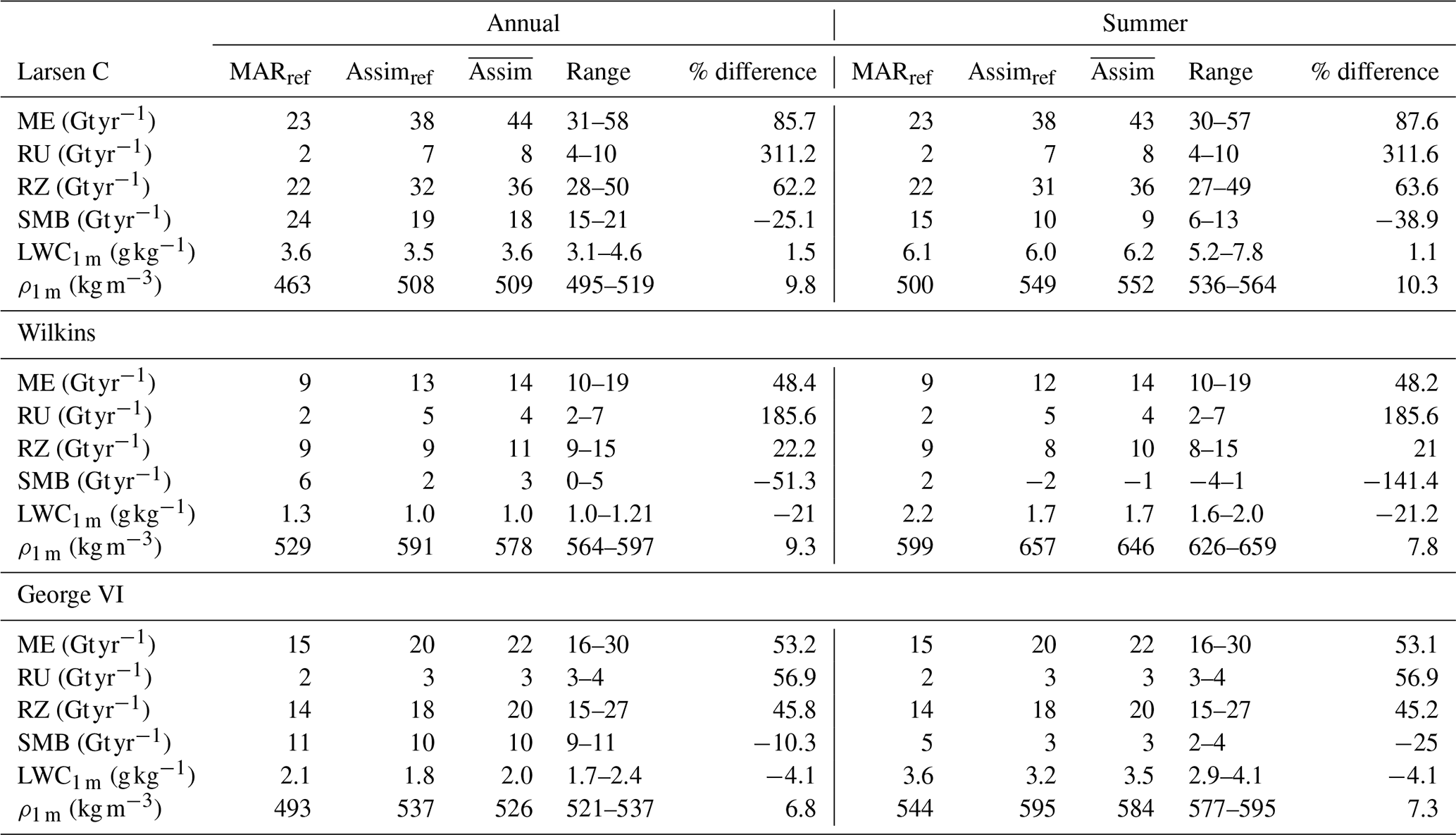
Table 6Difference (in Gt yr−1 and %) in surface melt production (ME), runoff (RU), refreezing (RZ), surface mass balance (SMB), snowpack liquid water content (LWC) and snowpack density (ρ) between MARref and the mean value of the assimilations () over the three highlighted ice shelves in 2019–2020 using the regions shown in Fig. 1. Variables are accumulated annually and over summer (November through April), except for snowpack density and the liquid water content, which are averages over the specified periods. LWC and ρ are given as the average of the snowpack first meter, while the other variables are totals for the entire modeled snowpack.
Except for the LWC, which remains relatively small and stable as it has been averaged over the season, the analyzed variables (ME, RU, RZ, SMB and snowpack density) have undergone noticeable variation as a result of the assimilation, causing MARref variables to always be outside of range of the assimilated simulations. The amplified surface melt production leads to concurrent effects, including increased runoff, reduced surface mass balance, and an increased occurrence of refreezing. This increase in runoff is attributed to the increase in melt combined with the densification of the upper layers of the snowpack, reducing its capacity to absorb meltwater.
In the end, the results illustrate that, on average, Assimref is the assimilation that gives the closest results to , making it an appropriate candidate in the case of limited computational resources (allowing for 1 simulation instead of 24). The parameters used in Assimref seem to be an appropriate option given the results presented below regarding sensitivity to the assimilation parameters.
4.1 MAR sensitivity
4.1.1 Sensitivity to the assimilation depth threshold
The assimilation depth used for low-penetrating sensors influences MAR meltwater production by inducing firn air content depletion. Due to refreezing, the uppermost portion of the snowpack becomes denser. The refreezing is accentuated when using a shallow-depth threshold (for example, 10 cm with AMSR2) as the top layers of the snowpack will contain the majority of the liquid water. Consequently, the increase in meltwater production needed to reach the α threshold (0.1 % or 0.2 %) will be greater (because of the denser snowpack) than for a deeper assimilation depth where less densification occurs. Also, with firn air content depletion, two other phenomena enhance melt production. First, the available energy in the system is consumed by the melting process, preventing layers below 1 m from heating up and reducing the release of latent heat from the refreezing process. Therefore, the deeper layers will tend to cool the snowpack, necessitating more nudging. The second phenomena is that during melt events the upper layers saturate with less water due to the densification. The saturation results in increased runoff and faster percolation of the water into deeper layers outside of the assimilation depth range. If the model were to retain liquid water in its top snow layers for a longer duration, it would require less nudging to match the RS datasets. This effect could be achieved by increasing the maximum liquid water content of the snow layers. However, enhancing water retention in the near-surface snowpack layers might lead to increased refreezing and consequently densification depending on the snowpack temperature (Fettweis et al., 2011).
This phenomenon is illustrated in Fig. 10, where using a 10 cm assimilation depth threshold for AMSR2 produces more melt than the 20 and 40 cm thresholds for water content thresholds of both 0.1 % and 0.2 %. The effect ends up being so important that using a 10 cm assimilation depth and 0.2 % α threshold for AMSR2 can result in an intense refreezing and firn air content depletion that leads to a strong increase in runoff, reducing SMB for the Antarctic Peninsula. This decrease in SMB is contrary to the generally observed trend (Rignot et al., 2019; Chuter et al., 2022). Consequently, the three simulations that use these parameters for the Ku-band sensors have been discarded in the computation of the average melt for the assimilations.
In contrast, with Sentinel-1, the effect of choosing different Δz thresholds is less pronounced. As shown in Table 4, assimilations that have all parameters in common except the S1 assimilation depth threshold only vary slightly (a few Gt yr−1) for all variables. Multiple reasons can explain this comparatively lighter effect. S1 has a larger revisit time compared to AMSR2 (a 6 d revisit time vs. daily images). With fewer images, the assimilation depth for S1 is used less frequently in the melt assimilation process within MAR. In addition, as explained previously, the liquid water is kept longer in these slightly deeper layers due to a higher retention capacity, and thus less melt is required to reach the water content threshold. Overall, these results indicate that MAR is more sensitive to a shallower assimilation depth threshold. Most of the sensitivity is linked to refreeze and densification, more likely to occur in the first centimeter of the snowpack. The penetration depth for the C-band sensors is larger than for Ku-band sensors, and using sensors with higher frequencies increases the sensitivity to the choice of the thresholds.
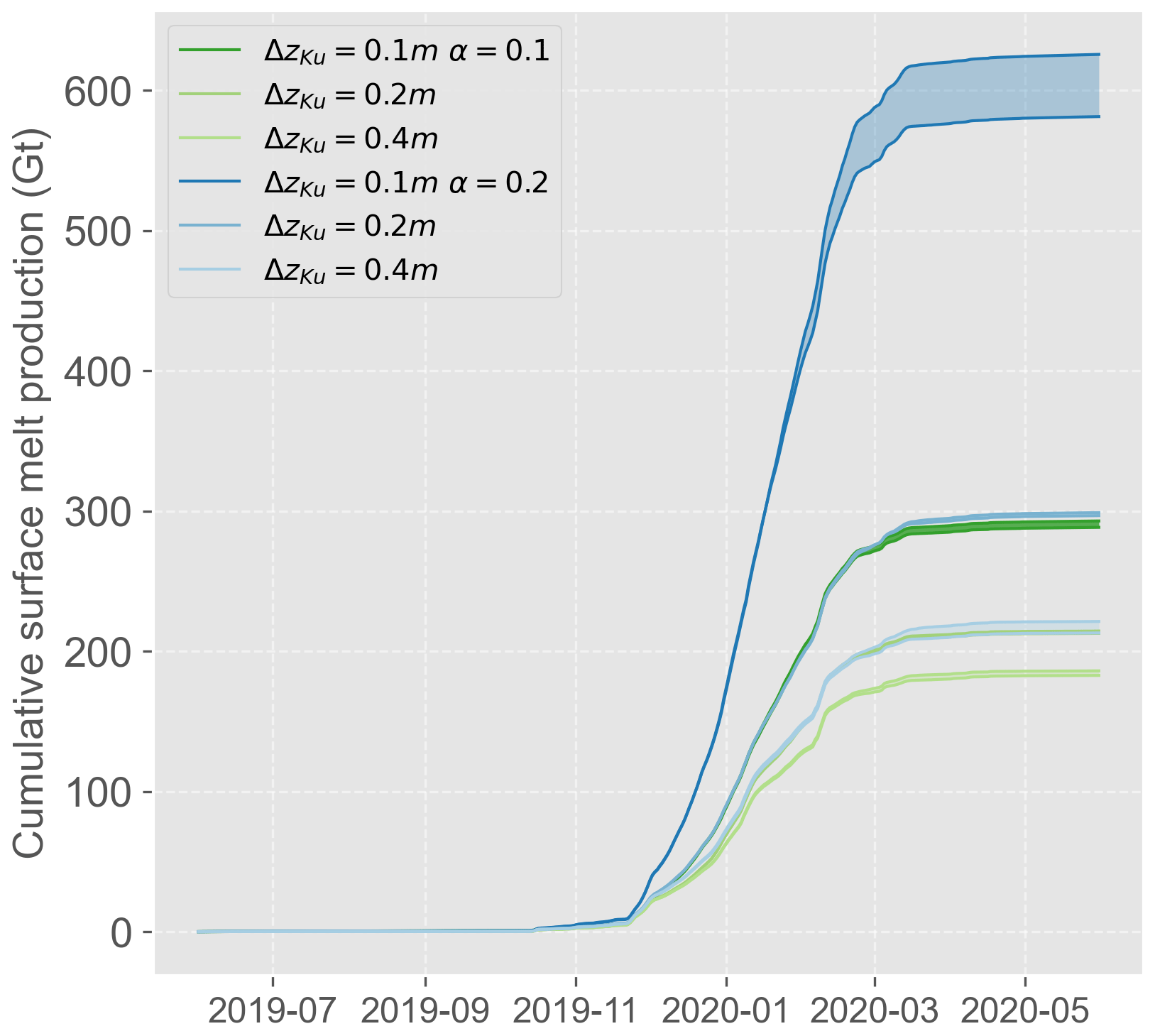
Figure 10Cumulative surface melt production (Gt) over the entire MAR domain for the 2019–2020 melt season as modeled by the different assimilation experiments. The assimilations are grouped by their α and Ku-band Δz thresholds. Shaded areas represent the range of the assimilation of the groups. Groups of assimilations with Ku-band Δz=0.1 m produce more melt than the group of assimilations with the same α but different Δz.
4.1.2 Sensitivity to the water content threshold
Experiments with varying the liquid water content threshold have a smaller impact compared to the assimilation depth experiments. Varying liquid water content influences the number of melt days modeled, thus expanding the melt season duration (Table 7) rather than the quantity of liquid water produced by melting. The amount of liquid water required to reach the water content thresholds α is small compared to the modeled LWC of a typical melt day. In MARref, for the 2019–2020 melt season, the value reaches 1.2 % for a melt day on average, above the 0.2 % threshold.
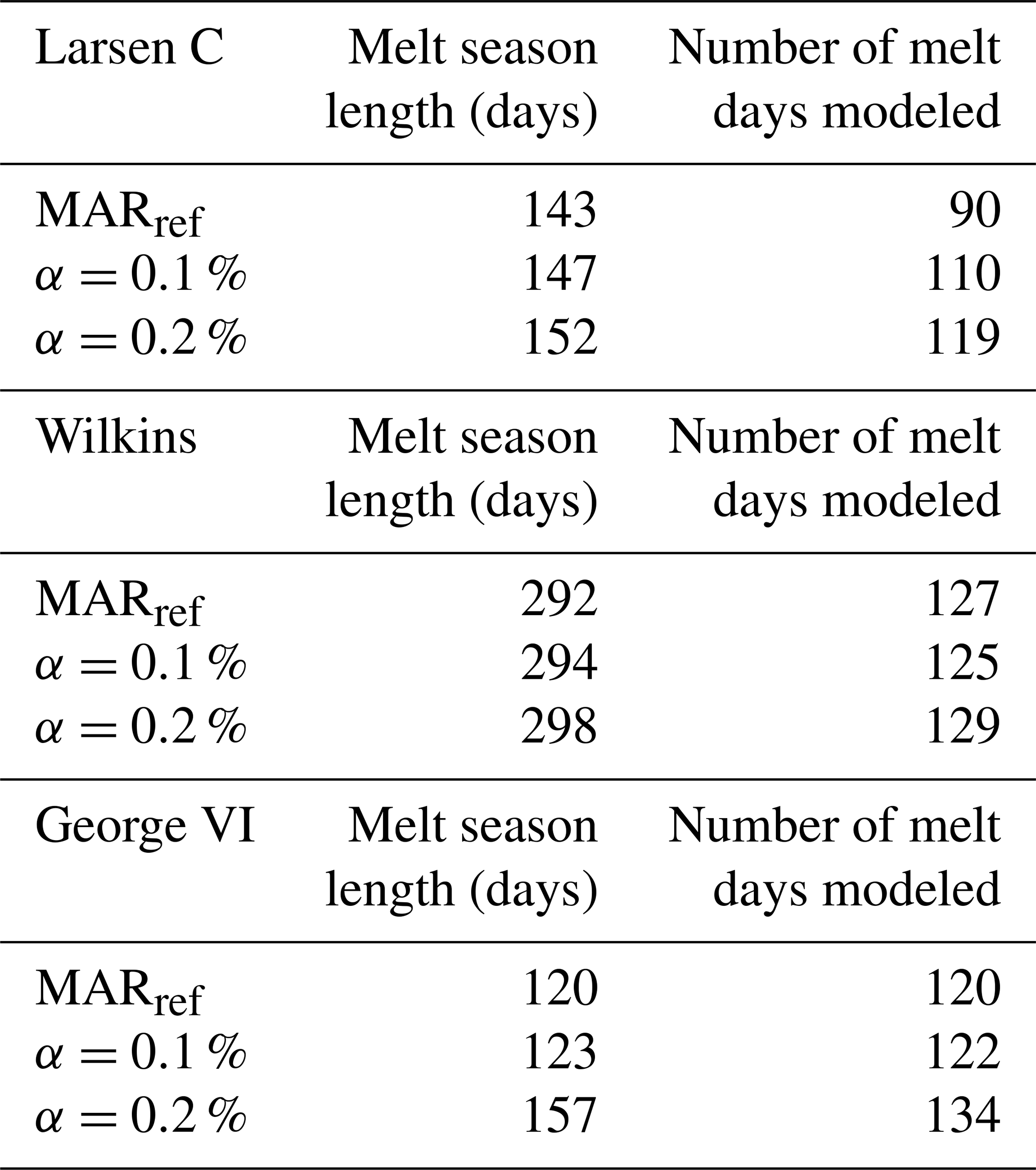
For this study, the number of melt days is defined as the number of days of the melt season where 10 % of the ice shelf experiences melt, while the melt season length corresponds to the number of days between the first melt day after the first of June and the last melt day before the last day of May in the subsequent year. Thus, the melt season length also encompasses possible colder periods where no melting occurs.
Table 7The melt season length (first to last melt day) and number of melt days modeled for MARref and the average for assimilation simulations grouped by α value over the three highlighted ice shelves in Fig. 1 for 2019–2020. A melt day over an ice shelf is a day where more than 10 % of the ice shelf is experiencing melt.
The choice of liquid water content threshold also influences the average number of melt days on the studied ice shelves (Fig. 11). A pixel is considered as melting for the day if the daily averaged mass of liquid water within the first meter of snow is greater than 0.1 % of the snowpack mass. Therefore, using the 0.2 % threshold over 0.1 % will increase the number of melt days.
By computing the mean value of the number of melt days for each ice shelf pixel, it was found that Larsen C is the most sensitive to the threshold chosen, with an increase of 15 melt days compared to MARref. The other two ice shelves exhibit comparatively smaller differences, with Wilkins and George VI experiencing an increase of 8 and 9 melt days, respectively (Fig. 11).
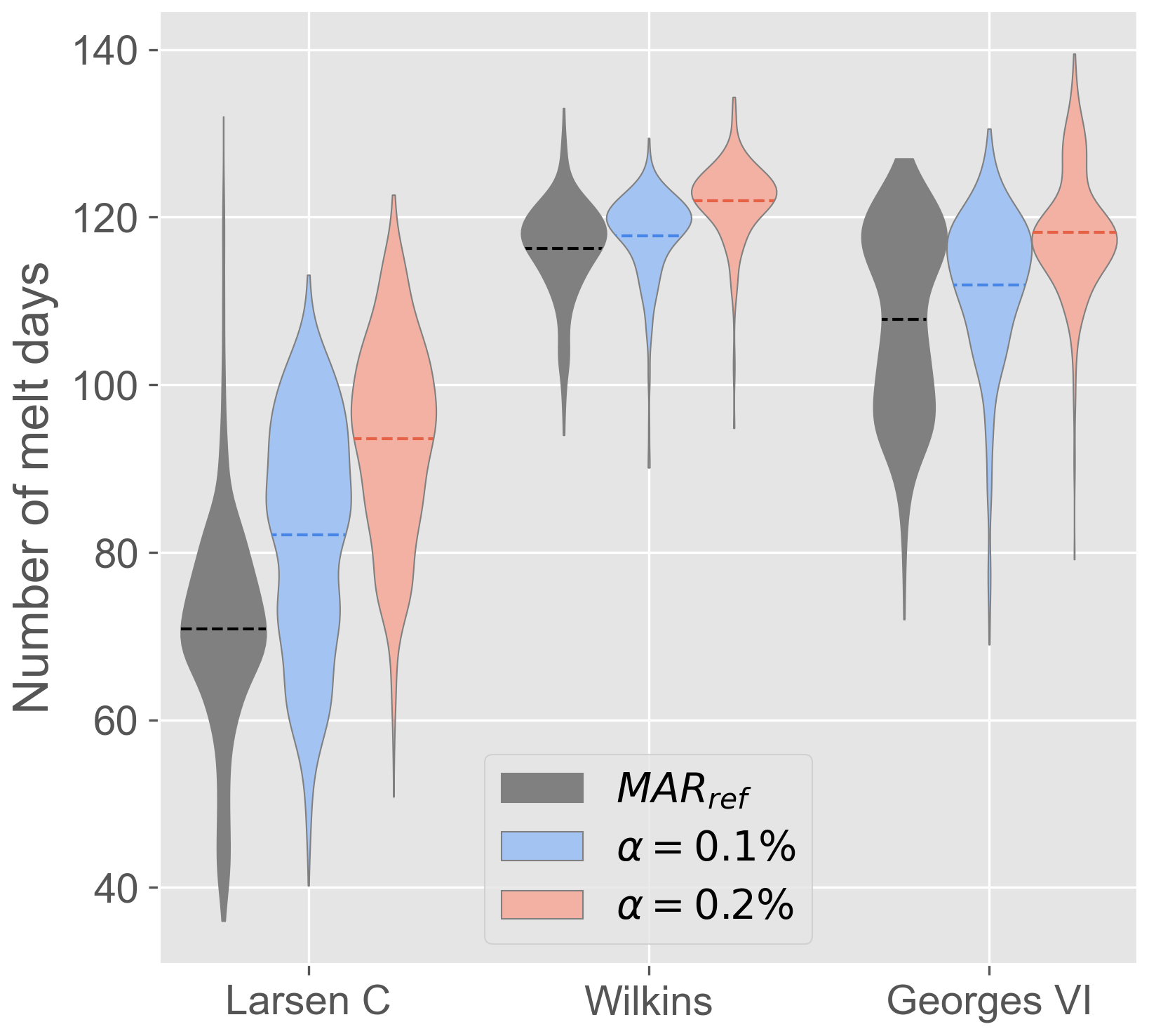
Figure 11Distribution of the number of melt days for the 2019–2020 melt season as modeled by MARref and the assimilations grouped by the specified α threshold values for the three studied ice shelves. Dashed lines represent the mean value of the distribution. On the three ice shelves, assimilations with α=0.2 % produce more melt days than MARref and the other assimilations. Assimilations with α=0.2 % exhibit an increase in the mean number of melt days relative to MARref over the Larsen C ice shelf of 15 d, 8 d on the Wilkins ice shelf and 9 d on the George VI ice shelf.
Examining assimilation simulations individually leads to a similar conclusion. It is important to note that the simulations that were discarded from the computation of are assimilations that had 0.2 % as the value for the threshold. With a densified snowpack, reaching α=0.2 % required more intense melting producing unrealistic surface conditions.
4.1.3 Sensitivity to the RS dataset
In another set of sensitivity experiments, each of the four wet-snow masks (AMSR2 desc., AMSR2 asc., ASCAT, S1) has been assimilated individually into MAR to study its influence. Assimilating multiple datasets tends to smooth the sensor characteristics as they are only processed to be used where they provide consistent information. In this study, several characteristics of the remote sensing data are examined, including the acquisition time, the spatial resolution, and the revisit time, and their impact is discussed below. First, an earlier acquisition time can artificially lower the number of melt days. Because of the daily cycle of the water quantity in the snowpack, images taken earlier in the morning are less likely to observe wet snow (Picard and Fily, 2006). Over the Antarctic Peninsula, the descending orbit of AMSR2 therefore observes less wet snow than the ascending one. Using satellites whose acquisition times are well distributed during the day allows for observation of the daily melt–refreezing cycle and reduces the possibility of excluding melt days.
Second, the spatial resolution influences the results of the assimilation because of pixel heterogeneity. Sensors that have a coarser resolution hide highly heterogeneous surface dynamics, and it is possible that while only a fraction of the region covered by one pixel is experiencing melting or enough water is present in the snowpack, the entire pixel is characterized as wet snow Picard et al. (2022). In steep regions, e.g., near the grounding line, this phenomenon can lead to the detection of wet snow in places where it is unlikely to occur. In this study, the passive microwave sensor AMSR2 has a coarser resolution than MAR and can trigger the assimilation process in locations where it should not be applied.
To study the influence of the spatial resolution, we have performed a simulation assimilating ASCAT data (AsA01S110AMA02AS02 in Table 2) instead of AMSR2 in the descending orbit. The assimilation with ASCAT produces a smaller number of melt days and surface melt production on the Antarctic Peninsula for the studied period (191 Gt yr−1 for AsA01S110AMA02AS02 and 214 Gt yr−1 for Assimref). While the assimilation depth is different between AMSR2 and ASCAT, the major influence comes from the spatial resolution of the sensor (with ASCAT having a higher spatial resolution). The difference can be seen in the wet-snow masks (Fig. 12). AMSR2 detects melt on Alexander Island, between George VI and Wilkins ice shelves, whereas ASCAT with a finer resolution and a different frequency does not. Even if wet snow is observed for one of the AMSR2 masks, the duration of the increased MAR snowpack temperature is too short to produce the water quantities necessary to be detected as melt. This preservation of a cold snowpack persists throughout the day.
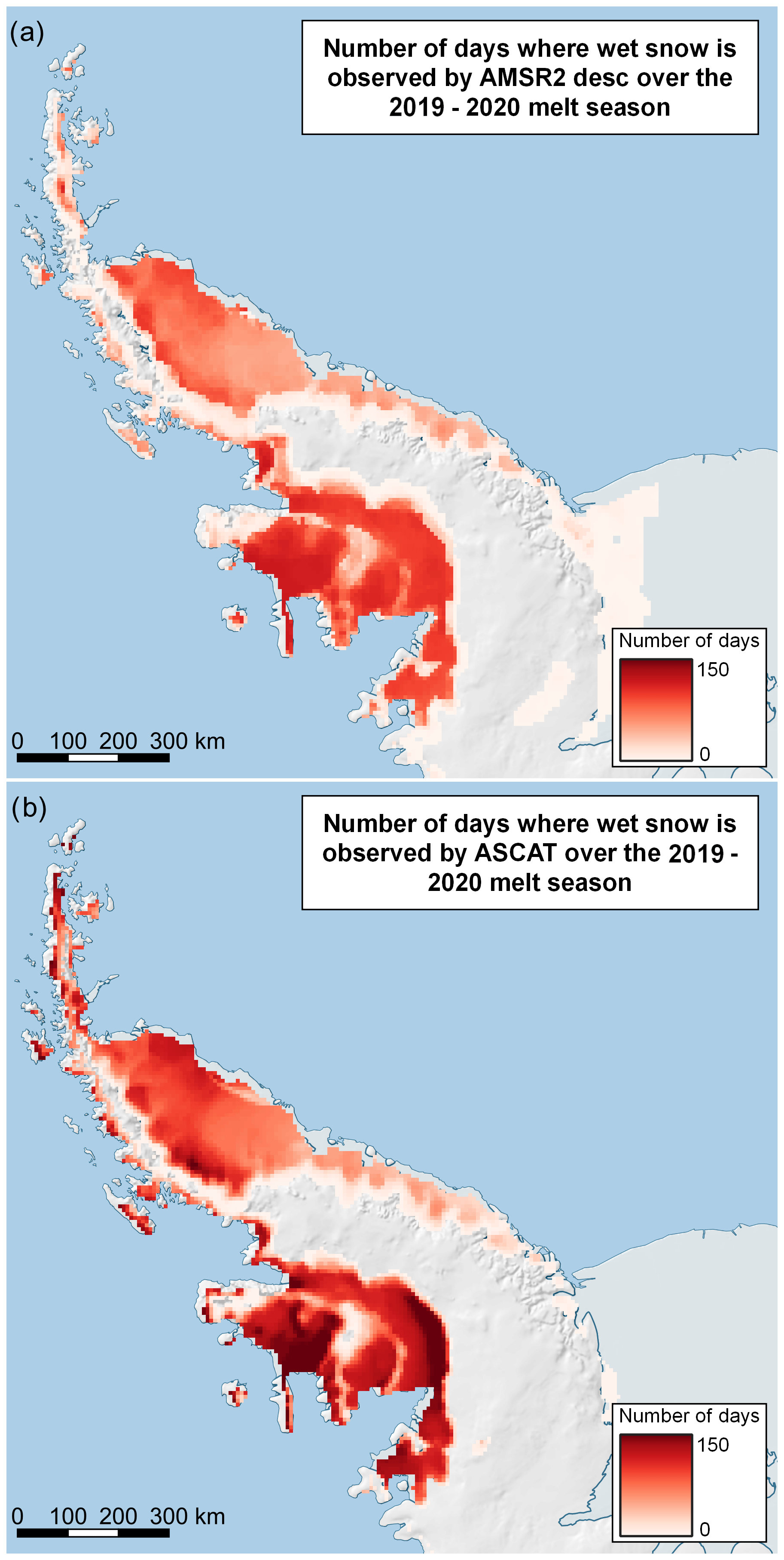
Figure 12(a) Number of days with wet snow observed by AMSR2 ascending on the AP for the 2019–2020 melt season. (b) Number of days with wet snow observed by ASCAT on the Antarctic Peninsula for the 2019–2020 melt season. ASCAT observes more wet snow than AMSR2 over the ice shelves but less melt on average at higher altitudes and in areas of steep terrain.
Finally, the impact of revisit time is highlighted by studying the wet-snow extent resulting from the assimilation of only one sensor at a time (Fig. 13). The assimilated S1 wet-snow mask does not cover the entire AP every day and thus shows a smaller wet-snow extent than the other masks. As a consequence, there are fewer instances in which the model and the mask exhibit discrepancies regarding the snow status, resulting in reduced application of the nudging technique. Ultimately, the S1-only assimilation (AsA01S110 in Table 2) has the closest wet-snow extent to MARref, despite the bias in the raw data. The resilience of the model snowpack is such that relying solely on a non-daily dataset with intermittent nudging allows it to freely evolve with minimal external forcing. Consequently, while the high spatial resolution of Sentinel-1 provides valuable information, this advantage is not sufficient enough to be used as the only dataset assimilated. The S1 dataset needs to be used in conjunction with other datasets to combine high spatial resolution with low revisit time.
The resilience of the snowpack simulation also decreases the feasibility of assimilating only one dataset using the algorithm described in this paper. While the ASCAT-only assimilation (AsA01AS10 in Table 2) tends to be closest to its wet-snow mask during peaks of melt (end of November 2019, beginning of 2020) or strong refreeze (mid-March 2020), the effects of nudging do not persist over long time periods and necessitate changes in the model to match the observed wet-snow mask.
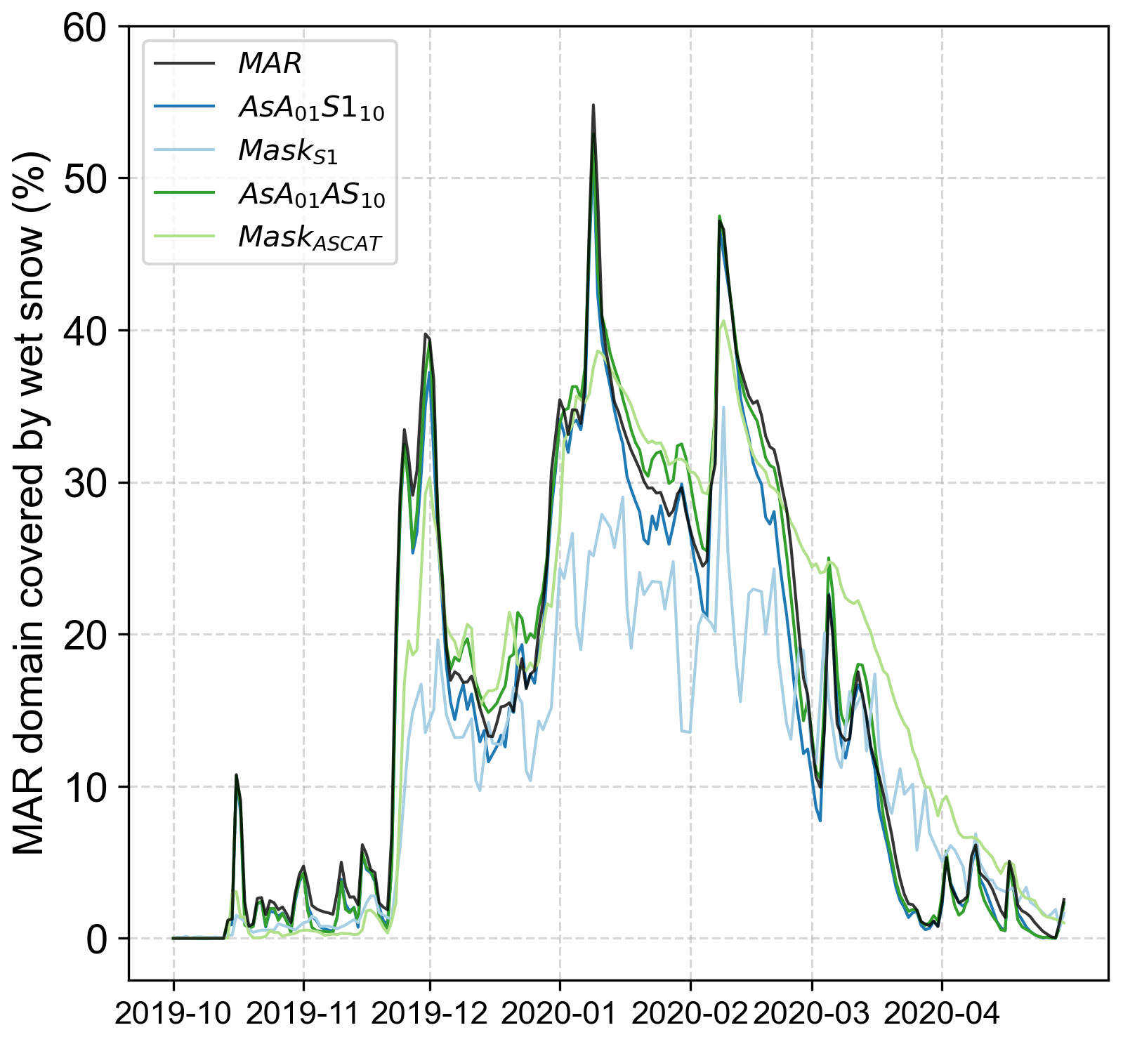
Figure 13Evolution of the wet-snow extent over the entire MAR domain (including grounded ice and ice shelves) during the 2019–2020 melt season as modeled by MARref, the assimilation of S1 alone (AsA01S110), the assimilation of ASCAT alone (AsA01AS10), and the wet-snow masks from S1 and ASCAT. The S1 wet-snow mask has a lower extent as the AP is not covered entirely every day by S1 images.
Assimilating two datasets that entirely cover the study area and a dataset that has a finer spatial resolution compared to MAR serves as a means of mitigating the sensitivity of the model to the chosen datasets. The constraints on the period in which the model snowpack temperature can be changed and the possibility of not assimilating data in case of a discrepancy between the sensors also regulates the dependence of the model on the observations. Future developments in the technique should allow for the possibility of assimilating additional datasets and weighting wet-snow masks according to the relevance of their wet- or dry-snow status.
In this paper, we presented results regarding the assimilation of wet-snow occurrence data estimated by spaceborne microwave sensors into the regional climate model MAR through adjustments in MAR near-surface temperature to best match the satellite data. Sensitivity tests have been performed to evaluate the effect of the data assimilation parameters on the model results.
We identified the assimilation depth (Δz) to be the most influential parameter when applied for shallow-penetration sensors. The influence on the quantity of water produced in the snowpack partially comes from the liquid water content threshold (α) calculation. The uppermost layer of the snowpack is considerably more dense than the underlying layers, owing to the increase in refreezing caused by the exceeding liquid meltwater produced as a result of the assimilation. Heavier and denser layers require more liquid water to be present to reach the required α threshold. In addition, the densification causes firn air content depletion, leaving less space for liquid water. The densified layer saturates faster, and more runoff occurs. A threshold of 0.2 m for the Ku-band sensors causes no extreme refreezing or melt and may be considered a good candidate for assimilation depth thresholds. For the C-band sensors, the three thresholds tested yield similar results to one another, and the implementation of a varying threshold should be considered to take into account the depth at which the wet snow is observed. In contrast to assimilation depth (Δz), the maximum LWC threshold (α) has a smaller impact on the model surface melt production (in Gt). The choice of α=0.2 % over α=0.1 % mostly increases the duration of the melting season, rather than the amount of meltwater produced.
With constant snowfall (480 Gt yr−1) and an increase in surface meltwater production (+95 Gt yr−1 or +66.7 %)), the increase in runoff (+21 Gt yr−1 or +63.8 %)) associated with assimilation translates into a decrease in SMB (−4.5 %)) for the 2019–2020 melt season. Nonetheless, runoff values are relatively small compared to the surface mass balance, explaining the small impact of assimilation on the SMB. The general tendency of SMB remains positive in the study area. Only the ice shelves show negative SMB during periods of intense melting.
The choice of the dataset to be assimilated was also found to influence the results of the model after data assimilation. Each sensor has its particularities, and wet-snow masks may differ between sensors. Several of these characteristics have been pinpointed previously. The most important ones are the signal frequency, the revisit time and the spatial resolution.
The frequency of the sensor impacts estimated meltwater production due to differences in sensitivity to liquid water and the depth to which the signal penetrates. Because it is difficult to provide accurate surface water depth estimates (Fricker et al., 2021) and microwave signals can be intercepted by the water in the snowpack, the vertical limit necessary for the assimilation is not always clear. If there is enough water in the near-surface layers, additional liquid water within deeper layers cannot be observed. In the same way, a thin layer of surface water can be interpreted as the presence of water in the first meter of the snowpack when the underlying layers are dry (Fig. 5). The assimilation depth threshold Δz has been set to different values depending on sensor wavelengths, but remains constant regardless of the snowpack state. Introducing a density-varying LWC threshold could decrease meltwater production in the assimilation simulations. However, we encourage field observations of the evolution of the LWC vertical profile; a required step needed in introducing and validating the assimilation algorithm.
The revisit time of the satellites is influential as the model freely evolves if the forcing is not performed every day. The assimilation of only Sentinel-1 satellites (with a revisit time of 6 d, translating into one image every 2–3 d over the study area) produces results close to those of the model simulation without data assimilation. Multiple datasets need to be assimilated on the same day for the model to consistently change its behavior. The resilience of the model results from the refreezing of the snowpack during nights and in winter months. When taking into account a few melt seasons, at the beginning of the melt season the model snowpack is more or less similar to its state in the previous year.
Assimilating multiple datasets into MAR also brings challenges and considerations alongside the advantages. If some missing information is fulfilled by another dataset, it adds another layer of complexity to the algorithm or additional uncertainties linked to the assimilation method used and its thresholds. Datasets may not carry the same information and may not be compatible for all the time steps. Here, none of the datasets is considered to have better wet-snow detection than the other. A possible enhancement of the technique would be to add weight to the masks in case of contradictions between them. The weight could be constructed using the confidence level of the wet-snow detection technique employed, the satellite spatial resolution, the topographic gradient from higher-resolution satellite pixels interpolated to the MAR grid or the sensor sensitivity to liquid water.
The results highlight the importance and impact of utilizing data assimilation. While the assimilation does not induce a complete change in the behavior of the model as surface melt remains marginal to snowfall, the snowpack properties tend to deviate from the model simulation performed without assimilation, impacting the ability of the snowpack to retain meltwater in the future. Here, satellite data have only been assimilated for two melt seasons over a small area. The study can be expanded in the future to cover a longer period, a larger spatial extent, or the Greenland Ice Sheet, where surface melt is the main driver of SMB variability (Slater et al., 2021). Further attention should be given to ice shelves as they are the most sensitive region of Antarctica and important to the Antarctic ice sheet stability (Favier and Pattyn, 2015; Paolo et al., 2015; Sun et al., 2020).
Finally, The results obtained in this paper pinpoint the uncertainties in the regional climate model over the Antarctic Peninsula, where, without significant increases in simulated melt area, the surface melt production significantly increased. The assimilation of remotely sensed data into RCMs is a promising way of reducing the biases and errors inherent to climate models, given that there are currently no direct large-scale measurement of meltwater content within the Antarctic snowpack. This is also an easy way to provide robust uncertainties in model outputs for present climate. Using multiple RS datasets with spatial resolutions higher than the model resolution would also allow for improved model corrections through better assessment of the snowpack water content.
The MAR code used in this study is tagged as v3.12 on https://gitlab.com/Mar-Group/MARv3 (MAR Team, 2022). Instructions to download the MAR code are provided at https://www.mar.cnrs.fr (last access: 10 November 2022) (MAR model, 2022). The MAR outputs used in this study are available upon request by email (tdethinne@uliege.be). Python code and the necessary files to perform the assimilation with MAR are available on Zenodo (https://doi.org/10.5281/zenodo.8391577 (Dethinne, 2023).
The supplement related to this article is available online at: https://doi.org/10.5194/tc-17-4267-2023-supplement.
TD, QG and XF conceived the study. TD performed the simulations based on a domain created by CK. TD led the writing of the manuscript. TD, QG, GP, XF, CK, PA and AO discussed the results. TD and GP processed the RS data. CK assisted with AWS data comparison. All co-authors revised and contributed to the editing of the manuscript.
At least one of the (co-)authors is a member of the editorial board of The Cryosphere. The peer-review process was guided by an independent editor, and the authors also have no other competing interests to declare.
Publisher's note: Copernicus Publications remains neutral with regard to jurisdictional claims in published maps and institutional affiliations.
We thank Charles Zender and the two anonymous reviewers for their constructive comments that greatly improved the study.
ERA5 reanalysis data (Hersbach et al., 2020) are provided by the European Centre for Medium-Range Weather Forecasts, available at https://www.ecmwf.int/en/forecasts/datasets/reanalysis-datasets/era5 (last access: 24 October 2022).
We acknowledge the contribution of the Consortium des Équipements de Calcul Intensif (CÉCI), funded by the Fonds de la Recherche Scientifique de Belgique (F.R.S. – FNRS) under grant no. 2.5020.11 and the Tier-1 supercomputer (Nic5) of the Fédération Wallonie Bruxelles infrastructure funded by the Walloon Region under grant agreement no. 1117545.
Background maps have been provided by the Norwegian Polar Institute through the Quantarctica3 project (Matsuoka et al., 2021).
This project is partially carried out within the framework of the Digital Twin Antarctica Project of the European Space Agency (ESA, contract no. 4000128611/19/I- DT).
This research has been supported by the Spheres Research Unit from Liège University.
This paper was edited by Tobias Sauter and reviewed by Charles Zender and two anonymous referees.
Adusumilli, S., Fricker, H. A., Medley, B., Padman, L., and Siegfried, M. R.: Interannual variations in meltwater input to the Southern Ocean from Antarctic ice shelves, Nat. Geosci., 13, 616–620, https://doi.org/10.1038/s41561-020-0616-z, 2020. a
Amante, C. and Eakins, B. W.: ETOPO1 arc-minute global relief model: procedures, data sources and analysis, NOAA technical memorandum NESDIS NGDC-24, https://repository.library.noaa.gov/view/noaa/1163 (last access: 20 October 2022), 2009. a
Ashcraft, I. S. and Long, D. G.: Comparison of methods for melt detection over Greenland using active and passive microwave measurements, Int. J. Remote Sens., 27, 2469–2488, https://doi.org/10.1080/01431160500534465, 2006. a
Banwell, A. F., Datta, R. T., Dell, R. L., Moussavi, M., Brucker, L., Picard, G., Shuman, C. A., and Stevens, L. A.: The 32-year record-high surface melt in 2019/2020 on the northern George VI Ice Shelf, Antarctic Peninsula, The Cryosphere, 15, 909–925, https://doi.org/10.5194/tc-15-909-2021, 2021. a
Barrand, N. E., Vaughan, D. G., Steiner, N., Tedesco, M., Kuipers Munneke, P., van den Broeke, M. R., and Hosking, J. S.: Trends in Antarctic Peninsula surface melting conditions from observations and regional climate modeling, J. Geophys. Res.-Earth Surf., 118, 315–330, https://doi.org/10.1029/2012JF002559, 2013. a
Bell, R. E., Banwell, A. F., Trusel, L. D., and Kingslake, J.: Antarctic surface hydrology and impacts on ice-sheet mass balance, Nat. Clim. Change, 8, 1044–1052, https://doi.org/10.1038/s41558-018-0326-3, 2018. a, b
Brun, E., David, P., Sudul, M., and Brunot, G.: A numerical model to simulate snow-cover stratigraphy for operational avalanche forecasting, J. Glaciol., 38, 13–22, https://doi.org/10.3189/s0022143000009552, 1992. a
Church, J., Clark, P., Cazenave, A., Gregory, J., Jevrejeva, S., Levermann, A., Merrifield, M., Milne, G., Nerem, R., Nunn, P., Payne, A., Pfeffer, W., Stammer, D., and Unnikrishnan, A.: Sea Level Change, in: Climate Change 2013: The Physical Science Basis. Contribution of Working Group I to the Fifth Assessment Report of the Intergovernmental Panel on Climate Change, edited by: Stocker, T., Qin, D., Plattner, G.-K., Tignor, M., Allen, S., Boschung, J., Nauels, A., Xia, Y., Bex, V., and Midgley, P., Cambridge University Press, Cambridge, United Kingdom and New York, NY, USA, https://www.ipcc.ch/site/assets/uploads/2018/02/WG1AR5_Chapter13_FINAL.pdf (last access: 6 October 2023), 2013. a
Chuter, S. J., Zammit-Mangion, A., Rougier, J., Dawson, G., and Bamber, J. L.: Mass evolution of the Antarctic Peninsula over the last 2 decades from a joint Bayesian inversion, The Cryosphere, 16, 1349–1367, https://doi.org/10.5194/tc-16-1349-2022, 2022. a, b
Coléou, C. and Lesaffre, B.: Irreducible water saturation in snow: Experimental results in a cold laboratory, Ann. Glaciol., 26, 64–68, https://doi.org/10.1017/S0260305500014579, 1998. a
Colosio, P., Tedesco, M., Ranzi, R., and Fettweis, X.: Surface melting over the Greenland ice sheet derived from enhanced resolution passive microwave brightness temperatures (1979–2019), The Cryosphere, 15, 2623–2646, https://doi.org/10.5194/tc-15-2623-2021, 2021. a, b
Datta, R. T., Tedesco, M., Agosta, C., Fettweis, X., Kuipers Munneke, P., and van den Broeke, M. R.: Melting over the northeast Antarctic Peninsula (1999–2009): evaluation of a high-resolution regional climate model, The Cryosphere, 12, 2901–2922, https://doi.org/10.5194/tc-12-2901-2018, 2018. a, b
Datta, R. T., Tedesco, M., Fettweis, X., Agosta, C., Lhermitte, S., Lenaerts, J. T. M., and Wever, N.: The Effect of Foehn-Induced Surface Melt on Firn Evolution Over the Northeast Antarctic Peninsula, Geophys. Res. Lett., 46, 3822–3831, https://doi.org/10.1029/2018GL080845, 2019. a
Delhasse, A., Kittel, C., Amory, C., Hofer, S., van As, D., S. Fausto, R., and Fettweis, X.: Brief communication: Evaluation of the near-surface climate in ERA5 over the Greenland Ice Sheet, The Cryosphere, 14, 957–965, https://doi.org/10.5194/tc-14-957-2020, 2020. a, b
Dethinne, T.: MAR RS assimilation, Zenodo [code], https://doi.org/10.5281/zenodo.8391577, 2023. a
Donat-Magnin, M., Jourdain, N. C., Kittel, C., Agosta, C., Amory, C., Gallée, H., Krinner, G., and Chekki, M.: Future surface mass balance and surface melt in the Amundsen sector of the West Antarctic Ice Sheet, The Cryosphere, 15, 571–593, https://doi.org/10.5194/tc-15-571-2021, 2021. a
Elachi, C. and van Zyl, J.: Nature and Properties of Electromagnetic Waves, in: Introduction to the Physics and Techniques of Remote Sensing, Chap. 2, 23–50, John Wiley and Sons, Ltd, https://doi.org/10.1002/0471783390.ch2, 2006. a, b
ESA: The Sentinel-1 Toolbox, https://sentinel.esa.int/web/sentinel/toolboxes/sentinel-1 (last access: 19 October 2022), 2022. a
ESA: Sentinel-1, https://sentinel.esa.int/web/sentinel/missions/sentinel-1 (last access: 24 May 2023), 2023. a
EUMETSAT: ASCAT Level 1 Sigma0 Full Resolution – Metop – Global, https://navigator.eumetsat.int/product/EO:EUM:DAT:METOP:ASCSZF1B (last access: 24 May 2023), 2023. a, b
Evensen, G.: Data assimilation: The ensemble kalman filter, Springer Berlin, Heidelberg, https://doi.org/10.1007/978-3-642-03711-5, 2009. a
Fahnestock, M. A., Abdalati, W., and Shuman, C. A.: Long melt seasons on ice shelves of the Antarctic Peninsula: an analysis using satellite-based microwave emission measurements, Ann. Glaciol., 34, 127–133, https://doi.org/10.3189/172756402781817798, 2002. a
Favier, L. and Pattyn, F.: Antarctic ice rise formation, evolution, and stability, Geophys. Res. Lett., 42, 4456–4463, https://doi.org/10.1002/2015GL064195, 2015. a, b
Fettweis, X., Tedesco, M., van den Broeke, M., and Ettema, J.: Melting trends over the Greenland ice sheet (1958–2009) from spaceborne microwave data and regional climate models, The Cryosphere, 5, 359–375, https://doi.org/10.5194/tc-5-359-2011, 2011. a
Fettweis, X., Hofer, S., Séférian, R., Amory, C., Delhasse, A., Doutreloup, S., Kittel, C., Lang, C., Van Bever, J., Veillon, F., and Irvine, P.: Brief communication: Reduction in the future Greenland ice sheet surface melt with the help of solar geoengineering, The Cryosphere, 15, 3013–3019, https://doi.org/10.5194/tc-15-3013-2021, 2021. a
Fretwell, P., Pritchard, H. D., Vaughan, D. G., Bamber, J. L., Barrand, N. E., Bell, R., Bianchi, C., Bingham, R. G., Blankenship, D. D., Casassa, G., Catania, G., Callens, D., Conway, H., Cook, A. J., Corr, H. F. J., Damaske, D., Damm, V., Ferraccioli, F., Forsberg, R., Fujita, S., Gim, Y., Gogineni, P., Griggs, J. A., Hindmarsh, R. C. A., Holmlund, P., Holt, J. W., Jacobel, R. W., Jenkins, A., Jokat, W., Jordan, T., King, E. C., Kohler, J., Krabill, W., Riger-Kusk, M., Langley, K. A., Leitchenkov, G., Leuschen, C., Luyendyk, B. P., Matsuoka, K., Mouginot, J., Nitsche, F. O., Nogi, Y., Nost, O. A., Popov, S. V., Rignot, E., Rippin, D. M., Rivera, A., Roberts, J., Ross, N., Siegert, M. J., Smith, A. M., Steinhage, D., Studinger, M., Sun, B., Tinto, B. K., Welch, B. C., Wilson, D., Young, D. A., Xiangbin, C., and Zirizzotti, A.: Bedmap2: improved ice bed, surface and thickness datasets for Antarctica, The Cryosphere, 7, 375–393, https://doi.org/10.5194/tc-7-375-2013, 2013. a
Fricker, H. A., Arndt, P., Brunt, K. M., Datta, R. T., Fair, Z., Jasinski, M. F., Kingslake, J., Magruder, L. A., Moussavi, M., Pope, A., Spergel, J. J., Stoll, J. D., and Wouters, B.: ICESat-2 Meltwater Depth Estimates: Application to Surface Melt on Amery Ice Shelf, East Antarctica, Geophys. Res. Lett., 48, e2020GL090550, https://doi.org/10.1029/2020GL090550, 2021. a, b
Gallée, H. and Schayes, G.: Development of a Three-Dimensional Meso-γ Primitive Equation Model: Katabatic Winds Simulation in the Area of Terra Nova Bay, Antarctica, Mon. Weather Rev., 122, 671–685, https://doi.org/10.1175/1520-0493(1994)122<0671:DOATDM>2.0.CO;2, 1994. a
GEE: Sentinel-1 Algorithms, https://developers.google.com/earth-engine/guides/sentinel1 (last access: 19 October 2022), 2022. a
Gilbert, E. and Kittel, C.: Surface Melt and Runoff on Antarctic Ice Shelves at 1.5 °C, 2 °C, and 4 °C of Future Warming, Geophys. Res. Lett., 48, 9, https://doi.org/10.1029/2020GL091733, 2021. a, b
Glaude, Q., Amory, C., Berger, S., Derauw, D., Pattyn, F., Barbier, C., and Orban, A.: Empirical Removal of Tides and Inverse Barometer Effect on DInSAR From Double DInSAR and a Regional Climate Model, IEEE J. Sel. Top. Appl. Earth Obs., 13, 4085–4094, https://doi.org/10.1109/JSTARS.2020.3008497, 2020. a
Gorelick, N., Hancher, M., Dixon, M., Ilyushchenko, S., Thau, D., and Moore, R.: Google Earth Engine: Planetary-scale geospatial analysis for everyone, Remote Sens. Environ., 202, 18–27, https://doi.org/10.1016/j.rse.2017.06.031, 2017. a
Hersbach, H., Bell, B., Berrisford, P., Hirahara, S., Horányi, A., Muñoz-Sabater, J., Nicolas, J., Peubey, C., Radu, R., Schepers, D., Simmons, A., Soci, C., Abdalla, S., Abellan, X., Balsamo, G., Bechtold, P., Biavati, G., Bidlot, J., Bonavita, M., De Chiara, G., Dahlgren, P., Dee, D., Diamantakis, M., Dragani, R., Flemming, J., Forbes, R., Fuentes, M., Geer, A., Haimberger, L., Healy, S., Hogan, R. J., Hólm, E., Janisková, M., Keeley, S., Laloyaux, P., Lopez, P., Lupu, C., Radnoti, G., de Rosnay, P., Rozum, I., Vamborg, F., Villaume, S., and Thépaut, J.-N.: The ERA5 global reanalysis, Q. J. Roy. Meteor. Soc., 146, 1999–2049, https://doi.org/10.1002/qj.3803, 2020. a, b, c
Husman, S. D. R., Zhongyang, H., Wouters, B., Munneke, P. K., Veldhuijsen, S., and Lhermitte, S.: Remote Sensing of Surface Melt on Antarctica: Opportunities and Challenges, J. Sel. Top. Appl. Earth Obs., 16, 2462–2480, https://doi.org/10.1109/JSTARS.2022.3216953, 2022. a
Jakobs, C. L., Reijmer, C. H., Smeets, C. J., Trusel, L. D., Berg, W. J. V. D., Broeke, M. R. V. D., and Wessem, J. M. V.: A benchmark dataset of in situ Antarctic surface melt rates and energy balance, J. Glaciol., 66, 291–302, https://doi.org/10.1017/jog.2020.6, dataset, 2020. a, b
JAXA: Globe portal system, https://gportal.jaxa.jp/gpr/ (last access: 10 January 2022), 2021. a, b
Johnson, A., Fahnestock, M., and Hock, R.: Evaluation of passive microwave melt detection methods on Antarctic Peninsula ice shelves using time series of Sentinel-1 SAR, Remote Sens. Environ., 250, 112044, https://doi.org/10.1016/j.rse.2020.112044, 2020. a, b, c, d, e, f, g
Johnson, A., Hock, R., and Fahnestock, M.: Spatial variability and regional trends of Antarctic ice shelf surface melt duration over 1979–2020 derived from passive microwave data, J. Glaciol., 68, 533–546, https://doi.org/10.1017/jog.2021.112, 2022. a
Kittel, C.: Present and future sensitivity of the Antarctic surface mass balance to oceanic and atmospheric forcings: insights with the regional climate model MAR, PhD thesis, ULiège – Université de Liège, https://hdl.handle.net/2268/258491 (last access: 28 September 2023), 2021. a
Kittel, C., Amory, C., Agosta, C., Jourdain, N. C., Hofer, S., Delhasse, A., Doutreloup, S., Huot, P.-V., Lang, C., Fichefet, T., and Fettweis, X.: Diverging future surface mass balance between the Antarctic ice shelves and grounded ice sheet, The Cryosphere, 15, 1215–1236, https://doi.org/10.5194/tc-15-1215-2021, 2021. a, b
Kittel, C., Fettweis, X., Picard, G., and Gourmelen, N.: Assimilation of satellite-derived melt extent increases melt simulated by MAR over the Amundsen sector (West Antarctica), Bulletin de la Société Géographique de Liège, 78, 87–99, https://doi.org/10.25518/0770-7576.6616, 2022. a, b, c
Koskinen, J., Pulliainen, J., and Hallikainen, M.: The use of ERS-1 SAR data in snow melt monitoring, IEEE T. Geosci. Remote, 35, 601–610, https://doi.org/10.1109/36.581975, 1997. a
Kuipers Munneke, P., Luckman, A. J., Bevan, S. L., Smeets, C. J. P. P., Gilbert, E., van den Broeke, M. R., Wang, W., Zender, C., Hubbard, B., Ashmore, D., Orr, A., King, J. C., and Kulessa, B.: Intense Winter Surface Melt on an Antarctic Ice Shelf, Geophys. Res. Lett., 45, 7615–7623, https://doi.org/10.1029/2018GL077899, 2018. a
Lai, C.-Y., Kingslake, J., Wearing, M. G., Chen, P.-H. C., Gentine, P., Li, H., Spergel, J. J., and van Wessem, J. M.: Vulnerability of Antarctica’s ice shelves to meltwater-driven fracture, Nature, 584, 574–578, https://doi.org/10.1038/s41586-020-2627-8, 2020. a
Lambin, C., Fettweis, X., Kittel, C., Fonder, M., and Ernst, D.: Assessment of future wind speed and wind power changes over South Greenland using the Modèle Atmosphérique Régional regional climate model, Int. J. Climatol., 43, 558–574, https://doi.org/10.1002/joc.7795, 2022. a
Liang, D., Guo, H., Zhang, L., Cheng, Y., Zhu, Q., and Liu, X.: Time-series snowmelt detection over the Antarctic using Sentinel-1 SAR images on Google Earth Engine, Remote Sens. Environ., 256, 112318, https://doi.org/10.1016/j.rse.2021.112318, 2021. a, b
Lindsley, R. D. and Long, D. G.: Enhanced-Resolution Reconstruction of ASCAT Backscatter Measurements, IEEE T. Geosci. Remote, 54, 2589–2601, https://doi.org/10.1109/TGRS.2015.2503762, 2016. a
MAR model: MAR, http://www.mar.cnrs.fr (last access: 10 November 2022), 2022. a
MAR Team: MARv3.12, MAR Team [code], https://gitlab.com/Mar-Group/ (last access: 16 November 2022), 2022. a
Matsuoka, K., Skoglund, A., Roth, G., de Pomereu, J., Griffiths, H., Headland, R., Herried, B., Katsumata, K., Le Brocq, A., Licht, K., Morgan, F., Neff, P. D., Ritz, C., Scheinert, M., Tamura, T., Van de Putte, A., van den Broeke, M., von Deschwanden, A., Deschamps-Berger, C., Van Liefferinge, B., Tronstad, S., and Melvær, Y.: Quantarctica, an integrated mapping environment for Antarctica, the Southern Ocean, and sub-Antarctic islands, Environ. Model. Softw., 140, 105015, https://doi.org/10.1016/j.envsoft.2021.105015, 2021. a
Morcrette, J.-J.: Assessment of the ECMWF Model Cloudiness and Surface Radiation Fields at the ARM SGP Site, Mon. Weather Rev., 130, 257–277, https://doi.org/10.1175/1520-0493(2002)130<0257:AOTEMC>2.0.CO;2, 2002. a
Moreira, A., Prats-Iraola, P., Younis, M., Krieger, G., Hajnsek, I., and Papathanassiou, K. P.: A tutorial on synthetic aperture radar, IEEE Geosci. Remote Sens. Mag., 1, 6–43, https://doi.org/10.1109/MGRS.2013.2248301, 2013. a
Mottram, R., Hansen, N., Kittel, C., van Wessem, J. M., Agosta, C., Amory, C., Boberg, F., van de Berg, W. J., Fettweis, X., Gossart, A., van Lipzig, N. P. M., van Meijgaard, E., Orr, A., Phillips, T., Webster, S., Simonsen, S. B., and Souverijns, N.: What is the surface mass balance of Antarctica? An intercomparison of regional climate model estimates, The Cryosphere, 15, 3751–3784, https://doi.org/10.5194/tc-15-3751-2021, 2021. a
Mullissa, A., Vollrath, A., Odongo-Braun, C., Slagter, B., Balling, J., Gou, Y., Gorelick, N., and Reiche, J.: Sentinel-1 SAR Backscatter Analysis Ready Data Preparation in Google Earth Engine, Remote Sens., 13, 1954, https://doi.org/10.3390/rs13101954, 2021. a
Mätzler, C.: Applications of the interaction of microwaves with the natural snow cover, Remote Sens. Rev., 2, 259–387, https://doi.org/10.1080/02757258709532086, 1987. a
Nagler, T. and Rott, H.: Retrieval of wet snow by means of multitemporal SAR data, IEEE T. Geosci. Remote, 38, 754–765, https://doi.org/10.1109/36.842004, 2000. a, b
Nagler, T., Rott, H., Ripper, E., Bippus, G., and Hetzenecker, M.: Advancements for Snowmelt Monitoring by Means of Sentinel-1 SAR, Remote Sens., 8, 348, https://doi.org/10.3390/rs8040348, 2016. a
Navari, M., Margulis, S. A., Tedesco, M., Fettweis, X., and Alexander, P. M.: Improving Greenland Surface Mass Balance Estimates Through the Assimilation of MODIS Albedo: A Case Study Along the K-Transect, Geophys. Res. Lett., 45, 6549–6556, https://doi.org/10.1029/2018GL078448, 2018. a
Noël, B., van de Berg, W. J., Lhermitte, S., Wouters, B., Machguth, H., Howat, I., Citterio, M., Moholdt, G., Lenaerts, J. T. M., and van den Broeke, M. R.: A tipping point in refreezing accelerates mass loss of Greenland’s glaciers and ice caps, Nat. Commun., 8, 14730, https://doi.org/10.1038/ncomms14730, 2017. a
Paolo, F. S., Fricker, H. A., and Padman, L.: Volume loss from Antarctic ice shelves is accelerating, Science, 348, 327–331, https://doi.org/10.1126/science.aaa0940, 2015. a, b
Parkinson, C.: Satellite Passive Microwave Measurements of Sea Ice, in: Encyclopedia of Ocean Sciences, edited by: Steele, J. H., Academic Press, Oxford, 2531–2539, https://doi.org/10.1006/rwos.2001.0336, 2001. a
Picard, G. and Fily, M.: Surface melting observations in Antarctica by microwave radiometers: Correcting 26-year time series from changes in acquisition hours, Remote Sens. Environ., 104, 325–336, https://doi.org/10.1016/j.rse.2006.05.010, 2006. a, b
Picard, G., Leduc-Leballeur, M., Banwell, A. F., Brucker, L., and Macelloni, G.: The sensitivity of satellite microwave observations to liquid water in the Antarctic snowpack, The Cryosphere, 16, 5061–5083, https://doi.org/10.5194/tc-16-5061-2022, 2022. a, b, c, d, e, f, g, h
Ridder, K. D. and Gallée, H.: Land Surface-Induced Regional Climate Change in Southern Israel, J. Appl. Meteorol., 37, 1470–1485, https://doi.org/10.1175/1520-0450(1998)037<1470:LSIRCC>2.0.CO;2, 1998. a
Rignot, E., Mouginot, J., Scheuchl, B., van den Broeke, M., van Wessem, M. J., and Morlighem, M.: Four decades of Antarctic Ice Sheet mass balance from 1979–2013;2017, P. Natl. Acad. Sci. USA, 116, 1095–1103, https://doi.org/10.1073/pnas.1812883116, 2019. a, b
Scambos, T., Hulbe, C., and Fahnestock, M.: Climate-Induced Ice Shelf Disintegration in the Antarctic Peninsula, in: Antarctic Peninsula Climate Variability: Historical and Paleoenvironmental Perspectives, American Geophysical Union, 79–92, https://doi.org/10.1029/AR079p0079, 2003. a
Slater, T., Shepherd, A., McMillan, M., Leeson, A., Gilbert, L., Muir, A., Munneke, P. K., Noël, B., Fettweis, X., van den Broeke, M., and Briggs, K.: Increased variability in Greenland Ice Sheet runoff from satellite observations, Nat. Commun., 12, 6069, https://doi.org/10.1038/s41467-021-26229-4, 2021. a
Sun, S., Pattyn, F., Simon, E. G., Albrecht, T., Cornford, S., Calov, R., Dumas, C., Gillet-Chaulet, F., Goelzer, H., Golledge, N. R., Greve, R., Hoffman, M. J., Humbert, A., Kazmierczak, E., Kleiner, T., Leguy, G. R., Lipscomb, W. H., Martin, D., Morlighem, M., Nowicki, S., Pollard, D., Price, S., Quiquet, A., Seroussi, H., Schlemm, T., Sutter, J., van de Wal, R. S. W., Winkelmann, R., and Zhang, T.: Antarctic ice sheet response to sudden and sustained ice-shelf collapse (ABUMIP), J. Glaciol., 66, 891–904, https://doi.org/10.1017/jog.2020.67, 2020. a
Tedesco, M., Abdalati, W., and Zwally, H. J.: Persistent surface snowmelt over Antarctica (1987–2006) from 19.35 GHz brightness temperatures, Geophys. Res. Lett., 34, 1–6, https://doi.org/10.1029/2007GL031199, 2007. a
The IMBIE Team: Mass balance of the Antarctic Ice Sheet from 1992 to 2017, Nature, 558, 219–222, https://doi.org/10.1038/s41586-018-0179-y, 2018. a
Trusel, L. D., Frey, K. E., Das, S. B., Munneke, P. K., and van den Broeke, M. R.: Satellite-based estimates of Antarctic surface meltwater fluxes, Geophys. Res. Lett., 40, 6148–6153, https://doi.org/10.1002/2013GL058138, 2013. a
Trusel, L. D., Frey, K. E., Das, S. B., Karnauskas, K. B., Munneke, P. K., Meijgaard, E. V., and Broeke, M. R. V. D.: Divergent trajectories of Antarctic surface melt under two twenty-first-century climate scenarios, Nat. Geosci., 8, 927–932, https://doi.org/10.1038/ngeo2563, 2015. a
Van Tricht, K., Lhermitte, S., Lenaerts, J. T. M., Gorodetskaya, I. V., L'Ecuyer, T. S., Noël, B., van den Broeke, M. R., Turner, D. D., and van Lipzig, N. P. M.: Clouds enhance Greenland ice sheet meltwater runoff, Nat. Commun., 7, 10266, https://doi.org/10.1038/ncomms10266, 2016. a
Wille, J. D., Favier, V., Jourdain, N. C., Kittel, C., Turton, J. V., Agosta, C., Gorodetskaya, I. V., Picard, G., Codron, F., Santos, C. L.-D., Amory, C., Fettweis, X., Blanchet, J., Jomelli, V., and Berchet, A.: Intense atmospheric rivers can weaken ice shelf stability at the Antarctic Peninsula, Commun. Earth Environ., 3, 90, https://doi.org/10.1038/s43247-022-00422-9, 2022. a
Zwally, H. J. and Fiegles, S.: Extent and duration of Antarctic surface melting, J. Glaciol., 40, 463–475, https://doi.org/10.3189/s0022143000012338, 1994. a, b, c
Modèle Atmosphérique Régional(MAR) to the assimilation of wet-snow occurrence estimated by remote sensing datasets. The assimilation is performed by nudging the MAR snowpack temperature. The data assimilation is performed over the Antarctic Peninsula for the 2019–2021 period. The results show an increase in the melt production (+66.7 %) and a decrease in surface mass balance (−4.5 %) of the model for the 2019–2020 melt season.
Modèle Atmosphérique Régional(MAR)...