the Creative Commons Attribution 4.0 License.
the Creative Commons Attribution 4.0 License.
 | 25 Sep 2023
Brief communication: Identification of tundra topsoil frozen/thawed state from SMAP and GCOM-W1 radiometer measurements using the spectral gradient method
Konstantin Muzalevskiy
Zdenek Ruzicka
Alexandre Roy
Michael Loranty
Alexander Vasiliev
From 2015 to 2020, using the spectral gradient radiometric method, the possibility of the frozen/thawed (FT) state identification of tundra soil was investigated based on Soil Moisture Active Passive (SMAP) and Global Change Observation Mission – Water Satellite 1 (GCOM-W1) satellite observations of 10 test sites located in the Arctic regions of Canada, Finland, Russia, and the USA. It is shown that the spectral gradients of brightness temperature and reflectivity (measured in the frequency range from 1.4 to 36.5 GHz with horizontal polarization, a determination coefficient from 0.775 to 0.834, a root-mean-square error from 6.6 to 10.7 d and a bias from −3.4 to +6.5 d) make it possible to identify the FT state of the tundra topsoil. The spectral gradient method has a higher accuracy with respect to the identification of the FT state of tundra soils than single-frequency methods based on the calculation of polarization index.
- Article
(2042 KB) - Full-text XML
- BibTeX
- EndNote


Microwave radiometry is a promising all-weather method for the remote sensing of seasonal soil thawing and freezing cycles in the Arctic region. The microwave emission changes significantly at the phase transitions of water in wet soil, thereby making it possible to identify the frozen/thawed (FT) state of the soil. Recently, both single- and multifrequency radiometric methods for identifying the FT soil state have been proposed. In single-frequency methods, as implemented in the algorithms of the Soil Moisture and Ocean Salinity (SMOS) (Rautiainen et al., 2016, 2014; Roy et al., 2015) and Soil Moisture Active Passive (SMAP) (Derksen et al., 2017; Dunbar et al., 2016) satellites, the polarization index (PR) – – is used as an indicator of the FT soil state. Here, (1.4) and (1.4) are the brightness temperatures measured at horizontal (H) and vertical (V) polarizations, respectively, at a frequency of 1.4 GHz (and a viewing angle of ∼ 40∘). The time series of the PR are normalized to average seasonal maximum (winter) and minimum (summer) PR values, which are determined for specific landscape types (Rautiainen et al., 2014). The decision on the FT state of the soil is made when the normalized PR passes through zero. To date, a satellite-based product for identifying the FT soil state based on multifrequency radiometric measurements has not been created.
However, the possibility of identifying the FT soil state using the polarimetric measurements by multifrequency radiometers, such as the Scanning Multichannel Microwave Radiometer (SMMR), the Special Sensor Microwave/Imager (SSM/I), the Advanced Microwave Scanning Radiometer for EOS (AMSR-E) and AMSR-2 (at a viewing angle of ∼ 50–55∘), has been studied. Multifrequency methods for the identification of the FT soil state are based on the assessment of effective temperature, emissivity (Zhao et al., 2011, 2017; Hu et al., 2017, 2019) or reflectivity (Muzalevskiy and Ruzicka, 2020; Mizalevskiy et al., 2021) as well as on the spectral gradient of brightness temperature (ΔTb Δf) in a wide frequency range from f=10.7 to f=37 GHz (Zuerndorfer et al., 1989, 1990; Zuerndorfer and England, 1992). Research (Zuerndorfer et al., 1989, 1990; Zuerndorfer and England, 1992) has shown that the correlation diagram between ΔTb Δf in the frequency range from 10.7 to 37 GHz and the brightness temperature Tb(37) measured at a frequency of 37 GHz is a good indicator of the FT soil state (testing was mainly carried out for the Great Plains area, USA). Using this method, the brightness temperatures, measured by SSM/I (SMMR), were averaged between the horizontal and vertical polarizations. Results showed that low values of Tb(37) and negative values of ΔTb Δf are effective criteria for assessing the frozen state of topsoil. In a study by Zhao et al. (2011) of agricultural areas in the Haihe River valley in China, ground radiometric measurements showed that the identification of the FT soil state using the effective emissivity had higher confidence than that using the spectral gradient of radio brightness temperature. In this case, the effective emissivity was calculated as the ratio of brightness temperatures (18.7) (36.5), measured at a frequency of 18.7 GHz with horizontal polarization (H) and at a frequency of 36.5 GHz with vertical (V) polarization. The algorithm created for identifying the FT soil state (Zhao et al., 2011, 2017; Hu et al., 2017, 2019) was implemented on the basis of Fisher's discriminant analysis (Fisher, 1936), in which the discriminant function was a linear combination of two attributes: effective emissivity, (18.7) (36.5), and brightness temperature, (36.5). In the article by Muzalevskiy and Ruzicka (2020), modified polarization index (MPR) was proposed as an indicator of the topsoil FT state, where ΓH(1.4) and ΓV(1.4) are the effective reflectivity of topsoil with respective horizontal and vertical polarizations, estimated at a frequency of 1.4 GHz. In contrast to the effective emissivity (Zhao et al., 2011, 2017; Hu et al., 2017, 2019), the ratio of reflectivities in the MPR index minimizes the effect of soil roughness and canopy optical thickness. Effective reflectivities were estimated based on brightness temperatures, measured by SMAP at a frequency of 1.4 GHz and by the Global Change Observation Mission – Water Satellite 1 (GCOM-W1) with vertical polarization at frequency of 6.9 GHz (as an estimation of the effective temperature of topsoil; Muzalevskiy et al., 2016). A threshold level of ∼ 1.0–1.2 in the proposed MPR index showed a significant correlation with the transitions of the topsoil temperature through 0 ∘C at 12 test sites located on the North Slope of Alaska in the USA, in Northern Canada, in Finland and in Russia (Muzalevskiy and Ruzicka, 2020; Muzalevskiy et al., 2021). The proposed method is about 10 d more accurate (Muzalevskiy et al., 2021) than the standard SMAP-SPL3FTP_E product with respect to determining the FT state (Dunbar et al., 2016), when compared with weather station data. To date, the possibility of using reflectivity spectral gradients as an indicator of the FT soil state has not been studied. In addition, the advantages of a wide-frequency-range brightness temperature spectral gradient in the L-band as an indicator of the topsoil FT state have not been studied. The development of multifrequency algorithms for classifying the topsoil FT state is of interest, especially considering that the Copernicus Imaging Microwave Radiometer (Kilic et al., 2021), equipped with a high-spatial-resolution multispectral polarimetric radiometer (1.4–36.5 GHz, 55–5 km), is expected to be launched in 2028/2029.
Ten test sites equipped with soil–climatic weather stations and located in the northern regions of the USA, Canada, Finland and Russia were selected to investigate spectral gradient methods for identifying the FT state of tundra and boreal forest topsoil. The coordinates of the test sites and their landscape classifications are summarized in Table 1. The landscape classification of the test sites is based on a database from ESA (2017). The statistics are given for the averaged pixel footprint area (44 km × 44 km), the centers of which coincided with the coordinates of the weather stations at the test sites.
Table 1Characteristics of test sites.
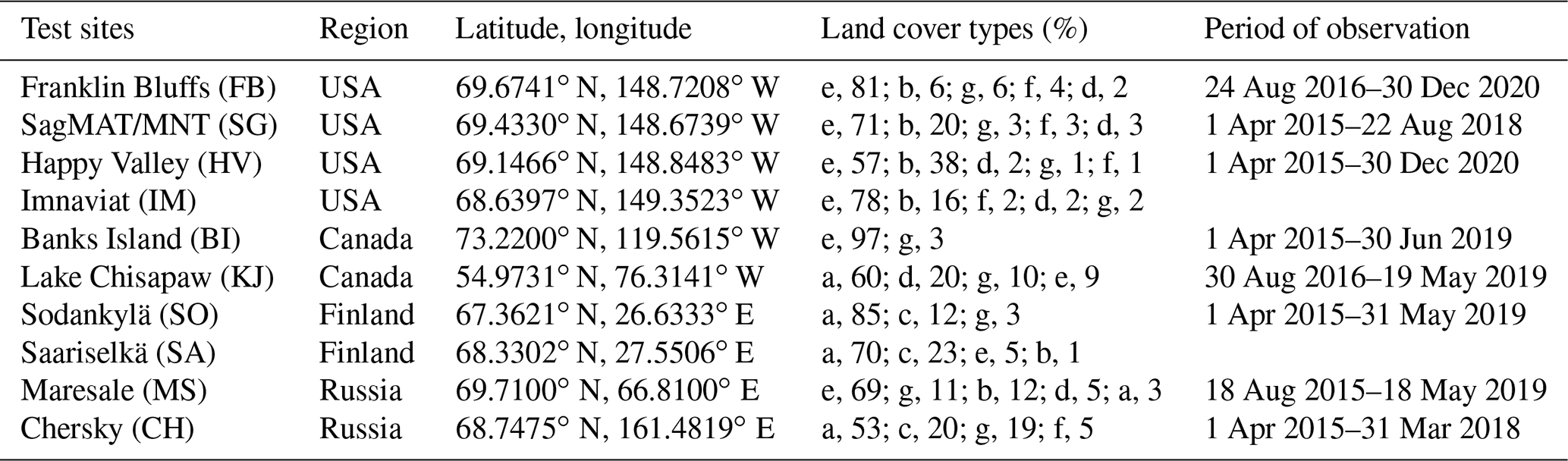
The abbreviations used in the table are as follows: a – forest; b – grassland; c – wetland; d – shrubland; e – sparse vegetation; f – bare area; g – water.
At the North Slope of Alaska test sites, soil temperature was measured at the surface (depth of 1 cm). The FB test site is located on a coastal plain on a flat alluvial terrace with a moss tundra landscape comprising moist nonacidic sedges and prostrate shrubs. The SG, HV and IM sites are located on hilly terrain with dominantly moist acidic and nonacidic tussock tundra to the north and considerable shrub growth to the south. The BI test site is characterized by gentle hills with sparse vegetation in the form of mosses and grassy meadows. Boreal forest test sites are represented by SO and SA in Finland and by KJ in Canada. The SO and SA sites are comprised of forests of differing densities, and non-forest area is covered with juniper, heather, and a thin layer of lichen and moss. KJ is located in typical Canadian taiga with a low-density black spruce–lichen woodland (sandy soils) landscape. The soil temperature at the SO, SA and KJ test sites was measured at a depth of 2–5 cm. The MS test site is located on the Yamal Peninsula in moist and dry dwarf shrub–moss–lichen tundra in combination with sedge–moss mires. The soil temperature at MS was measured at a depth of 2–5 cm. The CH area is dominated by wetlands covered with larch forests of varying canopy cover percentages (ranging from 13 % to 75 %). At the CH test site, the soil temperature was measured at five test plots (which were averaged for further analysis) at the interface between the organic and mineral soil layers, at depths of 6–10 cm below the surface depending on the organic layer thickness (Loranty and Alexander, 2021). At the KJ, MS and CH test sites, water objects occupied more than 10 % of the pixel area.
The brightness temperatures of the test sites were measured at vertical and horizontal polarizations by the SMAP and GCOM-W1 satellites at frequencies of 1.4 and of 6.9, 10.7, 18.7 and 36.5 GHz, respectively. Ascending SMAP and GCOM-W1 orbits were chosen. SMAP polarimetric brightness temperature data (SPL3FTP_E) for Northern Hemisphere azimuthal projections on a 9 km Equal-Area Scalable Earth Grid (EASE-Grid 2.0) were used over the test sites for the period of soil temperature observations by the weather stations (see Table 1). GCOM-W1 brightness temperature data were acquired from the L1R product, where the brightness temperatures of high-resolution channels are resampled to the effective pixel area of the lower-resolution channel at a frequency of 6.9 GHz, gridded with a 12.5 km cell size. Pixels closest to the coordinates of weather stations, with the exception of MS, were used in the analysis. MS is located at the coast of the Kara Sea; thus, a pixel whose center is far more than 50 km from the sea was chosen. The daily 9 km EASE-Grid freeze/thaw SMAP product (SPL3FTP_E, both ascending and descending orbits) based on the polarization index (Dunbar et al., 2016) was used for the identification of the FT state of land at the test sites.
The spectral components of brightness temperature are formed by the emitting layers of a ground half-space with different thicknesses. For this reason, the difference between brightness temperatures measured in the different parts of the frequency spectrum is related to the vertical (in the direction of the 0z axis) gradient of ground temperature Tg and, hence, to the direction of the heat flux , where K is the thermal conductivity, through the soil surface. Indeed, on the basis of the phenomenological theory of emission (Zuerndorfer and England, 1992), the brightness temperature ) of a dielectric half-space with a linear temperature profile can be represented as follows:
where f is the frequency electromagnetic field, Γp(f) is the ground reflectivity for vertical (p= V) or horizontal (p= H) polarization, Tg0 is the temperature of the ground surface, and zeff(f) is the thickness of emitting layer. From Eq. (1), it follows that the density of the spectral gradient of the brightness temperature is directly proportional to the heat flux through the boundary of the ground surface:
By analogy with the density of the spectral gradient of brightness temperature (Eq. 2), the density of the spectral gradient of reflectivity can be introduced: .
For a dielectric inhomogeneous and non-isothermal half-space, the reflectivity at frequency f, in accordance with the method of Muzalevskiy et al. (2021) and Muzalevskiy and Ruzicka (2020), can be estimated based on the following equation:
In Eq. (3), Teff and Γp(f) can be interpreted as the respective effective temperature and reflectivity of the layered structure of canopy and ground, which takes soil surface roughness and canopy optical thickness into account using one combined parameter (Fernandez-Moran et al., 2015, their Eq. 10). The effective temperature, Teff, can be estimated based on the measurements of brightness temperature, (6.9), by the GCOM-W1 satellite at a frequency of 6.9 GHz for vertical polarization, the values of which correlate with the surface temperature of tundra soil (Muzalevskiy et al., 2016). The physical basis for this estimate is the observation angle of AMSR-2/GCOM-W1, which is close to Brewster's angle (55∘), and this leads to a decreased impact of reflectivity, ΓV, on the measured brightness temperature, (6.9). Indeed, reflection coefficient measurements show that Brewster's angle decreases from 60 to 57∘ as root-mean-square (RMS) heights of soil surface roughness increase from 0.25 to 0.93 cm (De Roo and Ulaby, 1994; see also Wang et al., 1983, their Fig. 2). The roughness of natural tundra soils has much higher values, which vary over a wide range, from 1.06 to 4.28 cm (Watanabe et al., 2012). The presence of vegetation (snow) cover on a rough soil surface leads to blurring and flattening of the V polarization angular dependence of reflectivity (Rodriguez-Alvarez et al., 2011, their Figs. 7, 8) and brightness temperature (Lemmetyinen et al., 2016, their Figs. 5–7; Chang and Shiue, 1980, their Figs. 3–5) in the region of Brewster's angles, due to the interference phenomenon. Within the error measurement of brightness temperature of ±1.3–1.5 K (Piepmeier et al., 2017; Gao et al., 2019) as well as the accuracy of emission models of ±4–5 K (Wigneron et al., 2011), Brewster's angle can be determined within a wide range from about 45 to 65∘ (Lemmetyinen et al., 2016, their Figs. 5–7; Chang and Shiue, 1980, their Figs. 3–5). The error measurement of brightness temperature and the accuracy of emission models also make it possible to neglect the variations in H polarization brightness temperatures of snow- or vegetation-covered soil over a range of observation angles from 40 to 55∘ (Roy et al., 2018, their Fig. 3; Lemmetyinen et al., 2016, their Fig. 7; Chang and Shiue, 1980, their Figs. 3–5). In this regard, the use of brightness temperatures measured at different angles in Eq. (3) is approximate. As a result, and as expected from `Eq. (3), (6.9) becomes mainly directly proportional to Teff. For this reason, the reflectivity was further estimated only for horizontal polarization. Further, estimates of ΓH(f) will be considered to be the apparent values of reflectivity, as the absolute value of does not coincide with the actual values of Teff or Tg0 but is rather only proportional to them.
The time series of brightness temperatures, , measured by the SMAP and GCOM-W1 satellites, and the reflectivity, ΓH, calculated based on Eq. (3), are shown for the HV test site in Fig. 1a and b, respectively. For the other test sites, such dependencies are similar. The time series of and ΓH (see Fig. 1a and b, respectively) have a pronounced seasonal variation, with a periodic change in maximum and minimum values. On the dates corresponding to the moment of soil thawing or freezing, the order of brightness temperature and reflectivity values is inverted, along with an increase or decrease in frequency. Several such time periods are marked by dashed rectangles in Fig. 1a and b (see the period from 2015 to 2016).
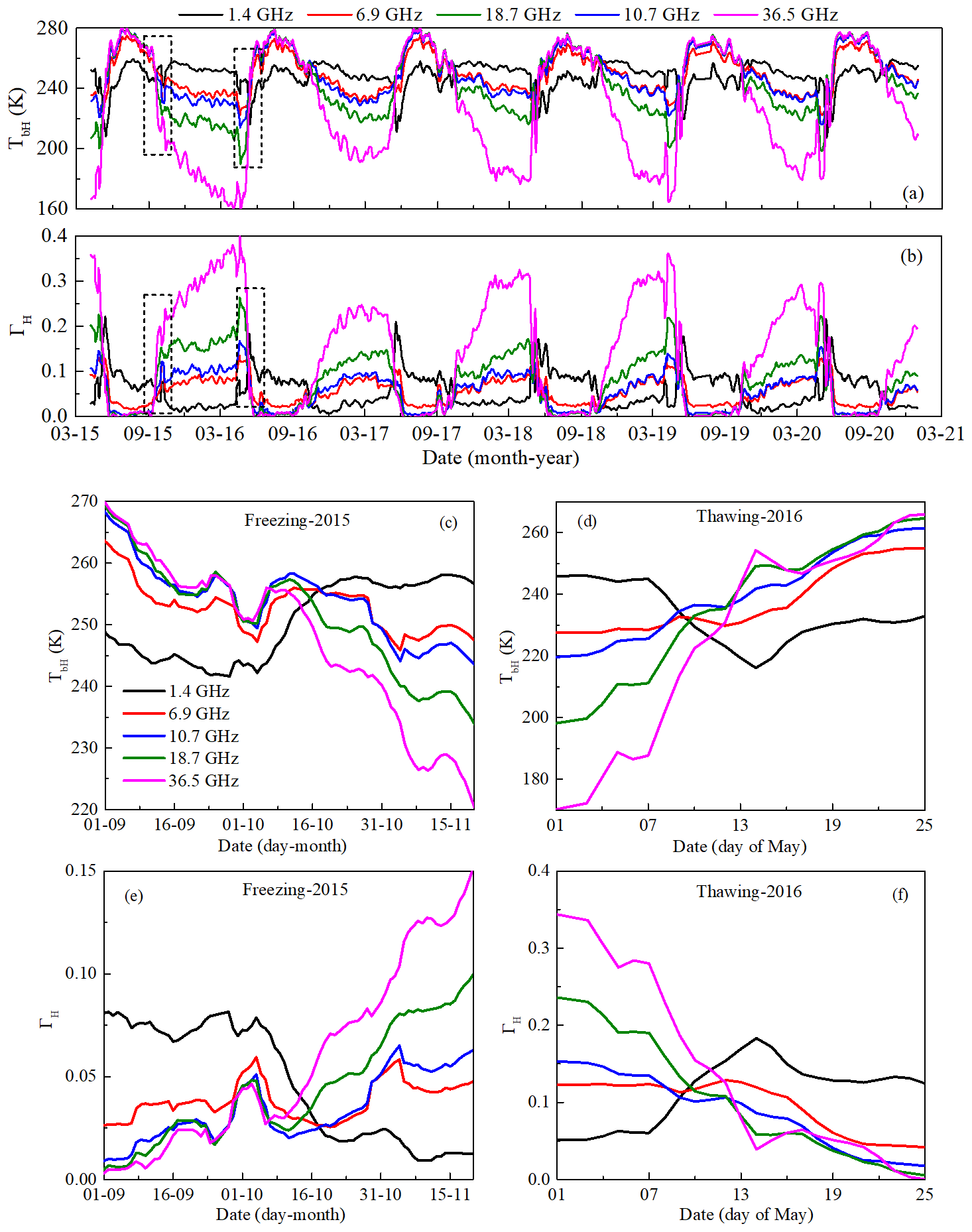
Figure 1Time series of brightness temperatures (a, c, d) and reflectivity (b, e, f) according to SMAP and GCOM-W1 satellite data in the frequency range from 1.4 to 36.5 GHz for the HV test site. Panels (c) and (e) show freezing process in 2015, whereas panels (d) and (f) present thawing process in 2016.
In Fig. 1, these areas are shown on a larger scale. Indeed, as can be seen from the aforementioned figure, the brightness temperature values decrease with increasing frequency in winter (before 7 May 2016 and after 1 November 2015), i.e., a negative gradient is observed, but a positive gradient is observed in summer (see Fig. 1c, d). The seasonal variation in reflectivity has an opposite spectral gradient (see Fig. 1e, f) with respect to the spectral gradient of brightness temperature. In the transition period (7–19 May 2016 and October–November 2015; see Fig. 1), the spectral gradient of brightness temperature and reflectivity is minimal. In these time intervals, for any pairs of and or ΓH(f1) and ΓH(f2) at different frequencies (f1 and f2), there is a point of zero spectral gradient (the point of sign change in the spectral gradient), at which the direction of the heat flux must change, in accordance with Eq. (2). Unlike the methods in which the FT index threshold level is set on the basis of calibration or normalization (Rautiainen et al., 2016; Derksen et al., 2017; Muzalevskiy and Ruzicka, 2020; Muzalevskiy et al., 2021), the zero-threshold level of spectral gradients of brightness temperatures or reflectivity does not require calibration for the identification of the FT topsoil state. FT classification based on the spectral gradient method was applied for the first time by Zuerndorfer et al. (1989).
Detailed depictions of the spectral gradient densities of brightness temperature and reflectivity are given in Fig. 2a and b, respectively, for the HV test site. To this end, the spectral gradient densities of brightness temperature and reflectivity were calculated for the following frequency ranges: 1.4–6.9, 1.4–10.7, 1.4–18.7 and 1.4–36.5 GHz. The largest variations in brightness temperatures ) and reflectivites ΔΓH(f) with frequency (see Fig. 1) are observed in winter, whereas the largest variations in the spectral gradient densities of brightness temperature (see Fig. 2a) and reflectivity (see Fig. 2b) are observed in summer. The spectral gradient of brightness temperature and reflectivity is highest in the frequency range of 1.4–36.5 GHz and lowest in the frequency range of 1.4–6.9 GHz. This is due to a significant contrast in temperatures and permittivities between the shallow and deeper emitting layers of the ground at frequencies of 36.5 and 1.4 GHz, respectively, compared with radiation layers that are close in thickness at frequencies of 1.4 and 6.9 GHz. At the same time, per unit interval of the frequency spectrum Δf, the spectral gradient densities of brightness temperature and reflectivity seem to be larger for the narrower (1.4–6.98 GHz) than for the wider (1.4–36.5 GHz) frequency band. The amplitudes of seasonal variations in are synchronous with variations in the surface temperature of soil. The time series of varies in antiphase with the soil surface temperature (see Fig. 2b). Figure 2 shows that the time points corresponding to the transitions in and through zero are well correlated with the time of the soil surface temperature Ts0 transition through 0 ∘C.
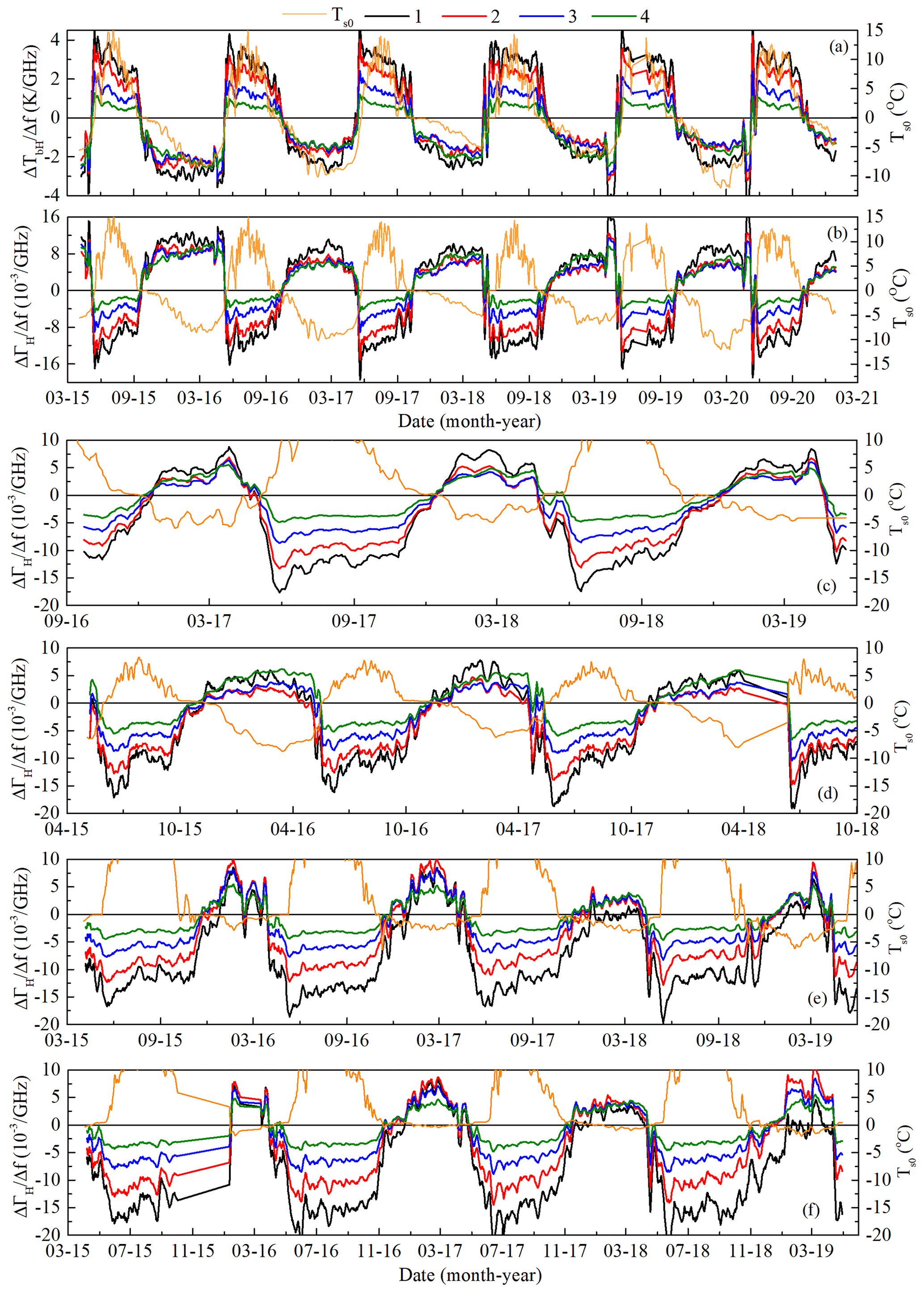
Figure 2The density of spectral gradients of brightness temperature (a) and reflectivity (b) for the HV test site and the density of spectral gradients of reflectivity for the (c) KJ, (d) CH, (e) SO and (f) SA test sites, calculated for the following pairs of frequencies: (1) 1.4–6.9 GHz, (2) 1.4–10.7 GHz, (3) 1.4–18.7 GHz and (4) 1.4–36.5 GHz.
Similar patterns in the behavior of and are also observed for other test sites, except for SO and SA. As an example, for the KJ, CH, SO and SA test sites are shown in Fig. 2c, d, e and f, respectively. In some years, multiple passing of through zero during winter can be observed for the SO and SA test sites (see Fig. 2e and f, respectively), which does not allow for unambiguous identification of the FT states. These processes will be explained below. Moreover, it should be noted that the presence of significant wetland or open water at the CH test site is not detected in the behavior of (), in comparison with other test sites.
For further analysis, seasonal variations in and will be used, the amplitudes of which take maximum (see Fig. 2, curve 1) and minimum (see Fig. 2, curve 4) values in the frequency ranges of 1.4–36.5 and 1.4–6.9 GHz, respectively. The soil will be considered frozen or thawed when the soil surface temperature, Ts0, transits through 0 ∘C, according to weather stations installed at the test sites.
The synchronicity of the transition through the zero spectral gradient density threshold of brightness temperature and reflectivity with the soil surface temperature crossing 0 ∘C was estimated (see Fig. 3).
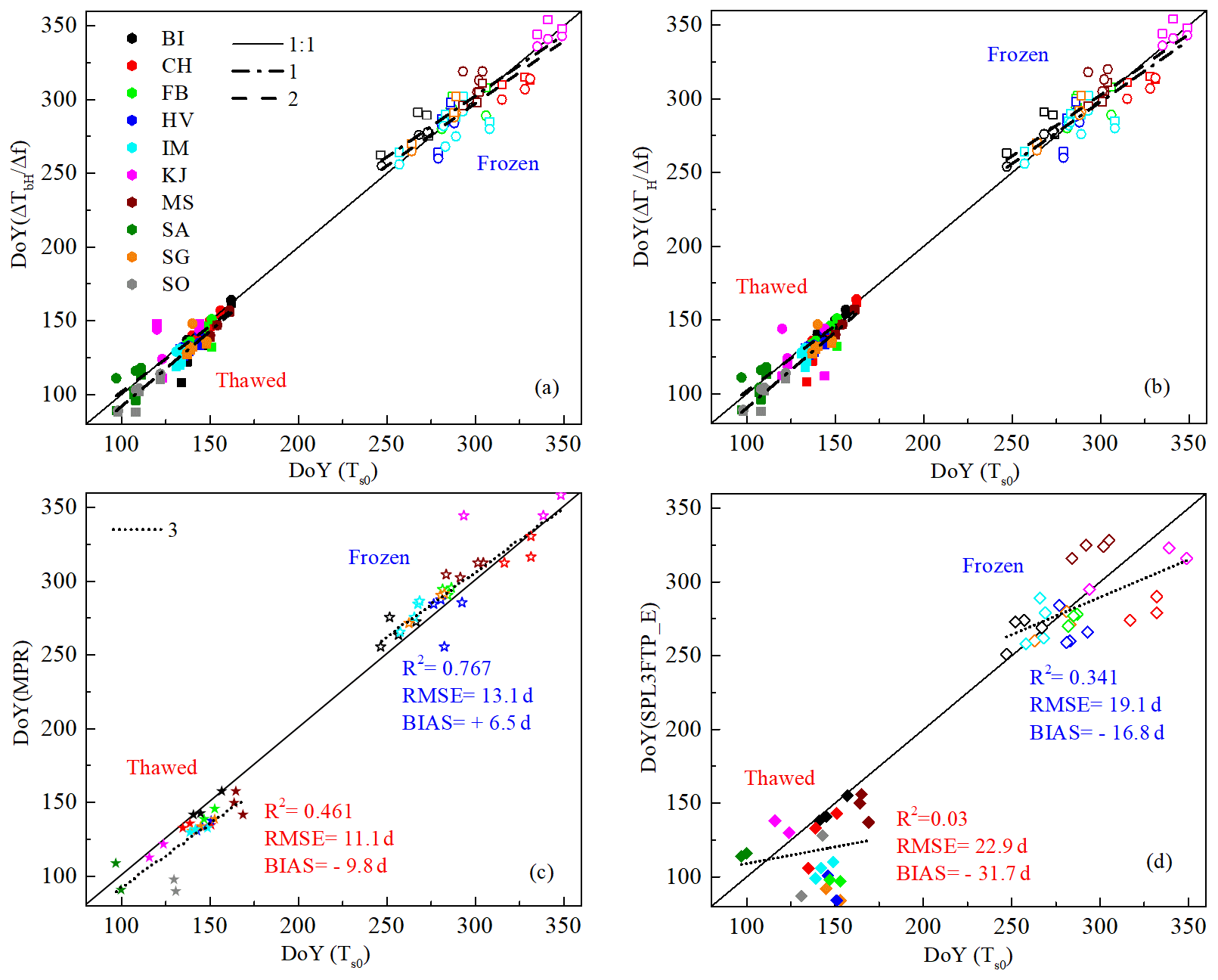
Figure 3Correlation between the day of the year (DoY) on which (a), (b) or MPR (c) crosses the threshold level and the stable soil surface temperature crossing 0 ∘C; correlation between the DoY on which (d) soil becomes FT based on the SMAP SPL3FTP_E product and the stable soil surface temperature crossing 0 ∘C. Different test sites are distinguished using different colors. The open and filled symbols indicate the frozen and thawed topsoil state, respectively. Squares and circles indicated a spectral range of 6.9–1.4 and 36.5–1.4 GHz, respectively. Regression lines for the spectral ranges of 6.9–1.4 and 36.5–1.4 GHz are marked as (1) and (2), respectively. Regression line (3) corresponds to the MPR index and the SMAP SPL3FTP_E product.
From the correlation analysis of the data presented in Fig. 3, it follows that the () in the frequency range of 6.9–1.4 GHz (36.5–1.4 GHz) determines the thawed state of the topsoil 8.4–8.9 (1.2–3.3) d earlier, relative to soil surface temperature (see the bias estimations in Table 2).
Table 2Determination coefficient (R2), root-mean-square error (RMSE) and bias in identifying the FT topsoil state.
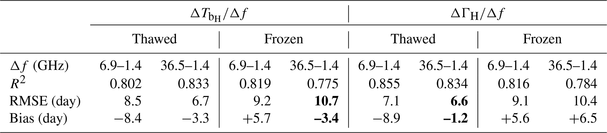
In the frequency range of 6.9–1.4 GHz, the frozen topsoil state is determined 5.6–5.7 d later on average (see both indexes in Table 2). In the frequency range of 36.5–1.4 GHz, makes it possible to determine the frozen topsoil state 3.4 d earlier (see bias in Table 2); in the frequency range of 6.9–1.4 GHz, makes it possible to determine the frozen topsoil state 6.5 d later (see bias in Table 2). In general, both indexes, and , have similar RMSE values with respect to predicting the FT topsoil state. At the same time, for the identification of a thawed topsoil state, has a greater accuracy (bias and RMSE are lower and R2 is higher compared with ; see Table 2) in the spectral range of 36.5–1.4 GHz. is more suitable for identifying a frozen topsoil state in the frequency range of 36.5–1.4 GHz (see Table 2), as it has a smaller bias (at comparable RMSE and R2 values) compared with . Spectral gradient methods have improved accuracy with respect to identifying the FT topsoil state in relation to both the MPR index (see Fig. 3c and the bold information in Table 2) and the standard SMAP product SPL3FTP_E (see Fig. 3d and the bold information in Table 2).
It should be noted that the correlation analysis (in the case of the frozen state) did not take the SO and SA test sites into account, as the and indexes led to a systematic error of about 1.5 months, due to unstable soil freezing (soil surface temperature for most of the winter ranged from from 0 to between −2 and −5 ∘C according to weather stations; see Fig. 2f and e). This systematic error may be because, in contrast to the other test sites, SO and SA stand out with the largest share of forest, from 70 % to 85 %, in the footprint (see Table 1). Apparently, such a significant share of forest contributes to the formation of a thicker forest litter layer and increased accumulation of snow cover compared with the rest of the test sites (e.g. sites KJ and CH, in which the share of forest is less than 60 % and 53 %, respectively). Thicker forest litter and snow cover create additional inertia in the thermal exchange between air and soil. Indeed, according to data from the SO and SA stations, these test sites have low negative soil surface temperatures in winter as well as an extended period of zero-curtain effect (see Fig. 2e and f for SO and SA, respectively). As a result, in some years, the unstable FT transition state of topsoil is reflected in the unstable transition of () through zero during winter, which explains the observed systematic error for the SO and SA test sites. Similar unstable transitions of brightness temperature have been observed in ground-based radiometric experiments at the SO test site (Lemmetyinen et al., 2016, their Fig. 2 “wetland 2013–2014”); thawed soil under a dry snow layer is a common phenomenon (Kumawat et al., 2022).
In this article, spectral gradient methods were used to identify the FT topsoil state of northern regions based on brightness temperature measurements from the SMAP and GCOM-W1 satellites across a wide frequency range. As criteria for determining the FT topsoil state, the spectral gradient densities of brightness temperature and reflectivity were used in the frequency range from 1.4 to 6.9 GHz and from 1.4 to 36.5 GHz. Both criteria give a comparable accuracy with respect to forecasting the FT topsoil state for tundra and boreal forest regions. However, the spectral gradient density of reflectivity should be used to improve the accuracy of thawed topsoil state predictions, whereas the spectral gradient density of brightness temperature (the frequency range of 1.4–36.5 GHz) should be used for identification of frozen topsoil state. The proposed method makes it possible to identify forest soils that are in a transitional state (the soil surface temperature is about 0 ∘C or has small negative values), which is revealed in the multiple transitions of spectral gradient densities of brightness temperature and reflectivity through zero (more pronounced in the frequency range of 1.4–6.9 GHz). The methods considered in this work do not fully separate the contributions of the FT topsoil state from those of waterbodies. The freezing processes of open-water areas with the formation of ice, the description of which requires a large number of additional data on snow cover thickness, air and water temperature, and wind speed are particularly difficult to account for. We did not find any significant differences in the behavior of the spectral gradient densities of brightness temperature and reflectivity measured for the test site with a high share of wetland (20 %) and open water (19 %) compared with the other test sites. Despite all assumptions made in the proposed method, the identification of FT soil surface states is possible with a relatively high determination coefficient of 0.775–0.834, a small root-mean-square error of 6.6–10.7 d, and a bias from −3.4 to +6.5 d. Further validation of this methodology, requires expanding the number of test sites, as the current analysis is limited by the small number of soil–climatic weather stations with available and up-to-date soil active-layer temperature data.
SMAP data are available from https://doi.org/10.5067/XB8K63YM4U8O (Chaubell et al., 2020). GCOM-W1 data are available from https://gportal.jaxa.jp/gpr/?lang=en (last accessL 15 September 2023, Maeda et al., 2016). Geospatial data for land cover are available from https://www.esa-landcover-cci.org/ (last access: 15 September 2023, Harper et al., 2023). Soil temperature data over Alaska test sites are available from https://permafrost.gi.alaska.edu/sites_map (Permafrost Laboratory Geophysical Institute, the University of Alaska Fairbanks, 2023).
KM designed the study, performed the analyses and prepared the manuscript. ZR supported the satellite data processing. AR, ML and AV supported the ground truth data processing. All authors contributed to writing the manuscript and discussing the results.
The contact author has declared that none of the authors has any competing interests.
Publisher's note: Copernicus Publications remains neutral with regard to jurisdictional claims in published maps and institutional affiliations.
The authors express their sincere gratitude to the anonymous referees for their comments, which improved the quality of this article, and for the opportunity to publish this article. We are also grateful to the Colgate University Research Council for support.
This research has been supported by the state assignment of the Kirensky Institute of Physics, Federal Research Center, Krasnoyarsk Science Center of the Siberian Branch of the Russian Academy of Sciences (SB RAS). Weather station data collection was support by the Canadian Space Agency, NSERC and frqnt; the US National Science Foundation (PLR-1304464 and PLR-1417745); and the state assignment of the Earth Cryosphere Institute, Tyumen Scientific Centre, SB RAS (121041600043-4). Publisher’s note: the article processing charges for this publication were not paid by a Russian or Belarusian institution.
This paper was edited by Christian Beer and reviewed by two anonymous referees.
Chang, A. T. C. and Shiue, J. C.: A comparative study of microwave radiometer observations over snowfields with radiative transfer model calculations, Remote Sens. Environ., 10, 215–229, https://doi.org/10.1016/0034-4257(80)90025-5, 1980.
Chaubell, J., Chan, S., Dunbar, R. S., Peng, J., and Yueh, S.: SMAP Enhanced L1C Radiometer Half-Orbit 9 km EASE-Grid Brightness Temperatures, Version 3, Boulder, Colorado, USA NASA National Snow and Ice Data Center [data set], https://doi.org/10.5067/XB8K63YM4U8O, 2020.
Derksen, C., Xu, X., Dunbar, R. S., Colliander, A., Kim, Y., Kimball, J. S., Black, T. A., Euskirchen, E., Langlois, A., Loranty, M.M., Marsh, P., Rautiainen, K., Roy, A., Royer, A., and Stephens, J.: Retrieving Landscape Freeze/Thaw State from Soil Moisture Active Passive (SMAP) Radar and Radiometer Measurements, Remote Sens. Environ., 194, 48–62, https://doi.org/10.1016/j.rse.2017.03.007, 2017.
De Roo, R. D. and Ulaby, F. T.: Bistatic specular scattering from rough dielectric surfaces, IEEE T. Antenn. Propag., 42, 220–231, https://doi.org/10.1109/8.277216, 1994.
Dunbar, S., Xu, X., Colliander, A., Derksen, C., Kimball, J., and Kim, Y.: Algorithm Theoretical Basis Document (ATBD), SMAP Level 3 Radiometer Freeze/Thaw Data Products, JPL CIT: JPL D-56288, 33, https://smap.jpl.nasa.gov/system/internal_resources/details/original/274_L3_FT_A_RevA_web.pdf (last access: 15 September 2023), 2016.
ESA: Land Cover CCI Product User Guide Version 2, Tech. Rep., http://maps.elie.ucl.ac.be/CCI/viewer/download/ESACCI-LC-Ph2-PUGv2_2.0.pdf (last access: 15 September 2023), 2017.
Fernandez-Moran, R., Wigneron, J.-P., Lopez-Baeza, E., Al-Yaari, A., Coll-Pajaron, A., Mialon, A., Miernecki, M., Parrens, M., Salgado-Hernanz, P. M., Schwank, M., Wang, S., and Kerr, Y. H.: Roughness and vegetation parameterizations at L-band for soil moisture retrievals over a vineyard field, Remote Sens. Environ., 170, 269–279, https://doi.org/10.1016/j.rse.2015.09.006, 2015.
Fisher, R. A.: The use of multiple measurements in taxonomic problem, Ann. Eugenic., 7, 179–188, https://doi.org/10.1111/j.1469-1809.1936.tb02137.x, 1936.
Gao, S., Li, Z., Chen, Q., Zhou, W., Lin, M., and Yin, X.: Inter-Sensor Calibration between HY-2B and AMSR2 Passive Microwave Data in Land Surface and First Result for Snow Water Equivalent Retrieval, Sensors, 19, 5023, https://doi.org/10.3390/s19225023, 2019.
Harper, K. L., Lamarche, C., Hartley, A., Peylin, P., Ottlé, C., Bastrikov, V., San Martín, R., Bohnenstengel, S. I., Kirches, G., Boettcher, M., Shevchuk, R., Brockmann, C., and Defourny, P.: A 29-year time series of annual 300 m resolution plant-functional-type maps for climate models, Earth Syst. Sci. Data, 15, 1465–1499, https://doi.org/10.5194/essd-15-1465-2023, 2023.
Hu, T., Zhao, T., Shi, J., Wu, S., Liu, D., Qin, H., and Zhao, K.: High-Resolution Mapping of Freeze/Thaw Status in China via Fusion of MODIS and AMSR2 Data, Remote Sens.-Basel, 9, 1339, https://doi.org/10.3390/rs9121339, 2017.
Hu, T., Zhao, T., Zhao, K., and Shi, J.: A continuous global record of near-surface soil freeze/thaw status from AMSR-E and AMSR2 data, Int. J. Remote Sens., 40, 6993–7016, https://doi.org/10.1080/01431161.2019.1597307, 2019.
Kilic, L., Prigent, C., Jimenez, C., and Donlon, C.: Technical note: A sensitivity analysis from 1 to 40 GHz for observing the Arctic Ocean with the Copernicus Imaging Microwave Radiometer, Ocean Sci., 17, 455–461, https://doi.org/10.5194/os-17-455-2021, 2021.
Kumawat, D., Olyaei, M., Gao, L., and Ebtehaj, A.: Passive Microwave Retrieval of Soil Moisture Below Snowpack at L-Band Using SMAP Observations, IEEE T. Geosci. Remote, 60, 4415216, https://doi.org/10.1109/TGRS.2022.3216324, 2022.
Lemmetyinen, J., Schwank, M., Rautiainen, K., Kontu, A., Parkkinen, T., Mätzler, C., Wiesmann, A., Wegmüller, U., Derksen, C., Toose, P., Roy, A., and Pulliainen, J.: Snow density and ground permittivity retrieved from L-band radiometry: application to experimental data, Remote Sens. Environ., 180, 377–391, https://doi.org/10.1016/j.rse.2016.02.002, 2016.
Loranty, M. M. and Alexander, H. D.: Understory micrometorology across a larch forest density gradient in northeastern Siberia 2014–2020, Arctic Data Center [data set], https://doi.org/10.18739/A24B2X59C, 2021.
Maeda, T., Taniguchi, Y., and Imaoka, K.: GCOM-W1 AMSR2 Level 1R Product: Dataset of Brightness Temperature Modified Using the Antenna Pattern Matching Technique, IEEE T. Geosci. Remote, 54, 770–782, https://doi.org/10.1109/TGRS.2015.2465170, 2016.
Muzalevskiy, K. and Ruzicka, Z.: Detection of Soil Freeze/Thaw States in the Arctic Region Based on Combined SMAP and AMSR-2 Radio Brightness Observations, Int. J. Remote Sens., 41, 5046–5061, https://doi.org/10.1080/01431161.2020.1724348, 2020.
Muzalevskiy, K., Ruzicka, Z., Roy, A., Loranty, M., and Vasiliev, A.: Classification of the frozen/thawed surface state of Northern land areas based on SMAP and GCOM-W1 brightness temperature observations at 1.4 GHz and 6.9 GHz, Remote Sens. Lett., 11, 1073–1081, https://doi.org/10.1080/2150704X.2021.1963497, 2021.
Muzalevskiy, K. V., Ruzicka, Z., Kosolapova, L. G., and Mironov, V. L.: Temperature dependence of SMOS/MIRAS, GCOM-W1/AMSR2 brightness temperature and ALOS/PALSAR radar backscattering at arctic test sites, Proceedings of Progress in Electromagnetic Research Symposium (PIERS), Shanghai, 3578–3582, https://doi.org/10.1109/PIERS.2016.7735375, 2016.
Permafrost Laboratory Geophysical Institute, the University of Alaska Fairbanks: Permafrost Laboratory, https://permafrost.gi.alaska.edu/sites_map, last access: 15 September 2023.
Piepmeier, J. R., Focardi, P., Horgan, K. A., Knuble, J., Ehsan, N., Lucey, J., Brambora, C., Brown, P. R., Hoffman, P. J., French, R. T., Mikhaylov, R. L., Kwack, E. Y., Slimko, E. M., Dawson, D. E., Hudson, D., Peng, J., Mohammed, P. N., De Amici, G., Freedman, A. P., Medeiros, J., Sacks, F., Estep, R., Spencer, M. W., Chen, C. W., Wheeler, K. B., Edelstein, W. N., O'Neill, P. E., and Njoku, E. G.: SMAP L-Band Microwave Radiometer: Instrument Design and First Year on Orbit, IEEE T. Geosci. Remote, 55, 1954–1966, https://doi.org/10.1109/tgrs.2016.2631978, 2017.
Rautiainen, K., Lemmetyinen, J., Schwank, M., Kontu, A., Ménard, C., Mätzler, C., Drusch, M., Wiesmann, A., Ikonen, J., and Pulliainen, J.: Detection of soil freezing from L-band passive microwave observations, Remote Sens. Environ., 147, 206–218, https://doi.org/10.1016/j.rse.2014.03.007, 2014.
Rautiainen, K., Parkkinen, T., Lemmetyinen, J., Schwank, M., Wiesmann, A., Ikonen, J., Derksen, C., Davydov, S., Davydova, A., Boike, J., Langer, M., Drusch, M., and Pulliainen, J.: SMOS prototype algorithm for detecting autumn soil freezing, Remote Sens. Environ., 180, 346–360, https://doi.org/10.1016/j.rse.2016.01.012, 2016.
Rodriguez-Alvarez, N., Camps, A., Vall-llossera, M., Bosch-Lluis, X., Monerris, A., Ramos-Perez, I., and Sanchez, N.: Land Geophysical Parameters Retrieval Using the Interference Pattern GNSS-R Technique, IEEE T. Geosci. Remote, 49, 71–84, https://doi.org/10.1109/TGRS.2010.2049023, 2011.
Roy, A., Royer, A., Derksen, C., Brucker, L., Langlois, A., Mialon, A., and Kerr, Y.: Evaluation of spaceborne L-band radiometer measurements for terrestrial freeze/thaw retrievals in Canada, IEEE J. Sel. Top. Appl., 8, 4442–4459, https://doi.org/10.1109/JSTARS.2015.2476358, 2015.
Wang, J. R., O'Neill, P. E., Jackson, T. J., and Engman, E. T.: Multifrequency Measurements of the Effects of Soil Moisture, Soil Texture, And Surface Roughness, IEEE T. Geosci. Remote, 21, 44–51, https://doi.org/10.1109/TGRS.1983.350529, 1983.
Watanabe, M., Kadosaki, G., Kim, Y., Ishikawa, M., Kushida, K., Sawada, Y., Tadono, T., Fukuda, M., and Sato, M.: Analysis of the Sources of Variation in L-band Backscatter From Terrains With Permafrost, IEEE T. Geosci. Remote, 50, 44–54, https://doi.org/10.1109/TGRS.2011.2159843, 2012.
Wigneron J.-P., Chanzy, A., Kerr, Y., Lawrence, H., Shi, J., Escorihuela, M. J., Mironov, V., Mialon, A., Demontoux, F., de Rosnay, P., and Saleh-Contell, K.: Evaluating an Improved Parameterization of the Soil Emission in L-MEB, IEEE T. Geosci. Remote, 49, 1177–1189, https://doi.org/10.1109/TGRS.2010.2075935, 2011.
Zhao, T., Zhang, L., Jiang, L., Zhao, S., Chai, L., and Jin, R.: A new soil freeze/thaw discriminant algorithm using AMSR-E passive microwave imagery, Hydrol. Process., 25, 1704–1716, https://doi.org/10.1002/hyp.7930, 2011.
Zhao, T., Shi, J., Hu, T., Zhao, L., Zou, D., Wang, T., Ji, D., Li, R., and Wang, P.: Estimation of high-resolution near surface freeze/thaw state by the integration of microwave and thermal infrared remote sensing data on the Tibetan Plateau, Earth Space Sci., 4, 472–484, https://doi.org/10.1002/2017EA000277, 2017.
Zuerndorfer, B. and England, A. W., Radiobrightness decision criteria for freeze/thaw boundaries, IEEE T. Geosci. Remote, 30, 89–102, https://doi.org/10.1109/36.124219, 1992.
Zuerndorfer, B. W., England, A. W., Dobson, M. C., and Ulaby, F. T.: Mapping freeze/thaw boundaries with SMMR data, NASA Contractor Report 184991, 28, https://ntrs.nasa.gov/citations/19890014590 (last access: 15 September 2023), 1989.
Zuerndorfer, B. W., England, A. W., Dobson, M. C., and Ulaby, F. T.: Mapping freeze/thaw boundaries with SMMR data, Agr. Forest Meteorol., 52, 199–225, 1990.
- Abstract
- Introduction
- Test sites, the ground truth and satellite data
- Spectral gradient methods for identifying the frozen/thawed state of topsoil
- Results and discussion
- Conclusions
- Data availability
- Author contributions
- Competing interests
- Disclaimer
- Acknowledgements
- Financial support
- Review statement
- References