the Creative Commons Attribution 4.0 License.
the Creative Commons Attribution 4.0 License.
 | 06 Sep 2023
Relevance of warm air intrusions for Arctic satellite sea ice concentration time series
Philip Rostosky
Gunnar Spreen
Winter warm air intrusions entering the Arctic region can strongly modify the microwave emission of the snow-covered sea ice system due to temperature-induced snow metamorphism and ice crust formations, e.g., after melt–refreeze events. Common microwave radiometer satellite sea ice concentration retrievals are based on empirical models using the snow-covered sea ice emissivity and thus can be influenced by strong warm air intrusions. Here, we carry out a long-term study analyzing 41 years of winter sea ice concentration observations from different algorithms to investigate the impact of warm air intrusions on the retrieved ice concentration. Our results show that three out of four algorithms underestimate the sea ice concentration during (and up to 10 d after) warm air intrusions which increase the 2 m air temperature (daily maximum) above − 5 ∘C. This can lead to sea ice area underestimations in the order of 104 to 105 km2. If the 2 m temperature during the warm air intrusions crosses − 2 ∘C, all algorithms are impacted. Our analysis shows that the strength of these strong warm air intrusions increased in recent years, especially in April. With a further climate change, such warm air intrusions are expected to occur more frequently and earlier in the season, and their influence on sea ice climate data records will become more important.
- Article
(7034 KB) - Full-text XML
- BibTeX
- EndNote


Sea ice concentration estimates from passive microwave satellite observations are an important dataset for observing and understanding the Arctic climate system and for monitoring its recent drastic changes (e.g., Perovich et al., 2017; Maslanik et al., 2011; Kumar et al., 2010). Long-term, inter-calibrated sea ice concentration datasets provided by, e.g., the National Snow and Ice Data Center (NSIDC) (Meier et al., 2021) and the Ocean and Sea Ice Satellite Application Facility (OSI SAF) (Lavergne et al., 2016, 2019) are of special value since they provide consistent, more than 40 year long, time series of Arctic sea ice cover. They naturally have a rather coarse spatial resolution in the order of 25 km2. Methods like the ARTIST Sea Ice (ASI) algorithm (Spreen et al., 2008) utilize observations at a higher microwave frequency at 89 GHz (available since 2002 for AMSR-E/2), which has a higher spatial resolution (6.25 km2 grid resolution for AMSR-E/2).
Even after decades of research, accurate estimation of sea ice concentration and thus sea ice area remains challenging, especially in summer (Ivanova et al., 2015; Kern et al., 2019, 2020, 2022; Liu and Curry, 2003; Tonboe et al., 2003, e.g.,). In winter and spring, atmospheric warm air intrusions, which increased in intensity and frequency in recent years (Graham et al., 2017), can influence not only the sea ice conditions due to dynamic and thermodynamic processes (Aue et al., 2022; Clancy et al., 2021; Graham et al., 2019b) but also the microwave signal of the snow-covered sea ice system due to rapid snow metamorphism and melt–refreeze events (Comiso et al., 1997; Drinkwater et al., 1995; Kern et al., 2020; Rückert et al., 2023; Tonboe et al., 2003). Of importance is that the impact of snow warming, snow metamorphism and snow surface changes due to melt–refreeze events can be visible in the microwave signal for several days and up to weeks after the event (e.g., Rückert et al., 2023). Consequently, warm air intrusions can impact the quality of satellite sea ice concentration retrievals. Rückert et al. (2023) investigated the impact of such a warm air intrusion along the MOSAiC (Multidisciplinary Drifting Observatory of the Study of Arctic Climate) campaign in the central Arctic in April 2020 and found a strong drop in retrieved ice concentration caused by the formation of a large-scale glazed ice layer on top of the snow.
The aim of this study is to analyze (I) how strong the impact of winter warm air intrusions on the retrieved sea ice concentration is and (II) whether the impact increased in recent years due to an increase in frequency of strong warm air intrusions entering the Arctic region. We hereby analyze four common sea ice products: the National Snow and Ice Data Center (NSIDC) (Meier et al., 2021, version 4) and Ocean and Sea Ice Application Facility (OSI SAF) (Lavergne et al., 2016, 2019, version 3) climate data records (CDRs), as well as the ASI (Spreen et al., 2008) and the NASA-Team (used here is the product provided within the NSIDC CDR) sea ice concentration algorithms.
The article is organized as follows. In Sect. 2, the basics of passive microwave sea ice concentration algorithms are briefly introduced, and the datasets used in this study are described. The method to detect and define warm air intrusions is described in Sect. 3. In Sect. 4, the main results are presented, and in Sect. 5, the uncertainty and possible error sources of the results are discussed. In addition, a detailed discussion of the performance of the NSIDC and OSI SAF CDR products is provided. The article closes with a conclusion.
Passive microwave satellite sensors are a common tool to observe the sea ice in the Arctic and Antarctic oceans. To the first order, sea ice concentration algorithms take advantage of the strong emissivity difference between sea ice (ϵ>0.8, depending on the frequency) and sea water (ϵ<0.3), which make the two surfaces easily distinguishable. In addition, the polarization difference and emissivity changes with frequency can be used to distinguish ice and water. Different algorithms use different methods and frequencies to relate the observed emissivity to sea ice concentration.
In general, the emissivity of sea ice depends on the physical quantities of the ice and snow as well as on the microwave frequency. In Spreen et al. (2008), Fig. 1, the typical emissivity of different surface types (first-year ice, multiyear ice and open ocean) are shown as a function of typical microwave frequencies used by satellites and most of the common sea ice concentration retrievals. However, the emissivity of the snow-covered sea ice system depends on many parameters. The main drivers are snow and ice temperature, ice type and the snow microstructure. Ice layers within or ice crusts at top of the snowpack can influence sea ice concentration retrievals that use polarization differences or ratios (due to their strong impact on horizontal polarization; Comiso et al., 1997; Mätzler et al., 1984). At frequencies higher than 19 GHz, parameters like snow grain size and shape also become important influences for, e.g, retrievals that use gradient ratios of two different frequencies.
Several studies have shown that strong weather events like warm air intrusions, introducing snow metamorphism, melt–refreeze events or liquid water formation in the snow modify the above-mentioned parameters and consequently influence the emissivity of the snow-covered sea ice system (e.g., Liu and Curry, 2003; Rückert et al., 2023; Stroeve et al., 2022; Tonboe et al., 2003). Therefore, warm air intrusions can introduce false changes in the retrieved sea ice concentration (e.g., Tonboe et al., 2003).
Figure A3 (Fig. 4 from Rückert et al., 2023) in the Appendix shows the temporal evolution of brightness temperatures and derived parameters for a warm air intrusion in April 2020. A strong impact on the brightness temperatures at higher frequencies (19–89 GHz) is visible during the events, while the polarization difference and ratio (which are used in the sea ice retrievals analyzed in this study) show a strong increase just after the warming events due the formation of a large-scale glazed ice layer on top of the snow. The gradient ratio shows a strong increase during the events. It remains higher after the event, indicating that snow metamorphism led to stronger scatter, influencing the higher frequencies. In this study, as already mentioned, four different sea ice concentration products are analyzed. The Ocean and Sea Ice Satellite Application Facility (OSI SAF) (Lavergne et al., 2016, 2019) and National Snow and Ice Data Center (NSIDC) (Meier et al., 2021) algorithms are so-called climate data records (CDRs). CDRs are designed to provide consistent, reproducible long-term time series of climate variables. Long-term sea ice concentration is also provided by, e.g., the NASA-Team algorithm (Cavalieri et al., 1997), which is frequently used and is part of the NSIDC CDR. All these retrievals utilize microwave frequencies between 6.9 and 36.5 GHz. Additionally, we analyze the performance of the ASI algorithm (Spreen et al., 2008), which is based on 89 GHz. All algorithms are re-sampled to a 25 × 25 km2 polar stereographic grid which is the resolution of the coarsest product.
2.1 NSIDC climate data record
More than 40 years of consistent sea ice concentration observations from various satellites are provided by the NSIDC (Meier et al., 2021, version 4). Daily sea ice concentration is estimated by combining two different products, i.e., the NASA-Team (Cavalieri et al., 1997) and Bootstrap (Comiso, 1986) algorithms. For the final product, the higher sea ice concentration of the two sub-algorithms is used on a grid cell level. The sub-algorithms are based on brightness temperature observations at 19 and 37 GHz at polarizations both horizontal (H) and vertical (V). The Bootstrap algorithm uses dynamic (daily) tie points to mitigate the impact of brightness temperature variability (Comiso et al., 2017). A full description of the product can be found at https://nsidc.org/data/g02202/versions/4 (last access: 20 March 2023). The resolution of this product is 25×25 km2. An uncertainty estimation is given for an individual grid cell based on the spatial variability within the nine surrounding grid cells of both sub-algorithms.
2.2 OSI SAF climate data record
OSI SAF provides daily sea ice concentration based on a dynamic algorithm (Lavergne et al., 2016, 2019). Brightness temperatures at 19 V, 37 V and 37 H are used to estimate daily sea ice concentration values at 25×25 km2 resolution. OSI SAF includes ERA5 reanalysis data for correcting atmospheric effects on the brightness temperature observations. The uncertainty in sea ice concentration is estimated by combining the uncertainty of the algorithm itself and the “smearing” uncertainty due to the daily gridding of several orbits for the final product. A full description of the product is provided at https://osi-saf.eumetsat.int/products/osi-450-a (last access: 12 July 2023). The reference to the dataset is osi-450-a (OSI, 2023).
2.3 ASI
The ASI algorithm estimates the sea ice concentration from passive microwave satellite observations from AMSR-E and AMSR2 at 89 GHz. It is based on a empirical equation relating the polarization difference (i.e., brightness temperatures at V-Pol − H-Pol) to sea ice concentration (Spreen et al., 2008). The spatial resolution of this product is 6.25×6.25 km2 Additional weather filters using lower frequencies are applied to reduce the impact of clouds and water vapor over the open ocean on the retrieved ice concentration. The uncertainty is dependent on the ice concentration and is around 5% in the high ice concentration regime.
2.4 NASA-Team
The NASA-Team ice concentration algorithm (Cavalieri et al., 1997) is provided within the NSIDC CDR dataset. It is based on a combination of the polarization ratio at 19 GHz and the gradient ratio of 37 and 19 GHz (V polarization). No additional uncertainty estimation for the NASA-Team sub-algorithm is provided.
2.5 ERA5
In this study, 2 m air temperature from ERA5 (Hersbach et al., 2020) reanalysis data are used to detect warm air intrusions. Here the daily maximum of the temperature is used (referred to as daily max., hereafter). ERA5 is known to have a positive temperature bias in the Arctic (Batrak and Müller, 2019; Herrmannsdörfer et al., 2023; Wang et al., 2019). Possible consequences are discussed in Sect. 5.1.
3.1 Overview of procedure
Here, we describe the algorithm used in this study. The algorithm is built to detect connected areas where the daily max. 2 m air temperature (from ERA5; Hersbach et al., 2020) crosses a certain threshold within a given time window.
An overview of the procedure of the algorithm to detect warm air intrusions is given in Fig. 1. The input for the detection algorithm are 30 d arrays of gridded ERA5 daily max. 2 m air temperature (T2m). We defined the following categories for the temperature thresholds: category 1 is − 10 ∘C ∘C, category 2 is − 5 ∘C ∘C and category 3 is ∘C (in the following, for simplicity, we will refer to category 1 as ∘C and to category 2 as ∘C). The threshold detection procedure detects connected areas where the temperature reaches one of the categories for a certain amount of days (here, 2 d are used). The algorithm can detected several not-connected warm air intrusions. If their borders are separated by two pixels (=50 km) or less, the intrusions will be merged.
The choice of the three different categories is motivated as follows. We do not expect strong snow metamorphism for category 1 warm air intrusions, and thus changes in sea ice concentration in this category are likely due to sea ice dynamics. Assuming similar sea ice dynamics across the three different categories, a stronger drop in SIC in category 2 or 3 compared to category 1 is consequently likely due to snow metamorphism. For the warmest category 3, strong surface changes due to, e.g., melt-refreezing events can also be expected.
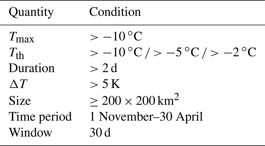
In a first step, a temperature threshold for an initial detection of a potential warm air intrusion is set at ∘C. Especially in the marginal ice zone, the daily 2 m max. air temperature can sometimes fluctuate from day to day around this threshold even if no warm air intrusion (WAI) is present. In order for the WAI to be further considered, the duration during which this temperature threshold is crossed must be at least 2 consecutive days. A minimum ΔT of 5 K between the peak temperature and background temperature is chosen to ensure that a real warm air intrusion is detected and exclude cases were the temperature only fluctuates around a threshold (e.g., in late spring where the average temperatures can easily be above −10 ∘C). Similarly, a minimum size of the detected area of 200 × 200 km2 is required. Table 1 summarizes the set of conditions for the initial detection of a warm air intrusion.
During the detection, a land mask, a polynya mask and a dynamic ice edge mask are applied. The ice edge mask is derived from the minimum extent of SIC >65 % during the 30 d period. By analyzing all warming events, we found that the sea ice concentration in the central Arctic from the OSI SAF algorithm never drops below 65 % in the areas affected by a WAI. Thus, this number is a good compromise in order to include as many warm air intrusions as possible while reducing the effect of a moving ice edge on the results. For the polynya mask, we analyzed 41 years of winter OSI SAF sea ice concentration and masked out areas where the SIC frequently (>15 % of the days) dropped below 50 % while the ice edge was far away. Masked out areas are, e.g., around Svalbard or Novaya Zemlya (see Fig. 2).
The threshold detection interacts with the similarity check procedure. Here, it is tested if the current detected warm air intrusions are similar to the previously detected ones. First, the overlapping area of the new and previous warm air intrusion is calculated. If the overlap is above 70 %, the larger intrusion is used for further calculations, and the other one is discarded. If the extent of both intrusions is similar, the warm air intrusion with the larger effective area reduction (see Sect. 3.2) is used.
In the next step, the detected areas are combined with the sea ice concentration datasets and the effective area reduction procedure is applied. In this module, the effective area reduction (see Sect. 3.2) is calculated for each sea ice concentration dataset and for each defined threshold. The data are finally stored in the output array. In this study, the algorithm is applied for the winter season of November–April. With a 5 d time step, in each iteration, 30 d of 2 m max. air temperature and sea ice concentration are analyzed. A sensitivity test showed that a 5 d step is needed to ensure that the warm air intrusions are optimally captured while the processing time of a season remains reasonably short.
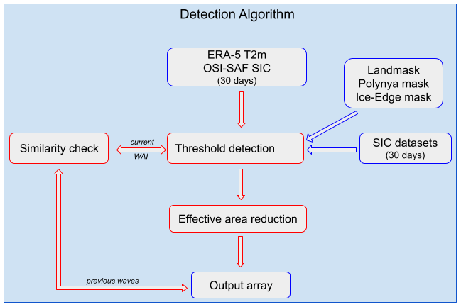
Figure 1Overview of the warm air intrusion detection algorithm. Here WAI is the abbreviation for warm air intrusion.
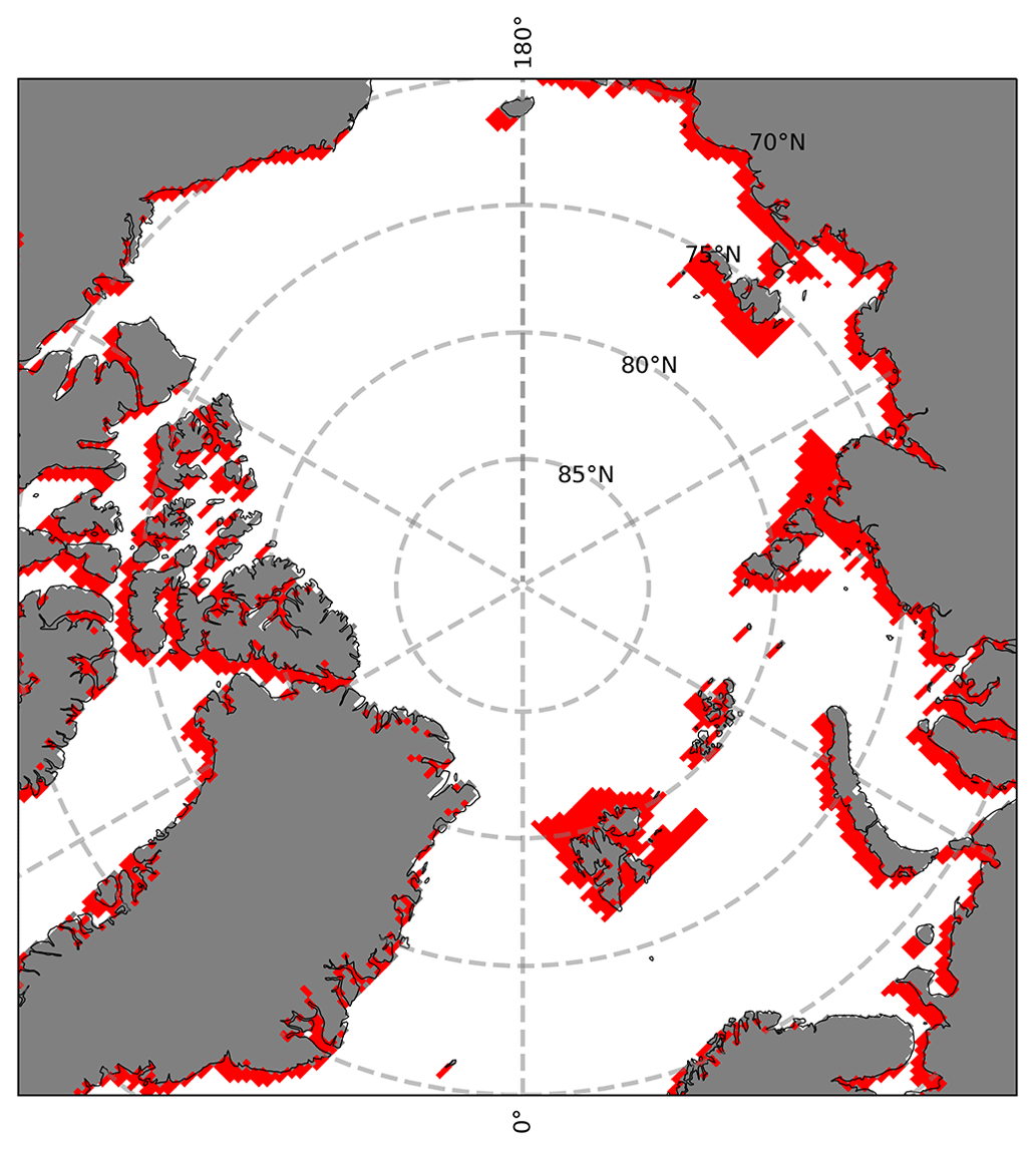
Figure 2Extended landmask used in the algorithm. Gray areas indicate the landmask, and red areas indicate the area where the polynya mask is applied.
Table 1Parameters for the initial warm air intrusions detection. Tmax is the threshold of the temperature maximum that needs to be crossed to trigger the algorithm. Tth is the threshold temperature of the three different warm air intrusion categories. ΔT is the temperature difference between the Tmax and the background temperature (i.e., the average temperature prior and after the warming event). A minimum size of 200 × 200 km2 (of connected warming) is required. Time period describes the period where the algorithm is applied, and window describes the range of days the data are analyzed for.
3.2 Effective area reduction
In order to break the impact of the warm air intrusions on the sea ice concentration to down one number, the effective area reduction is defined. This parameter describes the effective area reduction due to a reduction of sea ice concentration during the period impacted by a warm air intrusion in comparison to the reference sea ice concentration before and after the event. Figure 3 shows the basic principle of this calculation. Shown are the sea ice concentration and the daily max. 2 m air temperature averaged over the area where the threshold ∘C was crossed. The maximum affected area by this warm air intrusion was around 2×10⁶ km2. The average sea ice concentration is above 99 % before and after the event and drops to 95% during the warm air intrusion (red). The resulting effective area reduction, i.e., the sum of the differences between SIC reduced and the average reference SIC, is 6×10⁵ km2 over the whole red period (16 d) or ≈2 % d−1.
Defining the time period during which the sea ice concentration is affected by the warm air intrusion is not straight forward. In this study, the following procedure was chosen: the start of the affected period (SIC reduced) is based on the day when the daily max. 2 m air temperature first crossed the ∘C mark. The end of the period is reached when the sea ice concentration is close (within 1 %) to the reference sea ice concentration. If the latter does not apply, the end of the affected period is set to 10 d after the maximum of the SIC reduction. The value of 10 d was chosen manual by analyzing several detected warm air intrusions. We found that most of the times, after 10 d, the effect of warm air intrusions on the sea ice concentration is negligible. The reference SIC (blue lines) is the average of the sea ice concentration before and after the warming events. In this example, the drop in SIC around day 10 is related to a different WAI and thus excluded in the analysis.
3.3 Sensitivity of choice of detection parameters
We note that the calculated effective area reduction is dependent on the choice of parameters (reference periods, affected period, iteration step length). We performed a sensitivity study, varying the controlling parameters for five test warm air intrusions to estimate their impact on the effective area reduction. In the example given in Fig. 3, varying the start and end dates for the affected period (red line) by ±2 d would lead to changes in effective area reduction of around 5 %. Varying the selection of the reference period in a similar way led to changes of around 3 %. Reducing the iteration step to 1 d instead of 5 d to find the optimal window for the warm air intrusions did not lead to relevant changes for the example shown above. Analyzing five selected large warm air intrusions (March 1990, December 2016, April 2015 and 2020, and February 2020), on average, the effective area reduction varied by ±6 % due to varying the reference periods and affected periods as described above. In two cases, optimizing the warm air intrusion detection by using an iteration step length of 1 d increased the effective area reduction by more than 3 % and 7 %, respectively. For the other cases, no relevant changes were observed. In conclusion, an uncertainty in effective area reduction of roughly 5 % can be expected to be introduced by using fixed parameters for the warm air intrusion detection.
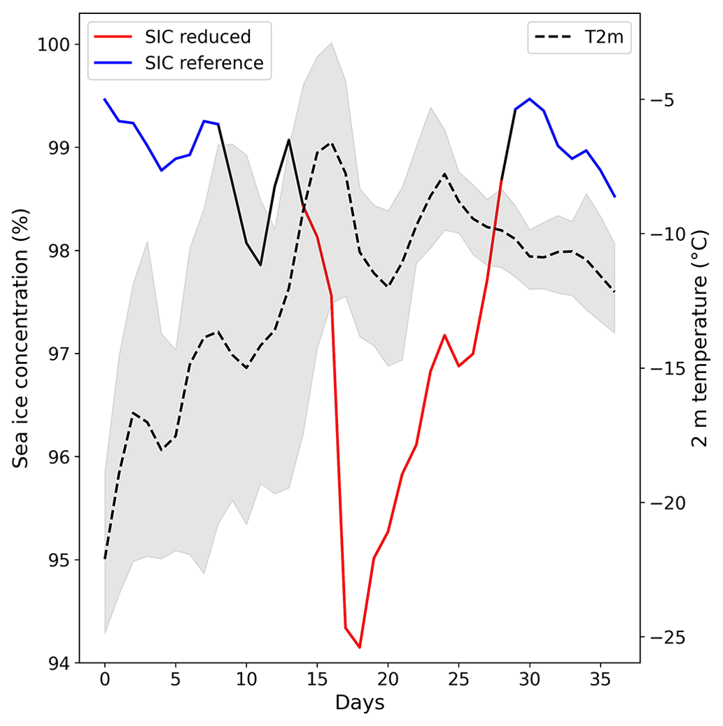
Figure 3Example for the effective area reduction calculation. The sea ice concentration is an average over the whole area affected by the warm air intrusion (around 2×10⁶ km2). Gray shading indicates the 10th and 90th percentiles of the daily max. 2 m air temperature.
4.1 Example of warming events
In this section, two strong warm air intrusions are discussed in detail. These two exceptional warm air intrusions crossed the majority of the sea-ice-covered Arctic in April 2015 and April 2020 (Figs. 4 and 5). For both warm air intrusions, temperatures crossed − 5 ∘C for a large fraction of the area influenced by the warming wave (orange) and − 2 ∘C in some areas (red). Figure 4, top left, shows the maximum extent where the warming peak crossed the different temperature categories. The white color refers to the sea ice cover which is not influenced by the warm air intrusion and blue to the open ocean. In the first row, panels 2 to 5 show the sea ice concentration from four different algorithms, averaged over the whole area affected (all categories, panel 2), the area with −10 ∘C ∘C (panel 3), the area with −5 ∘C ∘C (panel 4), and the area with ∘C (panel 5), respectively. In the second row, the left panel shows the average daily max. air temperature for the whole area influenced by the warm air intrusion (i.e., where the warming crossed −10 ∘C), with gray shading indicating the 10th and 90th percentiles. Rows 2 to 5 show the sea ice concentration retrieved by the different algorithms. The day shown refers to the minimum sea ice concentration in the −5 ∘C ∘C category. This day can be different for the individual algorithms (see individual maps).
At its maximum extent, the warm air intrusion covered the Fram Strait as well as most parts of the central Arctic, overall extending to an area of 337×104 km2. The strongest drop in sea ice concentration by the OSI SAF and NASA-Team algorithms happened in the area where the temperature crossed −2 ∘C. However, the area covered by this category is small. The overall impact on the sea ice area is largest for category 2 for all algorithms. The effective area reduction (i.e., the overall reduction of sea ice area due to sea ice concentration underestimations; see Sect. 3.2) is calculated for the days from 16 to 26 April and is 52×104 km2 for the NASA-Team, 78×104 km2 for the OSI SAF and 112×104 km2 for the ASI algorithm. The overall loss for the NSIDC CDR is small ( km2). For individual days, the effective area reduction can be up to 9×10⁴ km2 for the OSI SAF algorithm and 19×104 km2 for the ASI algorithm. For the first category, i.e., at −10 ∘C, the influence of the warm air intrusion is small for all retrieval algorithms (e.g., km2 for the OSI SAF algorithm).
Figure 5 shows the same as Fig. 4 but for a warm air intrusion reaching the Arctic in April 2020. This warm air intrusion is described in detail in Rückert et al. (2023). The authors attributed the false reduction in sea ice concentration to the formation of a large-scale glaze ice layer, lasting more than a week after the warming event. The real sea ice concentration remained close to 100 % in the central Arctic during and after the warming air intrusion. In the warming category 2, the performance of the different algorithms is similar to the 2015 warm air intrusion discussed before, except for the NASA-Team algorithm, which shows a stronger response compared to the previously discussed warm air intrusion. It is interesting to note that while the sea ice concentration starts recovering for the ASI algorithm towards the end of April, both the NASA-Team and OSI SAF SIC remain reduced, indicating that the effect of the warming event might last longer for these algorithms. In the third category, the drop in sea ice concentration is most pronounced for the OSI SAF and NASA-Team algorithms. Similar to the example from 2015, the overall loss of the NSIDC product is much smaller (40×104 km2) than for the other algorithms: 106×104 km2 for OSI SAF, 120×104 km2 for ASI and 132×104 km2 for the NASA-Team algorithm. In both examples, the day of minimum sea ice concentration is consistent within the products except for the NSIDC algorithm. However, the overall sea ice concentration reduction for the NSIDC CDR is very low, and thus the results are less meaningful for the NSIDC retrieval.
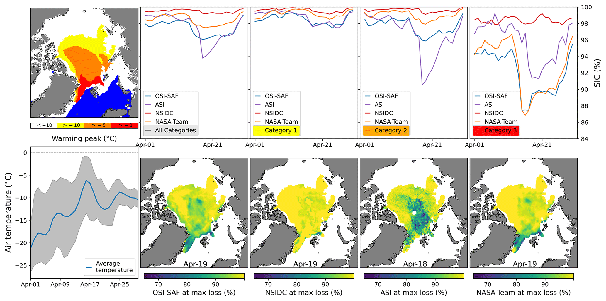
Figure 4April 2015 warm air intrusion and its influence on the four different sea ice concentration products. The top panel shows the extent of the warm air intrusion subdivided into three temperature categories, i.e., −10, −5 and −2 ∘C (left) for the time period between 1 April and 1 May, and the average sea ice concentration for each category. Bottom panel (left) shows the average air temperature for the whole area influenced by the warming event (i.e., daily max. 2 m air temperature ∘C). Gray shading indicates the 10th and 90th percentiles. Columns 2–5 show the sea ice concentration for the different retrievals for the day when their respective ice concentration for the influenced area is lowest (the minimum ice concentration is calculated for the ∘C category). The date is given in the figure.
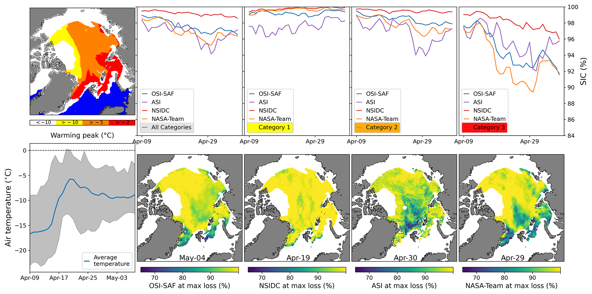
Figure 5April 2020 warming wave and its influence on the three different sea ice concentration algorithms. The top panel shows the extent of the warming wave subdivided into three temperature categories (left) and the average sea ice concentration for each category for the time period between 9 April and 9 May. The bottom panel (left) shows the average air temperature for the whole influenced area (i.e., daily max. 2 m air temperature ∘C). Gray shading indicates the 10th and 90th percentiles. Rows 2–5 show the sea ice concentration for the different retrievals for the day where their respective ice concentration for the influenced area is lowest (the minimum ice concentration is calculated for the ∘C category). The date is given in the figure.
4.2 Statistical results
In this section, we analyze the impact of all warm air intrusions detected during the 41-year period from December 1979 to April 2020. The results are shown in terms of effective area reduction caused by the influence of the warm air intrusions. A full definition of this parameter is given in Sect. 3.2. Here, we want to remind the reader that this effective area reduction is mainly due to too low retrieved sea ice concentration during (and after) the air intrusions. As described in Sect. 3, the best efforts have been made to exclude other effects (ice breakup, polynya opening, melting) that could lead to a natural decrease of sea ice concentration. The influence of potential natural processes that reduce the ice concentration during warm air intrusions are discussed in Sect. 5.3. A full overview of all warm air intrusions detected during the 41-year period is given in Fig. 6, left. Figure 6, right, shows only the largest warming events (65th percentile of the largest effective area reduction) of the OSI SAF algorithm. The individual dots represent the effective area reduction due to the individual warm air intrusions for the three sea ice concentration products (the NASA-Team algorithm is not shown since it performs similarly to the OSI SAF algorithm). The black line shows the number (#) of warm air intrusions detected for one season. While there is only a slight increase in the number of overall events (left), there is an increasing trend (1.17 events per decade) of large events (right) which is, however, not significant (p value >0.05) due to the large inter-annual variability.
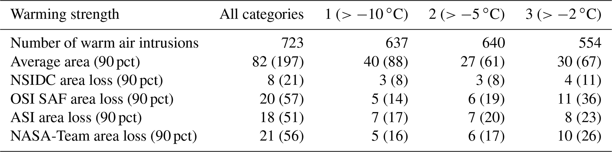
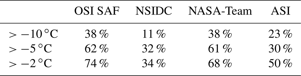
Table 2 summarizes the average area affected by warming events for the three different categories as well as the average effective area reduction of the different sea ice concentration retrievals. All categories refer to all the areas where the temperature crossed − 10 ∘C. It is not necessarily the sum of the individual categories, since the effective area reduction is calculated and optimized for every individual category. In total, 723 warm air intrusions are detected. The number of warm air intrusions of category 1 and 2 are similar; roughly 100 warm air intrusions less were detected in category 3. Overall, the NSIDC CDR product performs best with very little effective area reduction. The other three retrievals show quite similar performance. In category 1 and 2, the ASI algorithm shows a slightly stronger impact, while for category 3, the NASA-Team and OSI SAF algorithms have the strongest response. In the warming detection algorithm, we additionally analyze the areas where the warm air intrusion originates from. Over 70 % of all detected waves originate from the Atlantic sector of the Arctic. Overall, small events, mainly occurring close to the ice edge in the Atlantic sector, are most frequent (not shown here).
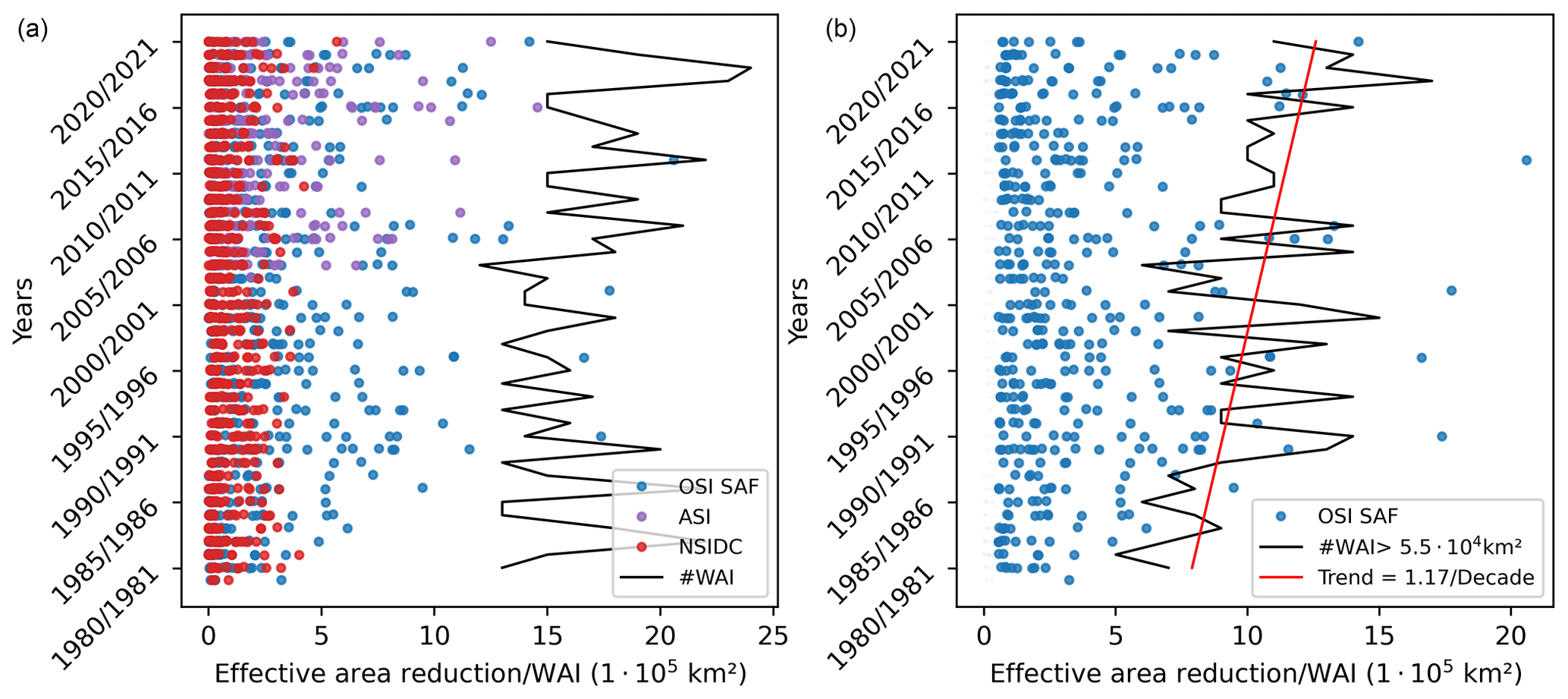
Figure 6(a) Effective area reduction of the three sea ice concentration algorithms for each detected warm air intrusion in the 41-year period from November 1979 to April 2020 (the NASA-Team algorithm is not shown since it performs similar to the OSI SAF algorithm). In addition, the number of warm air intrusions (WAIs) per season is shown as a black line. Panel (b) is the same as (a) but only for large ( km2) warm air intrusions and for the OSI SAF algorithm. In addition, the trend of the number of strong warm air intrusions is given.
Table 2Statistical overview of all detected warm air intrusions. Values of averages are given in 1 × 10⁴ km2. The values in brackets are the 90th percentile of the data.
The performance of the individual sea ice products is compared in Fig. 7. The top left shows a boxplot diagram of the effective area reduction divided by the whole sea ice cover impacted by the warming events (%) for the three categories. For all retrievals, the impact of the warm air intrusions increases with the temperature threshold reached by the warm air intrusion. The NSIDC product is only moderately influenced by the warm air intrusions; only for the third category, the average impact is above 1 %. In this third category, the OSI SAF and NASA-Team algorithms show the strongest impact. Comparing the time periods from 1979–1990 (Fig. 7, bottom left) and 2010–2020 (Fig. 7, bottom right), the average loss is similar for the warm air intrusions of category 1. In categories 2 and 3, an increased effective area reduction is observed in recent years for the OSI SAF and NASA-Team algorithms, supporting the increased trend shown in Fig. 6, right. For example, the mean (median) effective area reduction for the OSI SAF retrieval for category 3 is 3.7 (2.6) for the early period and 4.0 (3.6) for the late period. A similar increase is found for the NASA-Team algorithm.
Figure 7, top right, shows the 41-year average of effective area reduction for the OSI SAF algorithm for the different months from December to April. In April, the warm air intrusions of category 3 clearly have the strongest impact on the performance of the OSI SAF algorithm, with an average monthly effective area reduction of 15.8×10⁴. A similar pattern can be found for the other algorithms (except for NSIDC, see Fig. A1). Splitting the analysis of the monthly effective area reduction to the periods of 1979–1989 and 2010–2020, the effective area reduction in April for category 3 is twice as large in the latter decade (Fig. A2). In other months, the differences are less pronounced.
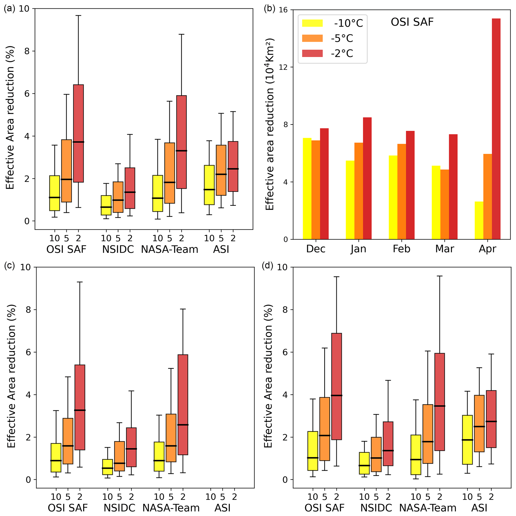
Figure 7(a) Boxplot of the effective area reduction (%) of the four sea ice concentration algorithms and the three different warming classes. The boxes show the 25th and 75th percentiles. In addition, the medians (black line) and 10th and 90th percentiles (whiskers) are given. (b) Monthly distribution of the effective area reduction for the OSI SAF algorithm (average over 41 years). Panels (c) and (d) are the same as panel (a) but for the winters 1979–1990 (c) and 2010–2020 (d). Note that no ASI data are available before 2002.
Figure 8 shows the time series of the effective area reduction during April and December for the OSI SAF, NSIDC and ASI algorithms for warm air intrusions of category 3. The NASA-Team algorithm is not shown here, as it performs very similarly to the OSI SAF algorithm. Note that November, the first month of our analysis, is not shown since during this month the impact of new-forming ice and cracking of ice makes the calculation of the effective area reduction more uncertain. In April, most of the warm air intrusions with a strong impact occur in the last 2 decades, as is visible for the OSI SAF and ASI algorithms. A similar increase of strong warm air intrusions is also found in category 2 (not shown). In December, no increase in effective area reduction, but rather a period with stronger warm air intrusions, between 1983 and 1992 is found. After this period, only in a few individual years (e.g., 2003 and 2007), strong category 3 waves are detected. No increase of warm air intrusions of category 2 or 3 could be found in other months (not shown). We, however, note that in January (February) almost no strong warm air intrusions of category 3 were detected before 1990 (1986) (not shown).
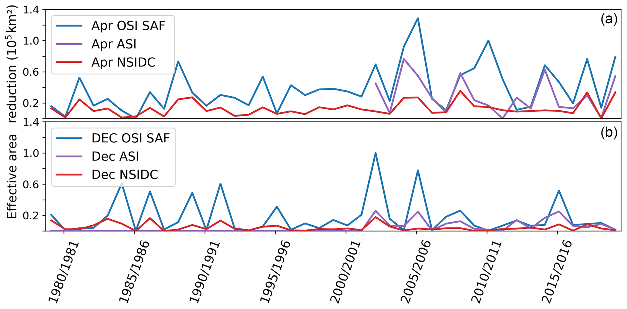
Figure 8Time series of the effective area reduction for April (a) and December (b) for warm air intrusions of category 3 ( ∘C).
The results presented in Figs. 6 to 8 show that the strength of the warm air intrusions increased in the last 20 years, most pronounced during April. Especially, the impact of warm air intrusions of category 3 strongly increased compared to the earlier years between 1980 and 1990. Not only did the average area of category 3 intrusions increase between the earlier (1980 to 1990 km) and more recent years (2010 to 2020 km) but also the average length of these waves increased from 6 to 8 d (not shown).
5.1 Uncertainty of the warm air intrusion detection method
An accurate uncertainty estimation of the results provided in the previous section is challenging due to the high number of unknowns. A sensitivity test suggest an uncertainty of the method itself of around 5 % (see Sect. 3.3). Additionally, there are several sources of uncertainty which are hard to quantify. In the following, we will give an overview of the uncertainty sources and provide a qualitative estimate of their impact if possible.
ERA5 2 m air temperature has a known a positive bias over Arctic sea ice (Batrak and Müller, 2019; Herrmannsdörfer et al., 2023; Wang et al., 2019). Because of this bias, some warm air intrusions might be wrongly captured by the algorithm. Also, misclassification could be a result of the temperature bias (e.g., an area which is classified as ∘C might belong to the ∘C class in reality).
Especially during November, sea ice can also rapidly grow during a warm air intrusion. Consequently, defining the reference period for the effective area reduction calculation (see Sect. 3.2) can be challenging and is sometimes not possible. Therefore, the results presented here are limited to December–April, even though warm air intrusions frequently occur also during November. In April, after a warm air intrusion, the air temperature can remain high until the end of the winter season (the detection stops at 30 April, but an additional 10 d in May are analyzed to properly define warming events occurring in the last third of April). Consequently, it is sometimes difficult to define the end of a warm air intrusion and to detect a proper reference period. These initially detected warm air intrusions were discarded in the results presented here, and thus the effective area reduction in April might be underestimated.
Strong synoptic events like warm air intrusions can push and/or move the sea ice edge and, due to increased ice dynamics, can lead to the opening and closing of leads. Leads modify the sea ice concentration derived by passive microwave algorithms and thus can influence the calculated effective area reduction. To mitigate this influence, the algorithm is only applied in areas where the sea ice concentration remains above 65 % for the whole period of investigation. This is a conservative approach to ensure that there is no false detection of sea ice reduction due to the warm air intrusion, but consequently the effective area reduction considering the whole sea-ice-covered Arctic can be expected to be higher than presented here.
5.2 Uncertainty estimates of satellite sea ice concentration retrievals
Both CDR algorithms provide an uncertainty estimation. For the OSI SAF algorithm, the uncertainty in the central Arctic (i.e., high sea ice concentration) is usually around 2 %–3 %. In areas with high ice dynamics (high temporal variability in ice concentration), the uncertainty can increase to 5 %. A similar increase in uncertainty is also visible under the effect of strong warm air intrusions (e.g., category ∘C or higher). During strong warm air intrusions, sea ice concentration can drop by more than 10 % for a substantial amount of grid cells, meaning that this drop in SIC is not fully covered by an increase of uncertainty.
For example, for the two warming events discussed in detail in the results section (Figs. 4 and 5), 60 % (Fig. 4) and 35 % (Fig. 5) of the area affected ( ∘C, reference SIC > 95 %), the reduction of sea ice concentration was larger than the uncertainty estimate of the OSI SAF algorithm (at the maximum sea ice concentration reduction). Similar results were found for warm air intrusions ∘C in the high sea ice concentration domain. It is important to note that large parts of the ∘C warm air intrusions happen in the marginal ice zone in the intermediate sea ice cover domain (50 % < SIC < 75 %); here, the uncertainty of the OSI SAF algorithm is higher and often as high as the reduction in SIC due to the warm air intrusions.
The NSIDC CDR provides a quality assessment and a standard deviation to estimate the uncertainty of the sea ice concentration. The standard deviation of a grid cell is estimated from the nine surrounding grid cells from each sub-algorithm used (NASA-Team and Bootstrap). In the central Arctic it is usually between 0 % and 2 %, but it can be 10 % and higher in the marginal ice zone. As shown in Fig. 7, the NSIDC CDR is overall less influenced by warm air intrusions, and mainly the ∘C warm air intrusions have an impact on the derived ice concentration. For warm air intrusions ∘C in the high sea ice concentration domain, we find that in 25 %–40 % of the cases the sea ice reduction is higher than the uncertainty of the retrieval. It is important to note that the sea ice concentration reduction of individual grid cells is rarely above 5 % in the NSIDC CDR. Overall, the effect of the warm air intrusions is not fully captured by the uncertainty of both CDR algorithms. An increased uncertainty needs to be considered in the case of strong warming events.
Since the NSIDC CDR is way less influenced by warm air intrusions, it is worth discussing the reason for its good performance in our study. The NSIDC CDR is computed from the NASA-Team (Cavalieri et al., 1997) and Bootstrap (Comiso, 1986) algorithms. The CDR sea ice concentration is based on the sub-algorithm with the higher sea ice concentration, which, in the case of strong warm air intrusions, is usually the Bootstrap algorithm (since the NASA-Team algorithm shows a strong underestimation of sea ice concentration during warm air intrusions). In the NSIDC CDR, an updated Bootstrap algorithm with dynamic (daily adapted) tie points for open ocean and full sea ice cover is used (Comiso et al., 2017). By using dynamic tie points, the impacts of changing snow and surface conditions are mitigated, and thus the impact of warm air intrusions on the derived sea ice concentration is reduced.
While the NSIDC CDR generally performs best during warming events, we note that an overestimation of sea ice concentration can be a result of the method applied in this algorithm. This can especially occur in areas with frequent polynyas and large lead openings after strong storm events, like for example the Greenland Sea. Such real reductions in sea ice concentration are often not captured by the NSIDC CDR, while in the OSI SAF CDR or the ASI algorithm using its natural resolution (6.25 km2), these events are clearly visible (see Fig. 9). Kern et al. (2019) performed an inter-comparison of several sea ice concentration products and found that the NSIDC CDR systematically overestimates sea ice concentration by around 3 % when the ice concentration is close to 100 %. This overestimation is not visible in the final product, since the NSIDC CDR is truncated at 100 % ice concentration. Therefore, in the case of strong warm air intrusions, the NSIDC CDR sea ice concentration can remain close to 100 % even though the (non-truncated) ice concentration would drop by a few percent (e.g., from 103 % to 99 %).
The results of this study show that, in recent years, high impact warm air intrusions have become more frequent, and their impact on satellite sea ice algorithms became stronger (Fig. 8). With further Arctic warming, it is likely that strong warm air intrusions will occur even more frequently and might extend to earlier months in the year, although no such trend was observed for, e.g., March in this study. The associated increased uncertainty in winter time satellite-derived sea ice concentration needs to be addressed. In principle, a warm air intrusion detection algorithm as presented here could be used to reprocess sea ice climatologies, “correcting” for the impact of strong warm air intrusions. However, currently the high uncertainty of this method due to, e.g., not considering leads, flagging out the marginal ice zone area or the choice of the reference sea ice concentration period make it difficult to reliably correct sea ice concentrations. Further improvements of this approach and additional datasets (e.g., synthetic aperture radar lead classification) are needed. A more simple approach could aim for including air temperature variability in the uncertainty estimation. This could help to improve the winter time uncertainty estimation, especially in the central Arctic, where strong warm air intrusions are one of the main sources for uncertainty.
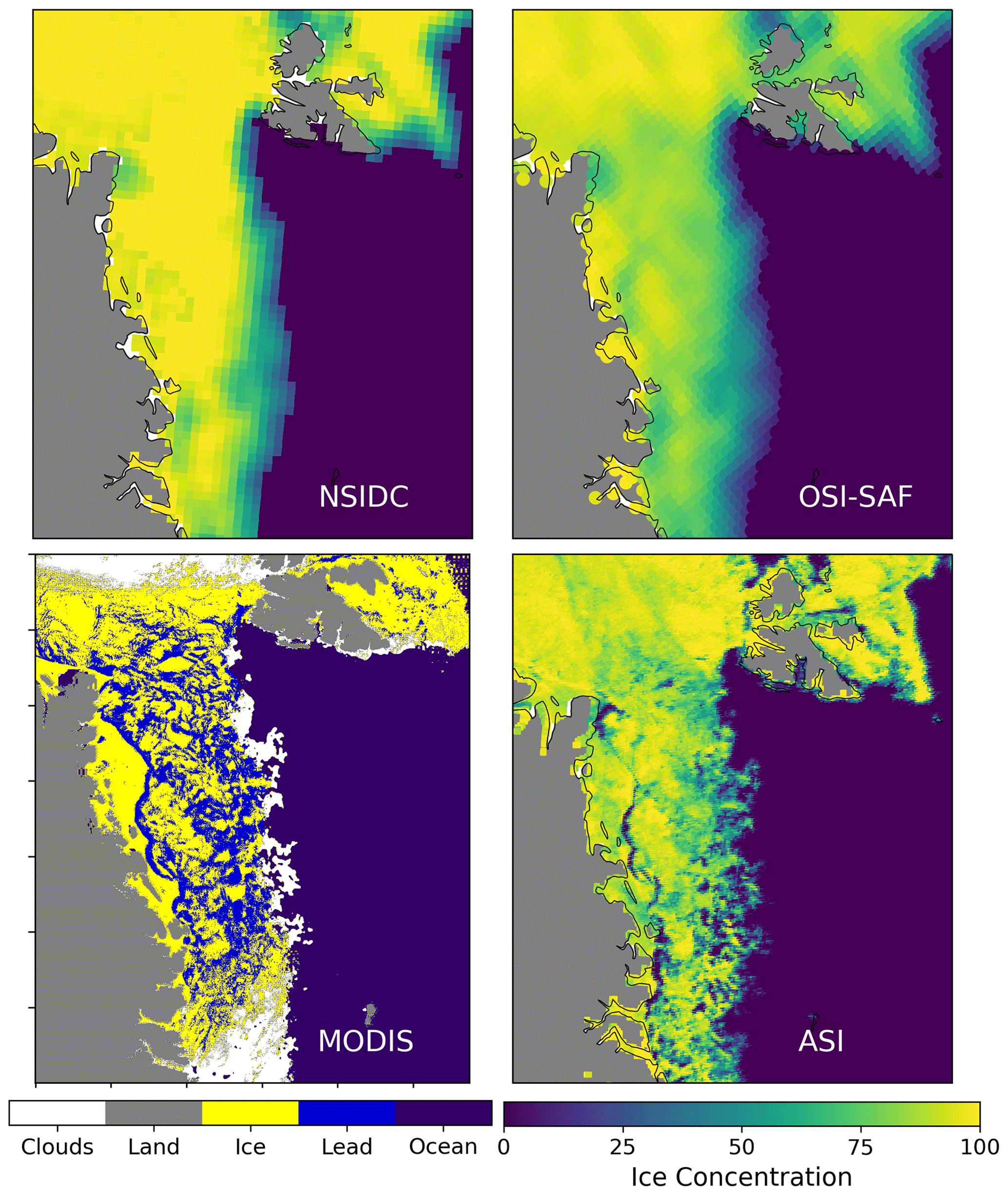
Figure 9Sea ice concentration in the Fram Strait for 20 April 2020 for three different algorithms. In addition, sea ice leads derived from MODIS (Willmes and Heinemann, 2015) are shown.
5.3 Sea ice concentration reduction
Aue et al. (2022) analyzed the impact of cyclones on the sea ice concentration in the Atlantic sector of the Arctic ocean and found an average drop in sea ice concentration of less than 2 % in ±3 d around the cyclone events. The drop in SIC was stronger close to the ice edge and in the low ice concentration regimes. Almost no drop in sea ice concentration was found in the central Arctic.
Table 3 shows the cases detected of warm air intrusions (%), during which the average sea ice concentration reduction is above 2 % for the three different categories. For warm air intrusions of category 2 or 3, the majority of warm air intrusions (>60 %) led to a reduction of SIC >2 % for the OSI SAF and NASA-Team algorithms. In comparison, for the NSIDC and ASI algorithms only about 30 % of the warm air intrusions in category 2 caused a reduction of >2 %. For category 3, almost 50 % of all warming events caused a sea ice concentration reduction of >2 % for the ASI algorithm which, however, is still well below what was found for OSI SAF and NASA-Team (roughly 70 %). It is important to keep in mind that, in this study, SIC reduction was averaged over the whole affected period, which is much longer (up to 12 d) than the 6 d considered in the study by Aue et al. (2022). More than 5 d after the cyclone event, Aue et al. (2022) reported a SIC increase in most of the areas in the Arctic and only an average reduction of <1 % in the Greenland Sea. Using a threshold of 1 % SIC reduction in our analysis, for OSI SAF, NASA-Team and ASI, over 80 % of the warm air intrusions (for category 2 and 3) caused an average sea ice concentration reduction above the 1 % threshold. Only the NSIDC algorithm remains below this threshold in roughly 50 % of the cases. Another recent study found similar effects of cyclones on the sea ice concentration (Clancy et al., 2021), leading to a reduction in ice concentration between 1 %–3 %, with the strongest effects in the marginal ice zone. Graham et al. (2017) found a strong storm-introduced reduction of sea ice concentration in February 2015 north of Svalbard during the N-ICE2015 drift campaign. A detailed analysis showed that for the February 2015 warm air intrusion (as detected with the here-presented algorithm), the area around (and south of) the campaign location was masked out since the automatic ice edge and polynya masks triggered (see Sect. 3). The remaining effected area was of medium size (5×10⁵ km2), and the sea ice reduction (e.g., 2.5 % for the OSI SAF algorithm) was not exceptional. The Aue et al. (2022), Clancy et al. (2021) and Graham et al. (2019b) studies attribute the changes in SIC to natural causes implied by the passing cyclone and not to a deficiency of the satellite SIC products.
These findings demonstrate that in the majority of the warm air intrusions or cyclones, one can expect a natural and real change in SIC of 1 %–3 %, e.g., by opening of leads. The reduction in sea ice concentration that we find for warming events (for some algorithms >2 % SIC reduction in >60 % of the cases, see Table 3) is thus more than what would be expected due to potential increased lead openings. This is especially true for the strong warm air intrusions, where we often found the impact of the warming event on SIC to last up to a week after the event. In summary, we find that during and after warm air intrusions, the reduction of sea ice concentration by all algorithms (except for the NSIDC CDR) is, in many cases, higher than what would be expected by the opening of leads due to sea ice dynamics.
Table 3Cases of warm air intrusions during which the average sea ice concentration dropped by more than 2 % for the three different temperature thresholds.
In this study, we analyzed the impact of warm air intrusions on sea ice concentration climatologies derived from microwave radiometer satellite measurements. We investigated the following questions: (I) is the impact of warm air intrusions on satellite-based sea ice concentration algorithms a relevant source of uncertainty for sea ice climatologies? (II) Did the recent amplified temperature increase in the Arctic lead to an increase in frequency and extent of winter warm air intrusions? Has the impact of warm air intrusions on satellite sea ice concentration algorithms increased in recent years?
- I.
Based on the results presented here (e.g., Figs. 4, 5 and 7), we have shown that warm air intrusions can have a strong impact on most sea ice concentration algorithms (except the NSIDC CDR), leading to an underestimation of sea ice concentration and consequently an underestimation of sea ice area. Depending on the algorithm, this underestimation is on average between 2 % and 4 % of the total area affected by the warm air intrusion (Fig. 7) for warm air intrusions of category 3. For large warm air intrusions (e.g., in April 2015, Fig. 4), the effective sea ice area reduction is in the order of 78×104 to 115×104 km2 (OSI SAF and ASI) over the whole influenced period (9 d) and up to 19×104 km2 for a single day (ASI). During strong warm air intrusions, reduction in sea ice concentration due to the warming is often not fully captured in the uncertainty of both CDR products.
- II.
In general, we found that warm air intrusions of category 3 (i.e., the warmest >2 ∘C category) are most prominent in April (Fig. 7, top right) and that in April they have an increased impact on the satellite algorithms in the last 2 decades (Fig. 8). For the other months, no such increase is evident in the data. In the scope of further climate change, it can be expected that such warm air intrusions will become even more frequent and that category 3 intrusions will extend further into the central Arctic. During strong warming events the NSIDC CDR benefits from including the Bootstrap algorithm (Comiso, 1986), which is less sensitive to the impact of the warm air intrusions on the snow-covered sea ice system. In general, lower frequencies (e.g., 6.9 GHz) are less influenced by warm air intrusions (Rückert et al., 2023), since these are mainly short-term events, and the warming rarely reaches the snow–ice interface where the low-frequency signal mainly originates. With future higher-resolution low-frequency observations (e.g., the CIMR – Copernicus Imaging Microwave Radiometer), such algorithms using lower frequencies could be used as a reference for correcting current algorithms during strong warm air intrusions.
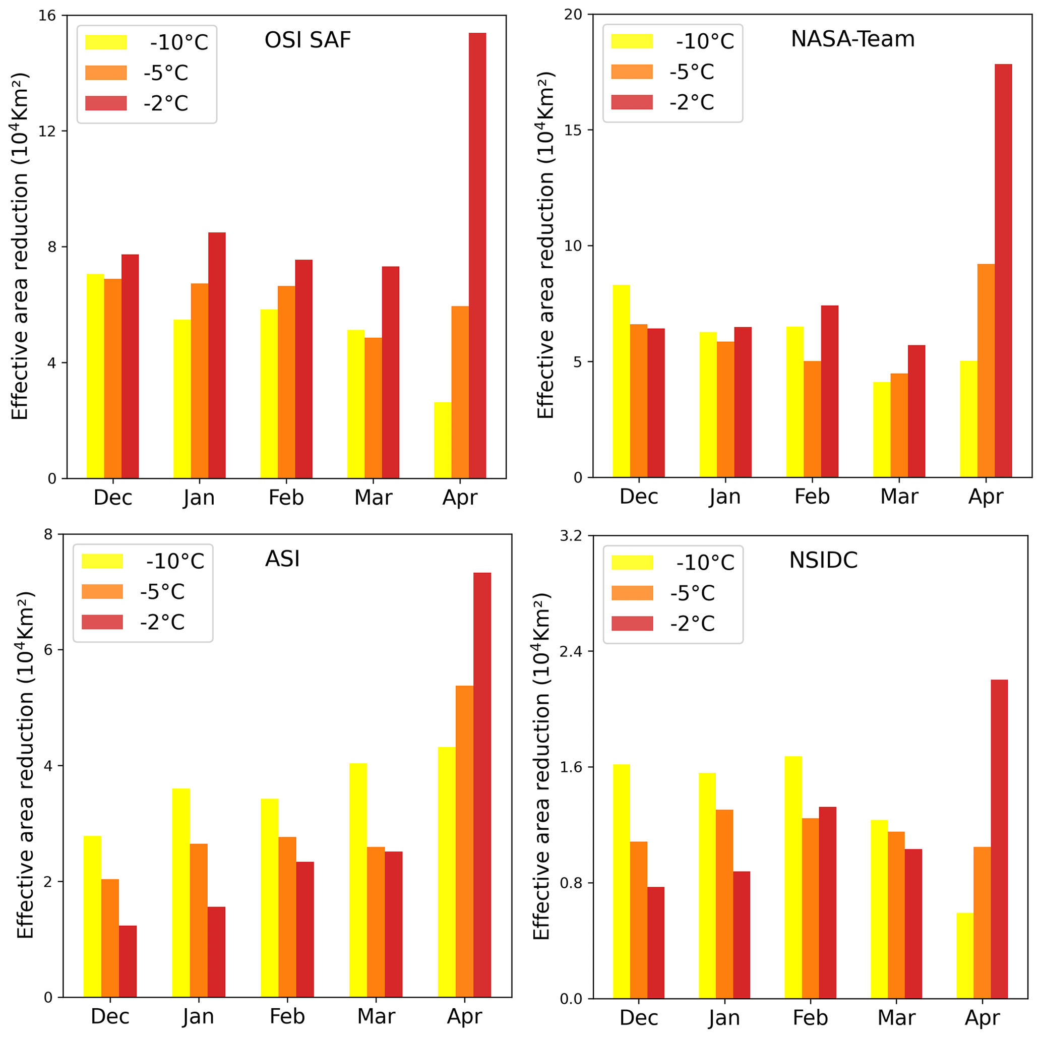
Figure A1Monthly distribution of the effective area reduction for the four different algorithms (averaged over 41 years). Note that the scale of the y axis is different for each panel.
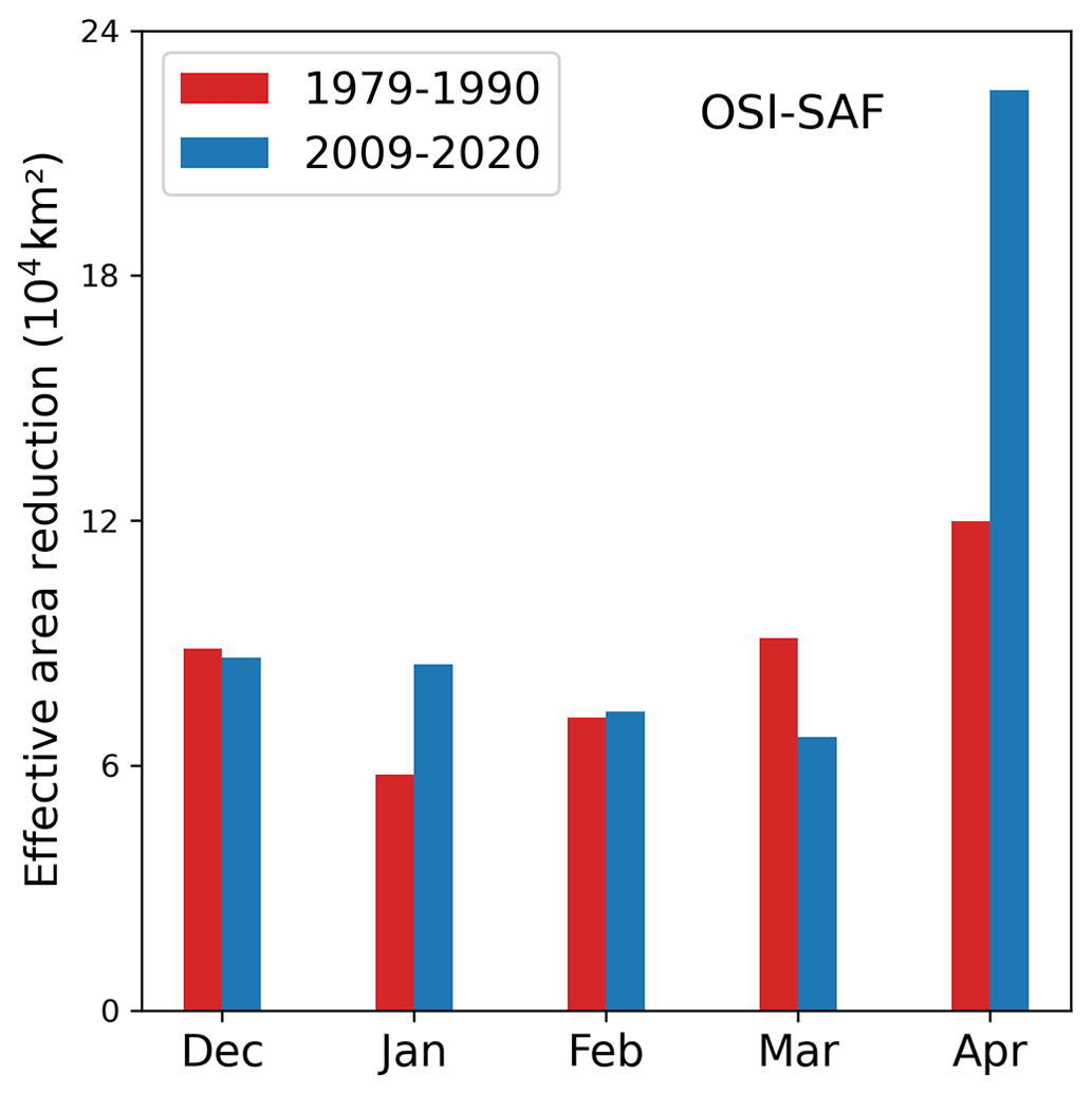
Figure A2Monthly distribution of the effective area reduction for the OSI SAF algorithm for the years 1979–1990 and 2009–2020 and for warm air intrusions of category 3 (i.e., daily max. 2 m temperature ∘C).
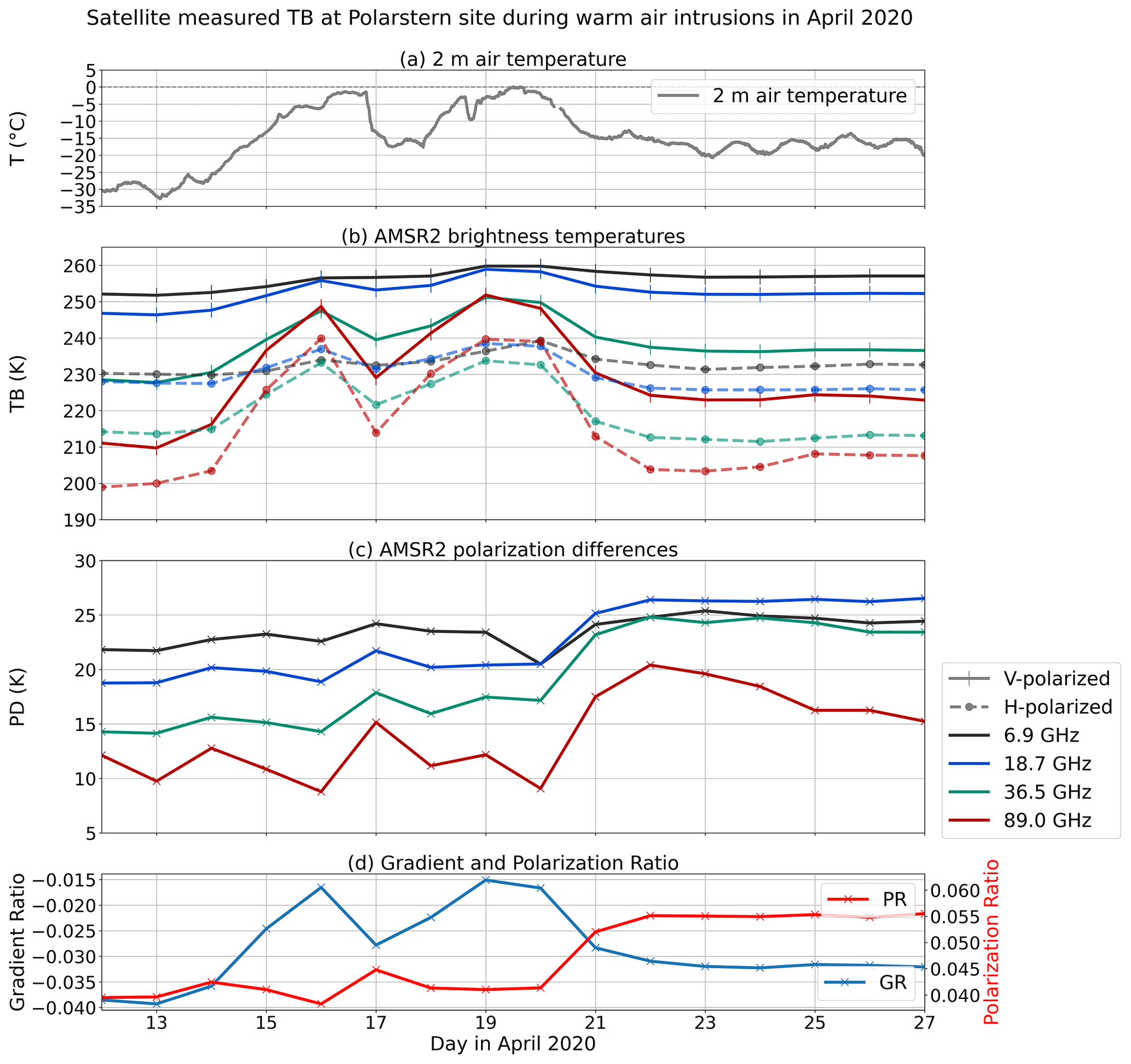
Figure A3Figure 4 from Rückert et al. (2023): panel (a) shows the daily max. air temperature at 2 m. Collocated satellite measurement of brightness temperature (TB) (b) and polarization difference (PD) (c) around Polarstern (daily averages). (d) Gradient ratio of 36.5 and 18.7 GHz and polarization ratio of 18.7 GHz.
The NSIDC CDR and NASA-Team sea ice concentrations used in this study are available via https://doi.org/10.7265/efmz-2t65 (Meier et al., 2021). The OSI SAF CDR is available via https://osi-saf.eumetsat.int/products/osi-450-a (OSI, 2023), and the ASI ice concentration can be downloaded from https://data.seaice.uni-bremen.de/amsr2/asi_daygrid_swath/n6250/ (last access: 4 September 2023; Spreen et al., 2008). The ERA5 2 m air temperature data can be obtained from https://cds.climate.copernicus.eu/cdsapp#!/home (last access: 3 November 2023). The core algorithm and an overview file of all detected warm air intrusions is available at https://doi.org/10.5281/Zenodo.8160071 (Rostosky, 2023).
PR performed the study and wrote the initial version of the article. GS contributed to the discussion and development of the study. All authors revised and commented on the article.
The contact author has declared that neither of the authors has any competing interests.
Publisher’s note: Copernicus Publications remains neutral with regard to jurisdictional claims in published maps and institutional affiliations.
This work was funded by the Bundesministerium für Bildung und Forschung (BMBF) through the IceSense project (grant no. BMBF 03F0866B). Further support was provided by the European Union's Horizon 2020 research and innovation programme (grant no. 101003826) via project CRiceS (Climate Relevant interactions and feedbacks: the key role of sea ice and Snow in the polar and global climate system). We further acknowledge NOAA/NSIDC, Eumetsat OSI SAF and the Copernicus Climate Change Service for providing the sea ice concentration and air temperature datasets used in this study. Further, we thank Sascha Willmes for providing daily sea ice lead data for the Arctic.
This research has been supported by the Bundesministerium für Bildung und Forschung (grant no. 03F0866B) and Horizon 2020 (grant no. 101003826).
The article processing charges for this open-access publication were covered by the University of Bremen.
This paper was edited by Vishnu Nandan and reviewed by two anonymous referees.
Aue, L., Vihma, T., Uotila, P., and Rinke, A.: New Insights Into Cyclone Impacts on Sea Ice in the Atlantic Sector of the Arctic Ocean in Winter, Geophys. Res. Lett., 49, e2022GL100051, https://doi.org/10.1029/2022GL100051, 2022. a, b, c, d, e
Batrak, Y. and Müller, M.: On the warm bias in atmospheric reanalyses induced by the missing snow over Arctic sea-ice., Nat Commun, 10, 4170, https://doi.org/10.1038/s41467-019-11975-3, 2019. a, b
Cavalieri, D. J., Parkinson, C. L., Gloersen, P., and Zwally, H. J.: Arctic and Antarctic Sea Ice Concentrations from Multichannel Passive-Microwave Satellite Data Sets: October 1978–September 1995 User's Guide, Tech. Rep. NASA-TM-104647, NASA Goddard Space Flight Center, https://ntrs.nasa.gov/citations/19980076134 (last access: 20 March 2023), 1997. a, b, c, d
Clancy, R., Bitz, C. M., Blanchard-Wrigglesworth, E., McGraw, M. C., and Cavallo, S. M.: A cyclone-centered perspective on the drivers of asymmetric patterns in the atmosphere and sea ice during Arctic cyclones, J. Climate, 35, 1–47, https://doi.org/10.1175/JCLI-D-21-0093.1, 2021. a, b, c
Comiso, J. C.: Characteristics of Arctic winter sea ice from satellite multispectral microwave observations, J. Geophys. Res.-Oceans, 91, 975–994, https://doi.org/10.1029/JC091iC01p00975, 1986. a, b, c
Comiso, J. C., Cavalieri, D. J., Parkinson, C. L., and Gloersen, P.: Passive microwave algorithms for sea ice concentration: A comparison of two techniques, Remote Sens. Environ., 60, 357–384, https://doi.org/10.1016/S0034-4257(96)00220-9, 1997. a, b
Comiso, J. C., Gersten, R. A., Stock, L. V., Turner, J., Perez, G. J., and Cho, K.: Positive Trend in the Antarctic Sea Ice Cover and Associated Changes in Surface Temperature, J. Climate, 30, 2251–2267, https://doi.org/10.1175/JCLI-D-16-0408.1, 2017. a, b
Drinkwater, M., Hosseinmostafa, R., and Gogineni, P.: C-Band Backscatter Measurements of Winter Sea-Ice in the Weddell Sea, Antarctica, Int. J. Remote Sens., 16, 3365–3389, https://doi.org/10.1080/01431169508954635, 1995. a
EUMETSAT Ocean and Sea Ice Satellite Application: Global sea ice concentration climate data record 1978–2020 (v3.0, 2022), OSI-450-a, https://doi.org/10.15770/EUM_SAF_OSI_0013 [data set], data (for 1979–2020, https://osi-saf.eumetsat.int/products/osi-450-a (last access: 3 July 2023), 2023. a, b
Graham, R. M., Cohen, L., Petty, A. A., Boisvert, L. N., Rinke, A., Hudson, S. R., Nicolaus, M., and Granskog, M. A.: Increasing frequency and duration of Arctic winter warming events, Geophys. Res. Lett., 44, 6974–6983, https://doi.org/10.1002/2017GL073395, 2017. a, b
Graham, R. M., Itkin, P., Meyer, A., Sundfjord, A., Spreen, G., Smedsrun, L. H., Liston, G. E., Cheng, B., Cohen, L., Divine, D., Fer, I., Fransson, A., Gerland, S., Haapala, J., Hudson, S. R., Johansson, A. M., King, J., Merkouriadi, I., Peterson, A. K., Provost, C., Randelhoo, A., Rinke, A., Rösel, A., Sennecheal, N., Walden, V. P., Duarte, P., Assmy, P., Steen, H., and Granskog, M. A.: Winter storms accelerate the demise of sea ice in the Atlantic sector of the Arctic Ocean, Sci. Rep., 9, 9222, https://doi.org/10.1038/s41598-019-45574-5, 2019. a, b
Herrmannsdörfer, L., Müller, M., Shupe, M. D., and Rostosky, P.: Surface temperature comparison of the Arctic winter MOSAiC observations, ERA5 reanalysis, and MODIS satellite retrieval, Elementa: Science of the Anthropocene, 11, 00085, https://doi.org/10.1525/elementa.2022.00085, 2023. a, b
Hersbach, H., Bell, B., Berrisford, P., Hirahara, S., Horányi, A., Muñoz-Sabater, J., Nicolas, J., Peubey, C., Radu, R., Schepers, D., Simmons, A., Soci, C., Abdalla, S., Abellan, X., Balsamo, G., Bechtold, P., Biavati, G., Bidlot, J., Bonavita, M., Chiara, G. D., Dahlgren, P., Dee, D., Diamantakis, M., Dragani, R., Flemming, J., Forbes, R., Fuentes, M., Geer, A., Haimberger, L., Healy, S., Hogan, R. J., Hólm, E., Janisková, M., Keeley, S., Laloyaux, P., Lopez, P., Lupu, C., Radnoti, G., Rosnay, P. d., Rozum, I., Vamborg, F., Villaume, S., and Thépaut, J.-N.: The ERA5 global reanalysis, Q. J. Roy. Meteor. Soc., 146, 1999–2049, https://doi.org/10.1002/qj.3803, 2020. a, b
Ivanova, N., Pedersen, L. T., Tonboe, R. T., Kern, S., Heygster, G., Lavergne, T., Sørensen, A., Saldo, R., Dybkjær, G., Brucker, L., and Shokr, M.: Inter-comparison and evaluation of sea ice algorithms: towards further identification of challenges and optimal approach using passive microwave observations, The Cryosphere, 9, 1797–1817, https://doi.org/10.5194/tc-9-1797-2015, 2015. a
Kern, S., Lavergne, T., Notz, D., Pedersen, L. T., Tonboe, R. T., Saldo, R., and Sørensen, A. M.: Satellite passive microwave sea-ice concentration data set intercomparison: closed ice and ship-based observations, The Cryosphere, 13, 3261–3307, https://doi.org/10.5194/tc-13-3261-2019, 2019. a, b
Kern, S., Lavergne, T., Notz, D., Pedersen, L. T., and Tonboe, R.: Satellite passive microwave sea-ice concentration data set inter-comparison for Arctic summer conditions, The Cryosphere, 14, 2469–2493, https://doi.org/10.5194/tc-14-2469-2020, 2020. a, b
Kern, S., Lavergne, T., Pedersen, L. T., Tonboe, R. T., Bell, L., Meyer, M., and Zeigermann, L.: Satellite passive microwave sea-ice concentration data set intercomparison using Landsat data, The Cryosphere, 16, 349–378, https://doi.org/10.5194/tc-16-349-2022, 2022. a
Kumar, A., Perlwitz, J., Eischeid, J., Quan, X., Xu, T., Zhang, T., Hoerling, M., Jha, B., and Wang, W.: Contribution of sea ice loss to Arctic amplification, Geophys. Res. Lett., 37, L21701, https://doi.org/10.1029/2010GL045022, 2010. a
Lavergne, T., Tonboe, R., Lavelle, J., and Eastwood, S.: Algorithm Theoretical Basis Document for the OSI SAF Global Sea Ice Concentration Climate Data Record, EUMETSAT Ocean and Sea Ice Satellite Application Facility, version 1.1, https://osisaf-hl.met.no/sites/osisaf-hl/files/baseline_document/osisaf_cdop3_ss2_atbd_sea-ice-conc-climate-data-record_v1p2.pdf (last access: 4 September 2023), 2016. a, b, c, d
Lavergne, T., Sørensen, A. M., Kern, S., Tonboe, R., Notz, D., Aaboe, S., Bell, L., Dybkjær, G., Eastwood, S., Gabarro, C., Heygster, G., Killie, M. A., Brandt Kreiner, M., Lavelle, J., Saldo, R., Sandven, S., and Pedersen, L. T.: Version 2 of the EUMETSAT OSI SAF and ESA CCI sea-ice concentration climate data records, The Cryosphere, 13, 49–78, https://doi.org/10.5194/tc-13-49-2019, 2019. a, b, c, d
Liu, G. and Curry, J. A.: Observation and interpretation of microwave cloud signatures over the Arctic ocean during winter, J. Appl. Meteorol., 42, 51–64, https://doi.org/10.1175/1520-0450(2003)042<0051:OAIOMC>2.0.CO;2, 2003. a, b
Maslanik, J., Stroeve, J., Fowler, C., and Emery, W.: Distribution and trends in Arctic sea ice age through spring 2011, Geophys. Res. Lett., 38, L13502, https://doi.org/10.1029/2011GL047735, 2011. a
Meier, W. N., Fetterer, F., Windnagel, A. K., and Stewart, S.: NOAA/NSIDC Climate Data Record of Passive Microwave Sea Ice Concentration, Version 4., Boulder, Colorado, USA, NSIDC: National Snow and Ice Data Center [data set], https://doi.org/10.7265/efmz-2t65, 2021. a, b, c, d, e
Mätzler, C., Ramseier, R., and Svendsen, E.: Polarization effects in seaice signatures, IEEE J. Oceanic. Eng., 9, 333–338, https://doi.org/10.1109/JOE.1984.1145646, 1984. a
Perovich, D. K., Meier, W. Tschudi, M., Farrell, S. L., Hendricks, S., Gerland, S., Haas, C., Krumpen, T., Polashensky, C., Ricker, R., and Webster, M.: Sea ice, Arctic report card 2017, National Oceanic and Atmospheric Administration (NOAA), 2017. a
Rostosky, P.: Wintertime Arctic warm air intrusion detection algorithm for satellite sea ice concentration analysis, Zenodo [data set], https://doi.org/10.5281/zenodo.8160071, 2023. a
Rückert, J. E., Rostosky, P., Huntemann, M., Clemens-Sewall, D., Ebell, K., Kaleschke, L., Lemmetyinen, J., Macfarlane, A., Naderpour, R., Stroeve, J., Walbröl, A., and Spreen, G.: Sea ice concentration satellite retrievals influenced by surface changes due to warm air intrusions: A case study from the MOSAiC expedition, EarthArXiv [preprint], https://doi.org/10.31223/X5VW85, 2023. a, b, c, d, e, f, g, h
Spreen, G., Kaleschke, L., and Heygster, G.: Sea ice remote sensing using AMSR-E 89-GHz channels, J. Geophys. Res., 113, C02S03, https://doi.org/10.1029/2005JC003384, 2008. a, b, c, d, e, f
Stroeve, J., Nandan, V., Willatt, R., Dadic, R., Rostosky, P., Gallagher, M., Mallett, R., Barrett, A., Hendricks, S., Tonboe, R., McCrystall, M., Serreze, M., Thielke, L., Spreen, G., Newman, T., Yackel, J., Ricker, R., Tsamados, M., Macfarlane, A., Hannula, H.-R., and Schneebeli, M.: Rain on snow (ROS) understudied in sea ice remote sensing: a multi-sensor analysis of ROS during MOSAiC (Multidisciplinary drifting Observatory for the Study of Arctic Climate), The Cryosphere, 16, 4223–4250, https://doi.org/10.5194/tc-16-4223-2022, 2022. a
Tonboe, R. T., Andersen, S., and Toudal, L.: Anomalous winter sea ice backscatter and brightness temperatures, Tech. rep., Danish Meteorological Institute, Copenhagen, Sci. Rep., 03-13, https://doi.org/10.13140/RG.2.1.3551.0805, 2003. a, b, c, d
Wang, C., Graham, R. M., Wang, K., Gerland, S., and Granskog, M. A.: Comparison of ERA5 and ERA-Interim near-surface air temperature, snowfall and precipitation over Arctic sea ice: effects on sea ice thermodynamics and evolution, The Cryosphere, 13, 1661–1679, https://doi.org/10.5194/tc-13-1661-2019, 2019. a, b
Willmes, S. and Heinemann, G.: Pan-Arctic lead detection from MODIS thermal infrared imagery, Ann. Glaciol., 56, 29–37, https://doi.org/10.3189/2015AoG69A615, 2015. a