the Creative Commons Attribution 4.0 License.
the Creative Commons Attribution 4.0 License.
 | 06 Sep 2023
Evaluating the impact of enhanced horizontal resolution over the Antarctic domain using a variable-resolution Earth system model
Rajashree Tri Datta
Adam Herrington
Jan T. M. Lenaerts
David P. Schneider
Luke Trusel
Devon Dunmire
Earth system models are essential tools for understanding the impacts of a warming world, particularly on the contribution of polar ice sheets to sea level change. However, current models lack full coupling of the ice sheets to the ocean and are typically run at a coarse resolution (1∘ grid spacing or coarser). Coarse spatial resolution is particularly a problem over Antarctica, where sub-grid-scale orography is well-known to influence precipitation fields, and glacier models require high-resolution atmospheric inputs. This resolution limitation has been partially addressed by regional climate models (RCMs), which must be forced at their lateral and ocean surface boundaries by (usually coarser) global atmospheric datasets, However, RCMs fail to capture the two-way coupling between the regional domain and the global climate system. Conversely, running high-spatial-resolution models globally is computationally expensive and can produce vast amounts of data.
Alternatively, variable-resolution grids can retain the benefits of high resolution over a specified domain without the computational costs of running at a high resolution globally. Here we evaluate a historical simulation of the Community Earth System Model version 2 (CESM2) implementing the spectral element (SE) numerical dynamical core (VR-CESM2) with an enhanced-horizontal-resolution (0.25∘) grid over the Antarctic Ice Sheet and the surrounding Southern Ocean; the rest of the global domain is on the standard 1∘ grid. We compare it to 1∘ model runs of CESM2 using both the SE dynamical core and the standard finite-volume (FV) dynamical core, both with identical physics and forcing, including prescribed sea surface temperatures (SSTs) and sea ice concentrations from observations. Our evaluation reveals both improvements and degradations in VR-CESM2 performance relative to the 1∘ CESM2. Surface mass balance estimates are slightly higher but within 1 standard deviation of the ensemble mean, except for over the Antarctic Peninsula, which is impacted by better-resolved surface topography. Temperature and wind estimates are improved over both the near surface and aloft, although the overall correction of a cold bias (within the 1∘ CESM2 runs) has resulted in temperatures which are too high over the interior of the ice sheet. The major degradations include the enhancement of surface melt as well as excessive cloud liquid water over the ocean, with resultant impacts on the surface radiation budget. Despite these changes, VR-CESM2 is a valuable tool for the analysis of precipitation and surface mass balance and thus constraining estimates of sea level rise associated with the Antarctic Ice Sheet.
- Article
(15076 KB) - Full-text XML
-
Supplement
(9978 KB) - BibTeX
- EndNote


The Antarctic Ice Sheet (AIS) contains the largest amount of fresh water on Earth and, with the Greenland Ice Sheet, is the greatest potential source of future sea level rise (Pan et al., 2021). Satellite observations have captured net mass loss of the AIS (Shepherd et al., 2019), which since 1993 has accounted for approximately 10 % of observed global mean sea level rise (IPCC, 2022). Mass loss follows from a negative difference between the surface mass balance (SMB), consisting of gain by snowfall and loss through sublimation and runoff, and the discharge of solid ice (D) across the grounding line. While SMB over the floating ice shelves that ring the continent does not directly affect sea level rise, surface melt can impact the stability of ice shelves, leading to rapid drainage and hydrofracture (Robel and Banwell, 2019; Banwell et al., 2013) or erosion of the firn layer, which reduces ice shelf resilience to atmospheric warming (Gilbert and Kittel, 2021). The loss of the buttressing effect of ice shelves can induce a speedup in tributary glaciers on the grounded ice sheet, which contributes to sea level rise (Hulbe et al., 2008).
In the current era (since 1979), mass loss over Antarctica has largely resulted from ocean-driven processes, whereby warm ocean waters erode ice shelves from below (Rignot et al., 2019), while mass loss due to meltwater runoff has been negligible (Lenaerts et al., 2019). However, future warming scenarios will be strongly affected by the interplay between mass loss at the margins, potentially enhanced surface melt, e.g., the “Greenlandification of Antarctica” (Trusel et al., 2018), and greater snowfall associated with higher temperatures (Kittel et al., 2021). Other components of the Earth system can also affect SMB, including surrounding sea ice, which can impact the intrusion of precipitation (Wang et al., 2020) as well as provide a buttressing effect for tributary glaciers (Wille et al., 2022).
Earth system models (ESMs) are coupled climate models which capture the interaction between many systems, e.g., ice sheets, atmosphere, oceans, and land. ESMs such as the Community Earth System Model 2 (CESM2) are typically run at coarse horizontal resolutions (e.g., 1∘), thus requiring higher-resolution regional climate models (RCMs), forced by coarser reanalysis or ESM outputs at the boundaries, to resolve relatively small-scale physical processes such as orographic precipitation. Variable-resolution (VR) grids combine the advantages of high resolution over focus areas with coarser resolution elsewhere in the global domain and therefore avoid the computational costs of running a high-resolution model globally. In contrast to RCMs, a variable-resolution grid can maintain the two-way interaction between the high-resolution domain and the larger global climate system, maintaining an integrated model framework (Huang et al., 2016). Previous work has achieved higher resolution over Antarctica by stretching the global grid; this differs from the refined-resolution method presented here in that, for a stretched grid, enhanced resolution in one domain is achieved by reducing resolution over the remainder of the globe (Krinner and Genthon, 1997; Krinner et al., 1997, 2007, 2014).
VR-CESM2 employs a spectral element dynamical core (SE; Dennis et al., 2012; Lauritzen et al., 2018), and the version used in this study uses CAM6 physical parameterizations (referred to as physics hereafter). Previous work has demonstrated that VR-CESM captures both the climate of the lower-resolution finite-volume (FV) dynamical core and the high-frequency statistics of higher-resolution models, although biases remain (Gettelman et al., 2019). VR-CESM has also compared favorably to high-resolution regional climate model simulations over California (Rhoades et al., 2016; Huang et al., 2016) and the Peruvian Andes (Bambach et al., 2022). Finally, surface mass balance and related variables have been evaluated over Greenland, with increasingly higher-resolution VR-CESM runs over an abbreviated period, finding that enhanced resolution produced a positive SMB bias, generally constituting an improvement (van Kampenhout et al., 2019). We note that all of the simulations mentioned thus far have used CAM5 physics, whereas this work over Antarctica as well as a comparison between multiple variable-resolution runs over Greenland (Herrington et al., 2022) are using the newer CAM6 physics.
Within this study, we evaluate a variable-resolution grid over the Antarctic domain, which we refer to as ANTSI (ANTarctic Sea Ice), as it includes both the Antarctic Ice Sheet and surrounding Southern Ocean domain, with a higher spatial resolution covering the maximum mean extent of sea ice in the historical (1979–2014) era. In addition to the effects of enhanced resolution over the ice sheet, the enhanced spatial resolution over the ocean can alter temperature and moisture fluxes and strongly impact surface mass balance through the incursion of storms. Thus, the evaluation will focus partially on surface mass balance and energy balance components on the surface, but also the effect of enhanced resolution on the larger Southern Ocean domain. For an evaluation of how the improvements to CAM6 within CESM2 impact surface mass balance and the near-surface climate with the 1∘ FV dynamical core, we refer the reader to Dunmire et al. (2022). Compared to CESM1 with CAM5 (at the same resolution), CESM2/CAM6 showed improvements in near-surface temperature, wind speed, and surface melt but excessive precipitation (Dunmire et al., 2022).
Here we will focus specifically on the combined impact of enhanced resolution and the SE dynamical core over the Antarctic domain. We will compare these results to similar model runs with identical physics and forcing, but with a lower resolution and using the FV dynamical core. Model outputs will be compared between these model runs as well as to reanalysis, in situ weather station data, and regional climate models.
Data and methods are described in Sect. 2, and results are given in Sect. 3 (including surface mass balance in Sect. 3.1, followed by drivers of enhanced moisture in Sect. 3.2, and finally impacts on the radiation balance in Sect. 3.4). A discussion and conclusions are presented in Sect. 4.
2.1 Model: CESM2
The ESM used here, the Community Earth System Model version 2.2 (CESM2.2; Herrington et al., 2022; Danabasoglu et al., 2020), couples several climate components, including the atmosphere (Community Atmosphere Model (CAM6; Neale et al., 2010), ocean (by the Parallel Ocean Program – POP2; Smith et al., 2010), sea ice (the Community Ice CodE for sea ice – CICE; Hunke and Lipscomb, 2010), land (The Community Land Model – CLM; Lawrence et al., 2011), and ice sheets (Community Ice Sheet Model – CISM; Lipscomb et al., 2013). Currently, CISM is only active for the Greenland Ice Sheet, with the coupling for the AIS in development.
CAM6 physics in CESM2 are described in detail in Gettelman et al. (2019). The SE VR configuration is described in Herrington et al. (2022).
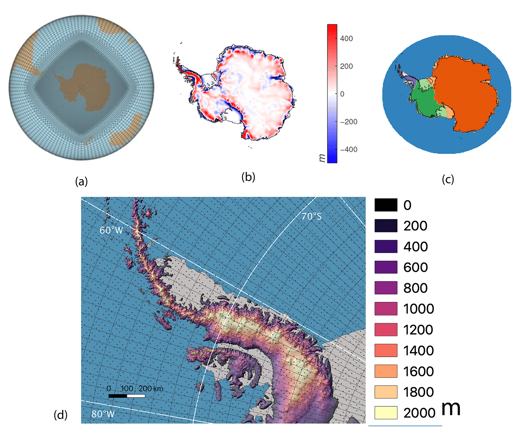
Figure 1Elevation on (a) the ANTSI grid with 0.25∘ spectral element points in the interior and 1∘ in the exterior. (b) Difference between interpolated surface elevation (ANTSI–AMIP) (c) regions shown for East Antarctica (orange), West Antarctica (green), and the Antarctic Peninsula (purple), with lighter shades indicating ice shelves and darker shades indicating the grounded ice sheet; from Zwally et al. (2002). (d) Elevation (source: ETOPO) with the AMIP grid shown by lines and ANTSI spectral element points shown as dots over the Antarctic Peninsula.
2.1.1 The ANTSI grid
The ANTSI (ANTarctic Sea Ice) grid (Fig. 1a) is implemented in CESM2.2 with 32 atmospheric layers. The interior domain has a resolution of 0.25∘, with a nominal 1∘ (standard) grid in the exterior and intermediate-resolution points along the boundaries, which extend as far north as 55∘. These simulations use the AMIP setup (Atmospheric Model Intercomparison Project; Gates, 1992), which is a protocol whereby land and atmosphere components freely evolve but use prescribed sea surface temperatures (ERSSTv5 – Huang et al., 2017) and sea ice (HadISST – Rayner et al., 2003), in this case for the period 1979 to 2014.
In addition to the standard monthly outputs, we produce daily and 3-hourly outputs for selected variables for the surface and 3-hourly outputs for selected variables for both the atmosphere and ice sheet surface. These higher-temporal-resolution outputs will be used for future analysis of atmospheric rivers and forcing of firn models. The computational cost is approximately 23 000 core hours per model year (on the NCAR–Wyoming Cheyenne Supercomputer), and the enhanced storage requirements will scale linearly with the number of cells. For example, the standard 1∘ FV grid has 55296 cells, whereas the ANTSI grid contains 117 398 grid cells (thus requiring roughly double the storage of a 1∘ model).
Elevation over Antarctica (Fig. 1b) is highest in the interior and highly variable at the margins, and ANTSI captures finer resolution than the 1∘ FV grid over both the ocean and ice sheet. Thus, the enhanced resolution of ANTSI better captures topography along the coasts, with some regions of the grounded ice sheet resolving over 400 m higher at the ice sheet margin (e.g., the spine of the Antarctic Peninsula), while ice shelves show slightly lower elevations (Fig. 1b and d).
2.1.2 CESM2 AMIP (GOGA) – used for evaluation
This evaluation primarily focuses on a comparison of ANTSI with the Global Atmosphere–Global Ocean (GOGA) ensemble, a 10-member set of 1∘ prescribed sea surface temperature (SST) experiments with CAM6 conducted by the CESM Climate Variability and Change Working Group (https://www2.cesm.ucar.edu/working_groups/CVC/simulations/cam6-prescribed_sst.html, last access: 10 January 2022) that generally follows what is commonly referred to as the “AMIP” experimental design. In GOGA–AMIP (hereafter referred to as AMIP for short), time-varying SSTs and sea ice concentration are taken from observations, namely ERSSTv5 (Huang et al., 2017) and HadiSST (Rayner et al., 2003), respectively. External radiative forcings use the CMIP6 historical protocol (Eyring et al., 2016) similarly to our ANTSI experiment. For most of our evaluation, we use the ensemble mean of AMIP, except as noted below.
One difference between AMIP and ANTSI that could be important for our evaluation is the dynamical cores of CAM6; ANTSI uses SE, while AMIP uses FV. While it is beyond the scope of this work (and our resources) to conduct a full AMIP-style ensemble with CAM6 and the SE dynamical core, we did conduct two one-member runs with the FV and SE dynamical cores for the 1979–1998 period in the course of model development of the VR-CESM2 (Herrington et al., 2022). These runs are compared and discussed in Sect. 3.3.3 in order to help determine whether differences between ANTSI and GOGA are due to the dynamical core or resolution.
2.1.3 Calculation of surface mass balance
Surface mass balance (SMB, in gigatons, or Gt yr−1) is calculated for both AMIP and ANTSI as follows (adapted from Lenaerts et al., 2019).
We note that the “refreezing” and “retention” terms apply to both “melt” and “rainfall”. For integrated surface mass balance elements as well as snowmelt comparisons, we remap from the finer-resolution grid to the coarser-resolution grid using the Earth System Modeling Framework (ESMF, described at http://earthsystemmodeling.org/, last access: 7 January 2022) using the first-order conservative method and accounting for the percentage of the grid cell that is covered by glacier.
For all other comparisons, in order to preserve the spatial characteristics of the finer resolution, we regrid from a lower resolution to the finer ANTSI resolution using the ESMF bilinear method. The ice sheet mask is provided by Zwally et al. (2002).
2.2 Datasets used for evaluation
We compare surface mass balance values to those from RACMO2.3p2 (van Wessem et al., 2018). RACMO2.3p2 is a hydrostatic regional climate model (RCM) forced at the boundaries with ERA-Interim, with a multi-layer snow scheme (Ettema et al., 2010), a drifting snow scheme across the ice sheet (Lenaerts et al., 2010, 2012), a sophisticated albedo scheme (Kuipers Munneke et al., 2011), and orography derived from Bamber et al. (2009).
Monthly averaged ERA5 (Hersbach et al., 2020) data are used here for the 1979–2014 period for near-surface temperature, wind, and energy balance components, as well as temperature, geopotential height, moisture, and wind profiles over the Southern Ocean. This dataset assimilates observations into a numerical weather prediction model, producing data at an hourly resolution from 1950 to the present, a horizontal resolution of 31 km, 139 vertical levels (to 1 Pa), and an assimilation of several data products for an elevation (Copernicus Climate Change Service, 2017).
For temperature, we note that ERA5 has been shown to exhibit a slight cold bias in winter in comparison to automatic weather station (AWS) data (except the Antarctic Peninsula) and a warm bias in summer (except West Antarctica) (Zhu et al., 2021).
AWS observations are used here for near-surface temperature and wind speed, retrieved from a collection of 133 AWSs previously evaluated over the AIS (Gossart et al., 2019). These were limited to stations where more than 10 years of near-surface temperatures and wind speeds were available and where elevation differences between the station and the resolved elevation (from either AMIP or ANTSI) were smaller than 100 m. Additionally, we apply a temperature adjustment to the AMIP or ANTSI elevation for each AWS using a temperature lapse rate of 6.8 ∘C km−1 (Martin and Peel, 1978). This final set is divided into bins for elevation, with 21 stations >500 m, 1 station between 500 and 1000 m above sea level (a.s.l.), 3 stations between 1000 and 2000 m, 8 stations between 2000 and 3000 m, and 4 stations above 3000 m.
For comparisons to melt observations, we use melt fluxes empirically calculated from radar backscatter from the QuikSCAT (QSCAT) satellite (Trusel et al., 2013), available at 27.2 km2. For comparisons to surface mass balance, we use the AIS SMB reconstruction from Medley and Thomas (2019), which interpolates ice core SMB records based on covariance patterns in atmospheric reanalysis (here using the MERRA2 version of their reconstruction).
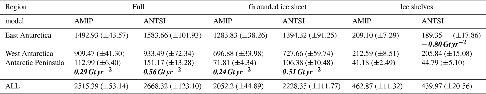
Table 1Surface mass balance values (in Gt yr−1) for each region; the model source is as listed. Interannual trends are shown in bold italic using the Mann–Kendall test where p values are <0.05.
3.1 Surface mass balance
3.1.1 Integrated values for surface mass balance
SMB is lowest in the high elevations of the AIS desert interior, where storms rarely penetrate, and much higher at the coastal margins (Mottram et al., 2021). ANTSI annual mean (1979–2014) AIS integrated SMB is 2668 Gt yr−1, with a temporal standard deviation of 123 Gt yr−1, compared to the AMIP SMB mean over the same period of 2515 Gt yr−1, with an ensemble standard deviation of 53 Gt yr−1. This places integrated ANTSI SMB values within 1 standard deviation of the AMIP SMB mean. This is higher than the 2483 Gt yr−1 ensemble mean calculated for 1979–2018 (the highest calculated being HIRHAM5 0.44 at 2752 Gt yr−1) by Mottram at al. (2021). Regions here (Fig. 1d) are divided by land cover (grounded, ice shelf, combined) and are calculated using basins described in Zwally et al. (2002), with all SMB values and trends listed in Table 1. Mean integrated ANTSI SMB values are slightly higher than, but within 1 standard deviation of, the AMIP ensemble mean for East Antarctica and West Antarctica. ANTSI SMB values for the Antarctic Peninsula are greater than 1 standard deviation for the AMIP mean (151±13 Gt yr−1 for ANTSI vs. 113±6 Gt yr−1 for AMIP), driven by enhanced SMB over the grounded ice sheet (106±10 Gt yr−1 for ANTSI vs. 72±4 Gt yr−1 for AMIP).
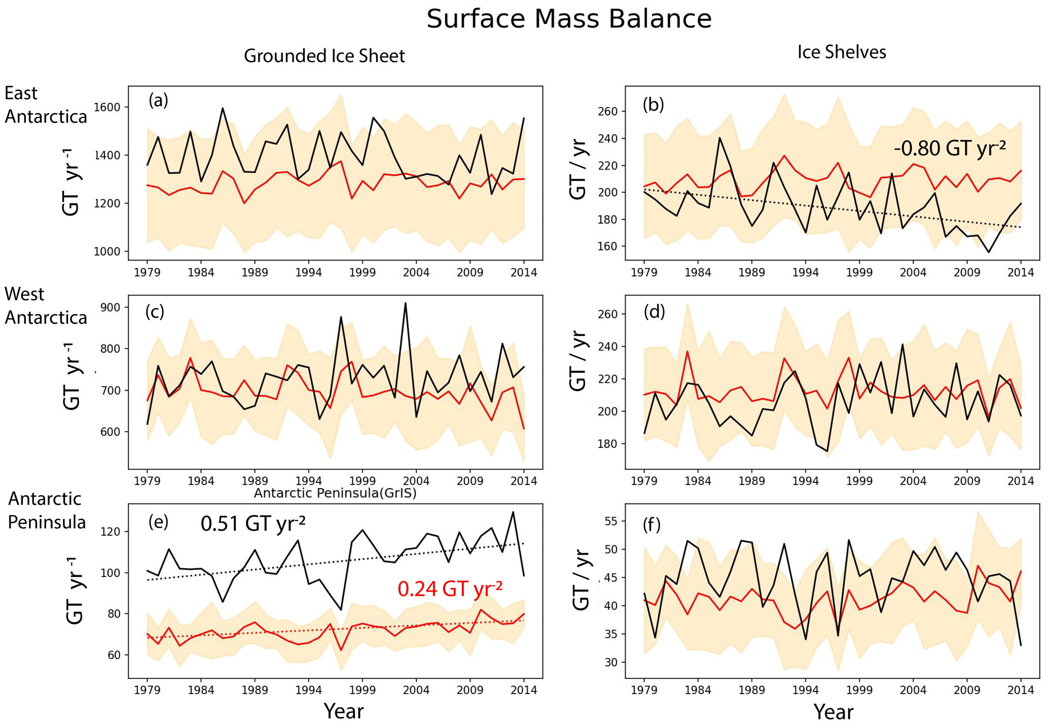
Figure 2Integrated surface mass balance for AMIP (mean shown in orange line, 1 standard deviation shown in orange shade) vs. ANTSI (black line) for (a) the East Antarctic grounded ice sheet, (b) East Antarctic ice shelves, (c) the West Antarctic grounded ice sheet, (d) West Antarctic ice shelves, (e) the Antarctic Peninsula grounded ice sheet, and (f) Antarctic Peninsula ice shelves. Trend lines show where the Mann–Kendall trend test p value <0.05.
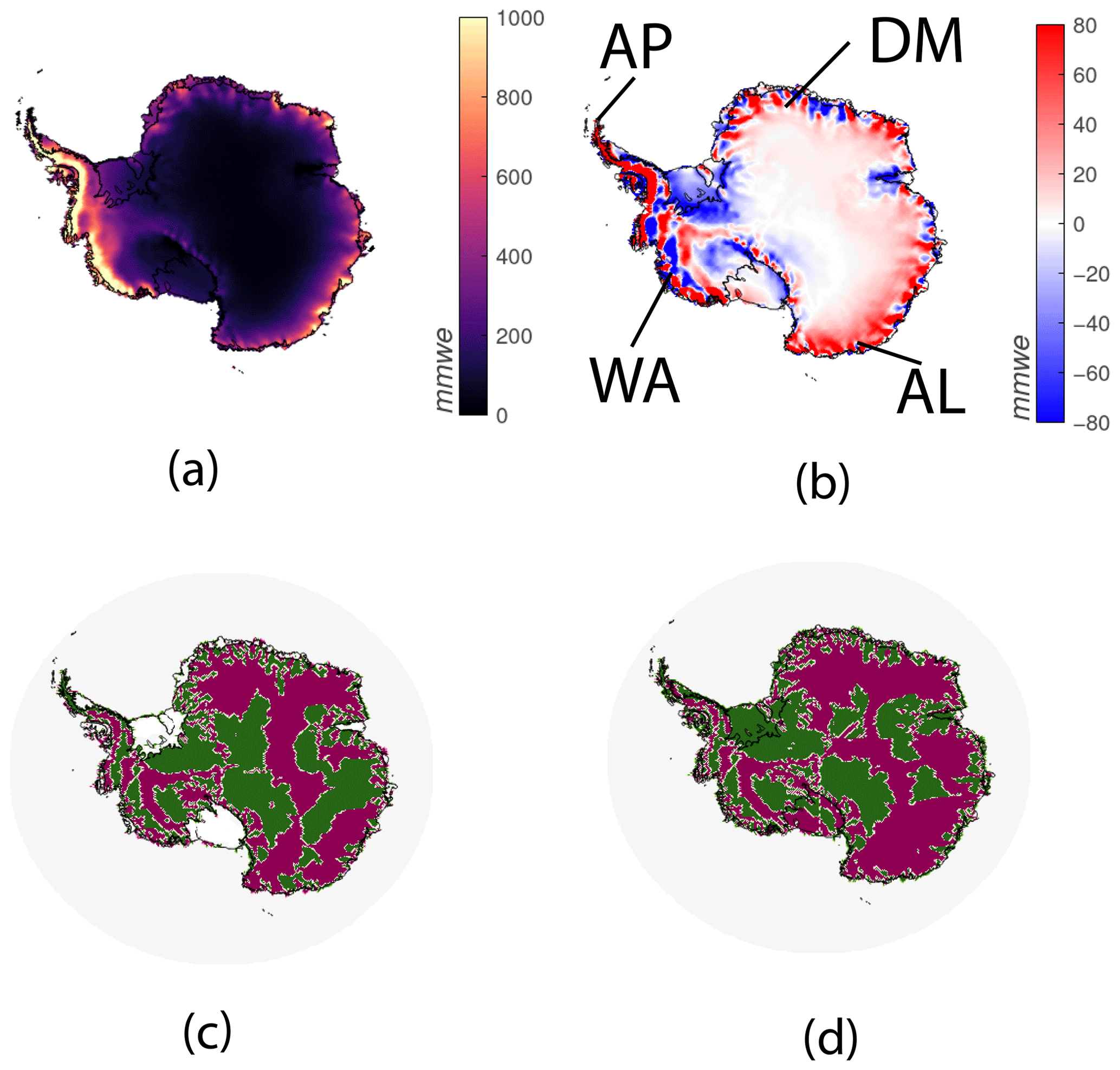
Figure 3Surface mass balance (SMB) over the 1979–2014 period. (a) SMB from ANTSI; (b) difference in SMB (ANTSI–AMIP). Regions indicated include the Antarctic Peninsula (AP), Dronning Maud Land (DM), West Antarctica (WA), and Adélie Land (AL). Panels (c) and (d) show ANTSI SMB bias relative to AMIP compared to the reconstruction and RACM2.3, with green and purple indicating reduced or increased bias in ANTSI relative to the dataset.
Regionally integrated SMB from ANTSI over the 1979–2014 period is provided in Fig. 2. The figure shows several statistically significant (p<0.05) trends, including a −0.80 Gt yr−2 negative trend in SMB over East Antarctic ice shelves which is not replicated by AMIP (Fig. 3b), as well as a positive trend over the grounded ice sheet of the AP for both AMIP (0.24 Gt yr−2) and ANTSI (0.51 Gt yr−2).
3.1.2 Spatial patterns for surface mass balance
The spatial pattern of SMB differences between the higher-resolution ANTSI and the coarser-resolution AMIP (Fig. 3b) results from the interaction between the general atmospheric circulation and elevation differences resulting from enhanced spatial resolution (Fig. 1b). This results in lower SMB values in ANTSI (compared to AMIP) towards the Ronne and Ross ice shelves and greater SMB values in the high interior. In particular, we note differences over the Antarctic Peninsula (AP in Fig. 3b), where SMB values are higher to the west and lower to the east, and West Antarctica (WA in Fig. 3b) where differences occur in regions strongly affected by orographic precipitation (discussed in Sect. 3.2).
To contextualize ANTSI AIS SMB results, we compare SMB results to those calculated from RACMO2.3p2 as well as the SMB reconstruction (Fig. 3c and d). Grounded AIS-integrated SMB values for both AMIP and ANTSI are substantially higher than either RACMO2.3p2, at 1997±92 Gt yr−1, or the reconstruction at 1953±322 Gt yr−1, though there is substantial spatial variability in the differences. Over West Antarctica (denoted WA in Fig. 3b), both comparisons show similar bias patterns, whereby regions where ANTSI SMB estimates are lower show lower biases compared with the reference dataset, and where ANTSI SMB is higher, the bias is worse. Compared with RACMO2.3p2 results (where SMB values are available over ice shelves), results are mixed, with the Ronne, Amery, and Larsen C ice shelves showing better agreement in ANTSI but several other ice shelves (including the Ross ice shelf) showing lower biases with AMIP. Notably, over the Antarctic Peninsula, northern regions near the Larsen C ice shelf typically show lower biases with ANTSI results. While large regions on Dronning Maud Land (DM 30 to 60∘ W) towards the interior show a consistently lower bias in the coarser-resolution AMIP, other regions of East Antarctica show an inconsistent bias increase or reduction between the two reference datasets.
3.1.3 Surface mass balance component: surface melt
Mean spatially integrated surface melt values in ANTSI are similar to AMIP over both the Antarctic Peninsula and West Antarctica (i.e., the ANTSI mean ± 1 standard deviation of the temporal mean overlaps with the AMIP mean ± 1 standard deviation of the ensemble mean). Mean spatially integrated values for regions are shown in Table 1, and temporal plots for spatially integrated values are shown in Fig. 2.
Over East Antarctica, values are significantly higher over ice shelves (ANTSI: 59±20 Gt yr−1, AMIP: 30±4 Gt yr−1), as well as the grounded ice sheet (ANTSI: 34±11 Gt yr−1, AMIP: 11±2 Gt yr−1). Trend analysis (where only significant trends, i.e., p<0.05, are considered) indicates a weak positive trend in AMIP over East Antarctica (0.14 Gt yr−2 over ice shelves, 0.07 Gt yr−2 over the grounded ice sheet) and a weak negative trend over the grounded ice sheet of West Antarctica (−0.09 Gt yr−2). ANTSI shows a stronger positive trend over the ice shelves of the Antarctic Peninsula (0.26 Gt yr−2). In summary, surface melt is intensified within ANTSI on some, but not all, ice shelves. These conflicting biases (despite all ice shelves being resolved to lower elevations in ANTSI) suggest that changes in surface melt are a product of both increased near-surface temperature and changes in atmospheric circulation (both of which can result from enhanced resolution).
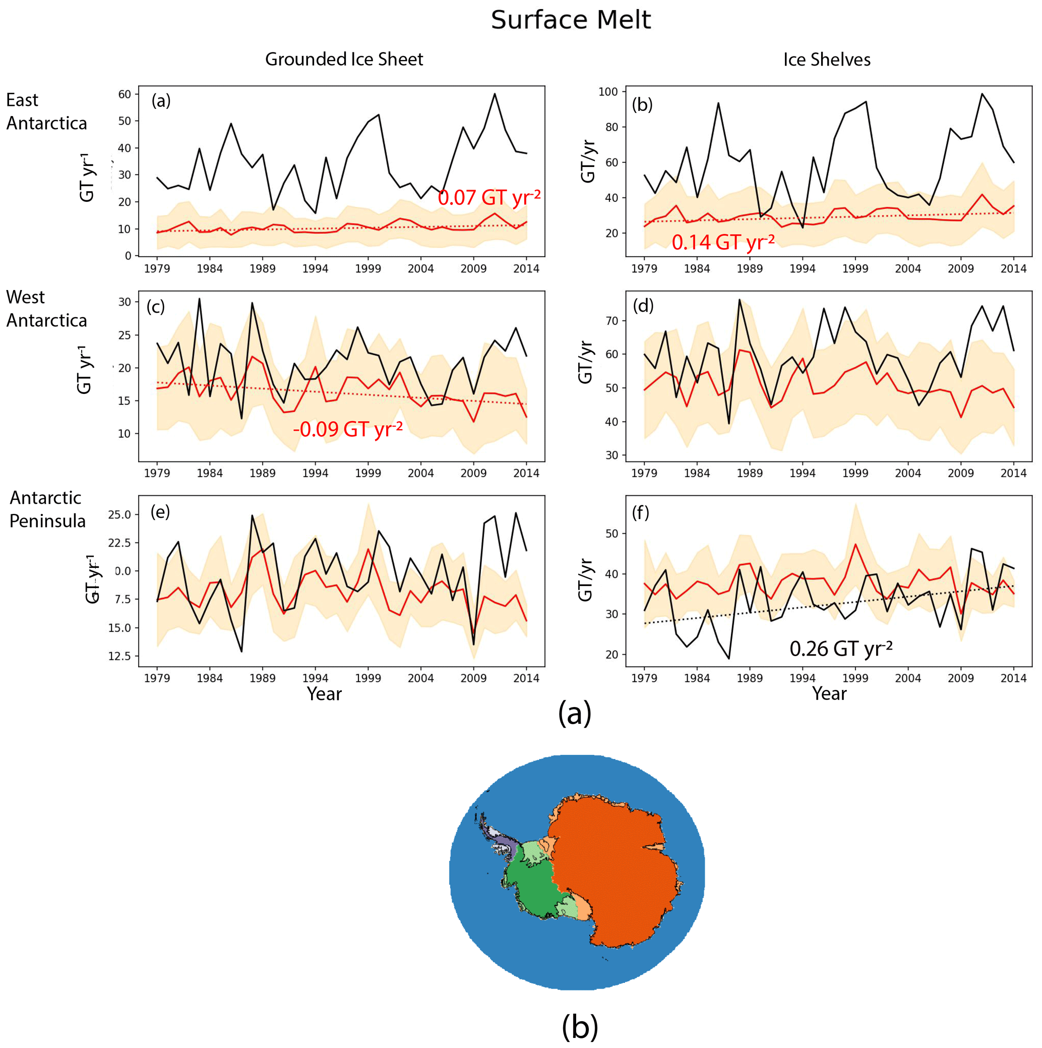
Figure 4(a) Surface melt (in Gt yr−1). (b) Regions for East Antarctica (orange), West Antarctica (green), and the Antarctic Peninsula (purple), with darker colors indicating the grounded ice sheet and lighter colors indicating ice shelves. Based on Zwally et al. (2002).
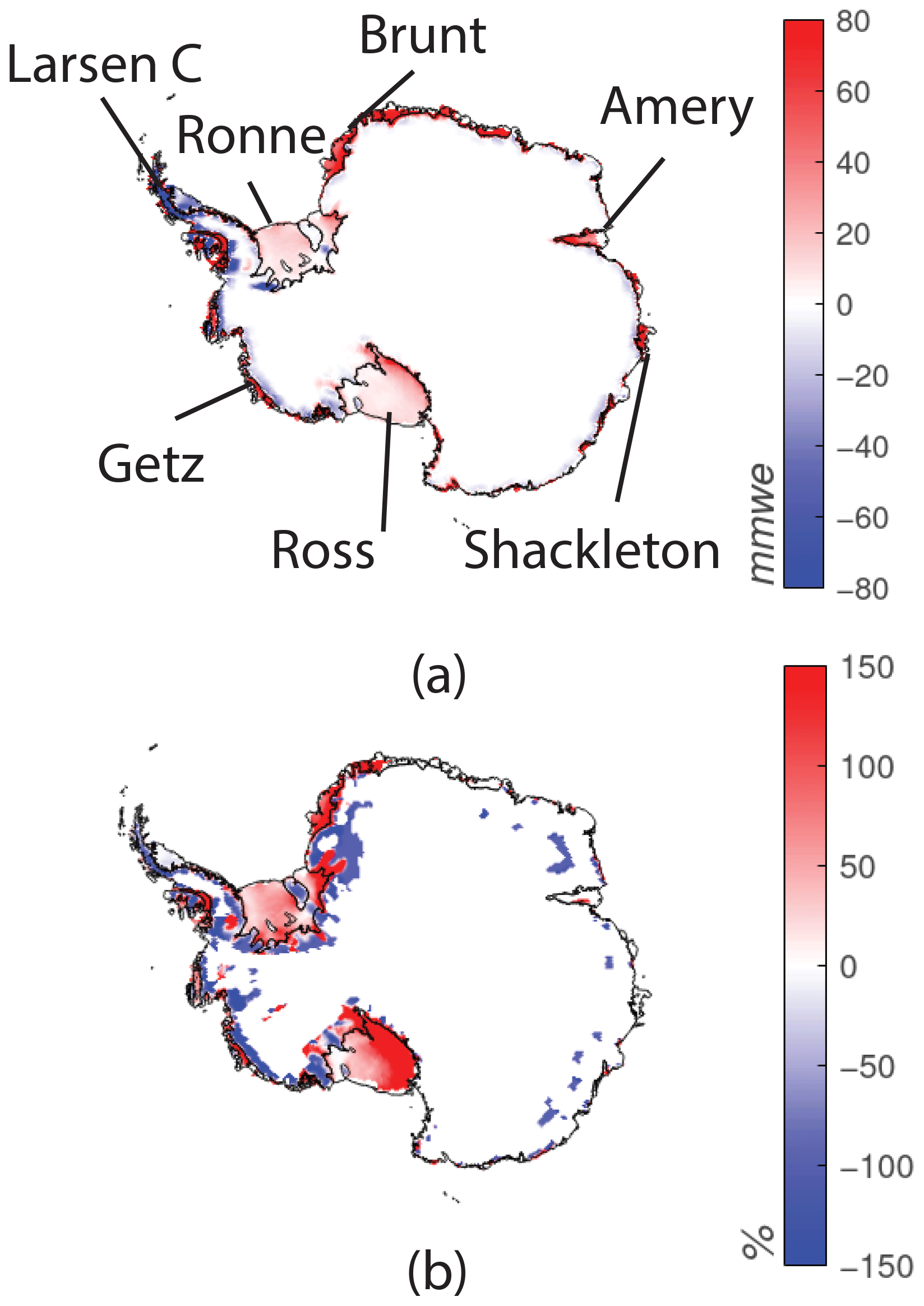
Figure 5Changes in surface melt with resolution. (a) Mean difference in surface melt (ANTSI − AMIP), with individual ice shelves indicated. (b) Restricted to where AMIP surface melt shows a positive bias compared to QSCAT, with red values indicating higher biases. This is the relative difference between models as a percentage, i.e., (ANTSI − AMIP) (AMIP–QSCAT) ⋅ 100.
Compared to AMIP values, mean surface melt in ANTSI is enhanced over the Antarctic Peninsula on the western side but reduced over the eastern side, including the Larsen C ice shelf; this is a direct impact of reduced westerly flow over the AP (discussed further in a later section focused on wind) resulting from the better-resolved topographic barrier. Surface melt is enhanced over much of East Antarctica (Fig. 4a and b) and West Antarctica (Fig. 4c and d) as well, including the Getz, Brunt, Amery, and Shackleton ice shelves (Fig. 5a). However, we note that over the Amery and Shackleton ice shelves, this represents a correction of a negative bias within AMIP, while over most other ice shelves this represents an enhanced positive bias (Fig. 5b).
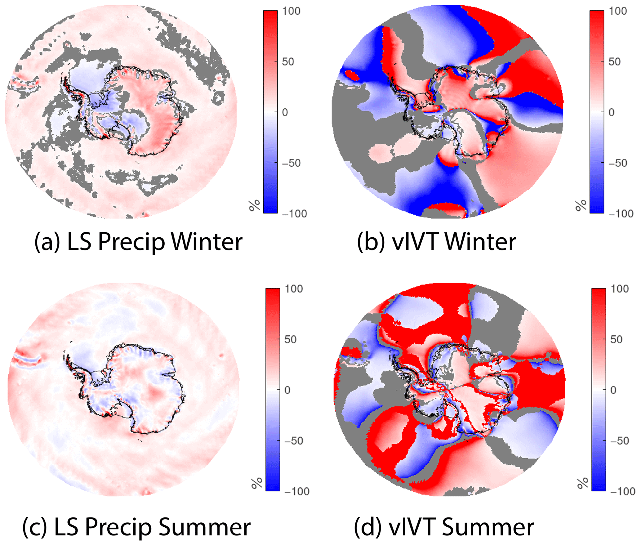
Figure 6Relative change (%) in large-scale (LS) precipitation and integrated meridional vapor transport (vIVT) between ANTSI and AMIP for the 1979–2014 seasonal mean (grey indicates where biases are not significant compared to the AMIP ensemble SD). (a) Large-scale precipitation for winter (JJA) and (c) summer (DJF). Integrated meridional vapor transport for winter (b) and summer (d).
3.2 SMB components: precipitation
Precipitation is the dominant component of SMB over the AIS, and we find that spatial patterns of enhanced or reduced SMB (Fig. 3b) are driven by differences in large-scale precipitation, especially in winter (Fig. 6a), with the summer precipitation contribution to the surplus at higher elevations being smaller than those in winter (Fig. 6c) Over the larger Southern Ocean domain, precipitation is higher in ANTSI than in AMIP (potentially due to the higher resolution in ANTSI), with the exception of the southern Weddell Sea, where the substantially better-resolved (higher) Antarctic Peninsula mountain range in ANTSI inhibits westerly flow and enhances the orographic precipitation gradient between its windward and leeward side. In addition, this enhanced precipitation is partially driven by enhanced meridional vapor transport towards the Weddell Sea sector and much of East Antarctica, especially in winter (Fig. 6b), followed by redistribution driven by enhanced zonal vapor transport in winter (a result of enhanced zonal wind speeds in ANTSI), noting that zonal vapor transport over the ocean is reduced in ANTSI overall (Fig. S3). The atmospheric changes producing this enhanced poleward flow are discussed further in Sect. 3.3.
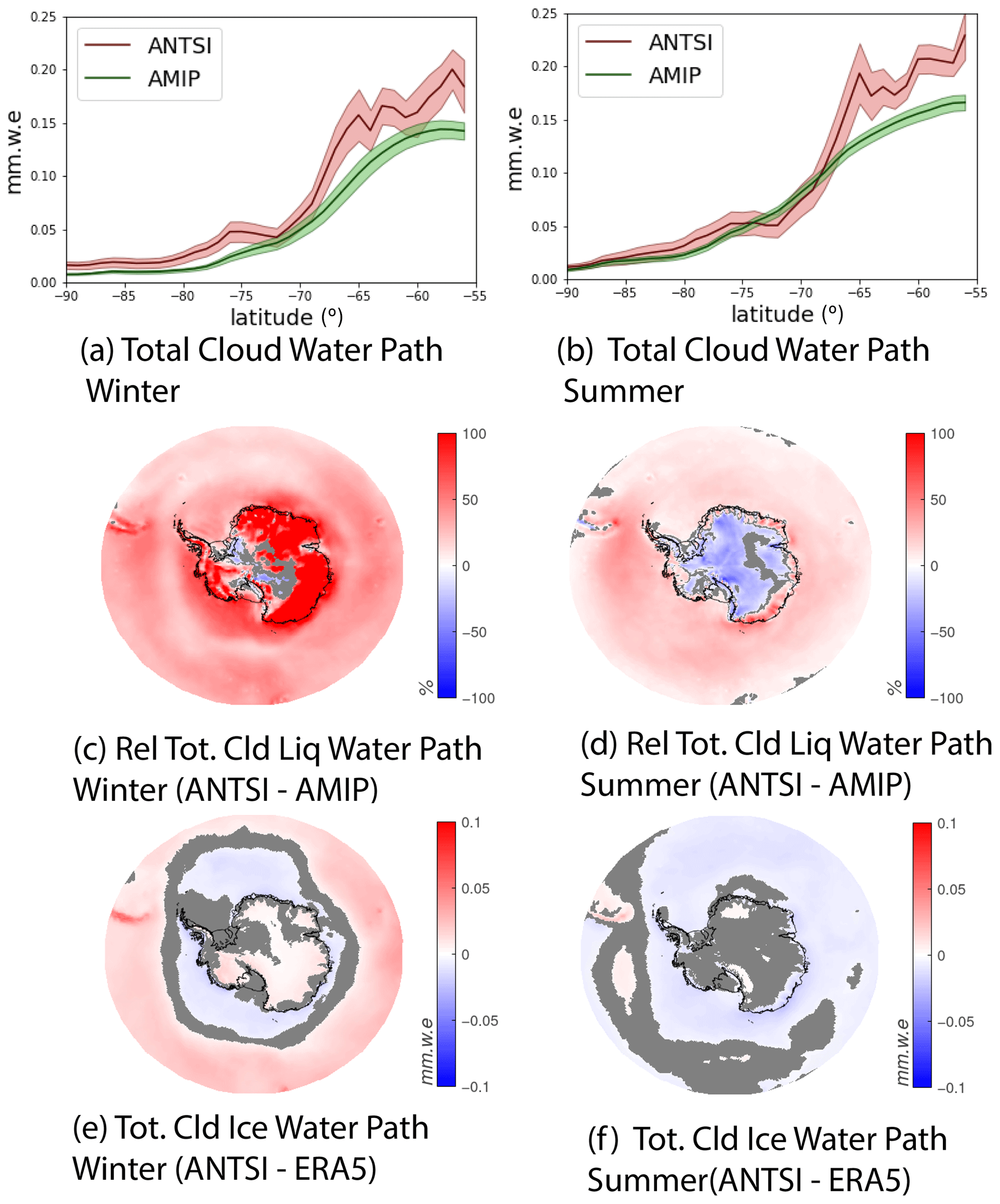
Figure 7Cloud water path. Total cloud water path aggregated in latitude bands (shaded area shows temporal standard deviation) for (a) winter (JJA) and (b) summer (DJF). Relative difference between ANTSI and AMIP (in percentage) in total cloud liquid water path for the seasonal mean (1979–2014) for winter (JJA) (c) and summer (DJF) (d). Absolute difference between ANTSI and ERA5 reanalysis in total cloud ice water path for the seasonal mean (1979–2014) for winter (JJA) (e) and summer (DJF) (f). Grey indicates where biases are not significant compared to the AMIP ensemble SD.
Enhancing resolution resulted in substantial changes to total cloud water path (TCWP, both liquid and ice). TCWP values aggregated by latitude are greater in ANTSI (compared to AMIP) in winter, while in summer, ANTSI values are lower within the 75 to 68∘ S latitude range. This net effect is a combination of changes in both the liquid and ice components, with the biases offsetting each other within the interior of Antarctica during summer. Total liquid cloud water path (TLCWP) is higher in ANTSI vs. AMIP over the larger ocean domain during all seasons (Fig. 7c and d) and over the AIS during winter (Fig. 7c). As lower-resolution AMIP values already showed a high bias compared to ERA5, this represents a further-enhanced bias in ANTSI. However, TLCWP values are smaller in ANTSI over the interior grounded ice sheet during summer (Fig. 6b), and this represents an improvement compared to ERA5 (Fig. S3). Total cloud ice water path (TCIWP) is enhanced by increasing spatial resolution in all seasons, over the ice sheet as well as the interior. As AMIP simulations had a low bias compared to ERA5 estimates (Fig. S3c and i), this amounts to an improvement in the bias over the summer (Fig. 7f), a reversal to a high bias over the interior ice sheet and lower-latitude Southern Ocean, and an improvement over the ocean immediately surrounding the AIS (Fig. 7e).
These results reflect similar spatial patterns in Greenland showing enhanced orographic precipitation in the southeast and drying in the north (van Kampenhout et al., 2019), and we compare these to recent findings in the Discussion (Sect. 4).
3.3 Drivers of enhanced moisture advection
The convergence of precipitation over the AIS is potentially a product of both moisture evaporated over the ocean and changes in winds that transport this moisture poleward. Cloud properties can be affected by the enhanced moisture in the atmosphere. As the Clausius–Clapeyron relationship specifies that the water-holding capacity of air (saturation vapor pressure) increases 7 % with every 1 ∘C of warming (Held and Soden, 2006), even a small change in temperature can strongly affect moisture in the atmosphere and, potentially, cloud cover (though, in the model, the latter is a product of the specific microphysical scheme). In this section, we discuss changes in temperature and wind structure for both winter and summer at the surface and aloft as potential drivers for enhanced moisture advection towards the AIS.
3.3.1 Temperature
Overall, temperatures in ANTSI are higher than AMIP both at the surface and at higher levels in the atmosphere. Biases are higher over the ice sheet than over the ocean, with the strongest biases shown during winter. Where biases are positive during winter over the ice sheet (the majority of the ice sheet), ANTSI biases are 1.76±1.26 ∘C warmer than ERA5 and 2.62±1.27 ∘C warmer than AMIP. Biases during summer are positive over most of the ice sheet and slightly reduced in comparison to winter biases, with winter biases averaging 1.59±1.13 ∘C compared to ERA5 and 1.11±0.68 ∘C compared to AMIP. (Table S2 in the Supplement). Temperature biases at 500 hPa are substantially reduced overall (Table S3).
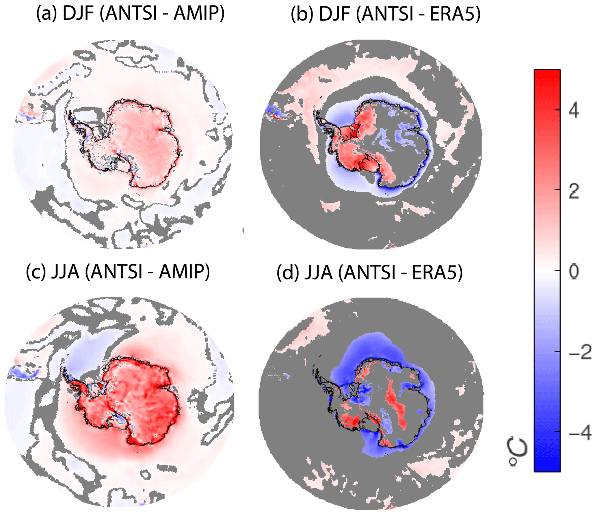
Figure 8Near-surface temperature comparisons between models and reanalysis. (a) DJF ANTSI–AMIP, (b) DJF ANTSI − ERA5, (c) JJA ANTSI–AMIP, and (d) JJA ANTSI–ERA5 where the difference exceeds 1 standard deviation of the AMIP ensemble mean. Grey indicates where biases are not significant compared to the AMIP ensemble SD.
Although temperatures are warmer overall, several regions are cooler, i.e., over the ocean at lower latitudes and to the east of the Antarctic Peninsula, including the Weddell Sea region (Fig. 8a and c). This pattern is likely driven by the enhanced blocking of the AP, which likely produces the precipitation differences shown in Fig. 6a. Compared to ERA5 values in summer, the warmer atmosphere in ANTSI (Fig. 8b) reduces a cold bias present in AMIP (Fig. S4o) over the interior East Antarctic Ice Sheet and the ocean surrounding the AIS. However a warm bias in AMIP is slightly enhanced in ANTSI over the West Antarctic Ice Sheet and the regions of the East Antarctic Ice Sheet nearest to it. Higher winter temperatures in ANTSI reduce a strong cool bias in AMIP (Fig. S5o) compared to ERA5 over both the ocean and ice sheet, even reversing signs to show a warm bias in portions of the East Antarctic interior (Fig. 8d).
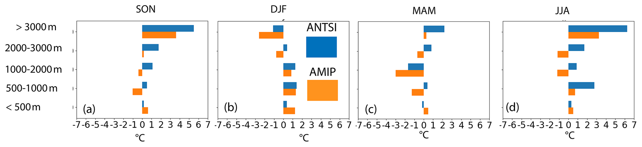
Figure 9Near-surface temperature comparisons with AWSs. Temperature biases compared to AWSs, binned into elevation classes for (a) SON, (b) DJF, (c) MAM, and (d) JJA.
We also examine temperature biases compared to AWSs divided by season and elevation bins (Fig. 9a–d), finding (a) a reduced positive temperature bias in ANTSI compared to larger positive biases in AMIP at elevations <500 m but (b) a warm bias that intensifies with increasing elevation. This results in the partial correction of a cold bias at high elevation during the summer in ANTSI relative to AMIP (Fig. 9). In the winter and shoulder seasons within some higher-elevation areas, the bias changes sign from a cold bias in AMIP to a warm bias in ANTSI. We note that within shoulder seasons and winter, the warm bias at >3000 m elevation is substantially enhanced in SON and JJA. AWS comparisons therefore demonstrate increasing biases with increasing elevation similar to patterns shown in the comparison with ERA5.
The warming produced by enhanced resolution is also shown at lower pressure levels higher in the atmosphere. Comparisons of temperatures at 500 hPa in both summer (Fig. S4p–r) and winter (Fig. S5p–r) show enhanced warming over the entire domain, largely eliminating a cold bias in AMIP (compared to ERA5) over the AIS.
Previous work has discussed how this increase in temperature could be produced, namely by enhanced horizontal spatial resolution enhancing vertical velocities, thus generating greater condensational heating in CLUBB macrophysics within CAM (Herrington and Reed, 2020). Overall, we consider the temperature changes produced by enhanced resolution to be an improvement.
3.3.2 Wind
The near-surface wind climate in Antarctica is governed by higher-speed katabatic winds and a large-scale pressure gradient force (PGF), both of which are stronger in winter (van den Broeke and van Lipzig, 2003).
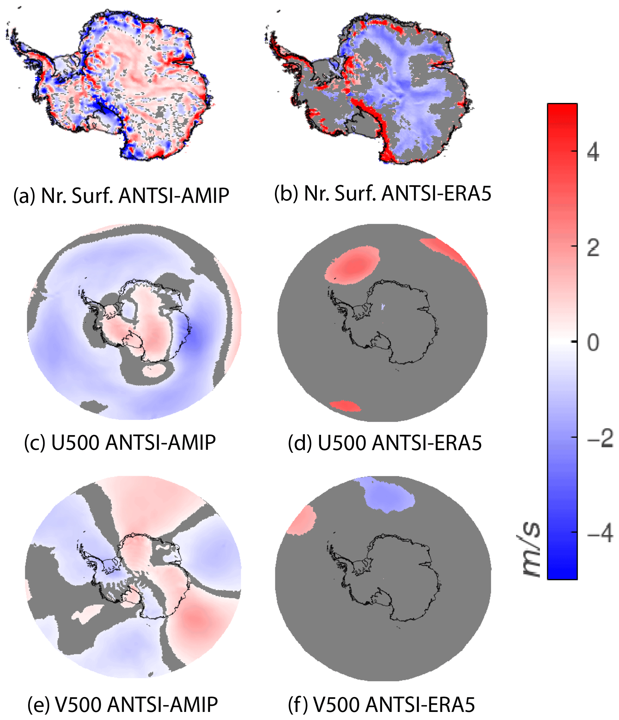
Figure 10Mean winter (JJA) wind speed differences (1979–2014) between ANTSI–AMIP (a, c, e) and ANTSI–ERA5 (b, d, f) for the near surface (a, b), the 500 hPa zonal component (c, d), and the 500 hPa meridional component (e, f). Grey indicates where biases are not significant compared to the AMIP ensemble SD.
Seasonal differences in mean winter wind speed between AMIP vs. ANTSI show enhanced wind speeds in ANTSI where higher elevations are resolved and lower wind speeds on the lee side of the topography (e.g., the East Antarctic peninsula). Generally, negative AMIP biases are improved, but not eliminated, in ANTSI in the interior as well as in the escarpment region, especially in winter (Fig. 10a and b). Where near-surface winter wind speed biases are positive (in comparison to the reference) over the ice sheet, mean ANTSI wind speeds are 1.00±1.13 m s−1 higher than ERA5 and 0.53±0.55 m s−1 higher than AMIP. All other mean biases over the ocean in winter or in summer for either the ocean or ice sheet differ by less than 0.8 m s−1 (Table S3). We note that ANTSI near-surface wind speeds at higher elevations in East Antarctica are higher than AMIP (Fig. 10a) but lower than ERA5 (Fig. 10b). Comparisons between AMIP–ANTSI values and AWSs, binned seasonally and by elevation, show negligible (<1 m s−1) differences for the change in bias (Fig. S6).
To better understand factors contributing to the strong convergence of water vapor over the region, we show a comparison between the meridional and zonal components at 500 hPa, finding that zonal wind speeds are reduced over the ocean, but enhanced in the interior (Fig. 10c), and that meridional wind speeds are higher from the ocean towards the center of East Antarctica. For near-surface as well as meridional and zonal wind speeds at 500 hPa, this represents an overall improvement compared to AMIP simulations (Fig. S5). These improvements are consistent (though less pronounced) in the summer season as well (Fig. S4).
In the aggregate, we find that both temperature and wind fields are improved by enhanced resolution, with the exception of excessive warming in the high interior during winter.
3.3.3 Disambiguating the impacts of dynamical core vs. resolution
The ANTSI and AMIP–GOGA model configurations differ in both spatial resolution and dynamical core. To disambiguate whether the differences are a result of resolution or the dynamical core, we conducted a comparison between runs of two 1∘ versions of CAM6 (one with the FV dynamical core and one with the SE dynamical core, both in a prescribed SST configuration under historical radiative forcing for the 1979–1998 period). We call these the CAM6-FV and CAM6-SE runs, respectively. Since the most notable differences between ANTSI and AMIP–GOGA are total cloud ice and liquid water paths, we compare these variables in the CAM6-FV and CAM6-SE runs, finding no significant differences between them over Antarctica (Fig. S7).
Similarly, to assess the impacts of the dynamical core and resolution on the atmospheric general circulation, we compare the Southern Annular Mode (SAM) and Pacific South American (PSA) patterns among all the model experiments and ERA5 using diagnostic code from the Climate Variability Diagnostics Package (Phillips et al., 2020). The SAM and PSA patterns are widely recognized to be the leading modes of atmospheric circulation variability in the middle and high latitudes of the Southern Hemisphere on monthly to interannual timescales. Significant differences in these modes among the model configurations would have implications for the Antarctic surface mass balance and many other variables. For the AMIP–GOGA ensemble, we ran the diagnostics on each of the 10 ensemble members. For the DJF SAM pattern (Table S5), the spatial pattern correlations and rms differences (compared with ERA5) from CAM6-SE, CAM6-FV, and ANTSI are within the ensemble spread of AMIP–GOGA. In the monthly variability (Fig. S8), the SAM pattern in AMIP–GOGA no. 7 closely resembles the SAM pattern in CAM6-SE. The SAM pattern in AMIP–GOGA no. 5 resembles the SAM pattern in CAM6-FV as well as that in ANTSI. Such inter-ensemble spread in the SAM pattern is to be expected given the large internal variability in the atmospheric circulation. Similar results are obtained for the PSA-1 and PSA-2 patterns (Fig. S9), but this is somewhat complicated by the fact that PSA-1 and PSA-2 can change positions with each other given their similar variance explained (Table S5) and quadrature nature (e.g., Mo and Higgins, 1998). Overall, we do not find major circulation differences between CAM6-SE, CAM6-FV, and ANTSI, and we cannot attribute these differences to the dynamical core or resolution. By extension, the subtle atmospheric circulation differences between ANTSI and AMIP–GOGA are not a good explanation for differences in their SMB or other variables; rather, these differences are likely to be driven by resolution.
3.4 The surface energy budget
The energy available at the surface for melt is described below:
Here, SWnet is net shortwave radiation (SW), LWnet is net longwave radiation (LWdown−LWup), QH is sensible heat transfer, QE is latent heat transfer, QR is the energy supplied by rain, and GR is the energy supplied by ground flux. We have ignored QE, QR, and GR for the purposes of this study, as we expect rain and ground flux to be minimal in Antarctica (Hock, 2005).
In general, ANTSI shows increased LWdown (with resultant impacts on the total energy balance), though this effect is reversed over the ice sheet in summer and accompanied by greater SWnet. Generally, this comprises an improvement in biases compared to ERA5. Although overall changes in the energy balance over the ice sheet are relatively small, the spatial patterns are coherent. All fluxes are defined positively when directed towards the surface, and mean seasonal values for each element of the energy balance are provided as a reference for winter (Fig. S10) and summer (Fig. S11). Additionally, full comparisons of energy balance components comparing values to ERA5 are provided for winter (Fig. S12) and summer (Fig. S13).
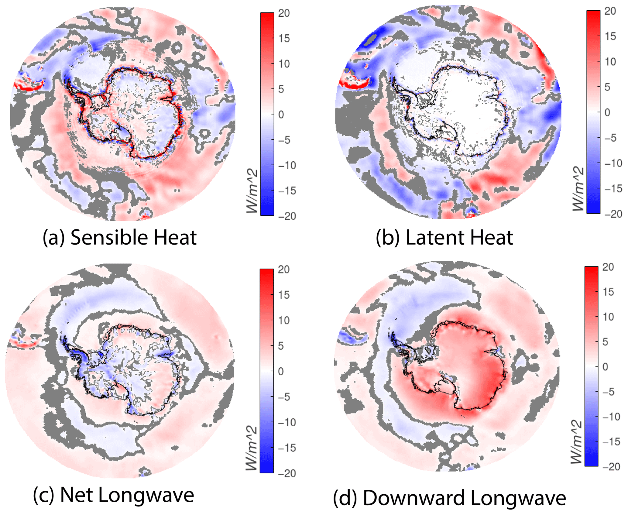
Figure 11Mean differences (ANTSI–AMIP) in the winter (JJA) radiation balance (1979–2014) for (a) sensible heat flux, (b) latent heat flux, (c) net longwave radiation, and (d) downward longwave radiation. All fluxes are directed downward.
3.4.1 Winter
In winter, when incoming shortwave radiation is negligible, net longwave radiation emitted from the surface is a balance between incoming downward and outgoing cooling longwave radiation, with the deficit partially accounted for by changes in sensible heat flux. During winter, ANTSI shows an increase in LWdown over the majority of the continent (Fig. 11d); where biases are positive over the ice sheet, mean winter ANTSI values are 6.78±3.36 W m−2 larger than AMIP (consistent with the warmer atmosphere in ANTSI). However, LWnet shows only a slight increase over East Antarctica and a decrease over much of West Antarctica. Over the ice sheet, positive biases for LWnet average only 1.88±1.57 W m−2, implying an increase in outgoing longwave radiation, which produces the enhanced surface temperatures shown in Fig. 8c. This deficit is partially balanced by compensatory changes in sensible heat flux (Fig. 11a), with a mean positive bias compared to AMIP of 6.12±9.98 W m−2 and a mean negative bias of W m−2.
Over the majority of the ocean domain in winter, ANTSI produces an increase in LWdown (mean positive biases are 2.71±2.67 W m−2), LWnet (mean positive biases are 2.06±2.28 W m−2), and sensible heat flux with positive values directed at the surface (mean positive biases are 3.22±3.87 W m−2, mean negative biases are W m−2), whereas the Amundsen Sea sector and Weddell Sea sector show the reverse of the larger spatial pattern. Latent heat flux is reduced over the larger portion of the ocean (negative biases are W m−2), corresponding to greater latent heat flux from the ocean towards the atmosphere, except sections of the Indian Ocean at lower latitudes.
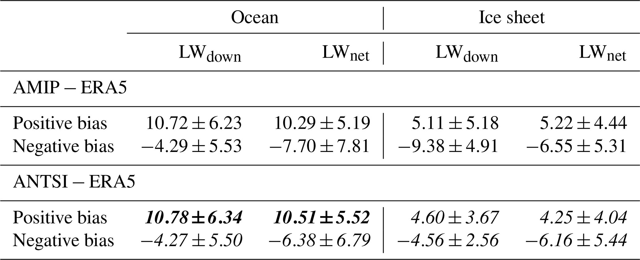
Because sea surface temperature (SSTs) and sea ice concentration (SICs) were forced from observations in this model run, we assume that this behavior is the result of changes in wind patterns and temperature produced by enhanced resolution over the ocean domain. Compared to ERA5 reanalysis, the bias changes in energy balance components in winter are relatively minor except for downward longwave radiation, for which the enhanced resolution produces greater agreement with ERA5 over East Antarctica; the mean negative bias over the ice sheet, compared to ERA5, decreases from W m−2 (AMIP) to W m−2 (ANTSI). The only degradation in winter is a slight increase in mean positive longwave radiation biases (Table 2). We note, in light of the total cloud liquid water path in ANTSI showing greater disagreement with ERA5, that downward longwave radiation is a product of many factors other than cloud liquid water path. In the aggregate, we conclude that the radiation balance in winter is improved with enhanced spatial resolution.
Table 2Mean and standard deviation of downward and net longwave radiation (model − ERA5) in winter (JJA). Values are calculated separately for the sign of bias (positive and negative) and for the ocean (below −55∘ latitude) vs. the ice sheet. Bias improvement is shown in bold italics and degradation in italics.
3.4.2 Summer
In summer (DJF), enhanced LWdown in ANTSI is also greater than in AMIP, though the bias is muted compared to winter, extending over most of the ocean domain except for the Weddell Sea sector and over East Antarctica. Mean summer biases (ANTSI − AMIP) are less than 4 W m−2 over the ocean as well as over the ice sheet. Over the margins of the ice sheet and West Antarctica, LWdown is reduced, partially matching the pattern of reduced total liquid cloud path (Fig. 7b). Over most of the ocean, net longwave radiation and downward longwave radiation are both positive, implying that LWdown is not entirely balanced by longwave cooling (LWup).
Over the majority of the ice sheet, we show a reduction in LWnet, as LWup exceeds the surplus LWdown. LWdown is reduced over the ocean (by nearly 20 W m−2 in regions of the Indian and Pacific sector) and over the center of East Antarctica but greatly increased over the margins as well as the Weddell Sea sector (nearly 15 W m−2 in some regions). The latter is consistent with cloud clearing due to the higher topographic barrier. SWnet decreased substantially over the ocean and increased over the ice sheet.
Table 3Mean and standard deviation of downward and net longwave and shortwave radiation (model − ERA5) in winter (DJF). Values are calculated separately for the sign of bias (positive and negative) and for the ocean (below −55∘ latitude) vs. the ice sheet. Bias improvement is shown in bold italics and degradation in italics.
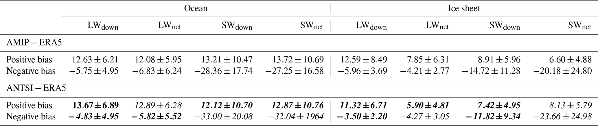
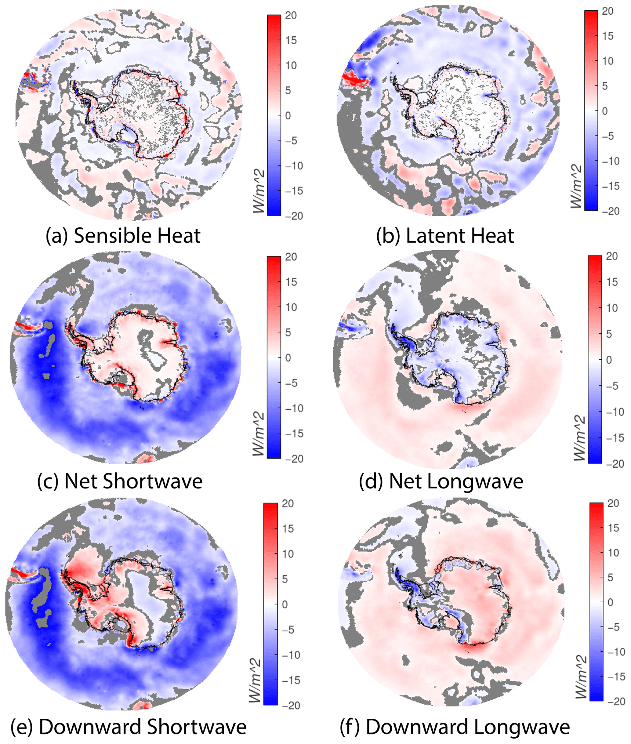
Figure 12Mean differences (ANTSI–AMIP) in the summer (DJF) radiation balance (1979–2014) for (a) sensible heat flux, (b) latent heat flux, (c) net shortwave radiation, (d) net longwave radiation, (e) downward shortwave radiation, and (f) downward longwave radiation. All fluxes are directed downward.
In comparison to ERA5, the biases over oceans for LWdown, LWnet, SWdown, and SWnet increase in ANTSI (Fig. 12, Table 3, Figs. S12 and S13). Over the ice sheet, biases show a distinct spatial pattern, with the bias sign reversing between the high plateau in East Antarctica vs. West Antarctica and the margins of the ice sheet. In the aggregate, the radiation balance is improved or changed only slightly, with mean biases reduced (Table 3) and biases within ANTSI falling within 1 standard deviation of the ERA5 mean (Fig. S13h, i, n, o, q, r). The exception is SWnet (generally a positive bias), for which ANTSI biases are higher overall.
In summary, during summer, the representation of the radiation balance shows reduced biases compared to ERA5 over the ice sheet (with the exception of net shortwave radiation), but over the ocean, biases in both shortwave and longwave radiation increased within ANTSI. One exception to this generalized spatial pattern is the Weddell Sea sector, where the better-resolved (higher) Antarctic Peninsula blocks westerly flow.
In this study, we have compared the climatology in the standard-resolution 1∘ CESM2 with the variable-resolution CESM2, which has high resolution (as fine as 0.25∘) over Antarctica and the Southern Ocean. We find that enhanced horizontal resolution generally reduces climatological biases, except with regard to the formation of clouds over the Southern Ocean. Temperature and wind speed biases (both near the surface and aloft) are largely reduced over both the ocean and the ice sheet, and surface mass balance estimates are generally equivalent, except for over the Antarctic Peninsula. Here, the high resolution resolves the spine of the Antarctic Peninsula mountain range to over 400 m greater height, resulting in enhanced precipitation on the western side and reduced precipitation, lower temperature, and decreased surface melt on the eastern side and the Weddell Sea sector. In comparison to an ice-core-based, gridded reconstruction as well as the regional climate model RACMO2.3p2, SMB biases from both datasets produce similar spatial patterns for changes in bias over the AP, West Antarctica, and some regions of East Antarctica. There is better agreement between the enhanced-resolution model (ANTSI) and the reference datasets over lower-elevation regions in West Antarctica and sections of East Antarctica nearest the Ronne–Filchner and Ross ice shelves, while biases increased over Dronning Maud Land. These changes are primarily driven by greater precipitation in these regions driven by enhanced meridional vapor transport from the oceans, especially in winter.
While temperature, wind (both zonal and meridional), specific humidity, and total cloud ice water path over the ocean are improved, biases are increased for total cloud liquid water path (TCLWP) over the ocean region in both summer and winter, with a concurrent decrease in downward and net shortwave and increase in downward and net longwave in summer. Over the ice sheet, TCLWP biases are higher in winter compared to ERA5, but the increase in downward longwave radiation (partially affected by TCLWP) amounts to a reduction in bias compared to ERA5. By contrast, summer TCLWP is higher at the margins but lower in the interior of the ice sheet, a pattern conforming to changes in orographic precipitation produced by enhanced resolution reported by van Kampenhout et al. (2019). The summer patterns for biases in downward and net longwave and downward shortwave (but not net shortwave) indicate reduced biases. The change in downward shortwave radiation and higher temperatures may cause another bias, namely the increase in surface melt over most ice shelves, except the eastern side of the Antarctic Peninsula (where temperatures are kept lower by the orographic barrier). We note that only for a few ice shelves (such as the Brunt ice shelf and interior of the Ross ice shelf) does this represent a significant relative increase compared to the already high bias between the coarser-resolution AMIP and observations (QuikSCAT). The increased surface melt also represents an improvement in bias compared to QuikSCAT over the Amery and Shackleton ice shelves, where coarser-resolution simulations underpredict surface melt.
Biases are largely reduced in the near-surface atmosphere over the ice sheet and ocean. However, the physics of cloud formation (and resultant precipitation), especially over the ocean, may be better parameterized for the coarser-resolution model. Future improvements to CAM may benefit from examining how parameterizations affect cloud formation over the Southern Ocean in particular, where there are few land masses and where the enhanced availability of precipitation can strongly impact surface mass balance over the ice sheet. Currently, tuning for CESM2 has focused on the standard 1∘ grid, while future parameterizations will account for the effects on variable-resolution grids (including ANTSI). It is also likely that more detailed evaluations of clouds and related properties, employing different observational datasets and cloud simulators, will help to better pinpoint deficiencies in all versions of the model than we have been able to do here with the reanalysis. We also note the possibility that these biases could be alleviated with the activation of the high-resolution ocean component of CESM2, rather than the one-way forced sea surface temperature and sea ice concentration formulation used in these simulations. Notably, recent work employing a global, fully coupled, high-resolution (0.25∘ atmosphere; 0.10∘ ocean) decadal prediction system with CESM1 suggests that high resolution over the Southern Ocean in particular is key for improving climate simulations across the globe (Yeager et al., 2023). However, that work was extremely computationally expensive; a coupled implementation of VR-CESM2 with enhanced resolution over the ANTSI domain might provide similar improvements at much lower expense.
By providing knowledge of its strengths and limitations, this work illustrates that the variable-resolution configuration over Antarctica is a valuable tool for representations of precipitation, surface mass balance, and therefore sea level rise estimates. In particular, the enhanced-resolution better articulates spatial patterns associated with orographic precipitation, which may capture fine-scale changes in precipitation patterns in future warming scenarios. We note that the improvements over Antarctica are less pronounced than those over Greenland, where they are significant (van Kampenhout et al., 2019). The enhanced resolution grid captures these changes while preserving two-way interaction with the global climate system, but at a reduced computational cost compared to global high-resolution runs. However, we note that some regional climate models such as RACMO2.3p2 (van Wessem et al., 2018) and the MAR model (Agosta et al., 2019) contain more detailed representations of the firn layer as well as more complex albedo schemes. Therefore, RCMs and VR ESMs currently serve different purposes. For studies specifically focused on the effects on the two-way interactions with firn, RCMs such as RACMO2.3p2 and MAR may provide better value overall. For these ANTSI runs, we note that outputs have been produced at 3-hourly intervals that could be used to force offline firn models with even finer representation of firn layers than RCMs. Similarly, despite a poorer representation of the firn layer, very-high-resolution nonhydrostatic models (Gilbert et al., 2022) best capture wind and temperature dynamics over the East Antarctic peninsula, e.g., foehn flow. While the variable-resolution domain provides substantial value for experiments fully utilizing the two-way interaction between the interior and global domain, they do not replace RCMs.
Future work will take advantage of the enhanced resolution and relatively low computational cost of ANTSI. While our evaluation of ANTSI has focused on the 1979–2014 period (to match available AMIP results), results from ANTSI are available for the 2015–2020 period, for which we have implemented moisture tagging, connecting precipitation to its sources. As infrequent and sometimes small-spatial-scale extreme events constitute a substantial fraction of mean annual precipitation over much of the Antarctic Ice Sheet (Dalaiden et al., 2020), high resolution will offer better insights into their dynamics and impacts. In future work, we will use ANTSI to present the climatology and moisture sources of atmospheric rivers over the Antarctic Ice Sheet. We also anticipate the use of the ANTSI grid in fully coupled runs for future climate scenarios, better constraining the dynamics of precipitation over the Antarctic Ice Sheet and thus future estimates of sea level rise.
All outputs used for this evaluation are available through Zenodo: https://doi.org/10.5281/zenodo.7335892 (Datta, 2022).
The supplement related to this article is available online at: https://doi.org/10.5194/tc-17-3847-2023-supplement.
RTD performed simulations and major analysis. AH provided substantial guidance about the usage of VR-CESM2. JTML provided initial guidance on the project design. DPS provided input on the analysis and on the final version of the paper. ZY and LT provided input on the final paper. DD provided input on initial versions of the paper.
The contact author has declared that none of the authors has any competing interests.
Publisher's note: Copernicus Publications remains neutral with regard to jurisdictional claims in published maps and institutional affiliations.
Funding for this work, through Rajashree Tri Datta, Jan T. M. Lenaerts, David P. Schneider, Devon D. Dunmire, and Ziqi Yin, was provided by grant 1952199 from the National Science Foundation (NSF), Office of Polar Programs. Rajashree Tri Datta and Luke Trusel also received funding through NASA grant S000885; David P. Schneider was also supported through the National Center for Atmospheric Research, which is a major facility sponsored by the NSF, under cooperative agreement no. 1852977. The authors thank all the scientists, software engineers, and administrators who contributed to the development of CESM, which is primarily supported by the NSF. Finally, the authors appreciate the efforts of the reviewers and editors, whose constructive comments led to an improved paper.
This research has been supported by the National Science Foundation (grant no. OPP 1952199) and the National Aeronautics and Space Administration (grant no. S000885-NASA).
This paper was edited by Ruth Mottram and reviewed by Ella Gilbert and one anonymous referee.
Agosta, C., Amory, C., Kittel, C., Orsi, A., Favier, V., Gallée, H., van den Broeke, M. R., Lenaerts, J. T. M., van Wessem, J. M., van de Berg, W. J., and Fettweis, X.: Estimation of the Antarctic surface mass balance using the regional climate model MAR (1979–2015) and identification of dominant processes, The Cryosphere, 13, 281–296, https://doi.org/10.5194/tc-13-281-2019, 2019.
Bambach, N. E., Rhoades, A. M., Hatchett, B. J., Jones, A. D., Ullrich, P. A., and Zarzycki, C. M.: Projecting climate change in South America using variable-resolution Community Earth System Model: An application to Chile, Int. J. Climatol., 42, 2514–254, https://doi.org/10.1002/joc.7379, 2022.
Bamber, J. L., Gomez-Dans, J. L., and Griggs, J. A.: A new 1 km digital elevation model of the Antarctic derived from combined satellite radar and laser data – Part 1: Data and methods, The Cryosphere, 3, 101–111, https://doi.org/10.5194/tc-3-101-2009, 2009.
Banwell, A. F., MacAyeal, D. R., and Sergienko, O. V.: Breakup of the Larsen B Ice Shelf triggered by chain reaction drainage of supraglacial lakes, Geophys. Res. Lett., 40, 5872–5876, https://doi.org/10.1002/2013GL057694, 2013.
Copernicus Climate Change Service (C3S): ERA5: Fifth generation of ECMWF atmospheric reanalyses of the global climate, Copernicus Climate Change Service Climate Data Store (CDS), 10/2022, https://cds.climate.copernicus.eu/cdsapp#!/home (last access: 10 January 2022), 2017.
Dalaiden, Q., Goosse, H., Lenaerts, J. T. M., Cavitte, M. G. P., and Henderson, N.: Future Antarctic snow accumulation trend is dominated by atmospheric synoptic-scale events, Commun. Earth Environ., 1, 62, https://doi.org/10.1038/s43247-020-00062-x, 2020.
Danabasoglu, G., Lamarque, J.-F., Bacmeister, J., Bailey, D. A., DuVivier, A. K., Edwards, J., Emmons, L. K., Fasullo, J., Garcia, R., Gettelman, A., Hannay, C., Holland, M. M., Large, W. G., Lauritzen, P. H., Lawrence, D. M., Lenaerts, J. T. M., Lindsay, K., Lipscomb, W. H., Mills, M. J., Neale, R., Oleson, K. W. , Otto-Bliesner, B., Phillips, A. S., Sacks, W., Tilmes, S., van Kampenhout, L., Vertenstein, M., Bertini, A., Dennis, J., Deser, C., Fischer, C., Fox-Kemper, B., Kay, J. E., Kinnison, D., Kushner, P. J., Larson, V. E., Long, M. C., Mickelson, S., Moore, J. K., Nienhouse, E., Polvani, L., Rasch, P. J., and Strand, W. G.: The Community Earth System Model Version 2 (CESM2), J. Adv. Model. Earth Sy., 12, e2019MS001916, https://doi.org/10.1029/2019MS001916, 2020.
Datta, R.: Variable-resolution CESM2 over Antarctica (ANTSI): Monthly outputs used for evaluation, Zenodo [data set], https://doi.org/10.5281/zenodo.7335892, 2022.
Dennis, J. M., Edwards, J., Evans, K. J., Guba, O., Lauritzen, P. H., Mirin, A. A., St-Cyr, A., Taylor, M. A., and Worley, P. H.: CAM-SE: A scalable spectral element dynamical core for the Community Atmosphere Model, Int. J. High Perform. C., 26, 74–89, https://doi.org/10.1177/1094342011428142, 2012.
Dunmire, D., Lenaerts, J. T. M., Datta, R. T., and Gorte, T.: Antarctic surface climate and surface mass balance in the Community Earth System Model version 2 during the satellite era and into the future (1979–2100), The Cryosphere, 16, 4163–4184, https://doi.org/10.5194/tc-16-4163-2022, 2022.
Ettema, J., van den Broeke, M. R., van Meijgaard, E., van de Berg, W. J., Box, J. E., and Steffen, K.: Climate of the Greenland ice sheet using a high-resolution climate model – Part 1: Evaluation, The Cryosphere, 4, 511–527, https://doi.org/10.5194/tc-4-511-2010, 2010.
Eyring, V., Bony, S., Meehl, G. A., Senior, C. A., Stevens, B., Stouffer, R. J., and Taylor, K. E.: Overview of the Coupled Model Intercomparison Project Phase 6 (CMIP6) experimental design and organization, Geosci. Model Dev., 9, 1937–1958, https://doi.org/10.5194/gmd-9-1937-2016, 2016.
Gates, W. L.: AMIP: The Atmospheric Model Intercomparison Project, B. Am. Meteorol. Soc., 73, 1962–1970, 1992.
Gettelman, A., Hannay, C., Bacmeister, J. T., Neale, R. B., Pendergrass, A. G., Danabasoglu, G., Lamarque, J.-F., Fasullo, J. T., Bailey, D. A., Lawrence, D. M., and Mills, M. J.: High Climate Sensitivity in the Community Earth System Model Version 2 (CESM2), Geophys. Res. Lett., 46, 8329–8337, https://doi.org/10.1029/2019GL083978, 2019.
Gilbert, E. and Kittel, C.: Surface Melt and Runoff on Antarctic Ice Shelves at 1.5 ∘C, 2 ∘C, and 4 ∘C of Future Warming, Geophys. Res. Lett., 48, e2020GL091733, https://doi.org/10.1029/2020GL091733, 2021.
Gilbert, E., Orr, A., Renfrew, I. A., King, J. C., and Lachlan-Cope, T.: A 20-Year Study of Melt Processes Over Larsen C Ice Shelf Using a High-Resolution Regional Atmospheric Model: 2. Drivers of Surface Melting, J. Geophys. Res.-Atmos., 127, e2021JD036012, https://doi.org/10.1029/2021JD036012, 2022.
Gossart, A., Helsen, S., Lenaerts, J. T. M., Broucke, S. V., van Lipzig, N. P. M., and Souverijns, N.: An Evaluation of Surface Climatology in State-of-the-Art Reanalyses over the Antarctic Ice Sheet, J. Climate, 32, 6899–6915, https://doi.org/10.1175/JCLI-D-19-0030.1, 2019.
Held, I. M. and Soden, B. J.: Robust Responses of the Hydrological Cycle to Global Warming, J. Climate, 19, 5686–5699, https://doi.org/10.1175/JCLI3990.1, 2006.
Herrington, A. R. and Reed, K. A.: On resolution sensitivity in the Community Atmosphere Model, Q. J. Roy. Meteor. Soc., 146, 3789–3807, https://doi.org/10.1002/qj.3873, 2020.
Herrington, A. R., Lauritzen, P. H., Lofverstrom, M., Lipscomb, W. H., Gettelman, A., and Taylor, M. A.: Impact of grids and dynamical cores in CESM2.2 on the surface mass balance of the Greenland Ice Sheet, J. Adv. Model. Earth Sy., 14, e2022MS003192, https://doi.org/10.1029/2022MS003192, 2022.
Hersbach, H., Bell, B., Berrisford, P., Hirahara, S., Horányi, A., Muñoz-Sabater, J., Nicolas, J., Peubey, C., Radu, R., Schepers, D., Simmons, A., Soci, C., Abdalla, S., Abellan, X., Balsamo, G., Bechtold, P., Biavati, G., Bidlot, J., Bonavita, M., De Chiara, G., Dahlgren, P., Dee, D., Diamantakis, M., Dragani, R., Flemming, J., Forbes, R., Fuentes, M., Geer, A., Haimberger, L., Healy, S., Hogan, R. J., Hólm, E., Janisková, M., Keeley, S., Laloyaux, P., Lopez, P., Lupu, C., Radnoti, G., de Rosnay, P., Rozum, I., Vamborg, F., Villaume, S., and Thépaut, J.-N.: The ERA5 global reanalysis, Q. J. Roy. Meteor. Soc., 146, 1999–2049, https://doi.org/10.1002/qj.3803, 2020.
Hock, R.: Glacier melt: A review of processes and their modelling, Prog. Phys. Geogr., 29, 362–391, https://doi.org/10.1191/0309133305pp453ra, 2005.
Huang, B., Thorne, P. W., Banzon, V. F., Boyer, T., Chepurin, G., Lawrimore, J. H., Menne, M. J., Smith, T. M., Vose, R. S., and Zhang, H.-M.: Extended Reconstructed Sea Surface Temperature, Version 5 (ERSSTv5): Upgrades, Validations, and Intercomparisons, J. Climate, 30, 8179–8205, https://doi.org/10.1175/JCLI-D-16-0836.1, 2017.
Huang, X., Rhoades, A. M., Ullrich, P. A., and Zarzycki, C. M.: An evaluation of the variable-resolution CESM for modeling California's climate, J. Adv. Model. Earth Sy., 8, 345–369, https://doi.org/10.1002/2015MS000559, 2016.
Hulbe, C. L., Scambos, T. A., Youngberg, T., and Lamb, A. K.: Patterns of glacier response to disintegration of the Larsen B ice shelf, Antarctic Peninsula, Global Planet. Change, 63, 1–8, https://doi.org/10.1016/j.gloplacha.2008.04.001, 2008.
Hunke, E. and Lipscomb, W.: CICE: The Los Alamos sea ice model documentation and software user's manual version 4.0 LA-CC-06-012, Tech. Rep. LA-CC-06-012, 2010.
Intergovernmental Panel on Climate Change (IPCC) (Ed.): Sea Level Rise and Implications for Low-Lying Islands, Coasts and Communities, in: The Ocean and Cryosphere in a Changing Climate: Special Report of the Intergovernmental Panel on Climate Change, Cambridge University Press, Cambridge Cor, 321–446, https://doi.org/10.1017/9781009157964.006, 2022.
Kittel, C., Amory, C., Agosta, C., Jourdain, N. C., Hofer, S., Delhasse, A., Doutreloup, S., Huot, P.-V., Lang, C., Fichefet, T., and Fettweis, X.: Diverging future surface mass balance between the Antarctic ice shelves and grounded ice sheet, The Cryosphere, 15, 1215–1236, https://doi.org/10.5194/tc-15-1215-2021, 2021.
Krinner, G. and Genthon, C.: The Antarctic surface mass balance in a stretched grid general circulation model, Ann. Glaciol., 25, 73–78, https://doi.org/10.3189/S0260305500013823, 1997.
Krinner, G., Genthon, C., Li, Z.-X., and Le Van, P.: Studies of the Antarctic climate with a stretched-grid general circulation model, J. Geophys. Res.-Atmos., 102, 13731–13745, https://doi.org/10.1029/96JD03356, 1997.
Krinner, G., Magand, O., Simmonds, I., Genthon, C., and Dufresne, J.-L.: Simulated Antarctic precipitation and surface mass balance at the end of the twentieth and twenty-first centuries, Clim. Dynam., 28, 215–230, https://doi.org/10.1007/s00382-006-0177-x, 2007.
Krinner, G., Largeron, C., Ménégoz, M., Agosta, C., and Brutel-Vuilmet, C.: Oceanic Forcing of Antarctic Climate Change: A Study Using a Stretched-Grid Atmospheric General Circulation Model, J. Climate, 27, 5786–5800, https://doi.org/10.1175/JCLI-D-13-00367.1, 2014.
Kuipers Munneke, P., van den Broeke, M. R., Lenaerts, J. T. M., Flanner, M. G., Gardner, A. S., and van de Berg, W. J.: A new albedo parameterization for use in climate models over the Antarctic ice sheet, J. Geophys. Res.-Atmos., 116, D05114, https://doi.org/10.1029/2010JD015113, 2011.
Lauritzen, P. H., Nair, R. D., Herrington, A. R., Callaghan, P., Goldhaber, S., Dennis, J. M., Bacmeister, J. T., Eaton, B. E., Zarzycki, C. M., Taylor, M. A., Ullrich, P. A., Dubos, T., Gettelman, A., Neale, R. B., Dobbins, B., Reed, K. A., Hannay, C., Medeiros, B., Benedict, J. J., and Tribbia, J. J.: NCAR Release of CAM-SE in CESM2.0: A Reformulation of the Spectral Element Dynamical Core in Dry-Mass Vertical Coordinates With Comprehensive Treatment of Condensates and Energy, J. Adv. Model. Earth Sy., 10, 1537–1570, https://doi.org/10.1029/2017MS001257, 2018.
Lawrence, D. M., Oleson, K. W., Flanner, M. G., Thornton, P. E., Swenson, S. C., Lawrence, P. J., Zeng, X., Yang, Z.-L., Levis, S., Sakaguchi, K., Bonan, G. B., and Slater, A. G.: Parameterization improvements and functional and structural advances in Version 4 of the Community Land Model, J. Adv. Model. Earth Sy., 3, M03001, https://doi.org/10.1029/2011MS00045, 2011.
Lenaerts, J. T. M., van den Broeke, M. R., Déry, S. J., König-Langlo, G., Ettema, J., and Munneke, P. K.: Modelling snowdrift sublimation on an Antarctic ice shelf, The Cryosphere, 4, 179–190, https://doi.org/10.5194/tc-4-179-2010, 2010.
Lenaerts, J. T. M., van den Broeke, M. R., Déry, S. J., van Meijgaard, E., van de Berg, W. J., Palm, S. P., amd Sanz Rodrigo, J.: Modeling drifting snow in Antarctica with a regional climate model: 1. Methods and model evaluation, J. Geophys. Res.-Atmos., 117, D05108, https://doi.org/10.1029/2011JD016145, 2012.
Lenaerts, J. T. M., Medley, B., van den Broeke, M. R., and Wouters, B.: Observing and Modeling Ice Sheet Surface Mass Balance, Rev. Geophys., 57, 376–420, https://doi.org/10.1029/2018RG000622, 2019.
Lipscomb, W. H., Fyke, J. G., Vizcaíno, M., Sacks, W. J., Wolfe, J., Vertenstein, M., Craig, A., Kluzek, E., and Lawrence, D. M.: Implementation and Initial Evaluation of the Glimmer Community Ice Sheet Model in the Community Earth System Model. J. Climate, 26, 7352–7371, https://doi.org/10.1175/JCLI-D-12-00557.1, 2013.
Martin, P. J. and Peel, D. A.: The Spatial Distribution of 10 m Temperatures in the Antarctic Peninsula, J. Glaciol., 20, 311–317, https://doi.org/10.3189/S0022143000013861, 1978.
Medley, B. and Thomas, E. R.: Increased snowfall over the Antarctic Ice Sheet mitigated twentieth-century sea-level rise, Nat. Clim. Change, 9, 34–39, https://doi.org/10.1038/s41558-018-0356-x, 2019.
Mo, K. C. and Higgins, R. W.: The Pacific–South American Modes and Tropical Convection during the Southern Hemisphere Winter, Mon. Weather Rev., 126, 1581–1596, https://doi.org/10.1175/1520-0493(1998)126<1581:tpsama>2.0.co;2, 1998.
Mottram, R., Hansen, N., Kittel, C., van Wessem, J. M., Agosta, C., Amory, C., Boberg, F., van de Berg, W. J., Fettweis, X., Gossart, A., van Lipzig, N. P. M., van Meijgaard, E., Orr, A., Phillips, T., Webster, S., Simonsen, S. B., and Souverijns, N.: What is the surface mass balance of Antarctica? An intercomparison of regional climate model estimates, The Cryosphere, 15, 3751–3784, https://doi.org/10.5194/tc-15-3751-2021, 2021.
Neale, R. B., Richter, J. H., Conley, A. J., Park, S., Lauritzen, P. H., Gettelman, A., Williamson, D. L., Rasch, P. J., Vavrus, S. J., Taylor, M. A., Collins, W. D., Zhang, M., and Lin, S.-J.: Description of the NCAR Community Atmosphere Model (CAM5.0), NCAR Tech. Note, NCAR/TN-486+STR, 274 pp., Natl. Cent. for Atmos. Res., http://www.cesm.ucar.edu/models/cesm1.0/cam/docs/description/cam5_desc.pdf, last access: 10 October 2022), 2010.
Pan, L., Powell, E. M., Latychev, K., Mitrovica, J. X., Creveling, J. R., Gomez, N., Hoggard, M. J., and Clark, P. U.: Rapid postglacial rebound amplifies global sea level rise following West Antarctic Ice Sheet collapse, Sci. Adv., 7, eabf7787, https://doi.org/10.1126/sciadv.abf7787, 2021.
Phillips, A., Deser, C., Fasullo, J., Schneider, D. P., and Simpson, I. R.: Assessing Climate Variability and Change in Model Large Ensembles: A User's Guide to the “Climate Variability Diagnostics Package for Large Ensembles,” UCAR/NCAR, https://doi.org/10.5065/H7C7-F961, 2020.
Rayner, N. A., Parker, D. E., Horton, E. B., Folland, C. K., Alexander, L. V., Rowell, D. P., Kent, E. C., and Kaplan, A.: Global analyses of sea surface temperature, sea ice, and night marine air temperature since the late nineteenth century, J. Geophys. Res.-Atmos., 108, 4407, https://doi.org/10.1029/2002JD002670, 2003.
Rhoades, A. M., Huang, X., Ullrich, P. A., and Zarzycki, C. M.: Characterizing Sierra Nevada Snowpack Using Variable- Resolution CESM, J. Appl. Meteorol. Climatol., 55, 173–196, https://doi.org/10.1175/JAMC-D-15-0156.1, 2016.
Rignot, E., Mouginot, J., Scheuchl, B., van den Broeke, M., van Wessem, M. J., and Morlighem, M.: Four decades of Antarctic Ice Sheet mass balance from 1979–2017, P. Natl. Acad. Sci. USA, 116, 1095–1103, https://doi.org/10.1073/pnas.1812883116, 2019.
Robel, A. A. and Banwell, A. F.: A Speed Limit on Ice Shelf Collapse Through Hydrofracture, Geophys. Res. Lett., 46, 12092–12100, https://doi.org/10.1029/2019GL084397, 2019.
Shepherd, A., Gilbert, L., Muir, A. S., Konrad, H., McMillan, M., Slater, T., Briggs, K. H., Sundal, A. V., Hogg, A. E., and Engdahl, M. E.: Trends in Antarctic Ice Sheet Elevation and Mass, Geophys. Res. Lett., 46, 8174–8183, https://doi.org/10.1029/2019GL082182, 2019.
Smith, R., Jones, P., Briegleb, B., Bryan, F., Danabasoglu, G., Dennis, J., Dukowicz, J., Eden, C., Fox-Kemper, B., Gent, P., Hecht, M., Jayne, S., Jochum, M., Large, W., Lindsay, K., Maltrud, M., Norton, N., Peacock, S., Vertenstein, M., and Yeager, S.: The Parallel Ocean Program (POP) Reference Manual, 141, https://doi.org/10.1007/978-0-387-09766-4_2394, 2010.
Trusel, L. D., Das, S. B., Osman, M. B., Evans, M. J., Smith, B. E., Fettweis, X., McConnell, J. R., Noël, B. P. Y., and van den Broeke, M. R.: Nonlinear rise in Greenland runoff in response to post-industrial Arctic warming, Nature, 564, 104–108, https://doi.org/10.1038/s41586-018-0752-4, 2018.
Trusel, L. D., Frey, K. E., Das, S. B., Munneke, P. K., and van den Broeke, M. R.: Satellite-based estimates of Antarctic surface meltwater fluxes, Geophys. Res. Lett., 40, 6148–6153, https://doi.org/10.1002/2013GL058138, 2013.
van den Broeke, M. R. and van Lipzig, N. P. M.: Factors Controlling the Near-Surface Wind Field in Antarctica, Mon. Weather Rev., 131, 733–743, https://doi.org/10.1175/1520-0493(2003)131<0733:FCTNSW>2.0.CO;2, 2003.
van Kampenhout, L., Rhoades, A. M., Herrington, A. R., Zarzycki, C. M., Lenaerts, J. T. M., Sacks, W. J., and van den Broeke, M. R.: Regional grid refinement in an Earth system model: impacts on the simulated Greenland surface mass balance, The Cryosphere, 13, 1547–1564, https://doi.org/10.5194/tc-13-1547-2019, 2019.
van Wessem, J. M., van de Berg, W. J., Noël, B. P. Y., van Meijgaard, E., Amory, C., Birnbaum, G., Jakobs, C. L., Krüger, K., Lenaerts, J. T. M., Lhermitte, S., Ligtenberg, S. R. M., Medley, B., Reijmer, C. H., van Tricht, K., Trusel, L. D., van Ulft, L. H., Wouters, B., Wuite, J., and van den Broeke, M. R.: Modelling the climate and surface mass balance of polar ice sheets using RACMO2 – Part 2: Antarctica (1979–2016), The Cryosphere, 12, 1479–1498, https://doi.org/10.5194/tc-12-1479-2018, 2018.
Wang, H., Fyke, J. G., Lenaerts, J. T. M., Nusbaumer, J. M., Singh, H., Noone, D., Rasch, P. J., and Zhang, R.: Influence of sea-ice anomalies on Antarctic precipitation using source attribution in the Community Earth System Model, The Cryosphere, 14, 429–444, https://doi.org/10.5194/tc-14-429-2020, 2020.
Wille, J. D., Favier, V., Jourdain, N. C., Kittel, C., Turton, J. V., Agosta, C., Gorodetskaya, I. V., Picard, G., Codron, F., Santos, C. L.-D., Amory, C., Fettweis, X., Blanchet, J., Jomelli, V., and Berchet, A.: Intense atmospheric rivers can weaken ice shelf stability at the Antarctic Peninsula, Commun. Earth Environ., 3, 90, https://doi.org/10.1038/s43247-022-00422-9, 2022.
Yeager, S. G., Chang, P., Danabasoglu, G., Rosenbloom, N., Zhang, Q., Castruccio, F., Gopal, A., Rencurrel, M. C., and Simpson, I. R.: Reduced Southern Ocean Warming Enhances Global Skill and Signal-to-Noise in an Eddy-Resolving Decadal Prediction System, Nat. Clim. Atmos. Sci., in review, https://doi.org/10.21203/rs.3.rs-1792406/v1, 2023.
Zhu, J., Xie, A., Qin, X., Wang, Y., Xu, B., and Wang, Y.: An Assessment of ERA5 Reanalysis for Antarctic Near-Surface Air Temperature, Atmosphere, 12, 217, https://doi.org/10.3390/atmos12020217, 2021.
Zwally, H. J., Schutz, B., Abdalati, W., Abshire, J., Bentley, C., Brenner, A., Bufton, J., Dezio, J., Hancock, D., Harding, D., Herring, T., Minster, B., Quinn, K., Palm, S., Spinhirne, J., and Thomas, R.: ICESat's laser measurements of polar ice, atmosphere, ocean, and land, J. Geodynam., 34, 405–445, https://doi.org/10.1016/S0264-3707(02)00042-X, 2002.