Atmospheric highs drive asymmetric sea ice drift during lead opening from Point Barrow

Throughout winter, the winds of migrating weather systems drive the recurrent opening of sea ice leads from Alaska's northernmost headland, Point Barrow. As leads extend offshore into the Beaufort and Chukchi seas, they produce sea ice velocity discontinuities that are challenging to represent in models. We investigate how synoptic wind patterns form leads originating from Point Barrow and influence patterns of sea ice drift across the Pacific Arctic. We identify 135 leads from satellite thermal infrared imagery between January–April 2000–2020 and generate an ensemble of lead-opening sequences by averaging atmospheric conditions and ice velocity across events. On average, leads open as migrating atmospheric highs drive differing ice–coast interactions across Point Barrow. Northerly winds compress the Beaufort ice pack against the coast over several days, slowing ice drift. As winds west of Point Barrow shift offshore, the ice cover fractures and a lead extends from the headland into the pack interior. Ice west of the lead accelerates as it separates from the coast, drifting twice as fast (relative to winds) as ice east of the lead, which remains coastally bound. Consequently, sea ice drift and its contribution to climatological ice circulation becomes zonally asymmetric across Point Barrow. These findings highlight how coastal boundaries modify the response of the consolidated ice pack to wind forcing in winter, producing spatially varying regimes of ice stress and kinematics. Observed connections between winds, ice drift, and lead opening provide test cases for sea ice models aiming to capture realistic ice transport during these recurrent deformation events.

1 Introduction

In the Pacific sector of the Arctic Ocean, a prevailing anticyclonic circulation pattern, the Beaufort Gyre (Fig. 1), moves sea ice and ocean surface waters from the central Arctic Ocean into lower-latitude coastal seas. The gyre regulates the basin-scale exchanges of sea ice across the Arctic Ocean with the Transpolar Drift, a major pathway for Arctic sea ice export into the North Atlantic. The southern portion of the Beaufort Gyre produces a prevailing westward sea ice drift parallel to the northern coast of Alaska, which transports thick multiyear ice from the central Arctic into the Beaufort and then Chukchi seas (Fig. 1). From there, sea ice is either entrained into the Transpolar Drift, returned to the central Arctic, or melted in summer. In recent years, westward sea ice drift in the southern Beaufort Sea has accelerated (Kwok et al., 2013), entraining more multiyear ice into the Beaufort Sea (Babb et al., 2022). Together with increasing rates of ice melt in the Beaufort Sea during summer (Mahoney et al., 2019), these changing ice dynamics have weakened sea ice recirculation toward the central Arctic, reducing the multiyear ice coverage in recent decades (Kwok and Cunningham, 2010; Kwok, 2018). For numerical models to accurately predict changes in Arctic sea ice coverage, the processes responsible for generating large-scale sea ice transport must be well represented. However, representations of sea ice drift in the Beaufort Sea remain poor across a range of model formulations in winter (Kwok et al., 2008), when rates of ice flux across the Beaufort Sea are highest (Howell et al., 2016). Predictions and model representations of sea ice drift are challenged by multiple sources of variability in sea ice dynamics. For further insight, consider the dichotomy between (a) the large-scale Beaufort Gyre climatological circulation and (b) the key transient process of sea ice lead formation.

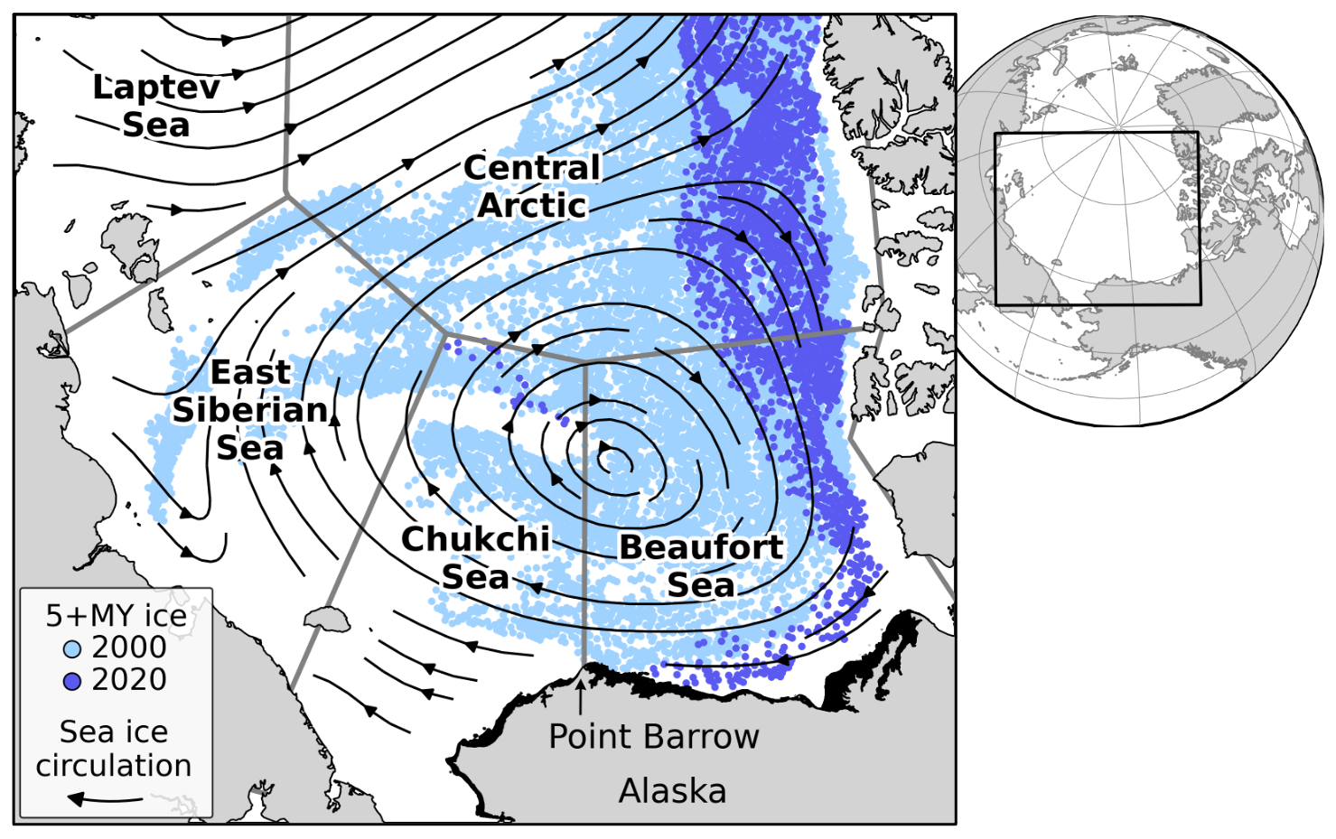
Figure 1 Coverage of ice older than 5 years from the week of 1 January during 2000 and 2020 from Tschudi et al. (2019b). Streamlines of mean January–April 2000–2020 Polar Pathfinder sea ice drift are overlain (Tschudi et al., 2019a). Ocean bathymetry of 20 m and shallower (GEBCO Bathymetric Compilation Group 2022, 2022) is filled in black around the Alaskan coast to demonstrate the typical regional landfast ice extent (Mahoney et al., 2007). Gray borders demarcate Arctic Ocean regions, as seen in Fetterer et al. (2010).

1.1 Climatological behavior of the Beaufort Gyre in winter

Sea ice motion is primarily driven by stresses from winds and ocean currents and modified by internal stresses from ice–ice interactions when sea ice concentrations exceed 80 % (Leppäranta, 2011). Winds describe the majority of sea ice motion away from coastal boundaries (Thorndike and Colony, 1982). Thus, the seasonal circulation structure of the Beaufort Gyre largely mirrors a pattern of anticyclonic surface winds that enclose a semi-permanent relative high in sea level pressure over the Beaufort and Chukchi seas – the Beaufort High (Walsh, 1978; Serreze and Barrett, 2011). The seasonal structure of the Beaufort High varies with the type, track, and persistence of synoptic weather systems that comprise it. The pressure fields of these atmospheric systems subsequently drive the variability in synoptic wind patterns that force the sea ice cover. Metrics such as the position of the Beaufort High (Regan et al., 2019; Mallett et al., 2021) or climate indices like the Arctic Oscillation (Rigor et al., 2002; Williams et al., 2016; Park et al., 2018) are often used to relate the variability in Arctic sea ice and ocean circulation to atmospheric forcing. For example, composite analyses of atmospheric and sea ice circulation have shown that in positive phases of the Arctic Oscillation, changes to the structure of the Beaufort Gyre circulation drive an anomalous ice thinning in the Pacific Arctic region (Rigor et al., 2002; Park et al., 2018). However, when assessed in individual years, these atmospheric metrics are only sometimes successful at describing dynamic ice conditions (Williams et al., 2016; Park et al., 2018). This suggests that other components of ice dynamics not captured by external forcing metrics play an important role in sea ice motion at seasonal to annual timescales.

Throughout late autumn and winter, sea ice concentrations increase, and the ice cover expands, meeting the nearly circumpolar Arctic coastline. During this period of sea ice consolidation, internal stresses from the interactions between the ice pack and the coast are readily transferred into the interior ice pack. The ice pack resists drift by redistributing stresses from external forcing that would otherwise force the ice into motion, thus causing internal ice stresses to build. Under this mechanism, internal stresses from ice–ice and ice–coast interactions modify ice kinematics, introducing spatiotemporal variability in the dynamic response of the ice to forcing from winds. As a result, correspondence between winds and ice drift weakens, especially when ice concentration is high (more than 80 %), and the high ice concentration is found within approximately 500 km of coastlines (Thorndike and Colony, 1982).

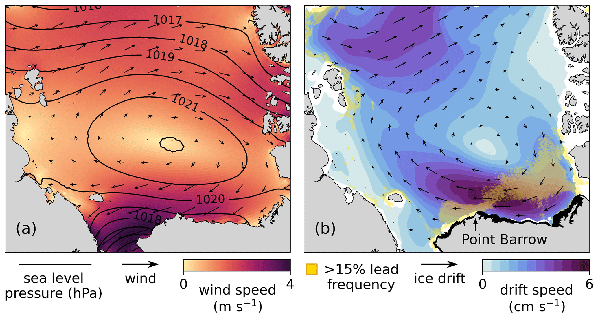
Figure 2 Climatological mean atmospheric and sea ice circulation fields (January–April 2000–2020). (a) ERA5 reanalysis with 10 m winds and mean sea level pressure contours. (b) Polar Pathfinder sea ice drift, overlain with MODIS-detected lead frequencies greater than 15 % for November–April 2002–2019 (Reiser et al., 2020). Alaskan landfast ice is shaded black, as in Fig. 1.

Most of the Beaufort Sea falls within the extent of considerable coastal constraint on ice motion. Incidentally, pressure gradients (i.e., winds) between the coast and the typical Beaufort High center describe less than half of the variance in ice flux across the sea (Howell et al., 2016). Between the months of January and April, the average Beaufort High and Beaufort Gyre patterns are centered in the northern Beaufort Sea (Fig. 2). We define January through April as the consolidated ice season in the Beaufort Sea, since these months typically follow the thermodynamic and dynamic consolidation of the ice cover in early winter and precede the breakup of the ice pack in spring. During this consolidated period, the Beaufort ice pack remains mostly contiguous with the Alaskan coast to its south and Canadian Archipelago to its east. More technically, the ice pack meets the landfast ice edge, which typically parallels the 20 m isobath along the Alaskan coast (Mahoney et al., 2007), and acts as a modified boundary condition on ice motion. Increased ice–ice and ice–coast interactions throughout the consolidated ice season produce large and highly variable internal stresses in the Beaufort Sea that constrain the flow of the Beaufort Gyre, complicating predictions of ice drift from winds alone.

1.2 Transient lead events

During the consolidated ice season, the winds of passing weather systems drive interactions between the Beaufort ice pack and the coast, increasing internal sea ice stresses. When local stresses exceed the strength of the ice, the ice cover fractures, producing discontinuities in the sea ice velocity field. These discontinuities often take the form of linear kinematic features, which can form leads if they open. The Beaufort Sea is a hotspot for leads, which are present for more than 15 % of winter days throughout much of the pack interior (Fig. 2b) and even more frequently at locations along the landfast ice edge (Willmes and Heinemann, 2015). Multiple headlands and sharp corners in landfast ice along the Alaskan coast act as stress concentrators, which initiate the formation of large-scale lead patterns that in some cases extend across the entire sea. This activity causes ice motion to transition intermittently between periods of relative quiescence and rapid drift on the order of hours, in association with large changes in internal stresses (Richter-Menge et al., 2002). These ice deformation events occur repeatedly throughout winter, making the nature of the Beaufort Sea ice velocity field challenging to predict and represent in models. Incorrect representations of transient internal ice stresses in association with recurrent deformation events could contribute to the particularly poor representation of consolidated Beaufort ice dynamics across a range of sea ice models (Kwok et al., 2008) – even relative to generally unrealistic climate model simulations of winter ice drift throughout much of the Arctic (Rampal et al., 2011; Tandon et al., 2018).

Recurrent patterns of lead opening from the landfast ice edge and promontories along the Alaskan coast have previously been visually identified and categorized based on their location and geometric characteristics (Eicken et al., 2005; Lewis and Hutchings, 2019). The main seaward coastal boundary prominence along the north Alaskan coast, Point Barrow, is a site of especially frequent lead activity (Willmes and Heinemann, 2015). A variety of lead patterns are initiated from the landfast ice around Point Barrow. Small-scale arches often extend westward from Point Barrow to Hanna Shoal (a shallow region ∼ 150 km offshore). Flaw leads open southeastward along the semi-stable landfast ice edge paralleling the Alaskan coast. Other patterns, those which will be the focus of this analysis, extend offshore into the central Beaufort and Chukchi ice packs. Previous observational analyses indicated that the locations of lead opening along the coast and associated patterns of ice flux throughout the Pacific Arctic region may be related to the position and persistence of weather systems traversing the region. These studies highlighted a need for further investigation into the connections between weather systems and changes in sea ice circulation that accompany specific patterns of coastal lead opening during the consolidated season. As sea ice models progress toward realistic representations of spatiotemporally discontinuous sea ice motion associated with coastal lead opening in the consolidated ice cover (e.g., Rheinlænder et al., 2022), observational descriptions of the relationships between winds, ice drift, and lead opening are needed to quantitatively evaluate the performance of model simulations.

1.3 Purpose of this study

The objectives of this study are to (1) acquire a deeper understanding of sea ice circulation in the Pacific Arctic region, given that coastal leads open from Point Barrow during the consolidated ice season, and (2) identify the weather patterns that initiate these recurrent events. We consider lead formation from 2000 to 2020 between January through April, since these months fall within the consolidated ice season. Within this time period, we explore the role that coastal geometry plays in constraining ice motion during lead-opening events, thereby providing insight into the broader role of ice–coast interactions in ice dynamics throughout winter and early spring. In particular, we evaluate these events relative to local climatology to discern spatial differences in ice drift as they arise from winds in the vicinity of the Alaskan coast.

This paper is organized as follows. In Sect. 2, we describe the methods used to identify Point Barrow lead-opening events and observationally characterize the dynamic conditions associated with them. In Sect. 3, we present the results of the analysis, including the range of synoptic atmospheric conditions associated with lead opening at Point Barrow, atmospheric and sea ice drift changes during an ensemble average lead-opening sequence, and controls on lead orientation and sea ice motion by patterns of wind forcing relative to the coast. In Sect. 4, we discuss connections between wind forcing patterns and coastal boundaries during opening events and the challenges in interpreting the impacts of an ensemble opening sequence due to variability across events. Finally, in Sect. 5, we summarize our results and their potential for guiding the development of sea ice models that aim to accurately represent the drift of the consolidated sea ice cover during these recurrent fracturing events.

2 Data and methods

2.1 Data from satellite imagery

Leads were identified with the Moderate Resolution Imaging Spectroradiometer (MODIS) Level-1B Calibrated Radiances in the longwave infrared band (band 31 from 10.780 to 11.280 µm). The longwave infrared band is useful for detecting leads due to the thermal contrast between the open water or thin ice within a lead and the thicker ice that surrounds it. Under favorable atmospheric conditions and with low viewing angle, a satellite's thermal imaging sensor may detect leads narrower than its resolution (Stone and Key, 1993). Lead widths as small as 200 m may be detectable with the 1 km resolution of MODIS band 31 under ideal conditions (Stone and Key, 1993). Cloud cover can increase the minimum resolvable lead width or even mask surface conditions altogether, preventing lead detection.

MODIS instruments are on board the Terra (EOS AM-1) and Aqua (EOS PM-1) satellites of the NASA Earth Observing System (EOS) program (MODIS Characterization Support Team (MCST), 2017a, b, c, d). Together, the satellites pass over the Beaufort and Chukchi seas approximately every 8 h. We acquired twice-daily (median times at 06:00 and 22:00Z) composite images of the study region, beginning in February 2000 after Terra's launch. Aqua's launch in spring 2002 provided an additional overpass (median at 13:00Z), increasing the collection to three times daily until the end of the analysis period in 2020.

2.2 Atmospheric reanalysis data

We used ERA5 atmospheric reanalysis (Hersbach et al., 2018) from the ECMWF to analyze atmospheric conditions. ERA5 has 0.25^∘ spatial resolution and hourly temporal resolution. We used hourly mean sea level pressure (SLP) and 10 m wind data for the months of January through April from 2000 to 2020. Daily averages were calculated from the hourly data. In an intercomparison of six atmospheric reanalyses against independent in situ observations, ERA5 most accurately reproduced observed 10 m wind speeds over Arctic sea ice in winter and spring (Graham et al., 2019), with a root mean square error (RMSE) of 1.4 m s⁻¹ from January–March and 1.1 m s⁻¹ in April–May.

2.3 Sea ice drift data

Sea ice velocity was taken from the Polar Pathfinder Daily 25 km EASE-Grid Sea Ice Motion Vectors data product (Tschudi et al., 2019a). The Polar Pathfinder drift product is generated using an optimal interpolation of remotely sensed sea ice drift data calculated from passive microwave sensors (AMSR-E, SMMR, SSM/I, and SSMIS), in situ drift data from buoys in the International Arctic Buoy Programme (IABP), and drift estimated from the National Centers for Environmental Prediction and the National Center for Atmospheric Research (NCEP–NCAR) Reanalysis 10 m winds. In an intercomparison of four sea ice drift products, the Polar Pathfinder product was shown to have the highest correlation with buoy drift data and a RMSE of 1 cm s⁻¹ in winter (Sumata et al., 2014).

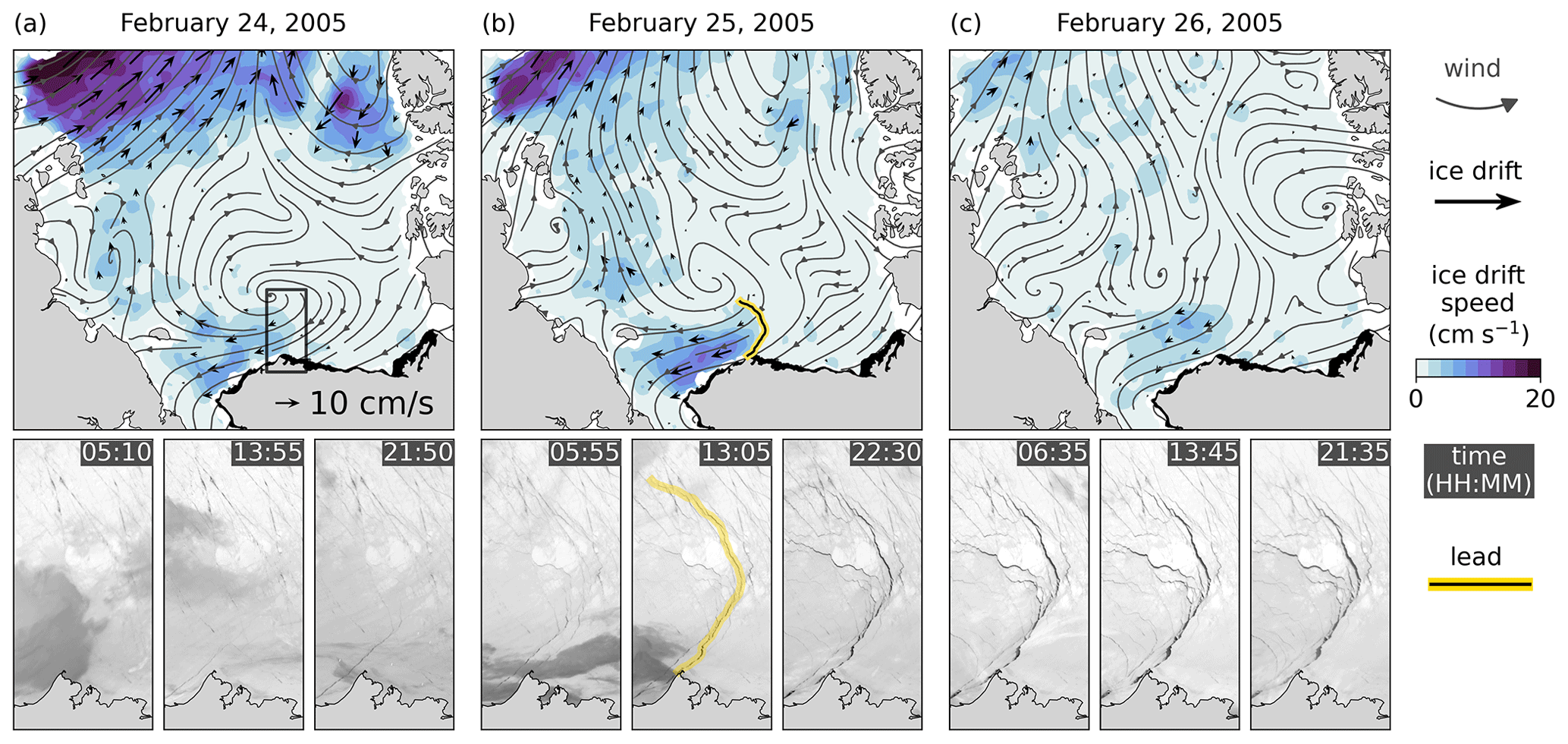
Figure 3 Lead identification and associated daily conditions from a lead event in winter 2005. The day of lead opening (DLO) is identified as 25 February. Top row shows the daily wind streamlines and sea ice drift. Bottom row shows the three daily thermal infrared MODIS images within the region that is outlined in the top row of panel (a). The image times are listed in UTC. Conditions are shown for (a) DLO−1, (b) DLO, and (c) DLO+1. The lead identified in the image from 13:05 UTC on the DLO is highlighted yellow and overlain in the top row of panel (b) (width not to scale). Alaskan landfast ice is shaded black in the top row, as in Fig. 1.

2.4 Lead identification and extraction from MODIS imagery

Leads were visually identified from three daily MODIS images over the analysis period. In images with limited cloud cover, the kinematic sea ice conditions were categorized, and the image was visually inspected for lead activity (Appendix A). Though cloud cover is at a minimum during winter and early spring (Intrieri et al., 2002; Shupe et al., 2011), the cloud cover was too extensive in 53 % of the analyzed images to determine lead presence at Point Barrow. An acceptable lead event was recorded if it met the following criteria: (1) low cloudiness, so as not to obscure the visual outline of a lead; and (2) neither a lead nor obscuring clouds was detected in the image before, so as to confirm no pre-existing lead.

Since the mechanisms of wind-driven lead opening are the focus of this study, constraints on the geometric characteristics of leads were used to omit certain lead patterns that form with considerable influence from factors other than winds. For example, the formation of lead patterns such as flaw leads or small-scale arches extending westward toward Hanna Shoal are strongly related to geographic and bathymetric features other than Point Barrow. To omit these patterns from consideration, leads were only included if they formed cohesive patterns extending northward from the landfast ice near Point Barrow into the offshore pack ice. An additional constraint was imposed in an effort to reduce the influence of ice heterogeneities on the formation of analyzed lead openings. Multiple leads will often form at Point Barrow in rapid succession, either as distinct lead patterns or as a system of leads branching from the same initial fracture as it deforms. This activity can influence the subsequent opening, since the deformation modulates the local thickness distribution and mechanical properties of the ice. Since the ice cover is continually deforming, impacts of such heterogeneities cannot be completely eliminated from this analysis. Hence, to reduce their influence on analyzed patterns, only leads that opened along a distinct path offshore from any other existing opening leads at Point Barrow were included in the analysis. In the case that a system of branching leads had formed between successive images, the bounding branch of the lead system (e.g., easternmost lead in a system of leads advancing eastward) was collected. In total, 135 leads satisfying these geometric constraints were identified. The lead identification process is demonstrated in Fig. 3, which shows three daily MODIS images in comparison to daily winds and ice drift associated with a lead identified on 25 February 2005.

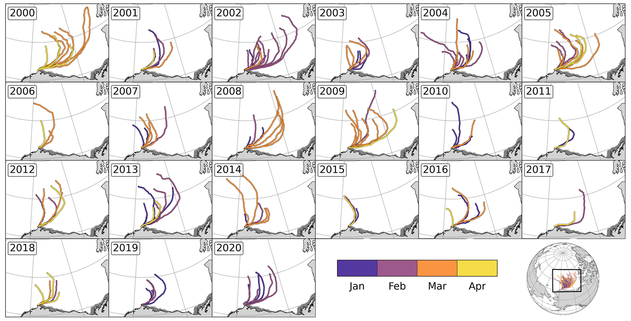
Figure 4 Leads identified in each year of the analysis. The lead color indicates the month in which the lead formed, namely January, February, March, or April. Lead widths not shown to scale. Alaskan landfast ice is shaded gray, as per Fig. 1.

Once the leads were identified, we used an active contour model (van der Walt et al., 2014) to semi-automatically extract lead coordinates from thermal MODIS imagery for each event (Jewell, 2023). Active contour models use iterative spline fitting to search for the strongest data contours through a set of given coordinates. These models are useful for the extraction of lead coordinates from thermal infrared imagery, in which relatively warm leads manifest as contrasting lines against the colder sea ice cover. Supplied with a number of manually selected imagery coordinates along each lead pattern from its connection to the landfast ice near Point Barrow to its terminus, the active contour model extracted the remaining coordinates, which were recorded with 5 km geodesic spacing (Fig. 3). Extracted lead coordinates for all 135 patterns are shown in Fig. 4. The MODIS images from which leads were extracted were mapped using a polar stereographic projection (central longitude 145^∘ W; extent 68.5–78^∘ N, 125–165^∘ W). The northernmost or westernmost coordinates of some lead patterns which extended outside of the study region were omitted.

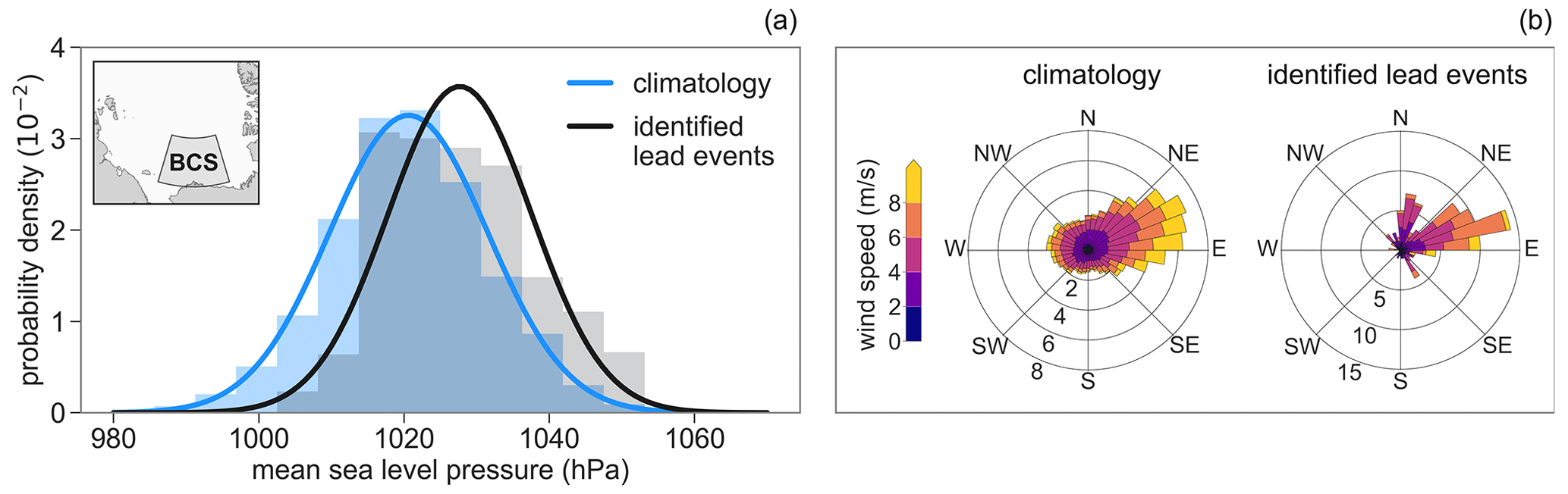
Figure 5 Distributions of atmospheric conditions during lead opening compared to climatology. (a) Distribution of mean SLP in the BCS region (inset map) across the 9 h windows preceding identified lead events and across the climatology (all hours for January–April 2000–2020). (b) Wind roses showing the distribution of wind speed and direction (from which the wind blows) for the mean wind vector of the BCS region, across the climatology and lead events. Radial labels indicate the percentage of wind directions that fall in each sector. Colors indicate the wind speed distribution within each sector.

2.5 Determination of atmospheric conditions during lead opening

The temporal window and spatial extent over which atmospheric forcing is relevant to lead formation at Point Barrow may vary across events. To characterize the relevant atmospheric conditions, we first considered a region over the Beaufort and Chukchi seas (BCS) between 70.5–78^∘ latitude and 187–220^∘ longitude (see Fig. 5). The BCS region is centered zonally around Point Barrow and extends meridionally from where the ice pack contacts the coast near Point Barrow to the center of the climatological (January–April 2000–2020) mean position of the Beaufort High. SLP and 10 m winds were spatially averaged in this region around the time of each lead formation. The time of lead formation cannot be precisely ascertained from the analyzed imagery for two primary reasons. First, a variable time lag follows each sea ice failure as it widens sufficiently to become visible in thermal MODIS imagery. For instance, a narrow shear failure may not become visible in satellite imagery until it is widened by winds (Overland et al., 1995). Second, a time lag separates the initial lead detectability and lead identification, since leads were identified from three daily images. In this analysis, each lead was assumed to have formed at some point between the image in which it was identified and the preceding clear-sky image. The average time gap between successive analyzed images is approximately 8 h. To determine the atmospheric conditions during the approximate time of lead opening, they were averaged over a 9 h period preceding and including the hour of the image in which each lead was collected.

2.6 Construction of an ensemble average lead formation event

We evaluated the typical dynamic conditions throughout the process of lead formation at Point Barrow by constructing an ensemble average sequence of daily atmospheric conditions, sea ice motion, and lead location across events. Identified events were aligned in time by the day of lead opening (DLO), with cross-event average atmospheric and sea ice conditions calculated from 3 d before to 2 d after the DLO. This 6 d period was chosen due to the similarity in synoptic atmospheric conditions across individual events within this window (Appendix B1). Many event sequences overlap, since multiple leads will often form in response to the same weather system. To eliminate the overlap across event sequences, sequences were only included in the ensemble if they did not overlap with any of the earlier included 6 d sequences. This reduced the ensemble size to 82 distinct lead-opening sequences, though the results are qualitatively similar when all 135 events are included in the ensemble.

For each day of the ensemble event sequence, daily SLP and sea ice drift anomalies were calculated relative to the climatological mean conditions (from daily mean conditions in January–April 2000–2020). Daily ice drift vector anomalies (${\mathit{u}}_i^{\prime }$) were calculated by subtracting climatological vectors (U_i) from the daily ensemble event vectors (u_i), as ${\mathit{u}}_i^{\prime }={\mathit{u}}_i-{\mathit{U}}_i$. Daily mean event wind speeds (${\stackrel{\mathrm{‾}}{u}}_{\mathrm{a}}$) and ice drift speeds (${\stackrel{\mathrm{‾}}{u}}_{\mathrm{i}}$) were also calculated across events for the ensemble. Climatological mean wind speeds (${\stackrel{\mathrm{‾}}{U}}_{\mathrm{a}}$) and ice drift speeds (${\stackrel{\mathrm{‾}}{U}}_{\mathrm{i}}$) were calculated for comparison. For portions of the analysis in which wind speeds were directly spatially compared to sea ice drift speeds, wind data were linearly interpolated to the 25 km EASE grid on which the Polar Pathfinder sea ice drift data are gridded.

To determine how the atmospheric conditions and sea ice circulation in the ensemble relate to the location of lead opening, the zonal mean lead position was calculated as a function of latitude across the 82 lead patterns from non-overlapping events. Because leads vary in length and orientation as they extend offshore, the mean and standard deviation in the zonal lead position become increasingly variable with increasing latitude (Appendix B2). The ensemble lead was therefore only calculated up to the latitude to which 70 % of the leads extend.

3 Results

3.1 Atmospheric conditions during lead opening

A unique signature is found in the synoptic atmospheric conditions over the BCS region in the hours during lead opening at Point Barrow. Figure 5 shows the wind and SLP distributions during opening of the 135 identified lead patterns. The distributions show that Point Barrow lead formation is associated with two primary wind directions (in contrast with the climatological wind distribution) and higher-than-average SLP over the BCS region, even relative to a high-pressure bias in cloud-free imagery.

The climatological (January–April 2000–2020) distribution of SLP in the BCS region is centered around 1020.6 ± 10.9 hPa. Across the 9 h windows associated with formation of the 135 identified lead patterns, the mean SLP increases to 1027.7 ± 9.9 hPa. This represents a statistically significant increase in mean SLP from climatology (t test; p < 0.01). Half of the pressure increase from the climatological mean may be attributable to a high-pressure bias introduced from the low-cloud requirement for lead identification (Appendix C). However, the other half constitutes an increase in the pressure distribution relative to both the climatology and the low-cloud imagery. It also co-occurs with a reduction in pressure variability relative to climatology and low-cloud imagery. This indicates that lead formation is usually associated with higher-than-average SLP over the BCS region.

Winds usually blow from the east-northeast over the BCS region (Fig. 5b), due to the climatological position of the Beaufort High (Fig. 2). In the climatological distribution, winds originating from the eastern quadrant are the most common (occurring 42 % of the time). Northerly (23 %) and westerly (21 %) winds are the next most frequent, and southerly winds (14 %) are relatively uncommon. During lead events, the distribution of wind direction diverges from the climatology. Winds during lead-opening events are primarily described by two distinct peaks from the east-northeast and north directions. Consequently, winds blowing from the east (54 %) and north (30 %) are more common during lead formation than in the climatology. Southerly (11 %) and westerly (5 %) winds are less frequent. Westerly winds are 4 times less frequent during lead-opening events relative to climatology. Thus, although westerly winds are relatively common in the region, they rarely initiate lead opening at Point Barrow.

The requirement for low-cloud cover does not bias the sampling of the wind direction associated with lead opening. This is evidenced by the similar wind distribution between climatology and low-cloud imagery (Appendix C). The frequencies of winds blowing from each cardinal quadrant in the cloud-free images are within 5 % of the climatological occurrences. Thus, we found little to no bias in wind direction associated with the lead detection methodology itself. In contrast to the large changes in wind direction between climatology and the identified lead events, wind speed in the BCS region varies little between the climatology (median 4.8 m s⁻¹), low-cloud images (median 4.5 m s⁻¹), and lead events (median 4.6 m s⁻¹).

3.2 Typical atmospheric and sea ice circulation during lead opening at Point Barrow

3.2.1 Ensemble average lead-opening sequence

In the ensemble average event, a high-pressure weather system travels northeastward across the Pacific Arctic region, driving lead opening from Point Barrow and producing asymmetric ice drift between the Beaufort and Chukchi seas. Figure 6 shows the sequence of atmospheric conditions and sea ice drift in the days before, during, and after the DLO in this ensemble lead-opening event.

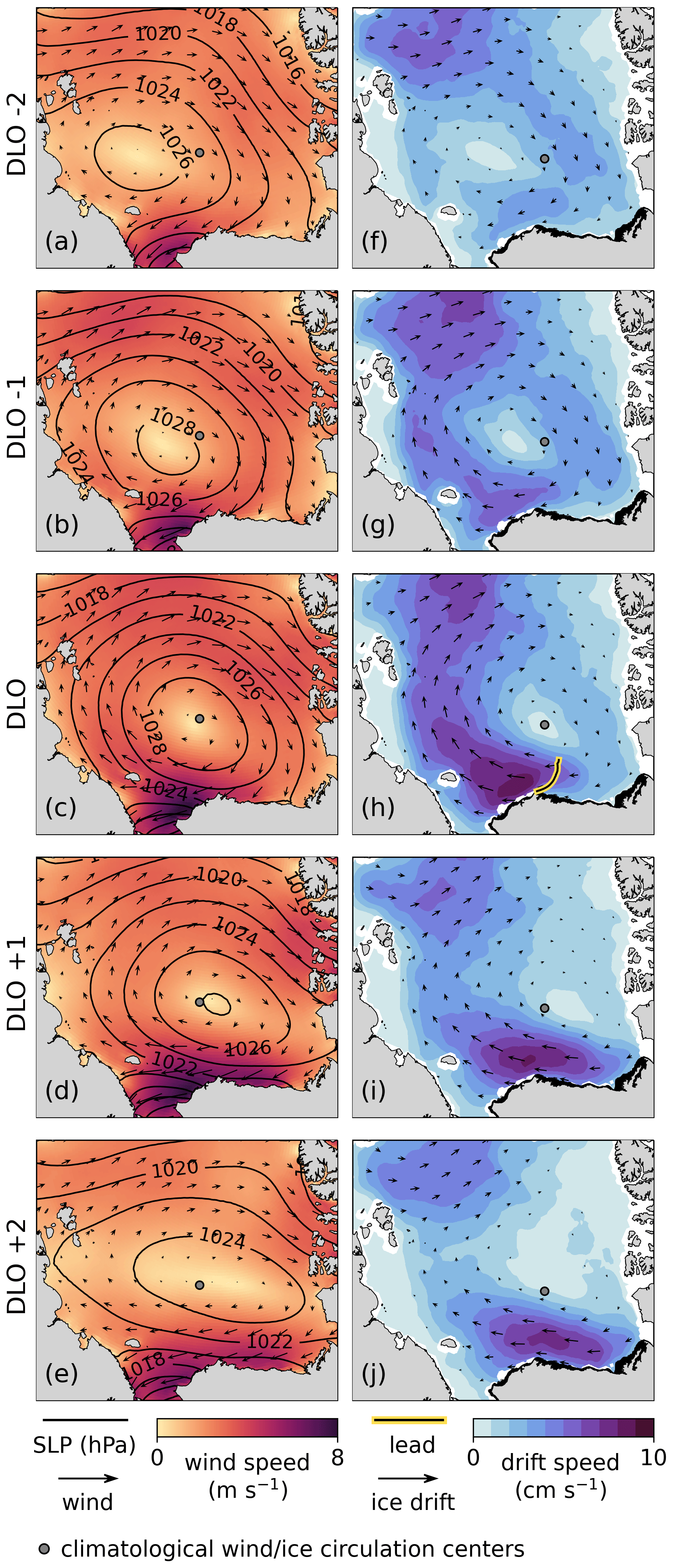
Figure 6 Ensemble lead-opening sequence. Mean atmospheric conditions (a–e) and sea ice circulation (f–j) over 5 d of the ensemble lead-opening event, centered around the DLO. The mean lead (yellow highlighted line in panel h; width not shown to scale) is displayed only on DLO, although individual openings can persist for longer. Alaskan landfast ice is shaded black, as in Fig. 1.

In the days preceding lead opening, a high-pressure atmospheric system travels northeastward from the East Siberian Sea towards the Beaufort Sea, strengthening winds from west to east along the Alaskan coast. The anticyclonic wind pattern and resultant anticyclonic sea ice circulation resemble the Beaufort High and Beaufort Gyre circulations, respectively, but both patterns are offset westward from their average January–April positions. Over the Beaufort Sea, northerly winds meet the Alaskan coast at a high angle, moving ice southward toward the coast. Restricted by the Alaskan coastal boundary, the Beaufort ice pack drifts southward slowly at speeds below 4 cm s⁻¹. In the Chukchi Sea, northeasterly winds strengthen and rotate clockwise over time, moving ice along and away from adjacent coastlines. In response, the ice cover accelerates and begins to drift northwestward around the ice gyre.

On the DLO, the ensemble average high pressure resides over the northern Chukchi Sea and reaches its maximum pressure. The centers of the wind and ice circulation patterns are co-located with their climatological positions on this day, but the shapes and strengths of the circulation patterns differ from the climatological patterns. Under sustained northerly wind forcing over the Beaufort Sea and strengthening easterly winds over the Chukchi Sea, the ice pack opens from the landfast ice edge near Point Barrow as a lead extends northeastward into the ice pack between the Beaufort and Chukchi seas. Ice drift speeds accelerate downwind of the fracture where the ice pack loses contact with the coast, while the upwind drift speed remains weak. As a result, a strong zonal gradient in the sea ice drift speed develops in the region between the high-pressure weather center and the Alaskan coast.

In the days following lead opening, winds shift easterly over the Beaufort ice pack as the high-pressure system continues traveling eastward. The winds also strengthen as they rotate, as is common in the Beaufort Sea, where easterly winds blow stronger than winds from other directions (Jewell and Hutchings, 2023). The zonal drift speed gradient between the Beaufort and Chukchi seas reduces as the rapid westward ice drift previously contained downwind of the lead extends east toward the Canadian coast of the Beaufort Sea. Eastward progression of accelerated drift speeds is often associated with additional lead patterns opening stepwise eastward from other headlands along the Alaskan coast, a recurrent behavior that occurs as anticyclones transit the region (Eicken et al., 2005; Lewis and Hutchings, 2019). Before the DLO, some of the westward ice export from the Beaufort Sea was replenished by a southward flow of ice into the northern Beaufort Sea. During the DLO, the westward ice export rapidly increases, while the northern import weakens. Following the opening, the ice drift pattern loses a closed circulation structure altogether, as motion of the northeastern ice pack stalls and the ice motion regime transitions to an export-dominated flow of ice from the Beaufort Sea.

3.2.2 Cross-event changes in ice drift across the position of lead opening

To determine whether the spatial differences in sea ice drift from the ensemble event are also reflected across individual events, we calculate the distributions of wind speeds and sea ice drift speeds in two equal-area regions (2 × 10⁵ km²) in the Chukchi and Beaufort seas across the 82 distinct event sequences (Fig. 7). The regions are separated by the mean lead position, with the Chukchi (C) region typically positioned downwind of the mean lead and the Beaufort (B) region typically located upwind.

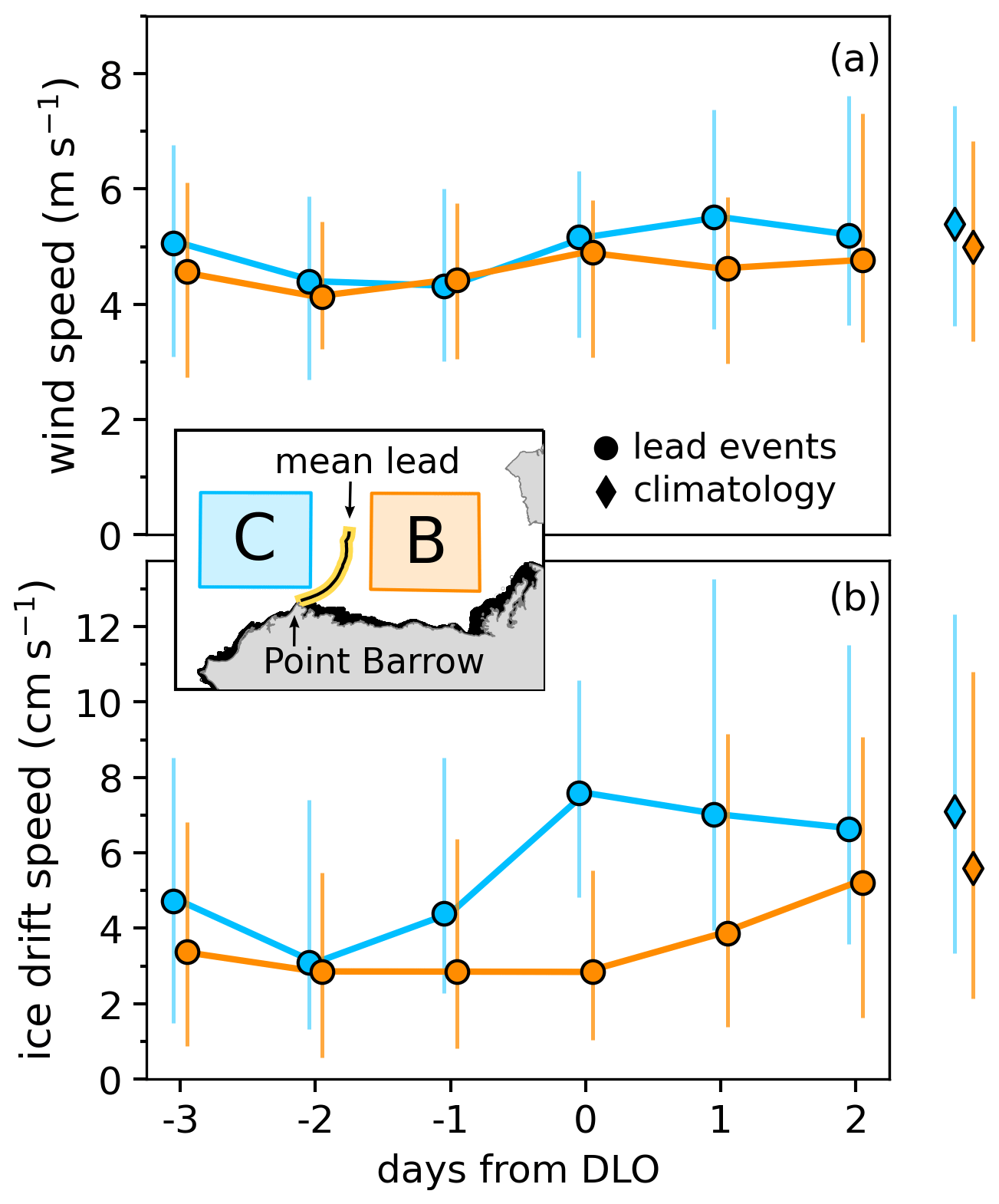
Figure 7 Comparison of the regional speeds across events. Distributions of the spatial average (a) wind and (b) ice drift speeds in regions C (blue) and B (orange). Regions are shown in an inset map. Alaskan landfast ice is shaded black, as in Fig. 1. Circles show the median across the 6 d of the 82 distinct time-aligned lead event sequences. Diamonds show the median across all days in January–April 2000–2020 (climatology). Vertical bars show the first and third speed quartiles.

Figure 7 shows the daily median wind and ice drift speeds in either region, which is calculated across event sequences aligned in time by the DLO. Results are qualitatively similar when calculated across all 135 events. The climatological daily speed distributions are also calculated in each region for comparison. The event distributions show that asymmetric ice drift in the vicinity of a lead at Point Barrow is seen not only in the ensemble event but also is reflected across individual events by differences in drift speed across the mean location of lead opening. Furthermore, they demonstrate that wind speed is remarkably similar between the two regions across events, and therefore differences in wind speed cannot explain the regional differences in ice motion.

In the climatological conditions, wind speeds in the Chukchi and Beaufort regions are similar, with Chukchi wind speeds on average 9 % faster than Beaufort wind speeds. The relative speed difference between the two regions is slightly greater for ice drift, with Chukchi sea ice drifting 20 % faster than ice in the Beaufort region on average. During lead events, wind speeds in the two regions remain similar, as they do in the climatology. From 3 d before the DLO until the DLO, the average wind speeds in the Chukchi region remain within 6 %–12 % of the average Beaufort wind speeds. During the 3 d before opening, the mean Chukchi drift speed across events remains within 24 %–36 % of the mean Beaufort drift speed. On the DLO, the regional ice drift speeds diverge considerably, despite maintaining similar wind speeds. Ice in the Chukchi region drifts at more than double the speed of ice in the Beaufort region. This greatly enhances the zonal asymmetry in ice drift along the Alaskan coast, while wind speeds remain zonally symmetric. Following lead opening, ice drift speeds in the Beaufort Sea begin to increase, while the Chukchi drift speeds decrease, reducing the drift speed asymmetry as the regional ice velocities return toward climatological conditions.

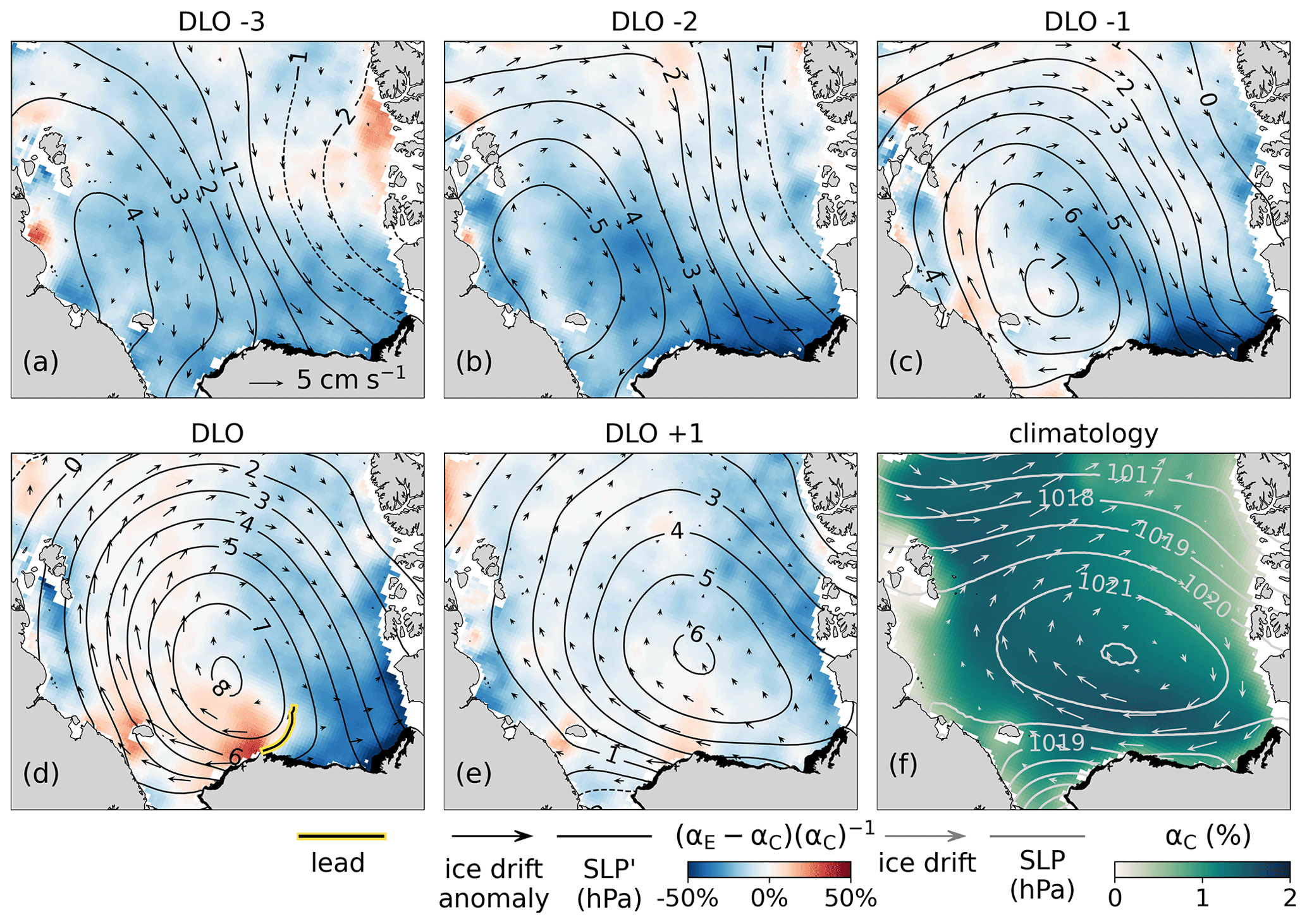
Figure 8 Ensemble sequence differences from climatology. (a–e) Relative difference in the ratio of ice drift to wind speeds between the event (α_E) and climatology (α_C) from DLO−3 to DLO+1. The figure is overlain with ice drift vector anomalies and SLP^′ contours. Solid (dashed) contours are positive (negative). The mean lead position is overlain on DLO in panel (d). (f) The ratio of climatological mean ice drift speeds to wind speeds is shown and overlain with climatological mean SLP contours and ice drift vectors. Alaskan landfast ice is shaded black, as in Fig. 1.

3.2.3 Anomalies in wind–ice relationships during the ensemble event

As demonstrated in Fig. 7, wind speeds do not explain the observed differences in sea ice drift speeds between the Beaufort and Chukchi seas during Point Barrow lead-opening events. Instead, as demonstrated in Fig. 5, wind direction appears to be the primary difference in wind forcing between climatology and the lead events. In Fig. 8, anomalies from climatology during the ensemble average event demonstrate how stronger-than-average zonal SLP gradients shift winds anomalously southward in the days preceding lead opening. The resultant differences in the patterns of wind forcing relative to the Beaufort and Chukchi coasts over time appear to impact the efficiency of the ice drift response to winds adjacent to these coastlines, explaining the zonal ice drift asymmetry associated with lead opening.

Figure 8f shows the ratio of the climatological mean ice drift speed to the climatological mean wind speed α_C = ${\stackrel{\mathrm{‾}}{U}}_{\mathrm{i}}{\stackrel{\mathrm{‾}}{U}}_{\mathrm{a}}^{-\mathrm{1}}$ throughout the Pacific Arctic region. This ratio is similar to the wind factor or Nansen number. However, rather than describing the instantaneous relationships between wind and ice drift, we calculate the ratio of the average wind and ice speeds at each location. Throughout much of the region, the ratio is near α_C ≈ 1.5 %. Near coasts and where winds push the thick multiyear ice cover of the central Arctic against the Canadian Archipelago, the ice is less responsive to wind forcing, and α_C is smaller. Under the predominantly meridional SLP gradient north of Point Barrow, α_C is slightly enhanced, compared to other regions, as ice drifts parallel to the coast. Under this prevailing forcing pattern, sea ice in the Beaufort and Chukchi seas appears to exhibit similar responsiveness to winds.

During the ensemble event, the spatial pattern of the ice–wind speed ratio deviates from the climatological pattern. The daily speed ratio for the event is calculated from the ensemble mean ice drift and wind speeds as α_E = ${\stackrel{\mathrm{‾}}{u}}_{\mathrm{i}}{\stackrel{\mathrm{‾}}{u}}_{\mathrm{a}}^{-\mathrm{1}}$. Figure 8a–e shows the relative difference in the ice–wind speed ratio during the event from the climatology between DLO−3 and DLO+1, which is calculated as $({\mathit{\alpha }}_{\mathrm{E}}-{\mathit{\alpha }}_{\mathrm{C}})({\mathit{\alpha }}_{\mathrm{C}}{)}^{-\mathrm{1}}$. Anomalies in SLP (SLP^′) and ice drift vector anomalies are also overlain. To reduce clutter, wind vector anomalies are not included in the figure. Their directions can be visually estimated from the SLP^′ contours, as they are typically rotated slightly counterclockwise from geostrophic alignment along SLP^′ contours.

In the days preceding lead opening (DLO−3 through DLO−1), a SLP^′ high resides over the East Siberian Sea that is offset southwest from the mean January–April Beaufort High position. The SLP^′ gradient is predominantly zonal across the Beaufort and Chukchi seas, producing southward ice drift anomalies that move ice toward the Alaskan coast. The ice drift anomalies align with local SLP^′ contours throughout most of the region, except in the southern Beaufort Sea, where the consolidated ice pack is restricted by the rigid Alaska coastal boundary, and the ice drift vector anomalies are deflected eastward along the coast. The ice is less responsive than usual to wind forcing throughout most of the Pacific Arctic region under this synoptic forcing pattern, particularly in the southern Beaufort Sea, where ice drifts 40 % slower relative to winds than in the climatology.

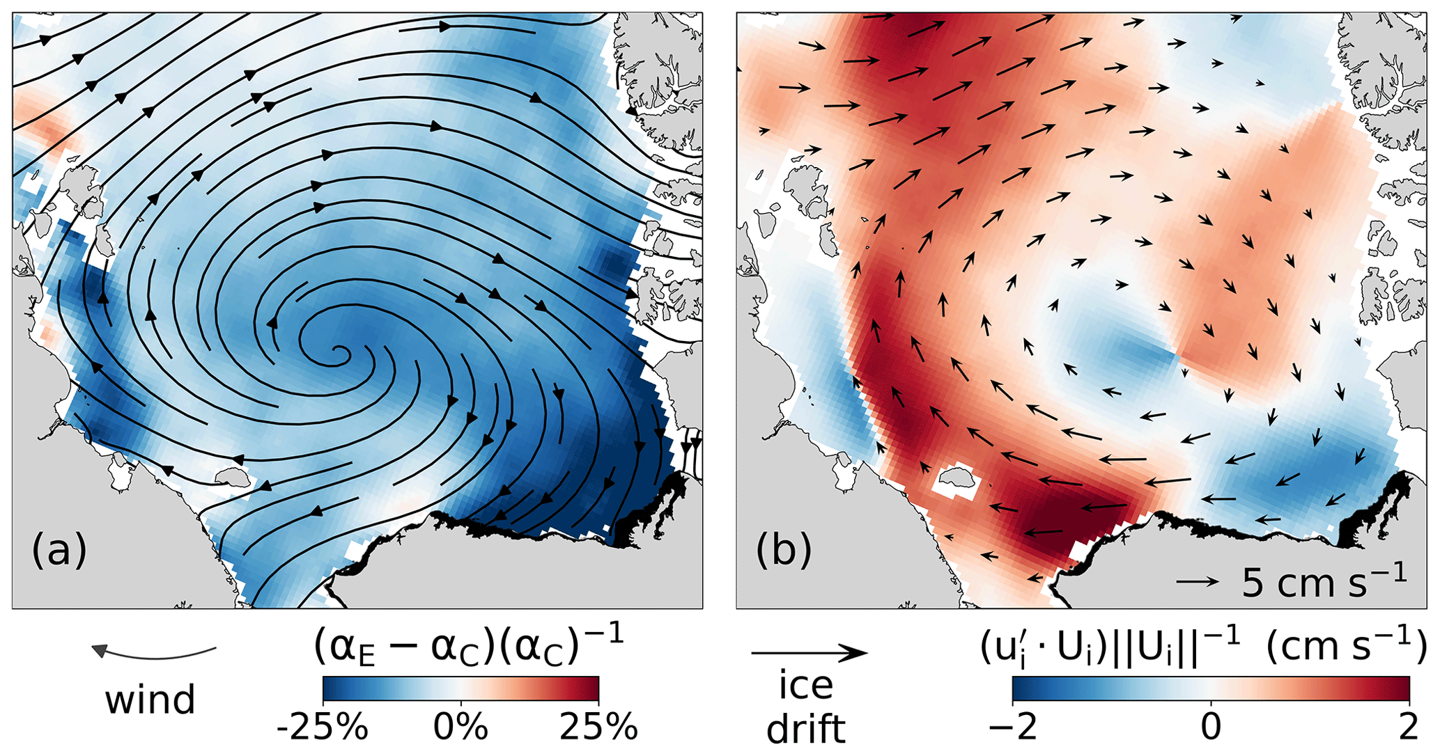
Figure 9 Zonal asymmetries in ice–wind relationships and contributions to climatological ice drift. (a) Relative difference from climatology in the ice-to-wind speed ratio averaged over the 6 d ensemble sequence. Streamlines of average winds are overlain. (b) Component of the average 6 d ensemble ice drift anomaly along the climatological ice drift, which is overlain with 6 d average ice drift vectors. Alaskan landfast ice is shaded black, as in Fig. 1.

Between DLO−3 and DLO, the SLP^′ high migrates eastward. By the DLO, zonal gradients in SLP^′ still dominate throughout the region. However, because the SLP^′ high is positioned slightly west of Point Barrow, the pattern of anomalous synoptic forcing meets the Chukchi and Beaufort coasts of Alaska differently. East of the SLP^′ high, a zonal pressure gradient anomaly persists in the Beaufort Sea and continues to drive northerly wind anomalies which force the ice pack against the coast. An anomalously weak ratio of ice drift to wind speeds remains in the Beaufort Sea. In contrast, a positive anomaly in the ratio of ice drift to wind speeds develops in the Chukchi and East Siberian seas, where gradients in SLP^′ drive easterly and southerly wind anomalies, respectively. Under this drift-favorable wind pattern, ice drift in these regions becomes temporarily more responsive to winds than usual. Directly downwind of opening in the Chukchi Sea, ice drifts up to 40 % faster than usual relative to winds. The position of lead opening demarcates the regions of the ice pack experiencing enhanced and weakened responsiveness to wind forcing. This approximately parallels the SLP^′ contour that meets Point Barrow, which separates the anomalous against-coast forcing over the Beaufort ice pack from the offshore forcing over the Chukchi Sea.

Following lead opening (DLO+1), the SLP^′ high travels further eastward and begins to weaken. A meridional SLP^′ gradient expands eastward across the Beaufort Sea, producing westward ice drift anomalies in both the Beaufort and Chukchi seas. As the directions of forcing align with or point offshore from the Alaskan coast in the two seas, the differences in ice drift responsiveness to winds between the two regions reduces. The synoptic loading pattern returns to the climatological norm, as does the ice–wind speed ratio.

3.2.4 Contribution of the ensemble lead sequence to climatological ice drift

Though leads open from Point Barrow in a matter of hours, the identified opening events tend to follow sequences of similar atmospheric conditions and ice motion spanning several days. Persistent reductions in Beaufort ice drift speeds relative to wind speeds upwind of where the lead patterns form result in spatially varying contributions to the climatological Beaufort Gyre circulation during these multiple-day lead event sequences. To demonstrate this, Fig. 9 shows atmospheric conditions and ice circulation averaged over the full 6 d ensemble lead sequence. Figure 9a shows the 6 d average SLP and winds overlain on the relative difference in the event ice-to-wind speed ratio from climatology calculated from the average wind and sea ice drift speeds across the 6 d sequence. Figure 9b shows the 6 d average ice circulation pattern. Underlain is the component of the 6 d average ice drift vector anomalies aligned along the climatological drift vectors, calculated as $({\mathit{u}}_i^{\prime }\cdot {\mathit{U}}_i)\left|\right|{\mathit{U}}_i|{|}^{-\mathrm{1}}$. This quantifies how the ensemble ice drift contributes to the climatological ice circulation over the 6 d sequence. Positive values show where the anomalies are aligned along the typical flow direction, corresponding to a strengthening of the climatological drift pattern during the events. Negative values represent vector anomalies aligned against the climatological vectors and a weakening of the climatological drift.

On average over the ensemble sequence, ice drifts slightly (0 %–10 %) slower than usual relative to wind speeds throughout most of the Pacific Arctic region (Fig. 9a). Wind streamlines (curves tangent to the local wind velocity) are displayed in Fig. 9a to trace the direction and extent of wind forcing across the region. North of Alaska, the wind streamline intersecting Point Barrow marks the transition between where the Beaufort and Chukchi ice packs are forced along or against the coast due to the change in the coastline orientation at Point Barrow. West of the streamline in the Chukchi Sea, the ice-to-wind speed ratio shows little appreciable difference from climatology over this 6 d period, as the average winds move ice along the coast. Thus, the enhancement in ice drift speeds that occurs downwind of the lead patterns on the day of opening (Fig. 8d) is offset by weaker ice drift preceding opening, and the signal of lead-associated ice acceleration is lost over this longer period. In the Beaufort Sea, east of the wind streamline intersecting Point Barrow, a clear ice-to-wind speed ratio anomaly remains over the 6 d sequence. Persistent onshore wind forcing over this period moves ice against the Alaskan coastline east of Point Barrow preceding and during opening, reducing the ice-to-wind speed ratio by more than 25 % below climatology over the full sequence.

As a result of these varying wind-driven ice–coast interactions, the ensemble lead-opening sequence's contribution to the climatological Beaufort Gyre circulation varies regionally. Figure 9b demonstrates this, showing a pronounced zonal asymmetry in gyre strength along the Alaskan coast during the ensemble sequence. The western flow of the Beaufort Gyre is strengthened by 1–2 cm s⁻¹ on average throughout the ensemble, strengthening ice advection across the Chukchi, East Siberian, and Laptev seas, where winds move ice along or away from the coasts. Strengthening is greatest along the Chukchi coast of Alaska, where the climatological drift is enhanced by over 2 cm s⁻¹. The change in coastline orientation at Point Barrow marks the transition between the western strengthening and simultaneous eastern weakening of climatological winter ice transport. To the east in the Beaufort Sea, the gyre is weakened by up to ∼ 1 cm s⁻¹ during the ensemble sequence. The differences in ice-to-wind speed ratios between these regions shown in Fig. 9a suggests that differing mechanisms underlie the contrasting contributions to the climatological drift. In the seas west of Point Barrow, relatively small anomalies in the ice–wind speed ratios from average winter conditions indicate that the strengthening of the climatological drift over the ensemble sequence does not result from substantial changes to the responsiveness of the ice to local winds. Rather, the strengthened ice circulation in the western regions results from a typical ice drift response to a strengthening of the climatological wind pattern (not shown). In the Beaufort Sea, however, the ice–wind speed ratio is much weaker than normal winter conditions. There, onshore wind anomalies persist throughout much of the event sequence, increasing ice interaction with the coast during the events. A resultant reduction in the typical winter ice responsiveness to winds produces the weakened ice circulation east of Point Barrow.

3.3 Controls on ice drift and location of opening by wind direction

The ensemble lead-opening sequence shows how the migration of a high-pressure weather system on average initiates lead opening at Point Barrow. Across individual events, the positions and structures of high-pressure systems vary, including on the days when leads open. These variable SLP patterns produce a range of wind forcing conditions over the BCS. Each wind pattern drives lead formation at Point Barrow but does so by initiating different patterns of regional ice drift and orientations of lead extension into the Beaufort ice pack.

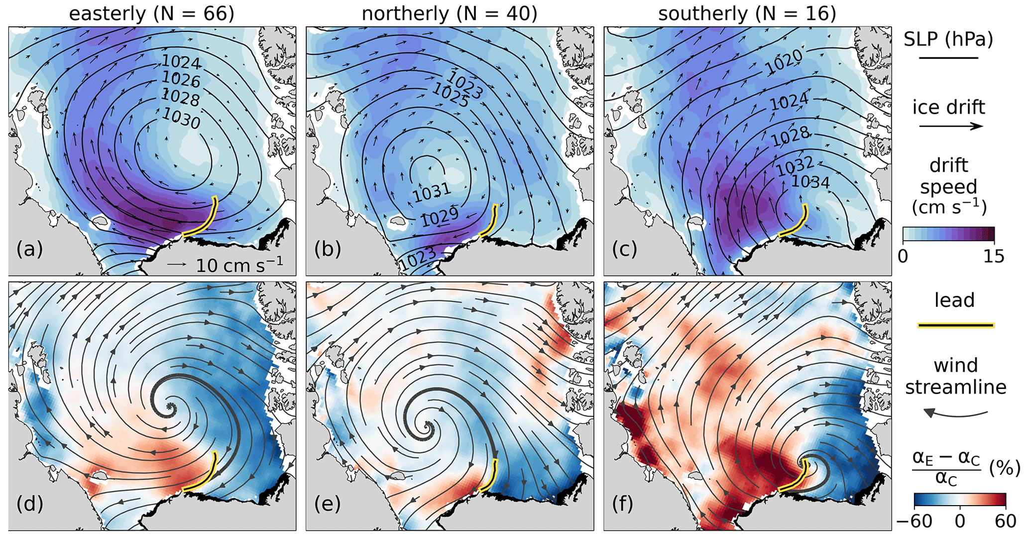
Figure 10 Lead ensembles sorted by BCS wind direction, including easterly (a, d), northerly (b, e), and southerly (c, f) directions. The top row (a–c) shows the daily ice drift overlain with SLP contours for each ensemble. The bottom row (d–f) shows the relative differences in ice-to-wind speed ratios from climatology. Wind streamlines are overlain. The streamline intersecting Point Barrow is shown in bold. The mean lead position is overlain on both rows for each ensemble. Alaskan landfast ice is shaded black, as in Fig. 1.

To explore the range of wind forcing conditions that can initiate Point Barrow lead opening and their impacts on ice drift and lead formation, we separate events into three types, based on the direction of wind forcing over the BCS during the 9 h window in which leads were assumed to have formed (see the wind distribution in Fig. 5). Each type is defined by a cardinal direction quadrant, namely those that occur under northerly winds (originating from NW through NE), easterly winds (NE through SE), and southerly winds (SE through SW). Only six events occurred under westerly winds (SW through NW), comprising less than 5 % of the identified events. Due to their small sample size, westerly cases are omitted from this portion of the analysis. The distributions of their high-pressure centers and resultant lead patterns can be found in Fig. B2. For each of the three included categories, an ensemble average lead event is calculated on the DLO by averaging the daily atmospheric conditions, ice drift, and location of lead opening across individual events. The relative differences from climatology in ice–wind speed ratios are also calculated for each category. The ensemble average lead events are shown in Fig. 10.

3.3.1 Easterly winds

Lead opening at Point Barrow is most often driven by easterly winds over the BCS region. Easterly winds precede 71 events, corresponding to the largest peak in the Fig. 5 wind distribution. The ensemble average event is calculated across 66 distinct event days (since some events occur on the same day) and is shown in Fig. 10a. On average, this event type is associated with a high-pressure system located 800 km north of Point Barrow. The position and structure of this high determines the location of the wind streamline that intersects Point Barrow (overlain in Fig. 10d), which separates two regimes of forcing over the ice based on the wind direction relative to Alaska's Beaufort and Chukchi coastlines.

On the eastern side of the Point Barrow streamline, winds with an onshore component compress ice in the eastern Beaufort Sea against the Alaskan coast. As a result, northern ice import into the Beaufort Sea nearly stalls (drift speed < 2 cm s⁻¹), and ice to the south drifts slowly westward. On the western side of the streamline, winds direct the ice pack along and away from the Chukchi coast. Unrestrained by coastal boundaries, ice in the western Beaufort and Chukchi seas drifts rapidly (> 10 cm s⁻¹). This produces a large ice drift speed gradient across the Beaufort and Chukchi seas. A lead opens near the coast along the wind streamline intersecting Point Barrow. As the lead extends offshore, it turns against the local wind direction and curves toward the center of the high-pressure system in a concave west arched pattern. Downwind of the lead, ice drifts faster than usual relative to local wind speeds, transporting ice towards the Transpolar Drift. Upwind of the lead, where the ice pack remains restrained by the coast, the ice drifts anomalously slowly relative to winds in comparison to climatological conditions.

3.3.2 Northerly winds

Northerly winds are the second most common driver of identified events. These winds precede 42 events and capture the second-largest wind direction peak in Fig. 5. The ensemble average conditions are calculated across 40 distinct event days, as shown in Fig. 10b. On average, this event type is associated with a high-pressure system located 750 km northwest of Point Barrow. Northerly winds dominate throughout the Beaufort and Chukchi seas. Thus, the wind streamline intersecting Point Barrow approaches the coast from further west than in the easterly wind ensemble. Consequently, a greater portion of the Beaufort Sea experiences onshore wind forcing relative to that of the easterly ensemble. Given the proximity of the high to adjacent coastlines in the Chukchi and East Siberian seas, a smaller region west of the streamline experiences the alongshore-wind forcing that is conducive to ice drift.

The average northerly lead pattern forms in alignment with the wind streamline intersecting Point Barrow along its entire calculated extent. The lead demarcates a rapid alongshore ice drift (reaching 10 cm s⁻¹) in the Chukchi Sea, where the ice-to-wind speed ratio is enhanced compared to climatology, and weak drift in the Beaufort Sea (below 3 cm s⁻¹), where the ice-to-wind speed ratio is reduced. In contrast to the easterly event type, the northerly event features both westward Beaufort Sea ice export in the south and import at the sea's northern boundary. The regional pattern of ice drift is characterized by a closed circulation offset westward from the climatological pattern.

3.3.3 Southerly winds

Southerly winds less frequently initiate lead opening at Point Barrow and only precede 16 of the identified events. On average, they are associated with a high-pressure system located 400 km northeast of Point Barrow (Fig. 10c). Given the proximity of the high to the coast, the wind streamline meeting Point Barrow approaches the coast from a low angle and over a short extent. Offshore winds dominate across much of the western Arctic, driving exceptionally strong ice drift relative to wind speeds downwind of the lead. Directly west of the lead, ice drifts more than 60 % faster relative to winds than in climatology. Ice east of the Point Barrow streamline drifts slowly with an anomalously low ice-to-wind speed ratio. In some locations, ice drifts more than 60 % slower relative to winds than usual, as winds pile ice into the southeastern corner of the Beaufort Sea, where both the east–west- and north–south-oriented coastlines mechanically impede ice drift.

The average lead opens at a low angle from the coast and terminates at the center of the average high-pressure system. This forms an arch-shaped lead pattern that opens perpendicular to the local direction of ice drift along most of its extent. Unlike the northerly and easterly cases, which feature complete or partial alignment of leads with local winds, the southerly lead does not align with the Point Barrow wind streamline, except at its connection to the coast. Instead, it opens west of the streamline, where winds move ice offshore from the Beaufort coast into the Chukchi Sea.

4 Discussion

Here we discuss implications of the observed processes during Point Barrow lead-opening events. First, we discuss the sensitivity of ice drift to local wind forcing during these events and how this may challenge predictions of ice dynamics from atmospheric metrics such as climate indices or pressure centers. Next, we consider differences in ice–wind relationships across Point Barrow during lead opening and how this may reflect internal ice stresses which depend on wind patterns and coastline geometry. Finally, we discuss the variability across events and how these lead-opening sequences contribute to the climatological Beaufort Gyre circulation.

4.1 Sensitivity of ice drift to synoptic wind forcing patterns

In this analysis, we demonstrate the sensitivity of sea ice motion to the structure of synoptic-scale wind patterns on timescales of days to a week. By doing so, we offer insight into mechanisms modulating ice drift that challenge predictions of sea ice circulation from metrics such as climate indices or the positions of synoptic atmospheric forcing patterns.

On the DLO in the ensemble average lead sequence, the center of the average wind circulation pattern is aligned with its climatological position (the center of the January–April mean Beaufort High). Though the ensemble pressure pattern aligns with the Beaufort High, it features a stronger zonal pressure gradient than that of the climatological pressure field. This results in wind direction anomalies over spatial scales on the order of 500 km. The resultant wind pattern drives an anticyclonic sea ice circulation that is aligned with its climatological position (the January–April Beaufort Gyre center) but deviates considerably from the mean gyre pattern. During the ensemble event, the smoothly varying velocity field of the climatological gyre's southern flow is disrupted by large-scale fracturing of the ice cover between the Beaufort and Chukchi seas. A strong zonal asymmetry in sea ice drift speeds develops between the two regions that is absent from the climatological mean flow, resulting in anomalous ice flux patterns across the Pacific Arctic region. These findings demonstrate how regional wind anomalies can limit predictability of large-scale ice motion. Even as the center of a synoptic forcing system (e.g., a passing high) aligns with a known center of action (e.g., the mean Beaufort high position), regional wind differences between the two aligned forcing systems can yield pronounced differences in the large-scale ice circulation.

Consideration of the variability across events provides additional insight. Across identified Point Barrow lead-opening events, winds over the BCS region typically originate from the north or east-northeast directions (Fig. 5) and are primarily associated with high-pressure atmospheric systems. However, the centers of the high-pressure weather systems that drive these winds are broadly distributed over the Arctic Ocean (Fig. B2). Thus, lead opening at Point Barrow can be driven by anticyclones positioned at a range of locations, so long as they produce the appropriate wind directions over the BCS region. This finding indicates that specific alignment of a synoptic forcing pattern is not always required to initiate recurrent dynamic ice behaviors.

Altogether, these observations indicate that the drift of the consolidated ice pack is highly sensitive to the patterns of synoptic atmospheric forcing relative to coastlines. Such sensitivity has also been demonstrated in a modeling study (Rheinlænder et al., 2022) in which a dynamic sea ice model was used to simulate a large-scale Alaska coastal sea ice fracturing event in the Beaufort Sea (corresponding to Point Barrow leads identified in this analysis on 20–21 February 2013). When forced with different realizations of the same weather system from multiple atmospheric reanalysis products, the relatively small differences in forcing produced large differences in the timing and location of coastal lead opening and the associated ice velocity fields. Thus, both observations and models suggest that in order to simulate the ice transport associated with these events, high accuracy in synoptic forcing fields is required.

4.2 The role of coastal interactions

As the ice pack consolidates against the coast in winter, stresses from ice–coast interactions are transmitted offshore, and underlying stress levels increase throughout the ice pack (Richter-Menge et al., 2002). Errors in the modeled drift of the consolidated coastal ice pack likely arise in part from inaccurate representations of this ice stress development and transmission. An improved representation of the modeled ice interactions requires an understanding of the large-scale stress fields that constrain ice motion in coastal regions. However, efforts to understand the nature of the internal stress field currently rely on sparse in situ stress measurements (Richter-Menge et al., 2002) or interpretations of modeled stress fields (Steele et al., 1997), which rely on ad hoc constitutive relationships between stress and ice kinematics.

Internal ice stresses cannot be directly resolved from the observational data employed in this analysis. However, stress states can be inferred using theoretical and measured connections between ice stress and kinematics. Linear relationships between winds and ice drift successfully describe the ice motion in summer when ice concentrations and internal stresses are low. As internal stresses increase during the consolidation of the ice pack in winter, the ratio of ice drift to wind speeds decreases, and the correlation between winds and ice drift weakens, especially near coastal boundaries (Thorndike and Colony, 1982). Reduced ice-to-wind speed ratios may therefore indicate increasing ice stresses that reduce the efficiency of wind-to-ice momentum transfer. Stress reduction may manifest as an increase in the ice-to-wind speed ratio. With this context, the findings in this analysis provide insight into the potential spatial extent over which the stress transmission from the Alaska coastal boundary modulates the response of the consolidated ice cover to different wind forcing patterns.

Point Barrow marks an abrupt transition between the southwest–northeast orientation of Alaska's Chukchi coast and the predominantly east–west orientation of its Beaufort coast. Contrasting ice–wind relationships adjacent to the coastal boundaries on either side of Point Barrow suggest that Alaska's coastal geometry exerts a dominant control on the development of spatiotemporally varying ice stresses that modulate consolidated ice dynamics. Preceding lead opening at Point Barrow, southward wind anomalies compress the Beaufort ice pack against the Alaskan coast. This results in anomalously low ice-to-wind speed ratios relative to typical winter conditions. This anomaly extends approximately 500 km offshore (Fig. 8), potentially reflecting the spatial extent of increased ice stresses under the ensemble wind forcing pattern. As the high migrates eastward, wind anomalies over the Chukchi ice pack rotate to direct ice motion away from the Chukchi coast, opening a lead between the Beaufort and Chukchi seas. The lead bounds positive anomalies in the local ice-to-wind speed ratio where the ice pack pulls away from the coast, signaling a reduction in internal ice stresses. These interpretations align with previous in situ measurements of stress in the consolidated winter ice pack. Richter-Menge et al. (2002) showed that large ice stresses can be detected more than 500 km from shore in the Beaufort Sea, as onshore winds compress the ice pack against the coast (Richter-Menge et al., 2002). When winds move ice away from coastal boundaries, stresses can fall to near-zero levels (Richter-Menge et al., 2002).

Across the northerly, easterly, and southerly wind ensembles, leads open along or west of the wind streamline intersecting Point Barrow (Fig. 10d–f). This wind streamline approaches the coast from different locations, thereby producing different lead orientations and separating out differing portions of the Beaufort and Chukchi ice packs that experience strengthened and weakened drift efficiency. These cases demonstrate the variable spatial extents of potential ice stress regimes, depending on the direction of wind forcing.

4.3 Interpreting impacts of Point Barrow lead-opening events

The Beaufort Gyre redistributes sea ice volume throughout the Arctic, thereby influencing regional susceptibility of sea ice to melt in summer. In recent decades, net sea ice export from the Beaufort Sea between January and April has been significantly negatively correlated with its sea ice area at the end of the following summer, suggesting a dynamic winter preconditioning of summer ice conditions (Babb et al., 2019). The episodic drift and deformation events that dominate Beaufort Sea ice motion during the consolidated ice season challenge predictions of dynamic sea ice change over seasonal timescales and longer.

Leads open from Point Barrow over a number of hours. However, this analysis shows that Point Barrow lead events are usually associated with the migration of an atmospheric high over several days. Cross-event SLP variability is reduced relative to climatological SLP variability from 3 d before to 2 d after lead opening. This offers some degree of predictability for the contribution of these events to seasonal ice motion. On average over this 6 d period, the pattern of ice circulation appears similar to the climatological Beaufort Gyre. However, the contribution to the gyre is zonally asymmetric across Point Barrow. The western flow of the gyre is enhanced, while the southeastern flow in the Beaufort Sea is weakened. Previous work has similarly shown that average winter ice flux is enhanced in the Chukchi Sea and weakened across the Beaufort Sea on days when large-scale lead patterns are present at Point Barrow (Lewis and Hutchings, 2019).

We identified 82 distinct event sequences in the form of nearly one 6 d sequence per month over the analysis period. Cumulatively, these events span approximately one-fifth of the winter periods (January–April) between 2000 and 2020. This is a conservative estimate, as nearly 40 % of the total 135 identified lead-opening events overlapped with the distinct sequences included in the ensemble. Given the frequency of these episodic events throughout the consolidated season, their associated ice drift patterns must be understood and represented accurately in models in order to support predictions of ice transport on seasonal timescales.

Across events, there is variability in the track, persistence, and structure of anticyclonic weather systems that initiate lead opening at Point Barrow. The days that leads open can be followed by a range of dynamic ice conditions. Some Point Barrow events are followed by a rapid return to quiescent conditions (e.g., Fig. 3). Other events are followed by steady ice export for a number of days following the initial opening, as is the case in the ensemble average sequence. Eastward migration of an anticyclone that increases the extent of easterly wind forcing over the Beaufort Sea can open additional leads from other headlands along the Alaskan coast (Jewell and Hutchings, 2023; Lewis and Hutchings, 2019). Under sufficient forcing, the entire Beaufort ice pack can separate from landfast ice along the Alaskan and Canadian coastlines, causing extensive fracturing and increased ice transport along the Alaskan coast. Point Barrow lead-opening events often precede such events but are not always followed by sustained ice transport. Thus, the conditions shown in the ensemble are not necessarily predictive of ice circulation changes during individual events, particularly following lead opening. Furthermore, cumulative sea ice transport can be overwritten by changes in sea ice dynamics over a relatively short period of time (Babb et al., 2019). Care should therefore be taken in predicting sustained impacts on the regional sea ice cover based on individual fracturing events.

5 Summary and conclusions

Point Barrow exemplifies Alaska's unique coastal geometry and is a trigger site for exceptionally high rates of lead opening in winter. This paper uses observational and reanalysis data to investigate changes in Pacific Arctic sea ice circulation as large-scale lead patterns open from Point Barrow. Low-cloud MODIS imagery was used to visually identify 135 Point Barrow leads between 2000 and 2020 during the months of January–April, when the ice pack was consolidated against the coast. ERA5 atmospheric reanalysis and Polar Pathfinder sea ice velocity were used to construct an ensemble average lead-opening sequence from 82 distinct event sequences to describe the average conditions associated with lead opening from Point Barrow. Differences in opening location and ice drift across events were shown to be related to differing patterns of synoptic wind forcing against the Alaskan coast.

The data explored in this paper highlight wind direction and coastal geometry as being key controls on Point Barrow lead opening and associated patterns of sea ice motion during the consolidated ice season. Alaska's unique coastal geometry, and specifically Point Barrow's position at the boundary between Alaska's differing Chukchi and Beaufort coastline orientations, plays a key role in the pattern of stress development that drives lead opening by constraining the motion of the consolidated sea ice pack, depending on patterns of wind forcing.

On average, identified Point Barrow lead events are associated with an atmospheric high traveling eastward over the Pacific Arctic. Offsets in the position and structure of the high from the climatological Beaufort High yield pronounced deviations in sea ice drift from the climatological Beaufort Gyre circulation. The most notable and consistent feature across events is the development of zonal asymmetry in Pacific Arctic sea ice drift as the pack breaks open along a lead between the Beaufort and Chukchi seas. The associated zonal gradient in ice drift speed is not explained by a zonal gradient in wind speeds. Instead, the ratio of ice drift to wind speeds is enhanced west of the leads and reduced to the east. This indicates that other forces in addition to wind stress are critical for initiating the kinematics associated with these events.

Our observations suggest that large internal ice stresses are transmitted offshore from coastal boundaries when winds drive ice motion toward the coast, slowing ice drift relative to winds. When the ice pack loses contact with the coast downwind of a lead opening, the ice accelerates relative to winds, suggesting a reduction in internal ice stresses. The leads delineate these two stress regimes and typically form in the area aligned with or west of the wind streamline that intersects Point Barrow. Thus, the patterns of stress and zonally asymmetric ice drift depend on the orientation of wind forcing and the subsequent orientation of lead extension into the ice pack. The closed anticyclones or atmospheric ridges that drive these events can be positioned at a range of locations, but in most cases, they produce winds that meet Point Barrow from the north or east.

Despite the short timescale of lead opening (on the order of hours), atmospheric conditions during the identified events exhibit similarities for a number of days preceding and following lead opening that are associated with atmospheric events at the synoptic timescale. Over the average 6 d atmospheric sequence associated with lead opening at Point Barrow, contributions to the climatological Beaufort Gyre circulation vary regionally. The western flow of the gyre, downwind of the average lead, is enhanced. The southeastern flow in the Beaufort Sea weakens under sustained onshore winds that reduce ice drift speeds. If each event sequence lasts approximately 6 d, then the 82 distinct sequences explored here describe one-fifth of the overall January–April 2000–2020 ice drift. Thus, the ice transport associated with these episodic deformation events must be represented in models in order to describe the seasonal gyre circulation. The fidelity of modeled ice drift will depend both on the accuracy of synoptic forcing and the representations of stress transmission from resultant ice–coast interactions.

The lead-opening events identified in this analysis span 2 decades, occurring under differing weather pattern structures, ice thicknesses distributions, and ice deformation histories. Due to the complex interplay between these factors across events, the sensitivity of sea ice motion to each of these conditions cannot be directly tested from the observations in this analysis. Future analysis of these observed events involving the use of dynamic sea ice models would be an important step in disentangling the role of each of these parameters in driving and constraining ice dynamics in the southern flow of the Beaufort Gyre. The connections between wind patterns, ice drift, and lead opening documented in this analysis provide a range of conditions to test the robustness of dynamic sea ice models aiming to reproduce realistic sea ice drift during these recurrent deformation events.

Appendix A: Imagery classifications

To identify Point Barrow lead events, each acquired thermal MODIS image was visually analyzed to document the sea ice activity in the region. The three daily images were sorted into the following categories:

1. Cloudy, where clouds obscure the sea ice around Point Barrow and a significant portion of the Beaufort and Chukchi seas. In this case, sea ice motion and lead activity could not be analyzed. If few clouds to no clouds were present, then the ice cover around Point Barrow was visually inspected and further categorized.

2. Clear, where no lead is visible at Point Barrow and there is little visible activity within the ice cover.

3. New lead, where a lead originating from Point Barrow is visible and was not present in the preceding image in which the ice cover around Point Barrow was also visible.

4. Continued lead, where a previously formed lead at Point Barrow is visible and either continuing to develop or re-opening along a lead formed during a recent previous event.

5. Breakup, where there is significant breakup of the ice cover across the region, sometimes exposing the landfast ice edge along the coast. This activity can sometimes be observed through extensive cloud cover.

6. West, where an ice arch or breakup activity is present along the Chukchi coast, sometimes extending eastward across Point Barrow.

Figure A1 shows the imagery categorizations over the full analysis period (January–April 2000–2020), including the 135 documented events where new leads formed at Point Barrow.

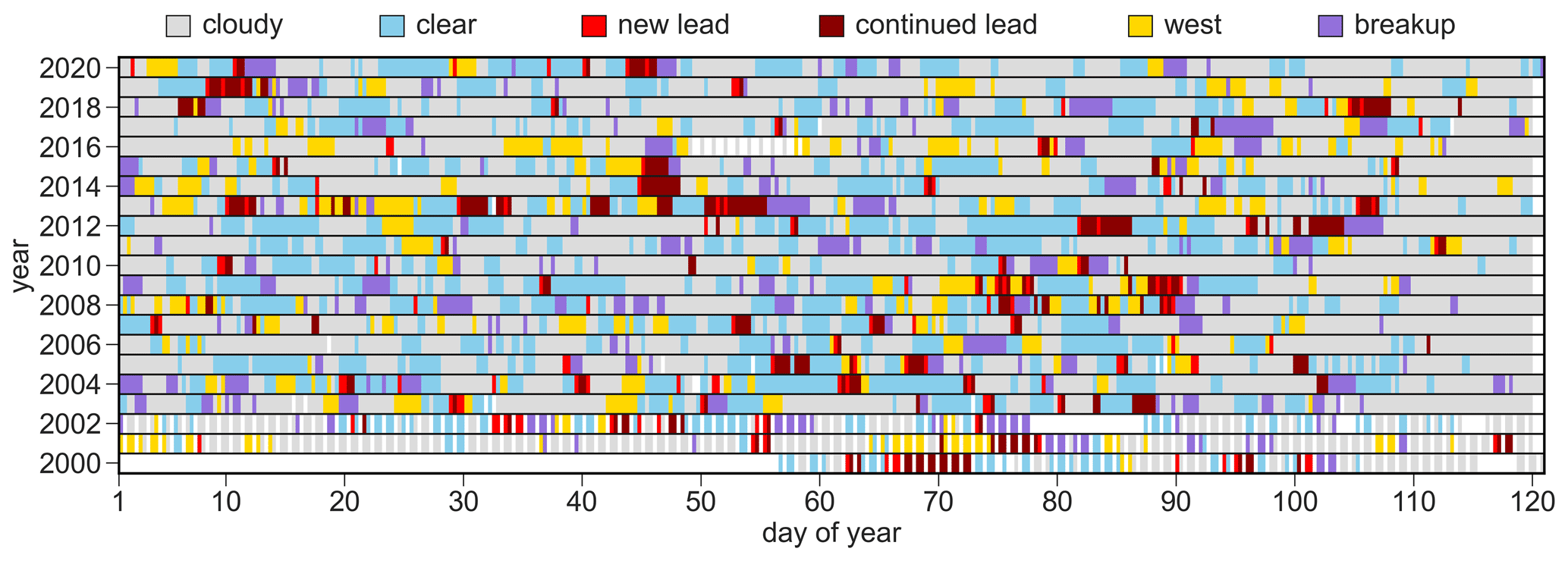
Figure A1 Three daily imagery categorizations over the analysis period. Colors indicate imagery category by year and day of year. White indicates no imagery.

Appendix B: Ensemble lead sequence calculations

B1 Determining the ensemble sequence window

The temporal window for the ensemble lead sequence was chosen for consistency in atmospheric conditions across events. To quantitatively evaluate the atmospheric consistency in the ensemble, the standard deviation in the daily SLP was calculated over the study domain across all distinct individual events in the ensemble from 5 d before to 5 d after the DLO (σ_event; N=82). This was compared to the climatological (January–April 2000–2020) standard deviation of daily SLP (σ_clim; N=2526) at every location to determine which days feature less ensemble variability than climatological variability. Figure B1 shows the ratio of σ_event to σ_clim from 5 d before to 5 d after the DLO.

The lowest relative SLP variability in the ensemble sequence occurs on the DLO and on DLO+1 as ${\mathit{\sigma }}_{\text{event}}/{\mathit{\sigma }}_{\text{clim}}$ dips below 0.8 over the central Arctic. The ensemble is therefore most representative of the atmospheric conditions across individual events on the days during lead opening. In most regions, σ_event increases relative to σ_clim with time before and after the DLO, indicating that the quality of the ensemble degrades with time from lead formation. From DLO−3 to DLO+2 in the ensemble sequence, the cross-event pressure variability remains lower than the climatological pressure variability over most of the Pacific Arctic Ocean, except over some coastal regions. This period is therefore chosen as the ensemble sequence. Outside this temporal window (on DLO−5, −4, +3, +4, and +5), σ_event exceeds σ_clim over portions of the Beaufort, Chukchi, and East Siberian seas, indicating that the atmospheric conditions are too variable in these regions to be considered in an ensemble.

B2 Calculating zonal mean lead positions

For the DLO, the mean and standard deviation in lead longitude were calculated as a function of latitude across identified patterns to quantify the average and zonal spread in the positions of opening. Due to the variable lengths of the lead patterns, the mean and standard deviation in the lead position become increasingly variable as the sample size used in the calculations decreases at higher latitudes (further offshore from their shared position at Point Barrow). To restrict analyses of the ensemble lead position to regions where it is still representative of most events, we only calculate the mean lead in the ensemble up to the latitude at which 70 % of the leads used in the ensemble calculation extend. Mean leads are calculated in this way for the full ensemble (Fig. B2a) across leads from the 82 distinct event sequences and for the wind direction ensembles (Fig. B2b–e) across leads that formed on non-overlapping days.

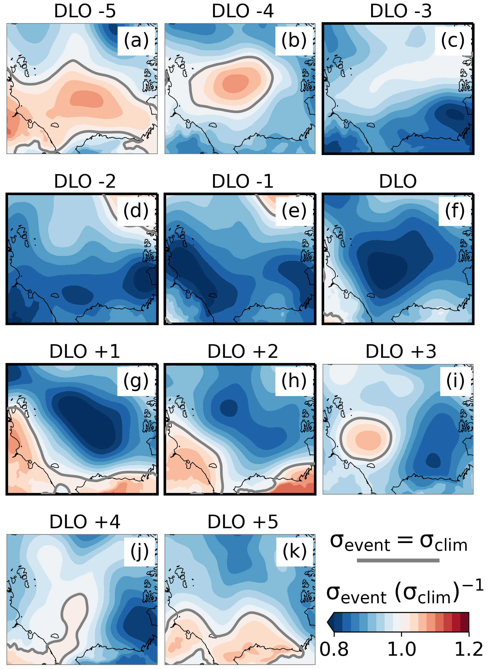
Figure B1 Ratio of the standard deviation in daily ensemble event SLP, σ_event, to the standard deviation in climatological daily SLP (January–April 2000–2020), σ_clim, for days −5 to 5 from the day of lead opening (DLO) in the ensemble lead sequence. Coastlines are underlain in black. Panels with a bold outline (c–h) are chosen for the lead sequence.

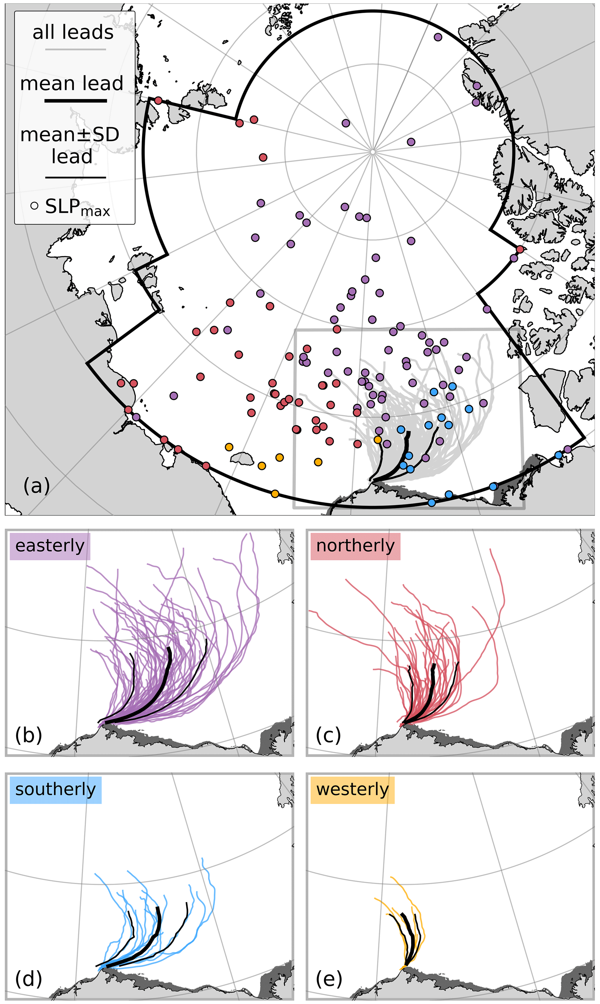
Figure B2 Distribution of atmospheric and lead conditions across events, which are sorted by wind direction. (a) All 135 lead patterns, which are overlain with the mean and the mean ± 1 standard deviation in the lead position across non-overlapping events. Points show the positions of SLP_max within the black outlined region from mean SLP fields of the 9 h windows preceding each lead identification. When multiple SLP_max are present, the nearest one to Point Barrow is displayed. Points along the region's boundary usually correspond to highs or ridges extending over the ocean from land. Dot colors correspond to the wind direction sorting shown in panels (b–e). Distribution of lead patterns formed under easterly (b), northerly (c), southerly (d), and westerly (e) winds are shown as colored lines, overlain with each group's mean lead and the mean ± 1 standard deviation. Alaskan landfast ice is shaded gray, as per Fig. 1.

Appendix C: Synoptic bias in cloud-free imagery

Identifying leads from cloud-free imagery could bias the synoptic conditions analyzed in the region and therefore those conditions that are determined to drive lead activity. To ensure that the identified differences in synoptic conditions between the lead events and climatological conditions are not artifacts of the requirement for low cloud cover, we compare winds and SLP in the BCS region from the climatology (all hours of the study period January–April 2000–2020) to those during low-cloud imagery and those during the identified lead events. These comparisons are depicted in Fig. C1, which demonstrates that the key differences in synoptic conditions between the climatology and lead events cannot be attributed to the method of lead identification.

There is little difference between the climatological and low-cloud wind distributions. The frequency of winds blowing from each wind quadrant during low-cloud images remains within ± 5 % of the climatological values, and the mean wind speed decreases to 4.8 ± 2.4 m s⁻¹ in low-cloud images from 5.0 ± 2.5 m s⁻¹ in the climatology. Mean SLP is biased 3.6 hPa high on average in the low-cloud imagery (1024.2 ± 10.6 hPa) when compared to the climatology (1020.6 ± 10.9 hPa). This is expected, given the association between cloudy conditions and decreasing SLP. Between the low-cloud imagery and the lead events, the distribution of wind directions changes substantially. For example, westerly winds during the events are 4 times less frequent than in the climatology and low-cloud images. In addition, mean SLP increases from that of the low-cloud imagery by 3.5 hPa (reaching 1027.7 ± 9.9 hPa). Mean wind speed decreases slightly to 4.5 ± 2.1 m s⁻¹.

The winds during low-cloud imagery are representative of the climatological conditions, wind direction changes considerably during the lead events, and the pressure bias in low-cloud imagery is surpassed during the lead events. We therefore conclude that the synoptic conditions associated with Point Barrow lead events are unique to the lead activity and are not influenced substantially by the method used to identify them.

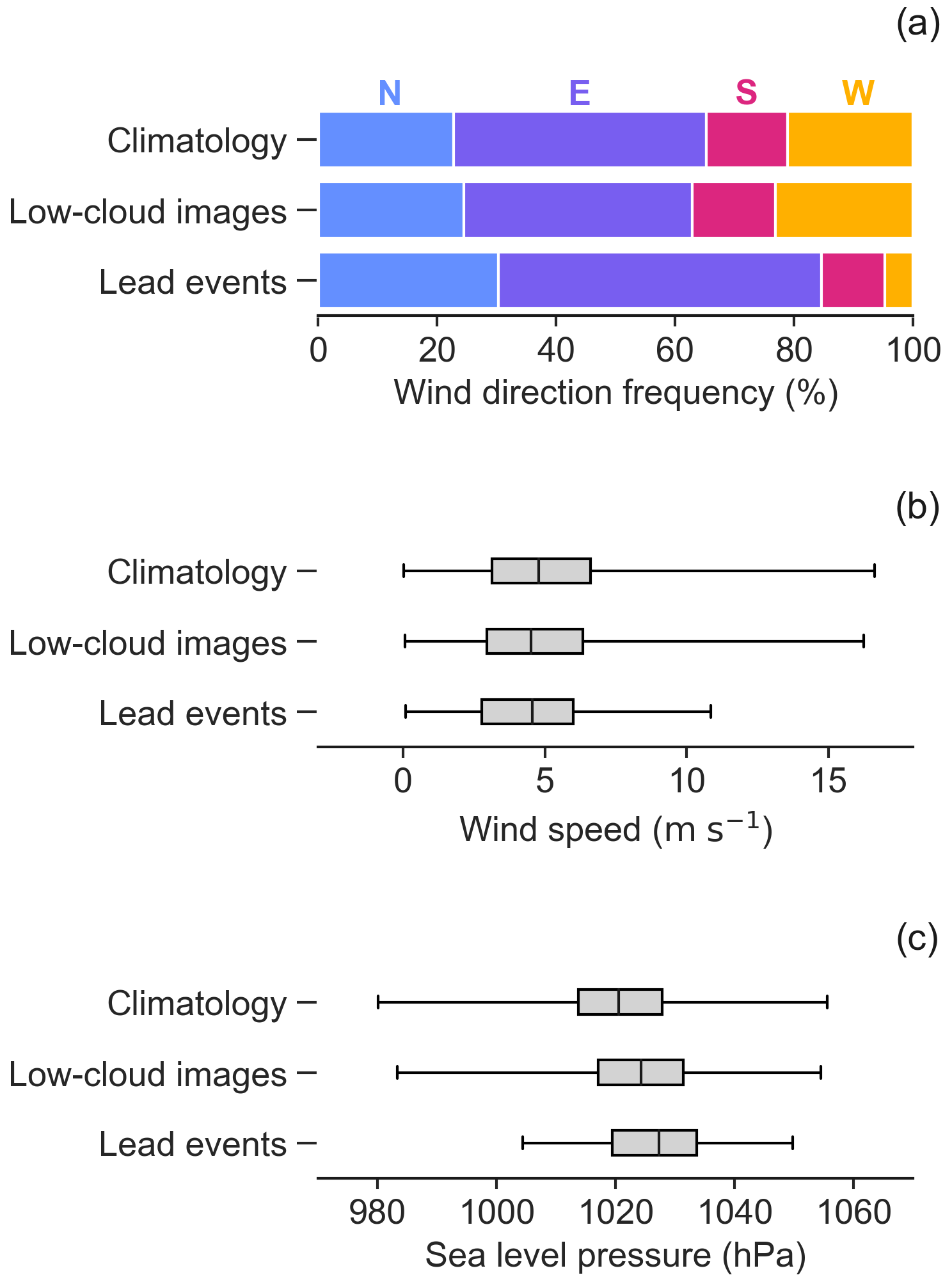
Figure C1 Comparison of synoptic conditions between all hours of the study (climatology), low-cloud images, and lead events. (a) Percentage of time that BCS winds originate from northerly (N), easterly (E), southerly (S), and westerly (W) directions for each category. Box-and-whisker plots of (b) wind speeds and (c) SLP in the BCS region for each category are shown. Whiskers show the minimum and maximum values. Boxes show the first quartile, median, and third quartile of the data.