Ice Sheet and Sea Ice Ultrawideband Microwave radiometric Airborne eXperiment (ISSIUMAX) in Antarctica: first results from Terra Nova Bay

An airborne microwave wide-band radiometer (500–2000 MHz) was operated for the first time in Antarctica to better understand the emission properties of sea ice, outlet glaciers and the interior ice sheet from Terra Nova Bay to Dome C. The different glaciological regimes were revealed to exhibit unique spectral signatures in this portion of the microwave spectrum. Generally, the brightness temperatures over a vertically homogeneous ice sheet are warmest at the lowest frequencies, consistent with models that predict that those channels sensed the deeper, warmer parts of the ice sheet. Vertical heterogeneities in the ice property profiles can alter this basic interpretation of the signal. Spectra along the lengths of outlet glaciers were modulated by the deposition and erosion of snow, driven by strong katabatic winds. Similar to previous experiments in Greenland, the brightness temperatures across the frequency band were low in crevasse areas. Variations in brightness temperature were consistent with spatial changes in sea ice type identified in satellite imagery and in situ ground-penetrating radar data. The results contribute to a better understanding of the utility of microwave wide-band radiometry for cryospheric studies and also advance knowledge of the important physics underlying existing L-band radiometers operating in space.

1 Introduction

Because Earth's polar regions are vast, remote and characterized by extreme environmental conditions, satellite sensors have been used extensively for monitoring changes in the surface properties, volume and extent of polar ice. Microwave sensors, both active and passive, are particularly suitable for this purpose due to their insensitivity to solar illumination and cloud cover. Since microwave penetration into polar ice increases with decreasing frequency, low microwave frequencies are required to observe inner properties of sea ice and ice sheets. Until the early 2000s, the lowest frequency available on polar orbiting satellites was C band (5.3 or 6.8 GHz for active or passive measurements, respectively) that limited ice sheet investigations to the properties of the upper 100 m of ice (Macelloni et al., 2007). With the launch of the L-band (1.4 GHz) SMOS (Kerr et al., 2010), Aquarius (Le Vine et al., 2010) and SMAP (Entekhabi et al., 2014) microwave radiometer missions, studies of deeper properties became possible. It is estimated that the 1.4 GHz brightness temperatures observed are sensitive to ice sheet properties down to 900 m (Macelloni et al., 2016). Over first-year sea ice (FYI), properties within 50 cm depth affect the L-band emission (Johnson et al., 2021). Estimations of sea ice thickness (SIT) (Kaleschke et al., 2012; Tian-Kunze et al., 2014) and ice sheet internal temperature profiles (Macelloni et al., 2016, 2019) have both been demonstrated using L-band brightness temperature measurements, although parameter estimations beyond the L-band penetration depth are extrapolations subject to increased uncertainty. Consequently, brightness temperature observations at longer wavelengths are a motivation to probe even further into sea ice and ice sheets. That said, the use of longer wavelengths is also challenged by the fact that the corresponding lower frequency ranges are allocated to other services by international regulations, (e.g., FCC allocation table, 2021), leading to radio frequency interference (RFI) for radiometric measurements. The development of advanced techniques for filtering RFI (as demonstrated for the 1400–1427 MHz band in the SMAP mission; Mohammed et al., 2016) has enabled the use of lower frequencies for monitoring polar regions even in the presence of other co-existing electromagnetic systems. Second, existing algorithms for geophysical parameters estimation are based on volume scattering, which is negligible at low microwave frequencies. Thus, new models are needed to interpret brightness temperature measurements and retrieve geophysical parameters.

A seminal paper aimed at describing in detail the physics of the low-frequency microwave emission of polar ice sheets and the benefits of using spectral measurements for estimating the temperature profile was published in 2015 (Jezek et al., 2015) followed by other papers focused on the Greenland ice sheet (e.g., Yardim et al., 2022a) and the sea ice in the Arctic region (e.g., Jezek et al., 2019; Demir et al., 2022b). A first airborne prototype (the Ultra-WideBand software defined RADiometer – UWBRAD) that observes brightness temperature spectra in the range 500–2000 MHz (Andrews et al., 2018) was developed under a NASA Instrument Incubator Program led by The Ohio State University. Two airborne campaigns were successfully conducted in Greenland in 2016 and 2017 that demonstrated the feasibility of ice sheet temperature retrieval, the potential for distinguishing glacier facies, and the retrieval of information on sea ice thickness and salinity (Andrews et al., 2018; Jezek et al., 2019, 2022; Yardim et al., 2022a). These campaigns also proved that polar geophysical measurements were possible in this frequency range when advanced RFI processing is used to enable “opportunistic” brightness temperature measurements in RFI-free portions of time and frequency space (Duan et al., 2022).

The success of the Greenland campaigns motivated a new set of UWBRAD measurements in Antarctica. With support from the Italian Antarctic Program (PNRA) and supplementary support from NASA, the “Ice Sheet and Sea Ice Ultrawideband Microwave Airborne eXperiment – ISSIUMAX” project was conducted in the austral spring of 2018. The project goals were (i) to provide additional demonstrations of the use of 500–2000 MHz brightness temperature spectra for deriving vertical ice sheet temperature profiles in the inner part of Antarctica and (ii) to demonstrate the capability of inferring glaciological information in coastal regions, including sea ice. An additional goal was to provide an additional demonstration that microwave radiometry is feasible in the heavily used 500–2000 MHz spectral range in remote regions such as Antarctica. The ISSIUMAX campaign took place between 30 October and 8 December 2018, from the Italian Antarctic base (Mario Zucchelli Station) on the Ross Sea. The campaign included the collection of airborne UWBRAD radiometer data over more than 5000 km of flight distance that was complemented by additional airborne and ground-based GPR (ground-penetrating radar) measurements and by satellite observations. Brogioni et al. (2022) reports and analyzes observations acquired in the inner part of the East Antarctic Plateau, and Andrews et al. (2021) describes the instrument design and RFI processing in detail.

This paper presents an overview of the campaign with a special emphasis on data collected in the coastal regions. The next section provides a brief description of UWBRAD, and the sites surveyed are summarized in Sect. 3. The planning and execution of the campaign are detailed in Sect. 4, and Sect. 5 describes the 500–2000 MHz spectral variations observed for a variety of geophysical scenes of interest.

2 UWBRAD dataset description

UWBRAD is the first ultrawideband radiometer measuring brightness temperatures simultaneously over the 0.5–2 GHz range through the use of 12 total ∼ 88 MHz bandwidth contiguous channels centered at frequencies from 560 to 1950 MHz and a circularly polarized nadir pointed conical log spiral antenna (Andrews et al., 2018). The antenna is designed to have an approximate 60^∘ half-power beamwidth that is independent of frequency so that all frequency channels observe a similar region on Earth's surface. This beamwidth results in a 3 dB footprint on Earth's surface whose diameter is approximately 15.5 % greater than the aircraft altitude above the local terrain. For the ISSIUMAX campaign, the nominal flight altitude was in the 500–600 m range, and the average altitude was 541 m, resulting in a typical footprint diameter of 625 m. At the nominal flight velocity of 240 km h⁻¹, this footprint remains Nyquist sampled (i.e., two measurements per footprint) at an integration time of approximately 4.5 s.

The UWBRAD radiometer performs two different kinds of calibration. The internal calibration process described in Andrews et al. (2018) is used to compensate for the impact of changes in system temperature or receiver gains on measured data by means of the measurements of internal known loads. An external absolute calibration is then performed for each flight based on the use of known targets, i.e., the coastal moraine and the open ocean as hot and cold reference targets, respectively. Before applying the external calibration, RFI detection is performed through a combination of algorithms as detailed in Andrews et al. (2021). A description of the UWBRAD calibration process and RFI detection is also provided in Appendix A.

The datasets shown in what follows are integrated over five samples representing an integration time of ∼ 5 s. Studies of the resulting 12 channel brightness temperatures over relatively homogeneous scenes show local variations having standard deviations from ∼ 0.25 to ∼ 1 K that vary with frequency and with the RFI environment at the time of the measurement. However, because the final external calibration of each frequency sub-channel remains uniform over an entire flight duration, any instabilities in the instrument frequency response can impact the frequency response of the resulting calibrated brightness temperatures. Such effects are estimated to be within ±5 K based on an extensive analysis of the final dataset.

Figure 1 provides an example of the resulting 6144 point frequency spectra for 21:05–21:35 UTC on 24 November (i.e., 10:05–10:35 LT on 25 November) before (upper left) and after (upper right) the iterative RFI filtering and external calibration procedure. The correction or filtering of multiple spectral anomalies is evident, along with the associated loss of some portions of the measured spectrum for use in producing the final integrated products. The corresponding 12 channel-integrated products for this time period are illustrated in the lower-right plot and show transitions from open water to coastal ice scenes having a variety of spectral features as described in what follows. The lower-left portion of Fig. 1 is a photograph of UWBRAD after installation on the Twin Otter aircraft operated by Kenn Borek airlines. Visible in the photograph are the “periscope” system from which the conical spiral antenna is deployed after takeoff and the electronics rack containing the UWBRAD radiometer receiver and data-processing computers.

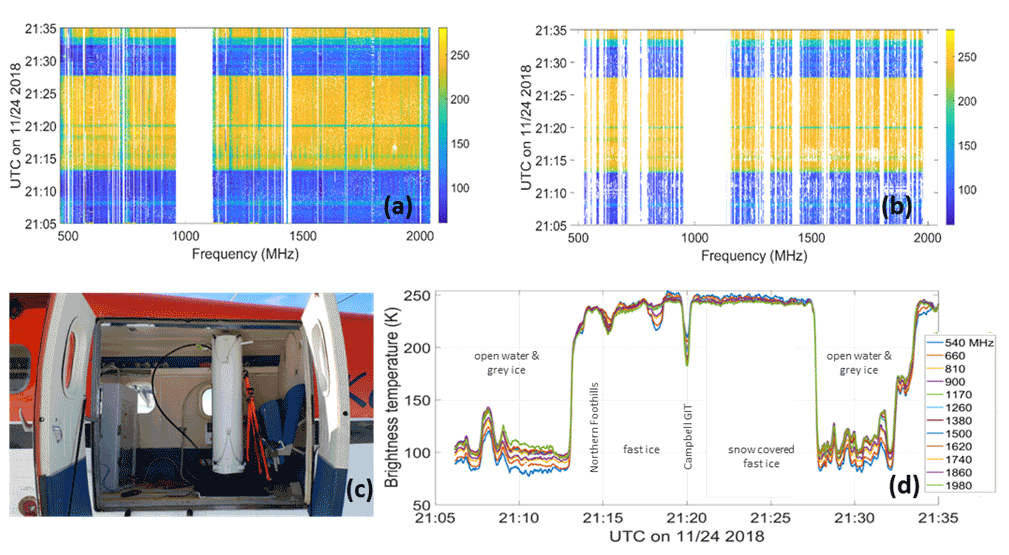
Figure 1 (a, b) The 6144 frequency channel spectrograms of brightness temperatures (in K) before (a) and after (b) application of the iterative RFI filtering and external calibration procedure. (c) Photograph of UWBRAD antenna periscope and equipment rack aboard Twin Otter aircraft of Kenn Borek Airlines. (d) The 12 channel-integrated brightness temperatures corresponding to the spectrograms shown in the upper plots. Labels indicate type of targets observed along the transect.

3 Test sites

The ISSIUMAX campaign took place in Victoria Land, East Antarctica, where the Italian Antarctic Program (PNRA) operates two stations: Mario Zucchelli Station (MZS, 74.695^∘ S, 164.114^∘ E), situated in Terra Nova Bay (TNB) on the western coast of the Ross Sea, and Concordia Station (75.1^∘ S, 123.33^∘ E, operated in cooperation with the French Polar Institute Paul-Émile Victor, IPEV), located at Dome C on the East Antarctic Plateau at an elevation of 3233 m. Both stations were used as starting points for UWBRAD flights, but the analyses reported in this paper are for measurements collected in the coastal region only. Preliminary results obtained on the ice sheet plateau further inland and close to Concordia Station are reported in Brogioni et al. (2022).

Terra Nova Bay is bounded by the Drygalski Ice Tongue to the south, Cape Washington to the north, the East Antarctic Plateau to the west, and the Ross Sea to the east. MZS is located on the coastal Northern Foothills range and is separated from the ice sheet by the Transantarctic mountains (Fig. 2). The geography contains many glaciological features of interest in the campaign, including the Priestley, Reeves, and Campbell glaciers (which feeds the Campbell Glacier Tongue); David Glacier and the related Drygalski Ice Tongue, and sea ice around Cape Washington. The former two glaciers feed the Nansen Ice Sheet, which is actually an ice shelf and is referred to as such throughout the paper for sake of clarity. The mean annual temperature in the region is −14 ^∘C, with January (mean temperature −2 ^∘C) being the warmest month and May or August (−23 ^∘C) the coldest months (Frezzotti et al., 2001). Sea ice in the region is usually first-year fast ice (FYI) and is typically 2 m thick close to the coast (Rack et al., 2021), and this ice vanishes in December due to a combination of processes: late spring air temperature increases the ice temperature and the brine volume that acts to weaken the fast ice (Frankenstein and Garner, 1967; Weeks and Ackley, 1982), then long-wavelength sea swell due to offshore storms break the pack, which in turn is moved offshore by the katabatic winds (e.g., Bromwich and Kurtz, 1984).

Occasionally, fast ice can remain in place for more than 1 year at some sites, for instance in the inner parts of Silverfish Bay, Wood Bay or Tethys Bay. In this case the multi-year landfast ice (MYI) can reach a higher thickness of 3–4 m, as encountered in the campaign.

Figure 2 Map of Terra Nova Bay. The planned routes of flights 1 and 2 are represented in red and green, respectively. The yellow star indicates the location of Mario Zucchelli Station (MZS). The background image is a mosaic of Landsat 8 RGB composites collected on 24 November (coastal zone, contemporary to the flight) and 27 November (inland portions).

4 Campaign planning and execution

Flight routes were planned based on the flight time assigned to the project (35 flight hours divided among radiometric and ground-penetrating radar measurements) and coverage of the following areas:

• sea ice in Terra Nova Bay and Wood Bay;

• the Nansen Ice Shelf and related inlet glaciers;

• the ice sheet along the paths from MZS to Concordia Station and MZS to Talos Dome (73.0^∘ S, 158.0^∘ E);

• other secondary targets such as buried lakes, open sea, exposed outcrops (e.g., nunataks and moraines), and blue ice.

Sea ice flights were planned based on the known presence of grease ice or nilas bands and fast ice, as well as the expectation of highly stable FYI and minimal multi-year ice (about 1.5–2 years), at these locations. MYI was identified by analyzing long time series of MODIS and Sentinel-1 images. Complementary flights of a helicopter-mounted 400 MHz GPR were made in order to achieve additional information about the electromagnetic response of the sea ice and its snow cover.

The final plan specified six flights of 5 h each. Flight 1 was planned to focus on sea ice and included many transects over the Gerlache Inlet, Silverfish Bay and Wood Bay (Fig. 2). The transects were designed to survey sea ice in directions both parallel and orthogonal to the coast in order to capture the variability of the sea ice thickness (SIT) and ice type. The inner part of Wood Bay is characterized by very thick fast ice (FYI or MYI of approximately 3 m thickness), whereas the outer part of the bay contains FYI of ∼ 2 m thickness. The external part of the bay in contrast hosts nilas and grease ice. Sea ice in Wood Bay is usually snow covered. Silverfish Bay and the Gerlache Inlet are instead covered almost entirely by 2.0–2.5 m thick FYI and usually experience different dynamics given the katabatic winds at these locations that remove snow from the surface.

Flight 2 was planned primarily to observe terrestrial ice inland from MZS. The flight surveyed the Priestley Glacier along the route of a 2013 Operation Ice Bridge (OIB) survey (from which information on the inner structure of the glacier can be obtained) and then proceeded over the ice sheet toward the David Glacier. Results from flights 1 and 2 are the subject of this paper.

Flight 3 was designed to collect data over the Antarctic ice sheet and followed the route of the ITASE 98/99 traverse. Flight 4 was planned to collect data over glaciological features in the vicinity of Concordia Station, including Aurora Basin (150 km north of Concordia Station), which is characterized by deep trances in the bedrock and a network of subglacial lakes such as Concordia Lake. Little Dome C, the site of the Beyond EPICA – Oldest Ice project drilling, was also surveyed (Augustin et al., 2004); the topography of this site is known in detail (Young et al., 2017), and several temperature profiles of the ice are available (Ritz et al., 2010). The return flight 5 from Concordia Station to MZS was planned to survey the megadune region in the East Antarctic Plateau (Frezzotti et al., 2002; Courville et al., 2007), multiple blue ice sites and buried lakes in the coastal region. Brogioni et al. (2022) provides a detailed description of these inland flights.

The campaign was organized in phases. The first phase included the collection of GPR surveys and in situ measurements of sea ice (3–18 November). Acquisition of radiometric data for the coastal area (24–25 November) followed, along with sky calibration measurements (29–30 November). Finally, measurements were completed over the inland ice sheet (2–5 December).

4.1 GPR surveys

The activities scheduled for the first part of the campaign were carried out using a GPR instrumentation (GSSI Sir3000) equipped with a 400 MHz helicopter-mounted antenna. The instrument has a 150 ns investigation range with a 16 bit sampling. The helicopter's average speed was about 40 kn, which implies the acquisition of a single trace about every 28 cm and calculated vertical resolution (into the ice) of about 32 cm. Considering that flight height was about 4–5 m, the time range allowed an ice penetration of about 10–11 m. The aim of GPR survey was to collect measurements of sea ice thickness in the Gerlache Inlet, Silverfish Bay, Wood Bay, and the ice structure along a path between the Nansen ice shelf and the Priestley Glacier (Fig. 4). The planned GPR flight lines were to be repeated at least three times to study any progressive increase in brine volume of the ice as it warmed (Frankenstein and Garner, 1967). Preparation and assembly of the GPR and related instruments occurred from 30 October to 2 November, and on 3 November the first survey covering the area between MZS and Cape Washington was acquired (Leg 1: TNB and Silverfish Bay; shown in red in Fig. 3). Cloud cover was continuously present in the region until 7 November that prevented flights until 9 November when measurements were performed over Wood Bay (Leg 2, purple line in Fig. 3) and repeated for Leg 1. A flight over Leg 3 (blue line in Fig. 3) was performed on 12 November, followed by a repeat of Leg 1, Leg 2 and part of Leg 3 on the sea ice on 18 November.

The survey benefitted from the presence of several sea ice coring holes in Silverfish Bay and Gerlache Inlet that were used as a reference for depth conversion of GPR data. In addition, on 18 November sea ice and seawater were sampled in Silverfish Bay for salinity measurements by using a COND61 XS Instruments Italy device (calibrated with proper standard solutions). The results showed sea ice salinities of 6.14, 6.35 and 7.56 g kg⁻¹ at 0.6, 2 and 2.8 m depths, respectively, while the seawater below the ice ranged around a value of about 31.8 g kg⁻¹ (yellow triangle in Fig. 3). Other seawater salinity measurements conducted in Gerlache Inlet showed values between 31.2 and 32.1 g kg⁻¹ (cyan triangles in Fig. 3).

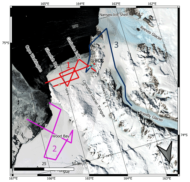
Figure 3 GPR flight routes. Leg 1 traveled across Terra Nova Bay and Silverfish Bay (red lines), Leg 2 traveled across Wood Bay (purple lines), and Leg 3 traveled from Priestley Glacier to the Gerlache Inlet (blue lines). Cyan triangles indicates the seawater salinity test sites, and the yellow triangle marks the site of the sea ice salinity measurements.

4.2 UWBRAD surveys

UWBRAD was installed on board the Twin Otter aircraft on 24 November, and the first and second flights were performed on 25 November. The flight's route included 41 waypoints plus a further 4 that overlapped ICESat-2 measurement tracks. The aircraft departed MZS at 09:30 LT towards a polynya that had formed north of the Drygalski Ice Tongue (to enable open-water calibration measurements), and measurements concluded at approximately 13:00 LT when the aircraft landed at MZS for refueling. During this flight, the air temperature recorded by the automatic weather stations (AWSs) at MZS ranged from −4 to −2 ^∘C. Other AWS sites, e.g., at Cape King (73.586^∘ S, 166.621^∘ E) and Boulder Clay (74.751^∘ S, 164.021^∘ E), reported 1–2 ^∘C cooler temperatures. Flight 2 then began at 15:00 LT with the aircraft proceeding inland along the Priestly Glacier. The flight proceeded according to the planned route until reaching the Reeves Glacier when, due to adverse wind conditions in the region, it was decided to eliminate the two transects from the Nansen Ice Shelf toward the Drygalski Ice Tongue. Due to this change, it was possible to perform two other transects of sea ice in Wood Bay along the ICESat 2 satellite tracks. Flight 2 was completed with the return to MZS at 19:20 LT. The final flight paths achieved are shown in Fig. 4.

On 29 November, the microwave radiometer was installed on the ground near the Oasi shelter (away from the main MZS buildings) in order to perform sky-viewing calibrations (Andrews et al., 2021). The data collected were used to perform calibration tests and studies of RFI. These measurements continued on 30 November with varying levels of additional attenuation placed on the radiometer antenna and concluded on 1 December.

Flight 3 towards Dome C began at 22:26 UTC on 2 December and a transect over one of the ESA DOMECair experiment routes was performed before landing at Concordia Station to allow intercomparisons with the 1.4 GHz brightness temperatures previously acquired by the EMIRAD sensor (Kristensen et al., 2013). Flight 4 over Little Dome C and two other DOMECair flight lines then occurred on 3 December from 05:25 to 09:32 UTC. The flight 5 return to MZS was performed on 5 December. On this flight, UWBRAD acquired data only for the Mid Point–Terra Nova Bay route.

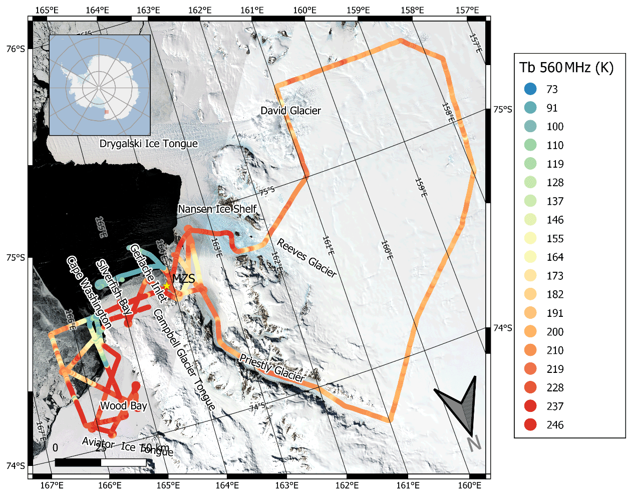
Figure 4 Map of flights 1 and 2 as executed over the coastal regions. Colors represent the UWBRAD brightness temperature (T_b) measured at 560 MHz. The background image is a mosaic of Landsat 8 RGB composites collected on 24 November (coastal zone, contemporary to the flight) and 27 November.

4.3 Summary of datasets

The final UWBRAD dataset of geolocated nadir brightness temperatures in 12 frequency channels covers a distance of more than 5200 km. The GPR dataset covers the sea ice region and was collected prior to the radiometric flights. However, no major sea ice dynamic events were observed prior to the coastal UWBRAD flights so that the two datasets can be reasonably compared. GPR data were acquired over sea ice having a thickness of 2 m or more that is expected to remain fast until major breakup events at the beginning of December.

Datasets from other spaceborne remote sensing instruments were also assembled for intercomparison; see the detailed list of data sources in Appendix B. Both optical (e.g., Landsat-8 and Sentinel-2) and radar (e.g., ALOS, Sentinel-1 and COSMO-SkyMed) datasets were collected over all the flight routes. Mosaics available through the Quantarctica collection (Matsuoka et al., 2021) were also examined, including the RAMP project Radarsat mosaic (Jezek, 1999; Jezek et al., 2013) and the Landsat Mosaic of Antarctica (Bindschadler et al., 2008). Ice sheet thickness information was also obtained from the Bedmachine project (Morlighem et al., 2020), and geothermal heat flux estimates were obtained from Fox Maule et al. (2005).

5 Results

The brightness temperature spectra acquired by UWBRAD respond to the properties of the medium observed. Expectations for properties of brightness temperature spectra and their trends versus frequency for common targets will be used to interpret the results that follow. For example, typical “water” and “thin sea ice” spectra show an increasing trend versus frequency given the dielectric properties of seawater and the decreased electromagnetic loss through thin sea ice at lower frequencies. “Ice sheet” spectra in contrast decrease with frequency due to the sensitivity of lower frequencies to the warmer ice at greater depths. Both cases can further be impacted by any scattering effects within the medium observed, which typically would be expected to decrease observed brightness temperatures and to have a greater impact on higher frequencies. The scatterers producing such effects must be of a size that is appreciable compared to the wavelength, i.e., of at least approximately centimeter scales so that the impact of features such as snow grains can typically be neglected. Scatterers of these sizes are more likely to occur in portions of the snow or firn that experience periodic melt and refreeze events, as discussed in Jezek et al. (2017). All of these physical effects are evident in the initial examples presented in what follows. These results provide evidence of the information contained in measurements of brightness temperature spectra in coastal Antarctica, including scenes containing sea ice, glaciers, rocks, ice shelves and subsurface lakes.

5.1 Sea ice

A first example highlighting the spectral behavior of different sea ice types comes from a flight 1 transect that passed from Gerlache Inlet to Silverfish Bay (left plot of Fig. 5). An analysis of a 1-year time series of Sentinel-1 synthetic aperture radar (SAR) images showed that the near-coastal sea ice (or “fast ice”) at sites 1, 3 and 5 in Fig. 5 formed in March–April 2018. GPR measurements reported an ice thickness of 2.0–2.5 m. Katabatic winds near site 1 cause ablation and sublimation of the fast ice and result in almost no snow coverage, while the fast ice at sites 3 and 5 was covered by snow of less than 45 cm thickness (estimated from GPR data). The same Sentinel 1 analysis showed that the “outer region” sea ice at site 2 in contrast was the product of multiple breakup processes. This ice at the time of ISSIUMAX formed in September composed by old small floes and newly formed ice. The GPR survey showed an average thickness of only 1.5 m in this region, along with evidence of relative increase in brine volume of the ice at site 2. The site 4 ice of the Campbell Glacier Tongue, which is inland glacier ice that flows through the Transantarctic Mountains and then over the sea, therefore has a much greater thickness (about 400 m at the hinge point; Han and Lee, 2014) and distinctly different dielectric properties. Indeed, this continental ice is generated by the accumulation of snow on the plateau over centuries and can be considered to be pure ice with very small losses, as opposed to the sea ice of the other sites that is characterized by high dielectric losses due to the inclusion of saline brine pockets. These differences significantly impact microwave penetration through the ice and therefore the ice properties sensed by UWBRAD (Demir et al., 2022a).

A time series of UWBRAD brightness temperatures is provided in Fig. 6a, along with brightness temperature spectra at the five labeled sites in Fig. 6b. As expected from theory (Demir et al., 2022a; Johnson et al., 2021), the thicker sea ice at sites 1, 3 and 5 shows a “flatter” spectrum, having brightness temperatures in the 240–250 K range. This is due to the sensitivity of brightness temperature to ice thickness: for a salinity of 6 g kg⁻¹ (as measured in situ) the electromagnetic (EM) signal saturates for thicknesses higher than 1.5–2 m even at 500 MHz. The flattest spectrum occurs for the bare ice at site 1, while the spectra of sites 3 and 5 show a slight decreasing trend with frequency. These small differences may be due to the impact of a depth hoar layer within the snow and/or differing temperature profiles inside of the ice caused by snow thermal insulation. However, routine measurements made by MZS on the sea ice near the airstrip revealed an ice temperature in the −5 to −2 ^∘C range at depths to 30 cm below the surface, meaning that the ice was almost isothermal at least to 30 cm depth (MZS operations room, personal communication, 15 January 2022).

Over the more dynamic and thinner ice at site 2, brightness temperatures show the expected lower values associated with an increase with frequency that was also observed in UWBRAD's Greenland campaign where the ice was typically thinner than 2 m (Jezek et al., 2019). At site 2, the presence of higher brine volume within the ice may also impact this result because the greater penetration at lower frequencies results in a greater sensitivity to the higher brine volume seen at greater depths than at higher frequencies.

Brightness temperatures over the glacier tongue (site 4) decrease uniformly with frequency from ∼ 210 K (560 MHz) to 182 K (1950 MHz). This behavior is typical of continental ice (Jezek et al., 2015; Yardim et al., 2022a; Brogioni et al., 2022) as described previously. The smooth transition of brightness temperatures observed in Fig. 7 during the overpass of the ice tongue is due to the large antenna footprint of UWBRAD. The spectra of Fig. 6b were obtained by averaging acquisitions in the vertically shaded portions of Fig. 6a that correspond to approximately uniform regions in space.

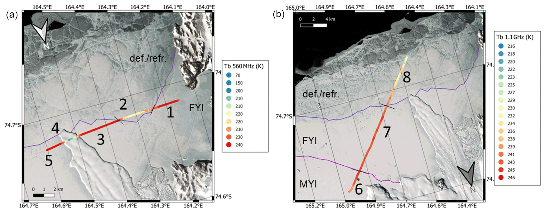
Figure 5 (a) Map of the transit from Gerlache Inlet to Silverfish Bay. Fast ice is present at sites 1 (FYI), 3 (FYI), and 5 (FYI); thinner deformed or refrozen ice is present at site 2; and site 4 marks the Campbell Glacier Tongue. (b) Map of transit from Silverfish Bay toward open sea. Pink and purple lines delimit MYI fast ice, FYI fast ice, and deformed or refrozen sea ice. The base map of both panels is a Landsat 8 RGB composite acquired contemporaneously with the flight.

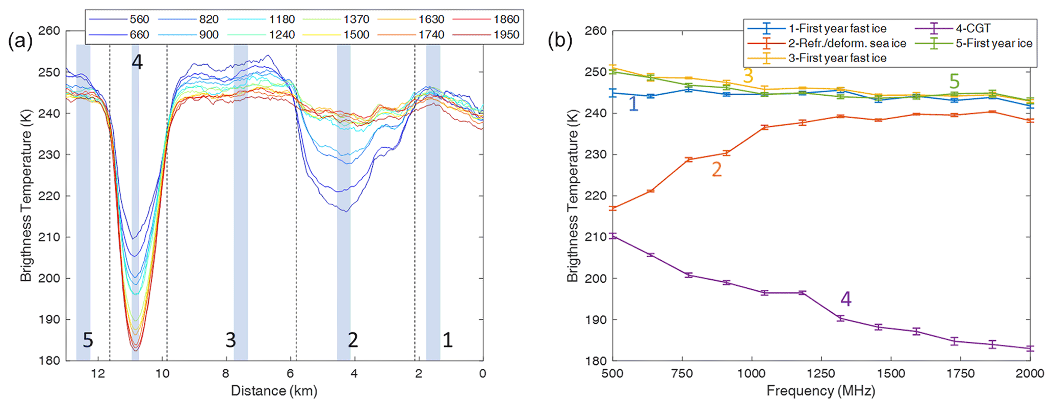
Figure 6 (a) Transect of UWBRAD brightness temperatures corresponding to the left panel of Fig. 5; the legend indicates the frequency (in MHz) of the 12 UWBRAD channels. (b) Spectra of the five different targets obtained as an average of data shaded in blue.

The right portion of Fig. 5 displays the flight path of a similar example that proceeds from Silverfish Bay toward the open sea beyond the tip of the Campbell Glacier Tongue (CGT). The transect begins over multi-year ice and proceeds toward the thinner ice to a refrozen sheet of pack or fast ice.

The ice thickness along this path is estimated by GPR measurements to be in the range 2.0–2.5 m for the majority of the transect (Fig. 7 bottom panel). As shown in Fig. 7, brightness temperatures over the multi-year (site 6, 0–4 km along the flight path) and first-year fast ice (site 7, 4–14 km) are near 245 K, although the MYI tends to be slightly cooler than the FYI fast ice (note that some channels in the earlier part of the plot are missing due to a reboot at this time of one of UWBRAD's data acquisition computers). For both site 6 and 7, the ice thickness estimated by GPR is greater than 2 m, meaning that brightness temperatures are again saturated as for similar sites in Fig. 6. As in the previous example, lower-frequency channels show slightly higher brightness temperatures (by ∼ 2–4 K) than higher frequencies. GPR measurements over site 6 (shown in Fig. 7b and interpreted into snow and ice thicknesses in the Fig. 7c) confirm the presence of multi-year ice (nearly second year ice, dated by using satellite images) for which the scattering within the ice or at the ice–water interface was quite high, meaning that brightness temperatures are moderately lower than those at site 7 where GPR measurements show much lower evidence of scattering. Differences between these two sites may also be related to a lower brine content in the MYI at site 6 as compared to the FYI at site 7. This is confirmed also by measurements collected over Wood Bay (Fig. 8), where the T_b of MYI (identified by pink contours) is cooler than T_b over first-year fast ice (delimited by the purple line).

Brightness temperatures at site 8 are similar to those at site 2, and there is evidence of increased scattering and the percolation of seawater into the snow–ice interface. As at site 2, brightness temperatures increase with frequency, likely due to the infiltrated water's impact. SAR backscatter measurements from Sentinel-1 (C-band) and COSMO-SkyMed (X-band) are also included for this transect and show a response that is negatively correlated to brightness temperatures, as should be expected when either surface- or volume-scattering effects are present within the ice observed (although the influence of particular scatterers should be expected to increase with frequency).

Figure 7 (a) Time series of UWBRAD and SAR data as a function of position along the path in Fig. 6a. (b) Echogram obtained by GPR along with visual interpretation. (c) Sea and snow thickness estimated from GPR data. Some UWBRAD data are missing in the first 8 km due to an unexpected computer reboot.

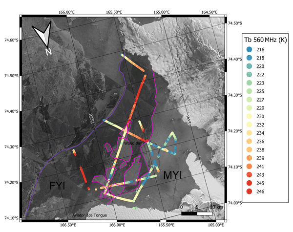
Figure 8 Map of the transects over the inner part of Wood Bay. Pink and purple lines delimit MYI (2 years) and FYI fast ice, respectively. The base map is a mosaic of COSMO-SkyMed X-band SAR images acquired on 21 and 27 November 2018 (4 d before and 3 d after the flight, respectively).

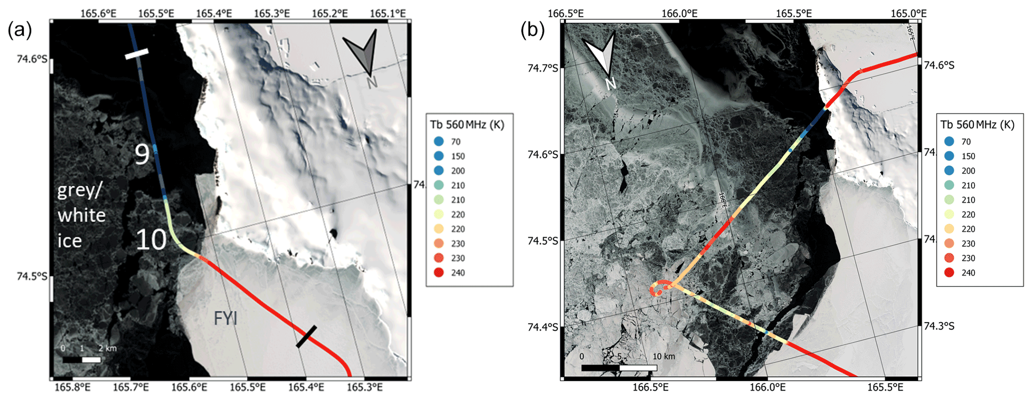
Figure 9 (a) Map of the transit from Cape Washington to Wood Bay; white and black marks indicate the beginning and end of the transect, respectively. (b) Map of the transit from Wood Bay to Cape Washington. The base map is a Landsat 8 RGB composite acquired contemporary to the flight.

A third example was acquired in Wood Bay as the aircraft moved from open water to fast ice passing through a grey and white ice field (Fig. 9, left). As discussed previously, sea ice in Terra Nova Bay in November–early December is characterized by near-coastal FYI fast ice of 2–3 m thickness surrounded by nilas and gray ice in some cases (Mezgec et al., 2017; Brett et al., 2020). Occasionally MYI is present very close to the coast. The path shown begins over open water (low brightness temperature), then enters the grey and white ice region, and finally arrives over thick ice of about 2.5 m thickness. Over this transect the ice was free of snow. Brightness temperature time series along this path are shown in Fig. 10a, with spectra for selected locations shown in Fig. 10b. The difference between site 9 and site 10 appears to be influenced by the ice concentration within the UWBRAD footprint and potentially any differences in ice thickness at these locations. Spectra for the two sites show an increasing trend similar to that observed for open water but have a mean value that increases as the ice concentration increases and a saturation at a frequency that shifts toward lower frequencies as the ice concentration increases. The spectrum for the thicker ice in this region is flat, with an average brightness temperature of 240 K, as is the case for the snow-free ice at site 1 in Fig. 5.

A final sea ice example includes a passage from fast ice of 2.5–2.7 m thickness to a young ice field as the airplane returned to Silverfish Bay from Wood Bay (Fig. 9b). The background image in this plot is a Landsat 8 RGB composite acquired 2 h before the Wood Bay survey. Given the weak sea currents in the bay expected at this time, the image provides a reasonable representation of the ice at the UWBRAD acquisition time. The brightness temperature time series for this transect is shown in Fig. 10c, along with the panchromatic and thermal IR data from the Landsat 8 product. The high correlation observed between the panchromatic data and brightness temperature variations provides further evidence that the Landsat 8 image is suitable to support the interpretation of UWBRAD acquisitions. Depending on the ice concentration and thickness, brightness temperatures vary from ∼ 120 to ∼ 240 K. Note that young ice is typically much more saline than FYI, reaching salinities up to 12–15 g kg⁻¹ (Cox and Weeks, 1974) so that brightness temperatures saturate for shallower ice thickness. By using Landsat 8 IR data and the thermodynamic model described in Maykut and Untersteiner (1971); Yu and Rothrock (1996); Drucker et al. (2003), it is possible to estimate ice thickness in the young ice field. The air temperature, required for this analysis, was derived from the MZS AWS and the ECMWF ERA5 reanalysis (Hersbach et al., 2018, 2020), while the superficial ice temperature was obtained from the Landsat thermal infrared (TIR) bands. Note that this method is applicable for ice up to approximately 50 cm thickness in stationary conditions. Moreover, since a validation of the retrieved ice thickness is not possible, we consider values obtained as a proxy for assessing the dependence of UWBRAD brightness temperatures on SIT.

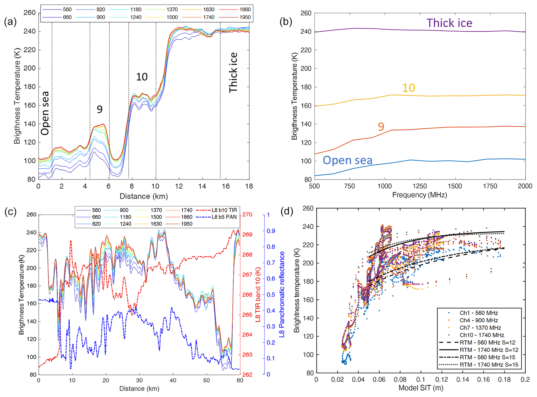
Figure 10 (a) Time series of brightness temperature corresponding to Fig. 9a. (b) Spectra of four selected targets from Fig. 9b. (c) Time series of UWBRAD brightness temperature, surface temperature derived from band 10 TIR of Landsat 8 (red), and reflectance derived from band 8 panchromatic data of Landsat 8 (blue) for the transect in Fig. 9b. (d) Scatterplot of UWBRAD channels 1, 4, 7 and 10 versus estimated sea ice thickness, along with an EM radiative transfer model estimation for T_ice of −4 ^∘C, T_water of −2 ^∘C, and salinity of 12 (continuous and dashed lines) and 15 g kg⁻¹ (dotted and dashed–dotted lines).

Figure 10d plots the UWBRAD brightness temperatures in four frequency channels versus the retrieved ice thickness; the predictions of a radiative transfer model for brightness temperatures are also included. Radiative transfer model (RTM) simulations assume a finite-thickness slab of sea ice over water, and the calculation starts from a minimum thickness of 5 cm since for lower values the incoherent model fails to correctly simulate the EM emission. In reality, layers thinner than a quarter of the wavelength (about 15 cm at 0.5 GHz and 3.5 cm at 2 GHz) cannot be treated with a conventional or simple wave propagation approach, and a coherent RT should be used (which requires a highly accurate characterization of the medium surfaces seldom available in such scenarios). As expected, a rapid increase in brightness temperature at all frequencies versus ice thickness is observed. It should be noted that shallow young ice has a brightness temperature similar to thick FYI due to its increased brine content and electromagnetic losses. Young ice is shallower than FYI but with a higher salinity, resulting in similar brightness temperatures. While the four frequency channels shown appear to respond similarly, at 560 MHz a lower brightness temperature is reached at the maximum thickness as compared to the other higher channels, suggesting that further sensitivity to ice thickness is available (though not for the limited ice thickness available along this transect). The curves in Fig. 10d represent simulated data that were obtained by using an electromagnetic radiative transfer model (Picard et al., 2013): the ice is assumed to be a homogeneous layer whose permittivity is obtained from Vant et al. (1978) overlying a semi-infinite medium representing seawater (Klein and Swift, 1977). The ice temperature is assumed −4 ^∘C (average temperature recorded by the AWS at MZS and Cape King), while the ice salinity is 12 and 15 g kg⁻¹ (typical values for young ice). Simulated trends show reasonable agreement with the sensitivity of the experimental data (better for a salinity of 12 than 15 g kg⁻¹), indicating that the sensitivity of brightness temperature to ice thickness is strongly affected by the brine content of the ice (with higher ice salinities reducing sensitivity to ice thickness as expected). This result has implications for SIT estimation from satellite measurements and confirms the importance of ice salinity information in the thickness retrieval process.

All the examples previously described illustrate the sensitivity of 500–2000 MHz brightness temperature spectra to a variety of sea ice properties including ice thickness, salinity, snow cover, and the presence of scattering or higher brine volume (driven by higher salinity) within thin ice. Because of the natural heterogeneity of sea ice, these effects should be expected to be more significant in the ∼ 625 m footprint of UWBRAD as compared to the 40–60 km spatial footprints obtained from the current satellite observations of missions such as SMOS and SMAP.

5.2 Glaciers

In the Terra Nova Bay region, glaciers flow outward from the Transantarctic Mountains toward the sea. For instance, Priestley Glacier flows for about 120 km from the eastern part of Victoria Land into the Ross Sea and feeds the Nansen Ice Shelf. Priestley Glacier was surveyed in 2013 by OIB's Multichannel Coherent Radar Depth Sounder (MCoRDS) and accumulation radar. The UWBRAD route of flight 2 was aligned with these OIB transects (Fig. 11). Given Priestley Glacier's velocity of about 100 m yr⁻¹ (Frezzotti et al., 2000; Mouginot et al., 2012), a displacement of about 500 m should be expected between the OIB and UWBRAD data. This displacement, which corresponds roughly to one UWBRAD footprint, is neglected in what follows.

Figure 11 Map of the transit over the Priestley Glacier along the 2013 OIB route. Numbers indicates sites highlighted in Fig. 12. Base map is a Landsat 8 RGB composite.

Figure 12 compares UWBRAD brightness temperatures with the MCoRDS radargram along this path. Significant decreases in brightness temperatures are found to occur over highly crevassed areas identified in optical imagery from the aircraft (sites a to e) that also show high backscattering values for MCoRDS, Paden et al. (2010), (as well as the OIB Accumulation Radar, not shown here, Paden et al., 2014) and spaceborne SAR data (ALOS L-band data shown in Fig. 12). In these regions, UWBRAD brightness temperatures show only a weak dependence on frequency (smaller than 1 K GHz⁻¹). This is expected since the apparent roughness of these zones is large for all the wavelengths considered. The remaining regions along the glacier can be divided into two subtypes. Brightness temperature spectra in the upstream section (site 12, at a distance of 115–125 km along the transect) decrease with frequency by about −5 K GHz⁻¹ as typically observed for ice sheets. In contrast, blue ice portions of the glacier show an opposite trend up to a maximum slope of +7 K GHz⁻¹. This is particularly evident in the measurements at distance ranges of 25–30, 45–50 and 55–65 km (sites 9, 10 and 11, respectively). This behavior may be due to different temperature profiles within the glacier in the two different regions. Upstream, the structure of the ice is similar to that further inland, with about 80–100 m of snow and firn above the ice layers. Inside the canyon, katabatic winds ablate the snow and firn layers, leaving exposed ice that has a lower albedo and higher thermal transmissivity (bluish color of the glacier in Fig. 11). The transport of ice along this rapidly moving glacier can also influence the temperature profile within the ice.

Ice shelf brightness temperature spectra (at distances 0–25 km in Fig. 12) contrast with ice upstream of the grounding line (sites 9 and 10) marked by the dashed red line in Fig. 12. The spectrum over the ice shelf shows a spectral variation of 25 K with frequency as compared to only 14 K over the glacier.

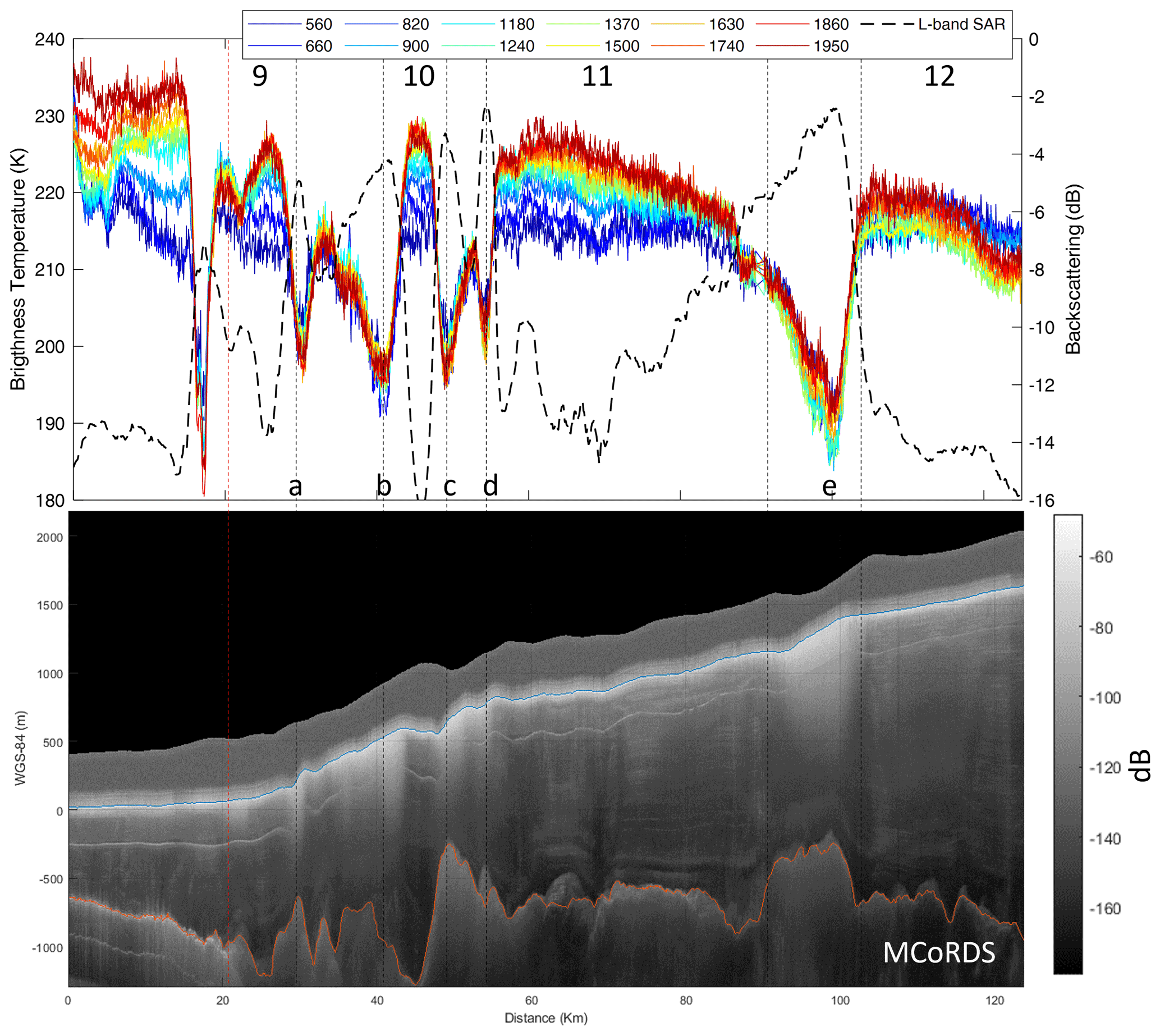
Figure 12 Comparison between UWBRAD data collected over Priestley Glacier (upper panel) and MCoRDS acquisitions (lower panel, color scale indicates the intensity of the MCoRDS radargram). The continuous blue line indicates the surface of the glacier, while the glacier bedrock is marked in red. The vertical dashed red line marks the glacier grounding line.

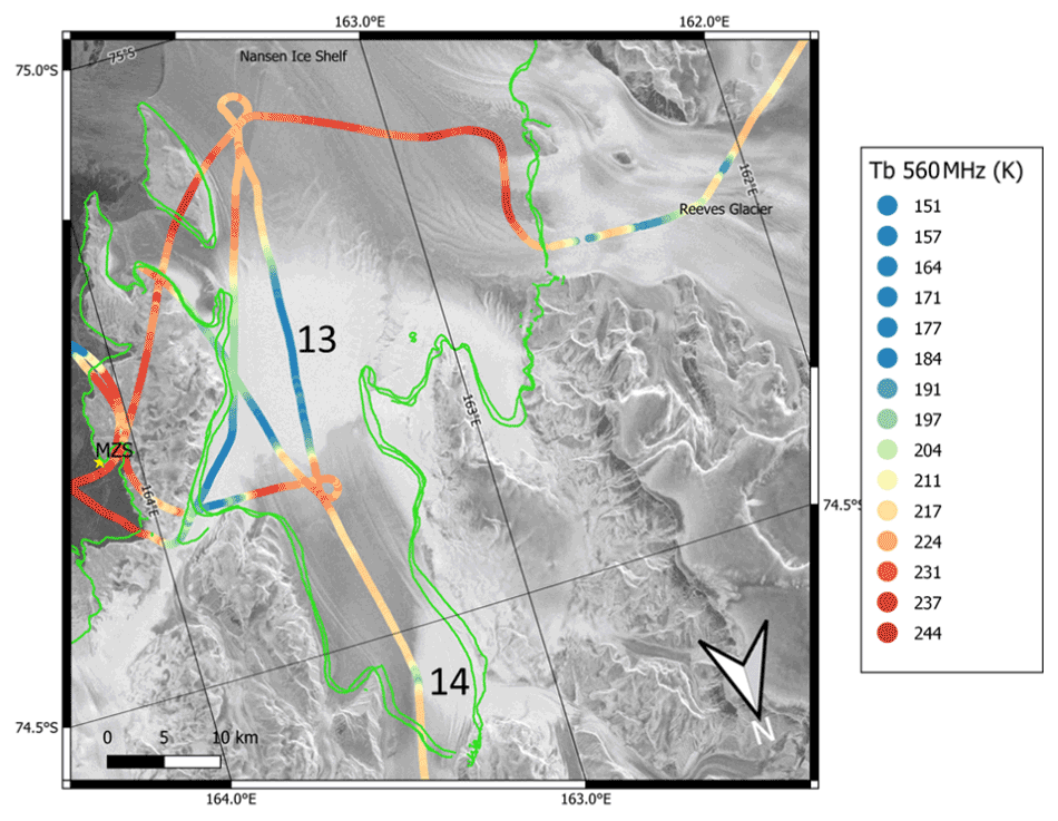
Figure 13 Map of transects over the Nansen Ice Shelf. The color scale indicates the 560 MHz brightness temperature, while the background image is C-band SAR data acquired by Sentinel-1 in November 2018. The green curves indicate the grounding line as derived from MEASURES dataset, while sites 13 and 14 are snow accumulation areas described in the text.

5.3 Nansen Ice Shelf

UWBRAD measurements were also performed over the Nansen Ice Shelf (which is fed by the Priestley and Reeves Glaciers). Due to katabatic winds that hampered the flight, only the northern portion was surveyed. The 560 MHz brightness temperatures shown in Fig. 13 point out a variety of features in this region. For example, in the final section of the Reeves Glacier, just upstream from the grounding line, 560 MHz brightness temperatures show strong variations, with minima around 170 K over crevassed areas and maxima around 230 K over more compacted ice regions. These values are in line with those measured over the Priestley Glacier (Fig.12). The 560 MHz brightness temperatures over the ice shelf are in contrast quite high, in the range 220–240 K. Additional variations are noted on the path from Reeves Glacier to Inexpressible Island that appear highly correlated to the C-band backscattering variation of the Sentinel 1 background image.

UWBRAD brightness temperatures for site 13 are compared in Fig. 14 with L-, C- and X-band SAR measurements and the GPR-measured radargrams. The Sentinel-1 SAR image indicates the presence of a snow accumulation region at site 13 at the end of the Priestley Canyon (ALOS and COSMO-SkyMed images have a similar pattern, which is not shown here). Before and after the snow zone, brightness temperatures are quite high, on the order of 225 K for all channels, and drop to values ranging from ∼ 185 K (560 MHz) to ∼ 145 K (1950 MHz) in the snow-covered area. This behavior is inversely correlated with the SAR backscattering variations, which show higher backscatter over the snow and lower backscatter over the blue ice region. At UWBRAD frequencies, dry snow is expected to be transparent, with the dominant effect being the weak multiple reflections between layers of different density (e.g., Brogioni et al., 2015). The snow zone encountered here appears to represent a high-scattering layer of maximum 20 m thickness (estimated from MCoRDS, in GPR data the depth of scattering area exceeds the investigation range which is about 12 m) buried below a 1 m layer of non-scattering snow. The most reasonable explanation for this behavior is the seasonal melt–refreeze cycles of the snow in which liquid water percolates into the snowpack to form larger ice lenses and/or columnar ice inclusions that cause increased scattering. Given that the snow area is not eroded by the winds, the inclusions have grown sufficiently large to cause scattering at these low frequencies.

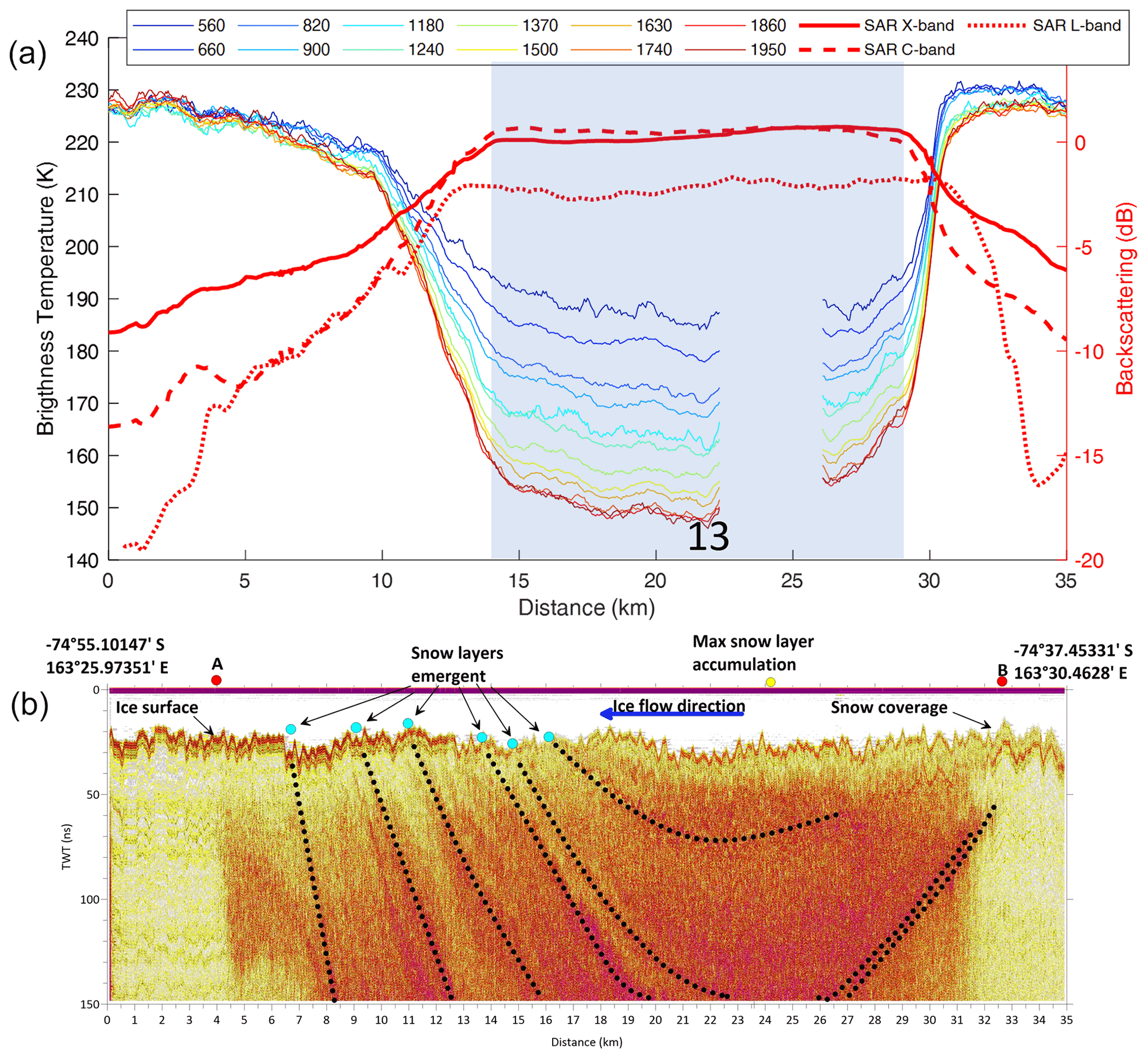
Figure 14 Comparison between UWBRAD and SAR data collected across the snow zone on the Nansen Ice Shelf (a) and GPR acquisitions (b). The red color scale indicates the intensity of GPR radargram. The shaded area indicates data collected over site 13. Data missing around the 25 km mark was caused by a strong electromagnetic interference.

This behavior is similar to that observed by Jezek et al. (2017) in the percolation zone inland of Nunatarsuaq, Greenland. Note that lower frequencies are expected to be less affected by scattering than higher frequencies, as observed in the measured brightness temperature time series in Fig. 14. Air temperature measurements collected by the AWS Sofia (74.8167^∘ S, 163.2333^∘ E, very close to the snow area) over the period 1987–2002 show that air temperatures rose above 0 ^∘C for several days almost every year. A similar analysis of data from AWS Zoraida (74.16^∘ S, 162.7392^∘ E, located 40 km upstream of site 13 at an elevation of 880 m m.s.l. – about 800 m higher), showed that the air temperature rose above 0 ^∘C at least three times in the last 30 years. An analysis of the melt presence indicator (Torinesi et al., 2003) applied to the K-band brightness temperatures from Advanced Microwave Scanning Radiometer 2 (AMSR2, Japan Aerospace Exploration Agency, 2013) confirms that seasonal melt can occur in some years in this region, meaning that the presence of larger scatterers is plausible.

A similar behavior is noted also at the confluence between the O'Kane and Priestley glaciers at site 14 (Fig. 13), where GPR measurements again show a higher scattering layer beneath an upper snow accumulation layer. This effect could again be explained by the melt–refreeze of snow accumulated by turbulence of the katabatic winds in the final bend of Priestley canyon.

5.4 Rocks

Exposed rocks are another interesting target for UWBRAD since they represent one of the “hottest” brightness temperature objects observed. In Terra Nova Bay, “rocks” consist mainly of granite and volcanic layers that appear dark in optical imagery. During flight 2, two sites were surveyed that were sufficiently large to cover a UWBRAD footprint: a nunatak in the David Glacier region (75.47340^∘ S, 159.60^∘ E, 1315 m a.s.l.) and a portion of Inexpressible Island (74.8780^∘ S, 163.6408^∘ E, 258 m a.s.l.). Surface temperatures derived from Landsat 8 for these locations were −15 and −9 ^∘C, respectively, which is consistent with a moist adiabatic lapse rate of about 5 ^∘C km⁻¹ (Krinner and Genthon, 1999; Minder et al., 2010). The spectra collected over these sites (Fig. 15) show average values of 234.6 K for the nunatak and 240.6 K for Inexpressible Island, in line with their physical temperature, with variations within ±2 K. The microwave emissivity estimated for both sites is then 0.91. The similarity of these results to the ∼ 237 K brightness temperature observed for the coastal moraine (centered at 74.730865^∘ S, 164.001^∘ E) is also suggestive of similar terrain properties in these regions.

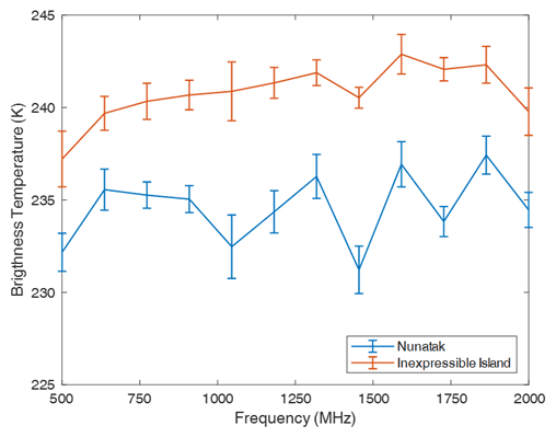
Figure 15 Brightness temperature spectra over a nunatak in the David Glacier region and over Inexpressible Island. Error bars indicate the range of brightness temperatures observed during the overpass.

5.5 Supraglacial lakes

The ability of 500–2000 MHz radiometry to probe the ice subsurface is particularly intriguing for the detection of internal aquifers. A UWBRAD transit over the Northern Foothills from Tethys Bay to the open sea acquired data over several targets including Enigma Lake, a supraglacial lake usually buried by an ice layer whose thickness varies from a few centimeters to about 15 m. The corresponding brightness temperature time series in Fig. 16 begins over the thick ice of Tethys Bay, then passes over the Strandline Glacier (a small glacier of ∼ 20 m thickness) before observing Enigma Lake followed by Boulder Clay Glacier (a glacier whose thickness reaches a maximum of 120 m) and open-sea observations. Brightness temperature spectra from the Boulder Clay and Strandline glaciers shown in Fig. 16b decrease with frequency at a rate that apparently depends on the morphological characteristics of the ice (thickness, accumulation, bedrock, etc.). The ice core moraine calibration region is composed by debris of granite and volcanic rocks of about 1 m thickness and shows values near the enforced flat spectrum. The spectrum from Enigma Lake shows an increasing trend similar to that for open water but much warmer (from 190 to 210 K). These distinct signatures for glaciers and the supraglacial lake highlight the potential of ultrawideband radiometry to detect aquifers and other subsurface hydrological features.

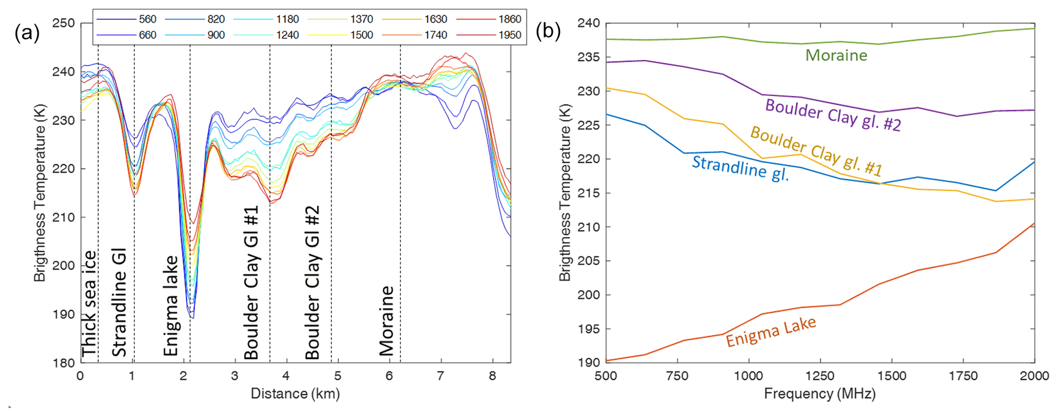
Figure 16 (a) Time series of brightness temperature acquired over the Northern Foothills and (b) spectra of the different targets imaged.

6 Conclusions

ISSIUMAX was the first campaign in Antarctica aimed at assessing the potential of low-frequency ultrawideband radiometry for cryospheric studies in coastal and inland areas. The distinct targets observed during the flights (sea ice, landfast sea ice, ice shelf, land ice) and the results highlight the benefits of using UWBRAD-like instruments for (i) discriminating between different glacier and sea ice regimes, (ii) making use of frequencies lower than 1.4 GHz to probe the volume of the targets, and (iii) measuring of a wideband spectrum that allows for probing different parts of the scene simultaneously. Together these observational characteristics offer a better capability to discriminate surface and/or subsurface properties, including the presence of snow on sea ice or ice shelves and the presence of liquid marine water in an ice shelf or brine in sea ice. The principal aim of the campaign was to test the new technique over as many targets as possible in order to assess its potential for cryospheric studies. Although in situ data were limited for most of the targets, valuable qualitative conclusions were nevertheless achieved, as detailed for each target type in what follows.

The sea ice surveyed in the campaign can be divided into two classes: very thick fast ice (>2 m) and shallow young ice (<50 cm). As expected from theoretical computations (Jezek et al., 2019; Demir et al., 2022a), this implies that the brightness temperature spectrum measured was in the first case flat with very high values (240–250 K) and in the second case similar to the values of open water (100–150 K). While we expect that the main benefit of using the entire 0.5–2 GHz band for sea ice is the retrieval of thickness within the 0.5–1.5 m range (Macelloni et al., 2018), the availability of low frequencies (<1 GHz) and T_b spectra were shown to improve sea ice type classification with respect to available present capabilities. For example, Fig. 6b shows that frequencies above 1.25 GHz provide similar information (i.e., the brightness temperature spectrum is flat above this frequency), while lower frequencies retain sensitivity to distinct ice properties. In addition, the availability of multispectral data with respect to a single L-band channel makes the sensing of properties such as water infiltration (site 8 in Fig. 8) or the presence of snow on top of the ice (sites 1 and 3 in Fig. 6, given that the presence of snow impacts lower frequencies more significantly than higher ones) possible. While the first result is motivated by the increased penetration depth of lower frequencies, the second is related to the effect of impedance mismatches (due to the presence of snow), which are more relevant to the lower frequencies. Lastly, data collected on thin sea ice (Fig. 10b) demonstrated a sensitivity to ice thickness that increases at low frequencies consistent with the predictions of an electromagnetic model. Although the thickness used as a reference is subject to error (because it was derived from TIR satellite data), the results suggest that while higher frequencies saturate at 20–50 cm thickness (depending on salinity), lower frequencies retain sensitivity to higher thickness values. The comparison of data collected over thin and thick ice also shows the importance of ice salinity in the electromagnetic emission. Sea ice 20 cm thick with a high brine content (e.g., salinity 12–15 g kg⁻¹) can have the same spectral signature as FYI 2 m thick (salinity 7 g kg⁻¹), underscoring the importance of ice salinity information in the thickness retrieval process.

The brightness temperatures collected over glaciers also show the importance of spectral measurements. Over the Priestley Glacier, the spectral slopes of brightness temperatures are sensitive to the disappearance of the first ∼ 100 m of firn due to wind erosion (sites 11 and 12 in Fig. 12). At site 11 the target is mainly composed of compacted thick ice, and the spectrum slope is positive (up to 5 K GHz⁻¹), while at site 12 the spectrum is more similar to those in the inner part of the ice sheet with a negative slope of −4 K GHz⁻¹ (Brogioni et al., 2022). Figure 12 shows distinct spectral features outside the crevasse zones (sites 9, 10 and 11). A deeper analysis of this behavior would require a detailed analysis that includes additional information on the glacier structure that is beyond the scope of this paper, including consideration of the ice temperature profile and potential impacts of volume scattering. It is also interesting to note the different spectral behavior before and after the grounding line (e.g., 25 km and 15 km in Fig. 12): brightness temperatures decrease at lower frequencies but increase at higher frequencies. This can be due to the change of the bottom medium (bedrock to seawater) and the structure of the ice at the hinge point. Crevassed areas are characterized by a marked drop in brightness temperature at all frequencies resulting in a flat spectrum (sites a–e in Fig. 12). It is also noted that the same behavior is observed over the Reeves Glacier (blue and orange fluctuations in Fig. 13) and David Glacier (orange fluctuations in Fig. 4), although the relative time series are not shown here.

The Nansen Ice Shelf was surveyed only in its northern region. Although clear changes in the brightness temperature signal were noted while transiting from the Reeves Glacier to Inexpressible Island, the snow accumulation zone at the end of the Priestley Canyon (site 13 in Fig. 13) showed particularly distinct impacts. Before and after the snow area, over blue ice, the spectrum is flat (as observed for crevassed areas of glaciers or for very thick ice) with a value of about 230 K (Fig. 14-top). As the aircraft transited over snow, the T_b decreased to an extent that was greater at higher than at lower frequencies. This is in agreement with electromagnetic scattering theory and suggests the presence of ice lenses and columnar ice not ablated by the katabatic winds. GPR measurements also support this finding.

Heterogeneous areas with different targets including buried supraglacial lakes were also observed. While transiting from Tethys Bay to Adelie Cove through the Northern Foothills, data were collected over several different scenarios: fast ice, supraglacial lake, glacier and moraine. As shown in Fig. 16, brightness temperatures show fluctuations at all frequencies, but spectral information nevertheless clearly distinguishes these different targets. While the moraine shows a flat spectrum (i.e., the permittivity of rock is almost constant in frequency), snow-covered glaciers have a decreasing spectral trend, as seen for the Campbell Glacier Tongue (Fig. 6) and the ice sheet (Andrews et al., 2018; Brogioni et al., 2022). Also, Enigma Lake shows an increasing spectral trend that is similar to spectra observed for open water but with a higher brightness temperature level due to the emission of the overlying ice. It is also noted that although sea ice and subsurface water both show an increasing spectral trend, sea ice usually shows a saturation (e.g., young ice spectra in Fig. 10b), while the subsurface water spectra show a steadily increasing trend. If needed, this different behavior can used as a discriminator between these two target types.

The campaign also showed that brightness temperature data were observable over the entire 0.5–2 GHz range in Antarctica after appropriate RFI processing, despite the heavy use of this frequency range by other services in more populated areas.

Overall, the ISSIUMAX campaign has demonstrated the capabilities of ultrawideband airborne radiometry for studying near-coastal ice sheets that represent a transfer zone between the inland ice sheet and the ocean. The use of brightness temperature spectrum over a wide band allows the discrimination of surface and subsurface characteristics well beyond the current capabilities of existing L-band radiometers. It is noted that some of the interesting features observed within the flights occur at spatial scales too small to be resolvable from current or planned spaceborne systems so that only airborne data can be suitable for their monitoring. For example, the width of the outlet glaciers overflown is too small to separate contributions from the ice and from the rocky walls. Nevertheless, the general properties of the different targets observed (e.g., the presence of snow on top of sea ice and ice shelves; the classification of surface types; sea ice thickness) can nevertheless be expected to be observable from space and can contribute to better monitoring of key glaciological parameters and their evolution. The campaign also showed that further investigations and dedicated experiments that include more extensive in situ data collection are needed to better understand the complex mechanisms that govern the microwave emission at these frequencies and to extend current electromagnetic models.

Appendix A: UWBRAD calibration and RFI processes

The UWBRAD radiometer includes an internal calibration process that cycles through measurements of the “antenna”, “antenna plus noise diode”, “reference load” and “reference load plus noise diode” states every 2 s. Each measurement corresponds to a 100 ms observation and includes the “fullband” power in each 88 MHz sub-channel at 1 ms time resolution, the “sub-band” power in 512 frequency sub-channels within the 88 MHz sub-channel at 1 ms time resolution (called the power spectrogram in what follows), the kurtosis of the fullband power reported at 1 ms time resolution and the kurtosis in each frequency sub-band at 100 ms time resolution. RFI detection is performed through a combination of algorithms including detectors using the fullband and sub-band kurtosis quantities, as well as searches for anomalous results in both time and frequency. Additional information on these algorithms and on the RFI encountered is provided in Andrews et al. (2021). Note that the exclusion of pixels from subsequent integrations degrades the sensitivity of the integrated product. It has been estimated that the loss of up to 75 % of the data for an acquisition will cause the noise equivalent delta temperature (NEdT) to double from 0.5 to 1 K in that specific channel. However, sensitivity can be regained following integration over multiple measurements within the 4.5 s (or longer with degraded spatial resolution) integration time available. A detailed assessment of the RFI impact on the UWBRAD measurements was performed by Andrews et al. (2021) by using experimental data collected in both polar regions. As expected, RFI have a strong impact on data acquisition over areas having higher human presence (e.g., Canada) but lesser (Greenland) to negligible (Antarctica) in remote regions. In Greenland the loss of the 75 % of the acquisitions happened less than the 10 % of the time and only for a few specific channels.

The internal calibration process described in Andrews et al. (2018) is used to compensate for the impact of changes in system temperature or receiver gains on measured data. Internally calibrated measurements are then used to create absolute calibrated brightness temperatures through an external calibration process that uses observations over the open sea surface and over the coastal moraine region, for which model predictions of the expected brightness temperatures as a function of frequency were applied. Sea surface brightness temperatures were predicted using a two-scale model (Johnson, 2006) applied with wind speed and sea surface temperature information from the European Center for Medium Range Weather Forecasting (ECMWF). An approximate correction for the reflection of cosmic and atmospheric emission was also included in the sea brightness temperature model prediction. The coastal moraine area (−74.745^∘ S, 164.0271^∘ E) was modeled as having a spectrally uniform brightness temperature of 237 K, which would correspond to a homogeneous interface having a relative permittivity of ∼ 4.5 at the estimated 272 K physical temperature at this location known from an automated weather station (AWS) at this site. This value for the moraine area was assigned based on extensive studies showing the apparent spectral flatness of the observed data at this location as well as the known properties of the terrain in the area. The external calibration process enforces a match to these predictions and agreement in “cross-over” measurements through a least-squares process that determined the gain and offset parameters in a linear rescaling of the internally calibrated data. The external calibration process was applied first at the level of the $\mathrm{12}\times \mathrm{512}=\mathrm{6144}$ individual spectral channels available following initial RFI processing, with additional RFI processing performed after external calibration. The least-squares external calibration algorithm was again applied to the 12 frequency channels obtained after integrating the data over the 512 frequency sub-channels in each channel, and additional RFI processing was also performed following this combination. An additional step in the external calibration and RFI filtering process as compared to Andrews et al. (2018) enforces the “spectral smoothness” of the observed data at both the 6144 and 12 channel levels as previously developed in (Gasiewski et al., 2002). The algorithm performs a fourth-order polynomial fit to the measured data versus frequency and flags outliers from the fit through an iterative process in which the detected outliers are first excluded, a new fit is determined to the remaining data, adjustments to the calibration coefficients of the excluded channels (for an entire flight) are made based on the current fit in order to attempt to retain these channels, and the process is repeated including the adjusted sub-channels and using a refined detection threshold. Following this process, any sub-channels showing excessive errors in matching the prescribed brightness temperature values for the sea and moraine calibration targets are ultimately discarded. This approach was required due to the challenges of estimating ultrawideband brightness temperatures given the effects of impedance mismatch and the presence of RFI that varies in space and time.

Appendix B: ISSIUMAX dataset

Here a list of the Earth observation (EO) product datasets used for planning the ISSIUMAX campaign and the supporting UWBRAD data interpretation is provided. The product list is not limited to the ones used in the present paper but covers the entire campaign given that large parts of the UWBRAD dataset are still to be analyzed in depth by the team in the framework of new projects and collaborations:

• 70 SAR SCS 1B products from COSMO-SkyMed® (X-band), 20–27 November 2018, acquired in Stripmap Himage mode, HH polarization, 3 m ground resolution;

• 118 SAR GRD products from Sentinel-1 (C-band), from 7 January to 30 November 2018, HH pol, 10 ground resolution;

• 96 SAR GRD products from ALOS-PALSAR (L-band), from 7 October 2007 to 20 January 2011, HH pol, 5 m ground resolution;

• SMOS (Kerr et al., 2010) and SMAP (Piepmeier et al., 2016) L-band brightness temperature images for intercalibration with UWBRAD;

• T_b data from JAXA's AMSR-2 at C to Ka band to better constrain the inversion algorithms;

• Sentinel-2 optical images acquired on 22 November 2018 and 2 January 2019;

• Landsat-8 optical images collected on 24 and 27 November 2018;

• ICESaT-2 measurements ATL-7 (https://doi.org/10.5067/189WL8W8WRH8) and ATL-10 (https://doi.org/10.5067/189WL8W8WRH8) acquired on 23 and 27 November 2018;

• medium-resolution images from Sentinel-3 and MODIS for monitoring sea ice presence and movements from NASA's EOSDIS Worldview app (https://worldview.earthdata.nasa.gov/, last access: 12 January 2023);

• Accumulation Radar (Paden et al., 2014) and MCoRDS (Paden et al., 2010) data collected during 2013 Operation Ice Bridge campaign on 19–20 November 2013;

• high-resolution nadir L-band T_b over Dome C obtained from the past DOMECair campaign (Domecair dataset, 2013);

• ground-based L-band brightness temperatures from the DOMEX experiment used as a reference in UWBRAD calibration (Domex-3 dataset, 2017).