the Creative Commons Attribution 4.0 License.
the Creative Commons Attribution 4.0 License.
 | 02 Jun 2023
Wind redistribution of snow impacts the Ka- and Ku-band radar signatures of Arctic sea ice
Rosemary Willatt
Robbie Mallett
Julienne Stroeve
Torsten Geldsetzer
Randall Scharien
Rasmus Tonboe
John Yackel
Jack Landy
David Clemens-Sewall
Arttu Jutila
David N. Wagner
Daniela Krampe
Marcus Huntemann
Mallik Mahmud
David Jensen
Thomas Newman
Stefan Hendricks
Gunnar Spreen
Amy Macfarlane
Martin Schneebeli
James Mead
Robert Ricker
Michael Gallagher
Claude Duguay
Ian Raphael
Chris Polashenski
Michel Tsamados
Ilkka Matero
Mario Hoppmann
Wind-driven redistribution of snow on sea ice alters its topography and microstructure, yet the impact of these processes on radar signatures is poorly understood. Here, we examine the effects of snow redistribution over Arctic sea ice on radar waveforms and backscatter signatures obtained from a surface-based, fully polarimetric Ka- and Ku-band radar at incidence angles between 0∘ (nadir) and 50∘. Two wind events in November 2019 during the Multidisciplinary drifting Observatory for the Study of Arctic Climate (MOSAiC) expedition are evaluated. During both events, changes in Ka- and Ku-band radar waveforms and backscatter coefficients at nadir are observed, coincident with surface topography changes measured by a terrestrial laser scanner. At both frequencies, redistribution caused snow densification at the surface and the uppermost layers, increasing the scattering at the air–snow interface at nadir and its prevalence as the dominant radar scattering surface. The waveform data also detected the presence of previous air–snow interfaces, buried beneath newly deposited snow. The additional scattering from previous air–snow interfaces could therefore affect the range retrieved from Ka- and Ku-band satellite altimeters. With increasing incidence angles, the relative scattering contribution of the air–snow interface decreases, and the snow–sea ice interface scattering increases. Relative to pre-wind event conditions, azimuthally averaged backscatter at nadir during the wind events increases by up to 8 dB (Ka-band) and 5 dB (Ku-band). Results show substantial backscatter variability within the scan area at all incidence angles and polarizations, in response to increasing wind speed and changes in wind direction. Our results show that snow redistribution and wind compaction need to be accounted for to interpret airborne and satellite radar measurements of snow-covered sea ice.
- Article
(7036 KB) - Full-text XML
- BibTeX
- EndNote


Wind plays an important role in shaping the spatial distribution of snow depth and snow water equivalent (SWE) over sea ice (Moon et al., 2019; Iacozza and Barber, 2010). Wind alters snow temperature gradients through wind pumping (Colbeck, 1989), structural anisotropy (Leinss et al., 2014), and snow grain geometry (Löwe et al., 2007). Furthermore, wind affects the residence and sintering time of snow close to the surface, facilitating depositional snow dune growth and erosional processes (Trujillo et al., 2016). Fluctuating wind speed and direction modify snow surface topography and density via wind scouring and compaction of snow (Lacroix et al., 2009). Depending on the ice surface roughness (e.g., level ice, pressure ridges, hummocks etc.), wind will result in the formation of heterogeneities at different scales, from ripple marks to snow bedforms and drifts (Filhol and Sturm, 2015). This further alters the geometric-, aerodynamic-, and radar-scale roughness (Savelyev et al., 2006).
Under cold snow conditions, a common assumption in radar altimetry is that the dominant scattering surfaces of co-polarized Ka- and Ku-band radar signals correspond to the air–snow and snow–sea ice interfaces, respectively (e.g., Armitage et al., 2015; Tilling et al., 2018). For synthetic aperture radar (SAR) and scatterometry, variations in snow grain microstructure influence the proportion of surface and volume scattering to the total radar backscatter (Nandan et al., 2017). Winds can roughen or smoothen the snow surface on relatively short timescales, altering the Ka- and Ku-band surface and/or volume scattering contributions to total radar backscatter.
Very little is known about how wind redistribution of snow impacts snow depth, SWE, and ice thickness retrievals from airborne and satellite radars (Yackel and Barber, 2007; Kurtz and Farrell, 2011). Due to repeat airborne and satellite ground tracks often occurring weeks/months apart and sea ice drift, it is challenging to measure radar backscatter changes resulting from wind redistribution on the same area of ice over time. Nevertheless, Kurtz and Farrell (2011) assumed snow redistribution caused an anomalous snow depth decrease in 2009 over multi-year sea ice in the Canadian Archipelago (CA), retrieved from two Operation IceBridge (OIB) snow radar flights, acquired 3 weeks apart. Yackel and Barber (2007) speculated that snow redistribution on first-year sea ice in the CA was, in part, responsible for a change in retrieved SWE of up to 7 cm, derived from two C-band RADARSAT-1 images 45 d apart.
To better understand the impact of snow redistribution on Ka- and Ku-band radar signatures, we require unambiguous in situ measurements of snow physical properties and meteorological observations during wind events, sampled coincidentally with radar measurements. This bridges a fundamental knowledge gap and potentially allows improved modeling of Ka- and Ku-band radar waveforms and backscatter. This in turn may improve interpretation of Ka- and Ku-band radar signatures from presently operational SARAL/AltiKa (Guerreiro et al., 2016), CryoSat-2 (Lawrence et al., 2018), Sentinel-3 (Lawrence et al., 2021), ScatSat-1 (Singh and Singh, 2020), and the upcoming Ka-/Ku-band CRISTAL altimetry (Kern et al., 2020) and SWOT satellite missions (Armitage and Kwok, 2021).
In this study, we investigate wind-induced changes to snow physical properties and topography on Ka- and Ku-band radar signatures, including dominant scattering surfaces and backscatter, using a surface-based, fully polarimetric Ku- and Ka-band radar (KuKa radar; see Stroeve et al., 2020) deployed during the 2019–2020 Multidisciplinary drifting Observatory for the Study of Arctic Climate (MOSAiC) expedition (Nicolaus et al., 2022). We present data from 9 to 16 November 2019, assessing the effects of two separate wind events (WE1 and WE2). First, we describe the KuKa radar system, the time series of meteorological observations, snow physical properties, and snow surface topography. Next, we investigate the impact of snow redistribution on KuKa radar echograms and waveforms, examining changes in dominant scattering surfaces and radar backscatter. Finally, we discuss the relevance of our findings to improving retrievals of snow–sea ice geophysical variables by airborne and satellite radars.
2.1 Surface-based Ka- and Ku-band polarimetric radar (KuKa radar)
During the MOSAiC expedition, the research icebreaker R/V Polarstern drifted with a sea ice floe across the central Arctic Ocean over a full annual cycle (Nicolaus et al., 2022). The floe was dominated by second-year ice with refrozen melt ponds making up ∼ 60 % of the surface area. The remote sensing site (RSS) was first established on the floe on 18 October 2019, where the KuKa radar was deployed on ∼ 80 cm thick, laterally homogeneous, and undeformed sea ice.
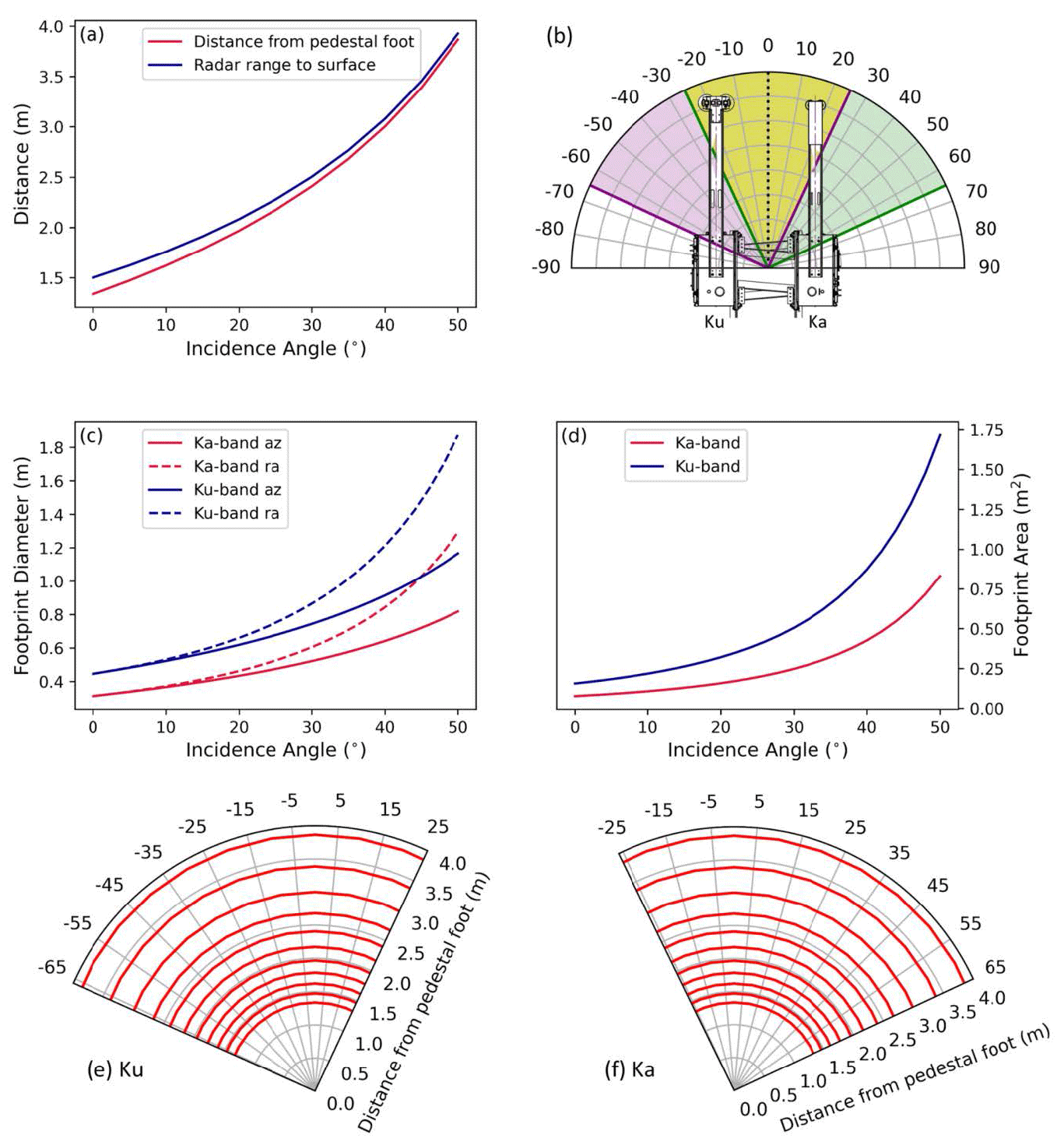
Figure 1KuKa radar geometry illustrating (a) radial distance and radar range from the pedestal foot; (b) KuKa radar azimuth scan pattern projected based on the positioner axis coordinate system (b) scan pattern of radar projected onto a level surface; (c) diameter of radar scan area, measured radially (ra) and azimuthally (az); (d) area of radar scan area; (e) and (f) Ku- and Ka-band scan area of the KuKa radar, respectively. In panel (b), the region between purple and green lines is the respective Ku- and Ka-band scan area (separately illustrated in panels (e) and (f)), while the yellow region in (b) is the overlapping scan area.
The KuKa radar transmits at Ka- (30–40 GHz) and Ku-band (12–18 GHz) frequencies and measures the return radar power (in dB) as a function of range (Stroeve et al., 2020). The radar acquires data across a fixed azimuth (θaz) range at discrete incidence angle (θinc) intervals. The radar operates in all vertical (V) and horizontal (H) linear polarization transmit and receive combinations: VV, HH, HV, and VH.
The central frequency of the radar chirps were set to be close to the Ka-band of AltiKa (35 GHz) and the Ku-band of CryoSat-2 (13.575 GHz). The KuKa radar bandwidth is considerably higher than the bandwidth of AltiKa and CryoSat-2, allowing for an improved range resolution of 1.5 cm for Ka-band and 2.5 cm for Ku-band relative to 30 and 46 cm for AltiKa and CryoSat-2, respectively. The radial distance and range from the pedestal, the scan area diameter, and scan area from θinc = 0–50∘ are illustrated in Fig. 1. During MOSAiC, the KuKa radar scanned over a 90∘ continuous θaz range width for every 5∘ interval in θinc. The KuKa radar takes ∼ 16 s (i.e., 5.7∘ per second) over a 90∘ θaz width to acquire data across an incidence angle scan line and ∼ 2.5 min for one complete scan between θinc = 0–50∘. There is a ∼ 20∘ offset between the individual radar antennas and the radar positioner axis origin. Therefore, the Ku-band antenna scans between the −65 and +25∘ θaz range (region between purple lines) and between −25 and +65∘ for the Ka-band (region between green lines) (Fig. 1b, e, and f). This also means that the Ku- and Ka-band scan area overlap for a given radar “shot” is θinc dependent. The yellow region between the green and purple lines in Fig. 1b between −25 and +25∘ is the overlapping Ku- and Ka-band scan area. The antenna beamwidth (6 dB two-way) is 16.9 and 11.9∘ for Ku- and Ka-bands, respectively. Therefore, the size of the radar scan area on the snow is dependent on frequency, the height of the antenna above the snow surface, and θinc. Further description of the radar specifications, signal processing, polarimetric calibration routine, signal-to-noise and error estimation is documented in Stroeve et al. (2020).
At the RSS, the radar acquired scans every 30 min over the 90∘ θaz width and θinc discrete increments. Between 9 and 15 November, a total of 325 scans were collected. The ice supporting the RSS broke up on 16 November, and the measurements were stopped until it was safe to redeploy the radar.
2.2 Meteorological and snow property data
A 10 m tall meteorological station installed ∼ 100 m away from the RSS monitored air temperature (∘C), relative humidity (%), air pressure (hPa), wind speed (m s−1), and wind direction (∘), all at 2 m height. Wind direction is denoted with respect to geographic north (0∘). Measurements were acquired every second (Cox et al., 2021) and resampled to 30 min averages to match the radar scan intervals.
A thermal infrared (TIR) camera (InfraTec VarioCAM HDx head 625, assuming emissivity 0.97 at 7.5–14 µm wavelength; Spreen et al., 2022) measured snow surface temperature (∘C) every 10 min. Two digital thermistor chains (DTCs) installed close to the RSS measured near-surface, snow, and sea ice temperature evolution at 2 cm vertical intervals. No destructive snow sampling was done underneath the KuKa radar scan area. Instead, snow depth measurements were made close to the radar on 4 and 14 November. Profiles of the penetration resistance force of the snow were collected before, during, and after WE1 and WE2 using a snow micro-penetrometer (SMP; Johnson and Schneebeli, 1999) at the Snow1, Snow2, and RSS sites (see locations in Fig. 4). Five SMP profiles per pit were recorded weekly. To compare initial density and specific surface area (SSA) between the RSS and the Snow1 and Snow2 locations at the beginning of November, one SMP profile from the RSS was taken on 4 November. The force profiles were converted into density and SSA following King et al. (2020) and Proksch et al.'s (2015) parameterizations, respectively, which also worked well during the MOSAiC winter (Wagner et al., 2022).
2.3 Snow surface topography
An optical camera was used to visualize snow surface topography changes within the radar scan area (Spreen et al., 2021). In addition, terrestrial laser scanning (TLS) data of snow surface topography were collected on 1, 8, and 15 November using a Riegl VZ-1000. Scan positions were registered in RiSCAN (Riegl's data processing software) using reflectors permanently frozen to the ice and leveled based on the VZ-1000's built-in inclination sensor. Wind-blown snow particles were removed from the data by FlakeOut filtering (Clemens-Sewall et al., 2022). Filtered data were aligned to one another by matching reflectors and other tie points. To transform the TLS data into the KuKa radar's reference frame, the outlines of the radar's pedestal column and the antenna arms were manually picked in the TLS data.
A non-linear least squares optimization method using SciPy (Virtanen et al., 2020) was then implemented to estimate the best-fitting circle and rectangle to match the pedestal column and the antenna arms, respectively. The center of the pedestal was used as the horizontal origin, the center of the antennas was used for orientation, and the antenna height at nadir position was used as the vertical origin. Within the radar's reference frame, a polar grid was defined with radial increments of 0.25 m and azimuthal increments of 10∘. The surface height in the radar reference frame (a.k.a. the vertical distance from the surface to the radar antennas at nadir) for each grid cell was calculated by averaging the vertical position of each TLS point within that grid cell.
2.4 Radar waveforms and backscatter
Waveforms from each sampling time across θaz were recorded and overlaid with the TLS data to identify where the Ka- and Ku-band backscatter originated from (Sect. 3.2). Deconvolved waveforms were used (Stroeve et al., 2020), using waveforms from refrozen lead located close to the RSS in January 2020 to provide a specular return useful for reducing the appearance of sidelobes that result from non-ideal behavior of the RF electronics, as well as internal reflections in the radar. Waveform echograms were used to illustrate how the return waveforms from within the overlapping scan area changed between WE1 and WE2. The normalized radar cross section per unit area (NRCS) was calculated based on the range–power profiles following the standard beam-limited radar range equation (Ulaby et al., 2014) given by
where h is the antenna height; RC is the range to the corner reflector; θ3dB is the one-way half-power beamwidth of the antenna; and and are the received power from the snow and the corner reflector, respectively.
The peak power in the radar waveforms used for calculating NRCS is determined by locating the highest peak in the waveform averaged across all polarizations. For waveform analysis, we calculated NRCS at nadir for the air–snow and snow–sea ice interfaces by integrating the power over the waveform peaks within ±2 dB on either side of the overlapping scan area (Sect. 3.2). Next, we calculated the NRCS value integrated over the entire snow volume based on the power contained within this peak over an incidence angle scan line by integrating over the range bins where the power falls below a threshold, set to −50 dB on either side of the peak for Ka-band data and −20 dB (−40 dB) on the smaller-range (larger-range) sides for Ku-band data. The NRCS was averaged across the overlapping scan area across the entire 90∘ θaz range, at discrete θinc=0, 15, 35, and 50∘, to demonstrate the scan-area-scale variability in backscatter during the two wind events (Sect. 3.3).
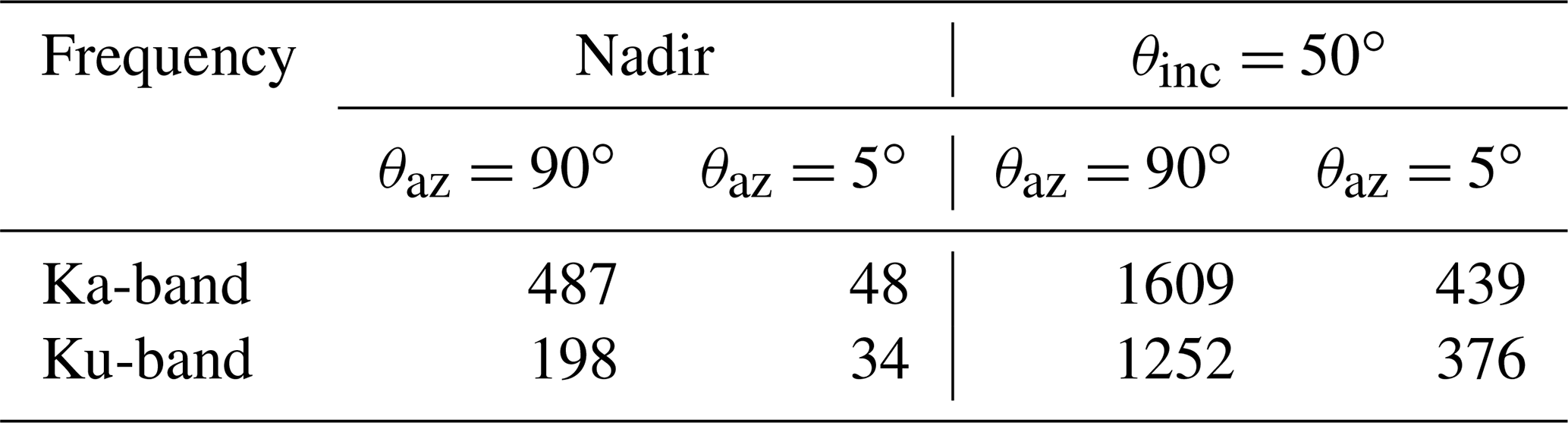
To investigate the backscatter variability within the scan area caused by surface heterogeneity, as well as the range to the dominant scattering surface that could have changed during sampling, we used azimuth “sectoring” and analyzed the NRCS averaged at 5∘ wide θaz bins. Azimuth sectoring has an impact on the number of independent samples in the range along a 5∘ θaz bin, since a smaller area is used for averaging (Table 1). The number of independent samples is estimated based on the following steps. (a) Determine the distance between the 6 dB points below the radar range peak on either side of the peak. (b) Divide the 6 dB range by the range resolution; this is a measure of the number of independent samples in range. (c) Divide the azimuth width (90 and 5∘ in our study) by the azimuth beamwidth and multiply by 2. (d) The total number of independent samples would then be the number of independent samples in range multiplied by the number of independent samples in azimuth (Doviak and Zrnić, 1993).
Table 1Number of independent samples at Ka- and Ku-band frequencies at nadir and θinc=50∘ at θaz=90∘ and along a 5∘ bin.
Within every θinc scan, VV, HH, and HV are derived from the complex covariance matrix, while VH is discarded based on reciprocity of cross-polarized channels (i.e., HV ∼ VH) (Ulaby et al., 2014). In Sect. 3.3.2, we show the changes in backscatter signature variability across the KuKa radar scan area at 5∘ wide θaz bins at specific times on 9, 11, and 15 November.
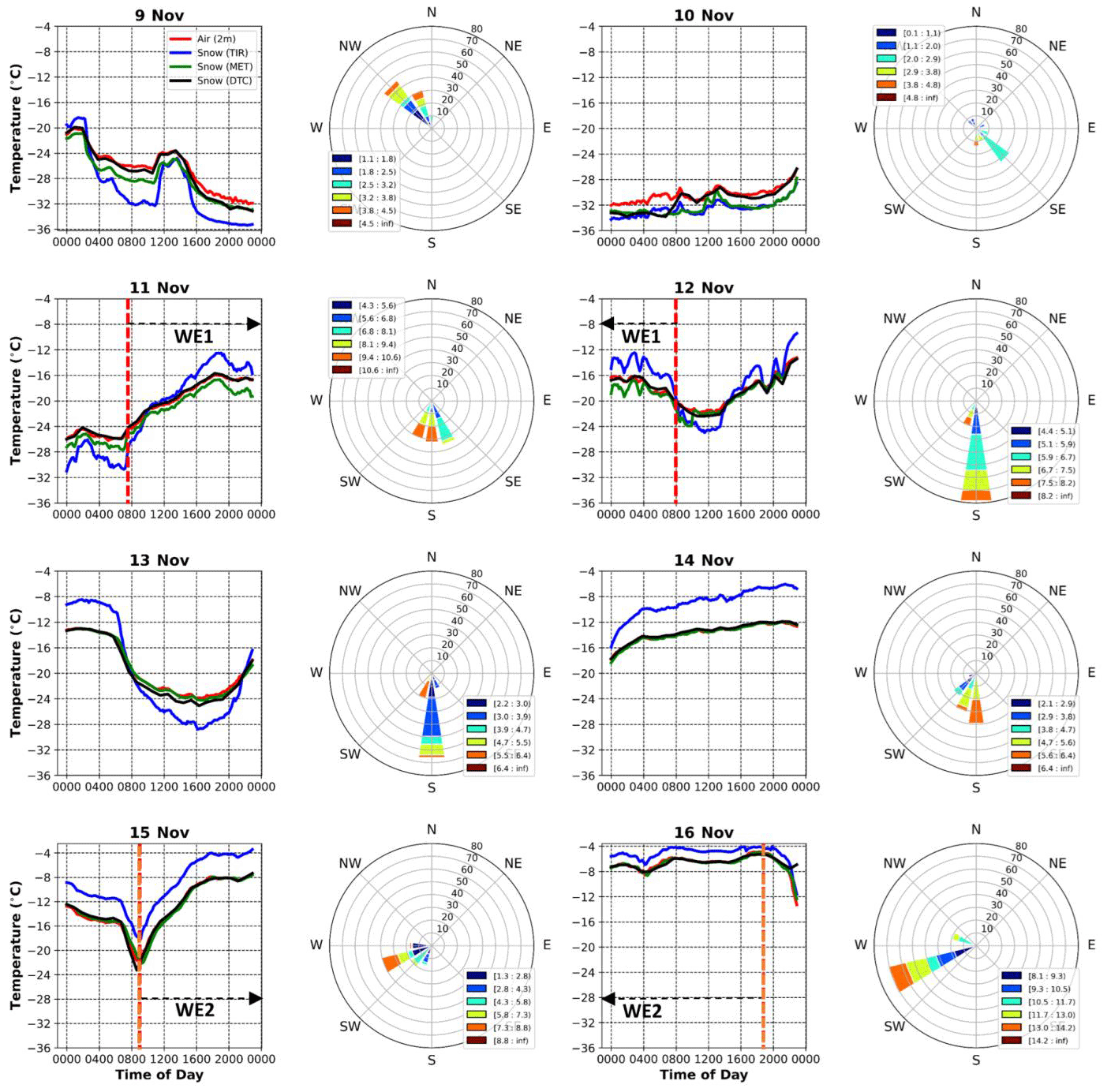
Figure 2Line plots illustrate daily, 30 min averages of 2 m air temperature (MET tower) and snow surface temperature measurements from the TIR camera, MET tower, and DTC sensors; measurements were acquired between 9 and 16 November. Wind rose plots illustrate corresponding wind speed (m s−1) and direction (∘) measurements recorded by the MET tower. All times are UTC. Dotted red and orange lines indicate the onset of WE1 and WE2, respectively, supported by black arrows.
3.1 Meteorological and snow conditions
3.1.1 WE1 and WE2
WE1 started ∼ 07:45 UTC on 11 November and lasted until ∼ 08:00 UTC on 12 November when winds ∼ 12 m s−1 originated from the SW to SE (Figs. 2 and 3c). WE2 started ∼ 09:00 UTC on 15 November, when a low-pressure system began to intensify (Fig. 3b). The wind direction shifted from SW to W, and speeds increased to ∼ 15 m s−1 and continued until ∼ 19:00 UTC on 16 November (Figs. 2 and 3c). During WE2, the strong low-pressure system dropped below 995 hPa (Fig. 3d), and the air temperature reached −5.5 ∘C (Fig. 3a). The warm air advection was accompanied by a steep increase in relative humidity to >90 % (Fig. 3d).
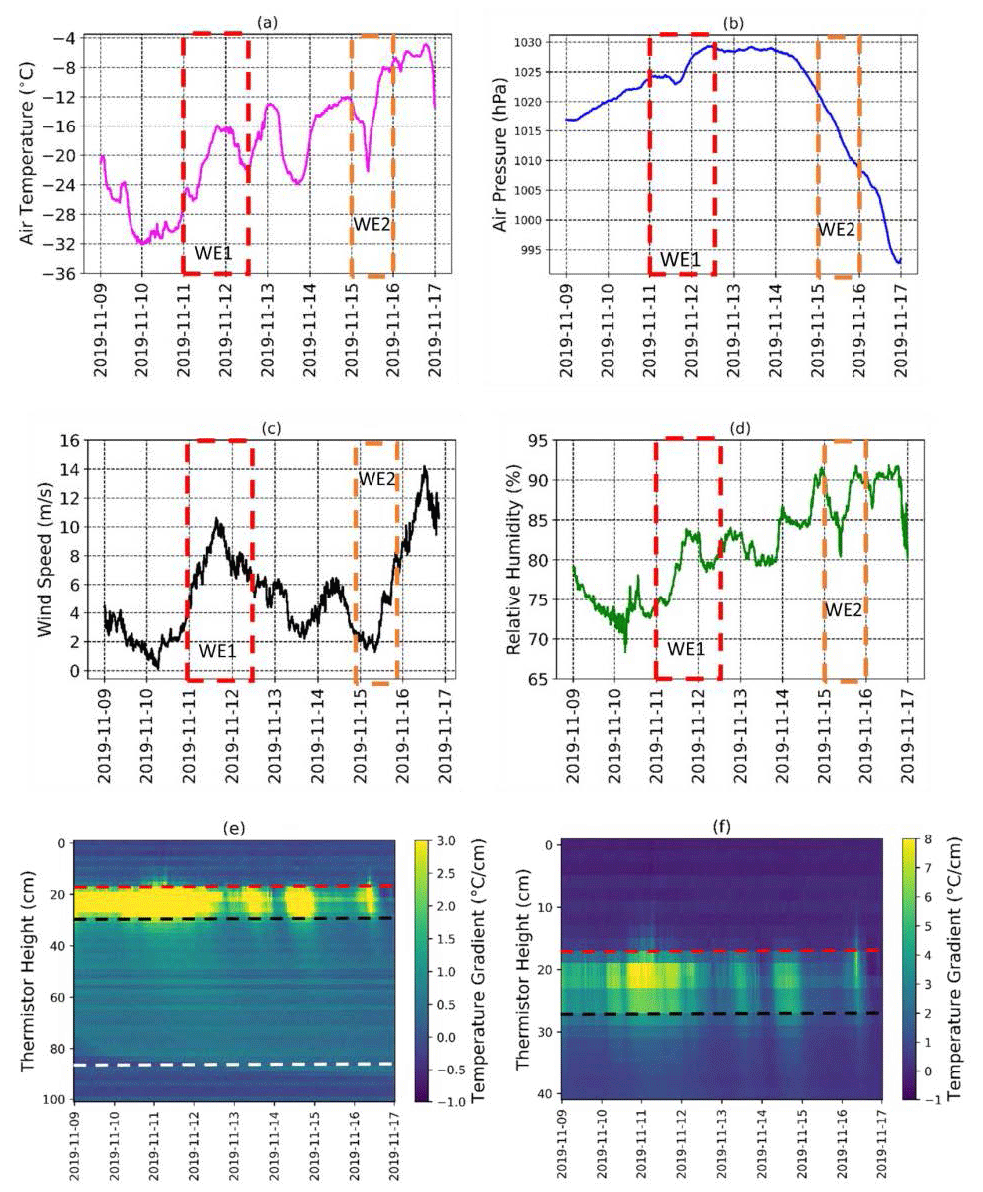
Figure 3Line plots show daily, 10 min averaged 2 m (a) air temperature, (b) air pressure, (c) wind speed, and (d) relative humidity recorded by the MET tower between 9 and 16 November. Two-dimensional color plots show DTC-derived hourly averaged temperature gradients of (e) near-surface, snow, sea ice, and ocean, and (f) the sub-section of panel (e) shows the snow volume from the RSS. Yellow represents larger temperature gradients within the snowpack. Dotted red, black, and white lines represent approximate locations of the estimated air–snow, snow–sea ice, and sea ice–ocean interfaces. DTC temperature sensors are spaced by 2 cm, with the top 20 cm representing the height above the air–snow interface. Red and orange boxes in (a) to (d) indicate WE1 and WE2 windows. Note the different temperature gradient scales for (e) and (f).
3.1.2 Snow temperature, density, and microstructure
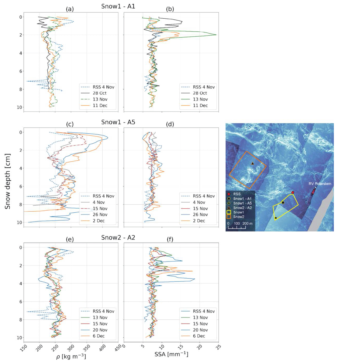
Figure 4The upper 10 cm of the horizontally averaged density and SSA profiles of the snowpack over time derived from the SMP force signals (where the average consists of five SMP profiles at each location), from (a, b) Snow1 – A1, (c, d) Snow1 – A5, and (e, f) Snow2 – A2 locations. In each subplot, the horizontally averaged profile measured at the RSS on 4 November 2019 is illustrated for comparison (dashed blue line). The map shows the immediate surroundings of the study site. The RSS is illustrated with a red dot, colored lines show the extent of Snow1 and Snow2 sites, and SMP locations within these sites are in colored shapes. The background is preliminary quick-look-processed surface elevation data from the airborne laser scanner, where the whiter colors indicate high elevations of ≥ 2 m.
During WE1, the air temperature increased from ∼ −32 ∘C (08:00 UTC) to ∼ −16 ∘C (∼ 20:00 UTC) (Fig. 3a). During WE2, the air temperature increased to ∼ −4 ∘C by ∼ 18:00 UTC and remained relatively warm until the end (Fig. 3a). These changes clearly influenced the temperature gradients across the snowpack, with a large, vertical temperature gradient of >7 ∘C cm−1 early in WE1 decreasing to ∼ 3 ∘C cm−1 during WE2 (Fig. 3f). Snow temperature gradients consistently exceeded 2.5 ∘C m−1, suggesting temperature-gradient-driven hoar metamorphism was occurring throughout the snowpack (e.g., Colbeck, 1989).
SMP-derived density and SSA profiles demonstrate an increase in density and decrease in SSA over time in the uppermost (2 cm) snow layers (Fig. 4). The density increase at Snow1 – A5 until 26 November is most distinct. The density and SSA profile from the RSS measured on 4 November correlate well with those from Snow1 and Snow2, indicating representative snowpack conditions between RSS and Snow1 and 2 locations. The average density change of the upper 2 cm between the last and the first measurement at each location is +30.7 kg m−3 at Snow1 – A1, +79.3 kg m−3 at Snow1 – A5, and +22.9 kg m−3 at Snow2 – A2 (Fig. 4). The SSA change is −2.0 mm−1 at all snow pit locations (right panels).
The increase in surface snow density is typical for strong wind action on the snow (Lacroix et al., 2009; Savelyev et al., 2006). Warmer air temperatures during the observed wind events, compared to pre-wind conditions (Fig. 2), also increase the likelihood for snow grains to sinter (e.g., Colbeck, 1989), favoring snow surface compaction. An SSA decrease indicates the reduction in surface area, caused by rounding of snow grains, followed by sintering during wind transport (King et al., 2020).
3.1.3 Snow surface topography dynamics
Snow bedform evolution
Wind events caused a dynamic evolution of snow bedforms in the radar scan area (Fig. 5 and Video S1 of the Video supplement). On 9 and 10 November (Fig. 5a, b), the snow cover was characterized by bedform features (white stars), as well as crag and tail features and patterned tail markings (yellow star), both typically found on relatively level sea ice (Filhol and Sturm, 2015). The major axis of these bedforms is predominantly oriented parallel to the radar azimuthal scan direction.
Between 11 November until ∼ 08:00 UTC on 12 November, winds blew snow both radially and azimuthally relative to the radar scan area at different times. Because the radar sled forms an aerodynamic obstacle, the snow drifted unevenly in the lee of the sled (red star in Fig. 5c–f and Video S1). While snow depth could not be measured in the radar scan area, considering the 30 cm radar sled height, snow drifts covering the edges of the sled indicate an increase in snow depth to >30 cm directly in front of the radar. Blowing snow buried the existing bedforms from 9 and 10 November, creating a new drift with its major axis oriented parallel to the azimuthal radar scans and an increasing slope (greater snow depth) with increasing θinc (black star in Fig. 5e–g). A new sastrugi also developed during WE1 (brown star in Fig. 5e, f). WE2 on 15 November caused the rapid formation of two new snow drifts, oriented parallel to the prevailing wind direction (purple stars in Fig. 5g). A small pit-like feature also formed in the depression between the two drifts (dark blue star in Fig. 5g), while the drift (black star) that formed during WE1 was still visible.
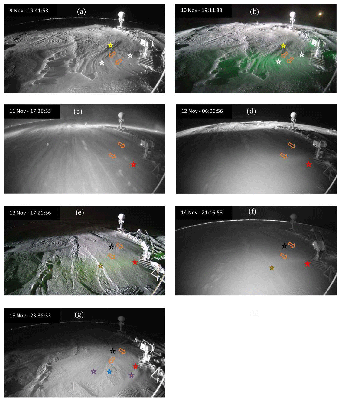
Figure 5Images of the RSS scan area between (a) 9 November and (g) 15 November. Images were selected during times of the day when the ship's floodlight was illuminating the scanning area. The KuKa radar is on the far right in the images, while an L-band scatterometer is on the upper right. Colored stars represent major snow bedforms within the KuKa radar scan area, while orange arrows show the orientation of the bedforms in response to the prevailing wind direction. All times are UTC.
Snow surface heights from TLS
The TLS-derived snow surface height data from 1, 8, and 15 November are illustrated in Fig. 6 along with superimposed green, buff, and magenta lines, indicating the centers of the radar scan area. Data from 1 November are included for context (left panel), indicating that the surface topography was similar to 8 November (middle panel). The TLS data illustrate considerable surface height variability within the radar scan area between 8 and 15 November, with snow surface height increasing (middle and right panel), as also indicated by the raised snow drift (black star in Fig. 5e–g) at approximately 0 to 45∘ azimuth in the CCTV images.
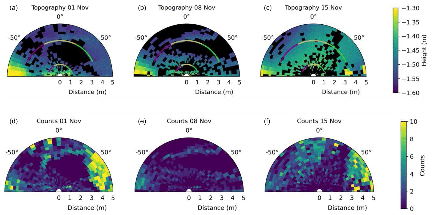
Figure 6TLS data (plan view) from 1, 8, and 15 November, from −90 to +90∘, where the angle indicates the azimuth of the radar positioner and radial horizontal distance measured from the center of the radar pedestal. Panels (a–c) show the topography as measured downwards (increasing negative) from the middle of the radar antenna arms. Black indicates no data recordings in that bin. Projections of the centers of the radar scan area are illustrated for 0 and 50∘ radar incidence angles between the −65 and +65∘ azimuth range, superimposed on the TLS data in magenta and green for radar observations, respectively, and buff where the two overlap, as per Fig. 1. Panels (d–f) indicate the number of TLS data points within each bin. Surface depressions resulting in 0 counts in the TLS data are due to obscuration by adjacent high areas due to snow–sea ice topography and human-made objects, as viewed from the TLS's oblique viewpoint some distance away.
3.2 Radar waveforms
Figure 7 shows the temporal progression of Ka- and Ku-band radar waveforms at nadir, overlaid with spatially coincident TLS-derived surface heights and averaged into individual 5∘ azimuth sectors. In the Video supplement, we provide an animation (Video S2) that includes all radar data from the two wind events, whereas here we show four timeframes to illustrate the radar response. As TLS data were acquired weekly, there are only these data available to overlay; in addition, as relatively few data points were available for 8 November, we also show data from 1 November – before the wind events. TLS data from all three dates are overlaid on all KuKa radar plots to demonstrate the time evolution of air–snow interface elevations in the two datasets.
Prior to WE1, radar waveforms remained stable, with only small power variations over time. The peak power at VV and HH generally corresponds to the air–snow interface in most θaz bins, as also confirmed by the TLS-derived heights. A lower scattering interface is visible at ∼ 20 to 40 cm below the air–snow interface, especially prominent in the HV data in both frequencies, and also in the VV and HH data. The range values indicated in the radar waveforms are based on the speed of light in free space. Correcting for a reduction of 80 % for snow (Willatt et al., 2009), the lower interfaces lay ∼ 16 to 32 cm below the air–snow interface. To better understand this, we consider the HV waveform and local snow depth. Snow depth measured behind the scan area during 4 and 14 November varied between 21 and 29 cm. Based on the very small amount of radiation scattered from larger ranges, negligible penetration of Ku- and Ka-band signals into sea ice, and the consistency with local snow depth, this interface in the HV data is very likely the snow–ice interface. A small amount of returned power is expected from beyond due to snow and ice backscattering from the perimeter of the 30–50 cm radar scan area and sidelobes.
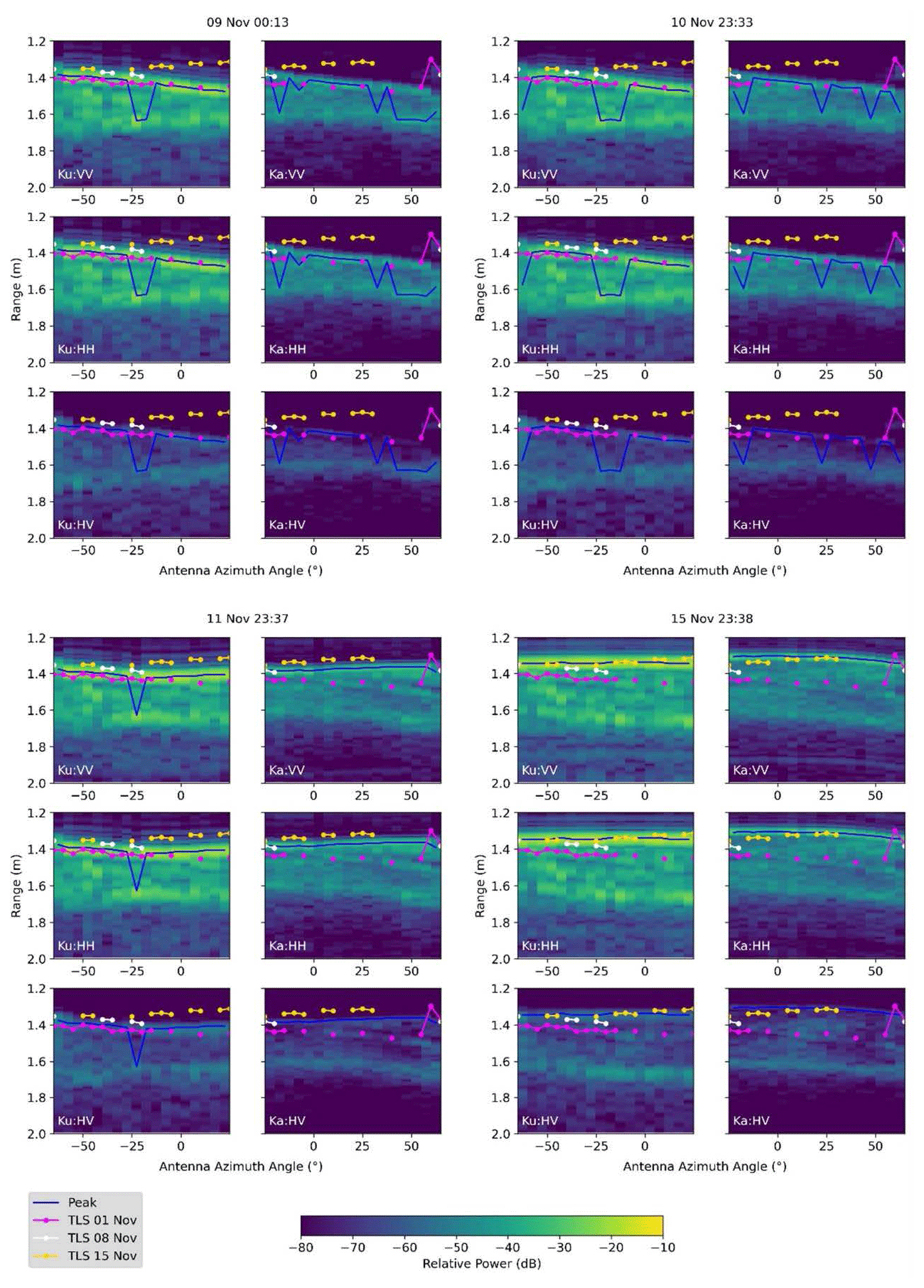
Figure 7Progression of Ka- and Ku-band radar power–depth profiles at nadir between −65 to +25∘ (Ku-band) and −25 to +65∘ (Ka-band) (azimuth ranges following Fig. 1e and f). Range (y axis) is given from the antenna phase center, and the antenna azimuth angles (x axis) are the angles for that individual antenna. The highest power peak (averaged across all polarizations) is indicated with a blue line, and the surface height in the spatially coincident TLS data is superimposed on top (colored circles).
During WE1, radar waveforms at nadir show that the peak power at the air–snow interface shifted upwards due to snow deposition at ∼ 18:00 UTC on 11 November (Fig. 5c). This is followed by a snow scouring/erosion event, seen in the downward movement of the peak power (Video S2), followed by a second deposition event at approximately 08:00 UTC on 12 November (Fig. 5d) and upward movement of the peak power (Fig. 8). It is interesting to note that the Ka- and Ku-band scattering can still be seen from the previous air–snow interface on 9 and 10 November (yellow arrows in Fig. 8), as well as from the snow–ice interface, more prominent in the Ku-band. After WE1, the new air–snow interface remains the dominant scattering surface for all polarizations and θaz sectors.
During WE2, after accumulation of newly redistributed snow, the air–snow interface moved upwards to a closer range from the antenna phase center (bottom right panel in Figs. 7 and 8). Scattering from the previously detected air–snow interface (corresponding to the TLS data from 1 and 8 November) is still visible in both Ka- and Ku-band data (Fig. 8). In addition, the air–snow interface from 11 November remains visible in the Ka-band data in all polarizations (bottom left panel in Fig. 7).
Next, we examined the highest amplitude peak at nadir and how this varies with frequency and polarization through time. Prior to WE1, the highest power peak originated from both air–snow and snow–ice interfaces at both frequencies (top panels in Fig. 7), suggesting variability in snow density (Fig. 4) and surface topography (Fig. 5) across the scan area. During and after WE1 and WE2, the highest peak power remains almost always at the air–snow interface for both frequencies (bottom panels in Fig. 7). This means that the backscatter values in the following Figs. 8 to 10 correspond to the air–snow or snow–ice interfaces, depending on the θaz sector and θinc, rather than to a change in backscatter from one interface. The TLS and radar waveforms also indicate a ∼ 2–5∘ slope in the radar scan area, especially at nadir (see Figs. 6 and 7). Sloped surfaces of 2–5∘ will significantly affect the total backscatter amplitude. However, since surface scattering is the dominant scattering mechanism at nadir, slightly sloped surfaces observed from the radar scan area likely do not affect the relative distribution of scattering between the air–snow and the snow–ice interfaces.
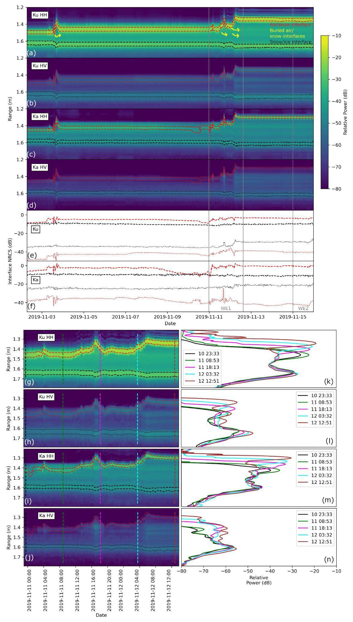
Figure 8Progression of the power–depth distributions over the commonly sampled area of the scan area between −25 and +25∘ θaz. The top panels (a)–(d) indicate the full time series from 2–15 November with the current air–snow and snow–ice interfaces indicated in red and black, respectively. Sketched yellow arrows show how buried air–snow interfaces remain visible through time. Individual air–snow and snow–sea ice interface NRCS values are determined by integrating the power between the red/black dashed/dotted lines, which cover the range bins where the power is within 2 dB from the air–snow and snow–sea ice interface peak. Time series of the interface NRCS values are illustrated below the echograms (panels (e) and (f)). The timings of WE1 and WE2 are indicated with grey lines and labels across panels (a) to (f). The bottom panels (g) to (j) show a temporal “zoom in” of WE1. Panels (k) to (n) show line plots of the waveforms at the given times corresponding to the vertical dashed lines on the echograms in (g) to (j).
Figure 8 illustrates the effect of WE1 and WE2 on HH-polarized waveform shapes and shows that the air–snow interface is always the dominant scattering surface in both frequencies. In the HV data, the snow–ice interface is the dominant scattering surface, but both interfaces are visible in both frequencies and all polarizations. Previous air–snow interfaces are also visible as in Fig. 7. The yellow arrows on the Ku-band HH plot show how the previous air–snow interfaces remain visible when additional snow accumulates. These buried interfaces, along with the snow–ice interface, appear at a greater range when covered with thicker snow due to the reduced wave propagation speed in snow relative to air, increasing the two-way travel time back to the radar receiver.
For the Ka- and Ku-band HH data, there are relatively small changes to the NRCS associated with the snow–ice interface (Fig. 8e and f), and changes associated with the air–snow interface are much larger. Prior to WE1, the Ka-band air–snow interface NRCS reduces from −5 to −10 dB before increasing during and after WE1 to −3 dB. At the Ku-band, a similar pattern is observed with the air–snow NRCS, reducing from −5 to −8 dB, then increasing to −3 dB following WE1. Most changes to NRCS from wind events relate to backscatter changes from the air–snow interface. The Ka-band HV data show the air–snow interface NRCS decreasing prior to WE1, increasing during the wind events, and then reducing to a lower value than previously, while the Ku-band data show the air–snow interface NRCS increasing during the wind events and remaining higher than previously. The different behavior at the two frequencies indicates that this could relate to roughness; i.e., the change in roughness is dependent on length scales. This is illustrated by further detail in the waveform line plots, which indicate how the waveform shape changed with more variability relating to the air–snow interface and snow above the snow–ice interface in both frequencies and polarizations. Both the Ka- and Ku-band HV show the snow–ice interface becoming brighter during the wind events and remaining brighter afterwards; we speculate that this may be related to temperature-gradient-driven metamorphism of basal snow.
3.3 Radar backscatter
This section focuses on the backscatter response from the overlapping area using azimuthally averaged Ka- and Ku-band backscatter time series at discrete θinc=0, 15, 35, and 50∘. Included are radar echograms at θinc=15 and 35∘ during WE1 to support backscatter interpretation. Two-dimensional interpolations of the spatial radar response along θinc and across 5∘ θaz bins over both Ka- and Ku-band scan areas separately are also used to analyze backscatter changes at specific times on 9, 11, and 15 November.
3.3.1 Azimuthally averaged backscatter
During pre-wind conditions, both Ka- and Ku-band backscatter are relatively stable (Fig. 9a, b). At nadir, VV and HH returns primarily originate from the air–snow interface. With higher values of θinc, air–snow interface scattering decreases due to the specular component of the backscattering not returning to the radar detector. The signal is therefore increasingly dominated by snow volume scattering and incoherent surface scattering at the snow–sea ice interface. HV backscatter originates primarily from the snow–sea ice interface (top panels in Fig. 7).
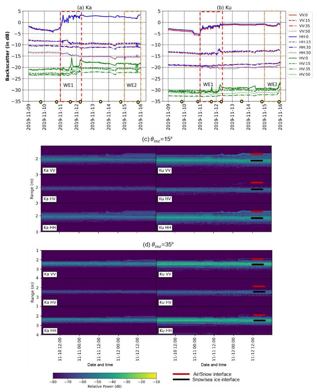
Figure 9Azimuthally averaged (a) Ka- and (b) Ku-band backscatter at 0, 15, 35, and 50∘ incidence angles between 9 and 16 November, from the overlapping −25 to +25∘ θaz area. Red and orange dotted sections indicate the WE1 and WE2 time window. Yellow circles correspond to times of the day (in UTC) when the CCTV camera captured snapshots of radar scans. Panels (c) and (d) show time series of Ka- and Ku-band radar echograms at (c) θinc=15∘ and (d) θinc=35∘ during WE1.
During WE1, nadir backscatter increases significantly, with a greater Ka-band increase of ∼ 8 dB (VV and HH), compared to a Ku-band increase of ∼ 5 dB (VV and HH) (Fig. 9a, b). The waveform analysis in Figs. 7 and 8 indicates that the amount of scattering from the snow–sea ice interface changed very little during WE1, while the scattering contribution to the backscatter from the air–snow interface increased significantly due to increasing snow density (Fig. 4) and decreasing radar-scale roughness (Fig. 5). This increase is accompanied by additional VV and HH backscatter from the previous, now-buried air–snow interface (Fig. 8). HV peak power shifts from the snow–sea ice interface to the air–snow interface and the buried within-snow interface (Fig. 8). This is clearly seen in the two significant HV increases at nadir, by up to 5 dB (Ka-band) and by up to 4 dB (Ku-band) during WE1 (Fig. 9a, b), coinciding with two short-term snow depositional events at ∼ 18:00 UTC on 11 November and around 07:00 UTC on 12 November (Fig. 5c, d and Video S1).
At θinc=15 and 35∘, the peak power interfaces during WE1 are much less obvious than at nadir but do exist (Fig. 9c, d). However, the bulk of the peak power moves from the air–snow interface to the snow–sea ice interface at all polarizations. The shifting of peak power from the air–snow interface to the snow–sea ice interface coincides with a decrease in Ka-band VV and HH backscatter by up to 2 dB at θinc=15∘ due to reduced air–snow interface roughness. The effect is less at θinc=35∘ due to the snow volume scattering becoming more dominant compared to surface/interface scattering at the slanting cross section at more oblique angles. The waveform analysis shows that the relative contribution of the snow–sea ice interface, snow volume scattering, and increased radar propagation delay due to increased snow accumulation become more important at shallow angles (Leinss et al., 2014), and the air–snow interface becomes relatively less prominent due to lower surface roughness after WE1. This feature is more observable in the HV data where the air–snow interface scattering is subtle, and the snow–sea ice interface is brighter, with potential snow and ice volume scattering (middle panels in Fig. 9c, d). The Ku-band at non-nadir incidence angles shows negligible change in HV backscatter (more stable in HV at θinc=35 and 50∘) compared to the Ka-band and pre-wind conditions (Fig. 9b). It is expected that the HV backscatter is dominated by volume scattering processes and that volume scattering is more prominent in the Ka-band because of the shorter wavelength.
During WE2, Ka- and Ku-band backscatter at all θinc remains relatively stable (Fig. 9a, b). Around ∼ 21:00 UTC on 15 November, a short-term snow depositional event (Video S1) causes the Ka-band nadir backscatter to increase by ∼ 2 dB. The Ka-band waveform analysis shows scattering contributions from the air–snow interface during the snow deposition and also from the previously detected air–snow interface from 11 November (Fig. 8 and lower-right panels in Fig. 7), causing the additional 2 dB increase. Similarly to WE1, Ku-band backscatter at θinc=35 and 50∘ remains nearly the same throughout WE2 (Fig. 9b). During WE2 it is likely that there is a slight snow surface roughness increase with a small nadir backscatter decrease and a small off-nadir increase.
3.3.2 Change in backscatter response at Δθaz=5∘
Changes in the spatial variation of the backscatter within each 5∘ θaz sector acquired at specific dates/times during pre-wind conditions to WE1 and WE2 are shown in Fig. 10. Compared to azimuthally averaged Ka- and Ku-band backscatter (Fig. 9), spatial variability in Ka- and Ku-band backscatter in response to wind events is evident at all polarizations and θinc. From pre-wind conditions to WE1, the most striking feature is the development of a drifted snow dune directly in front of the sled (red star in Fig. 5) at θinc < 10∘, which led to an increase in Ka- and Ku-band backscatter by up to 9 dB, at nadir throughout all θaz sectors. Beyond θinc=10∘, the changes in Ka-band VV and HH backscatter are primarily negative, with spatially heterogeneous areas of positive change primarily in the θaz sectors >20∘ at θinc>30∘. The change in Ka-band HV backscatter at θinc<10∘ is more consistently positive at θaz sectors < 0∘, and it agrees well with the strong HV backscatter increase related to deeper snow during the first snow depositional event that occurred halfway through WE1 on 11 November (Fig. 5 and Video S1).
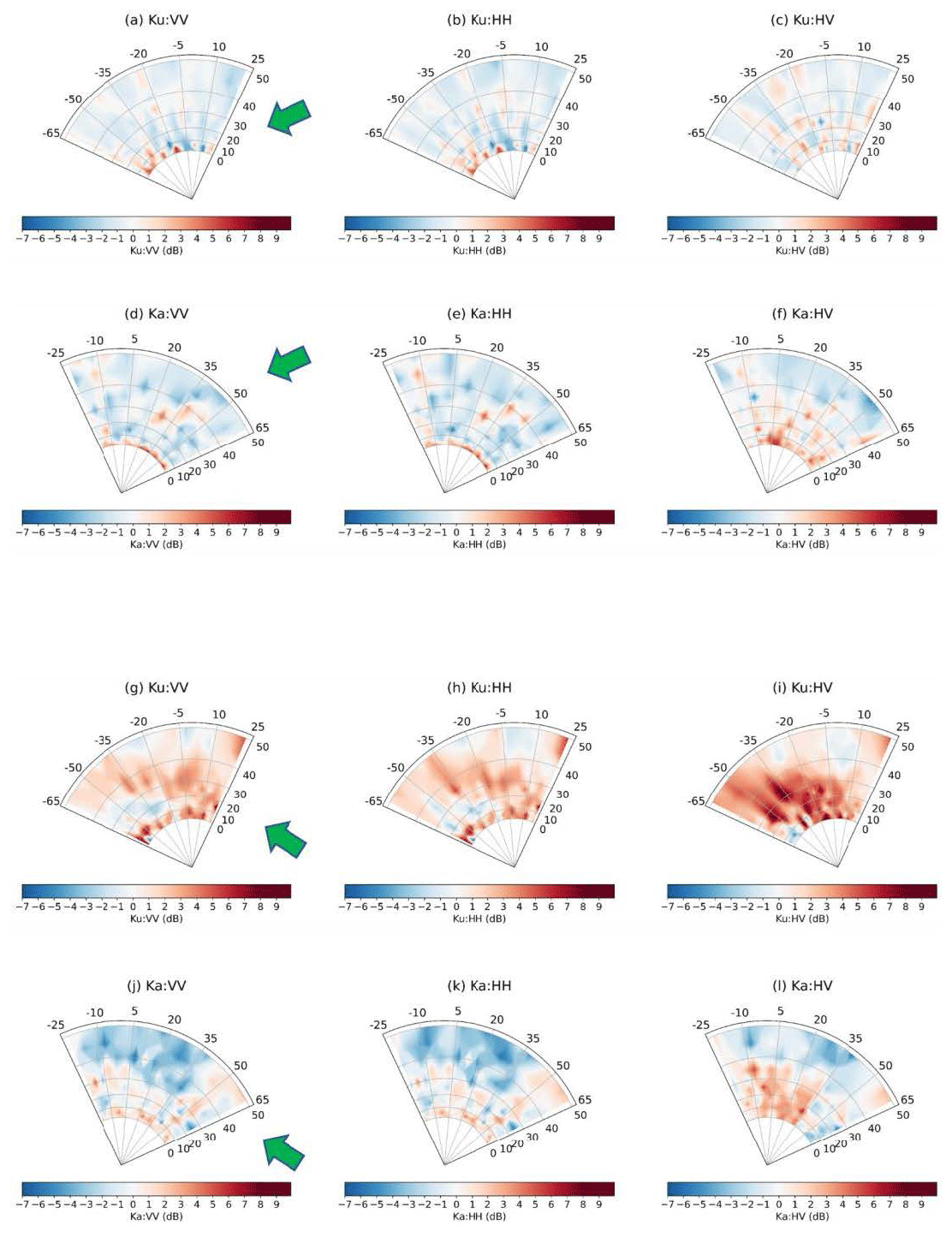
Figure 10Polar plot panels (a) to (f) show the relative change in averaged Ku- and Ka-band backscatter at 5∘ azimuth sectors, as a function of θinc, between WE1 and pre-wind conditions, acquired on 11 (WE1) and 9 November at 23:37 and 00:13 UTC, respectively. Panels (g) to (l) show the same between windy conditions, acquired on 11 (WE1) and 15 (WE2) November, at 23:37 and 23:38 UTC, respectively. Green arrows in (a) and (g) denote the prevailing wind direction on 11 and 15 November, respectively. The scan times also correspond to yellow circles in Fig. 9 and CCTV images in Fig. 5a and c. Note: the 11 November CCTV image in Fig. 5c is acquired at 17:36 UTC for image clarity showing blowing snow.
WE2 produces a stronger response in Ka- and Ku-band backscatter across the θaz sectors compared to WE1. Ka-band VV and HH backscatter change is primarily negative (up to 7 dB) at θinc>30∘, while Ka- and Ku-band HV backscatter shows strong positive change (up to 9.5 dB) at θinc>40∘. Images in Fig. 5 and TLS scans from 8 and 15 November illustrate changes in surface heights due to the drifts that formed towards the left side of the KuKa radar (purple stars in Fig. 5), and the deeper snow appears to be captured by a strongly enhanced Ku-band HV response at θaz sectors < 0∘. The large backscatter changes along these sectors align with the wind direction and also indicate change in snow topography caused by snow blown from behind the radar.
4.1 Impact of snow redistribution on radar signatures
Our analyses demonstrate that Ka- and Ku-band backscatter and waveforms are sensitive to wind-induced snow redistribution. During pre-wind conditions, the dominant radar scattering surface at nadir for both frequencies at the co-polarized channels switches between the air–snow and snow–sea ice interfaces depending on local variations in snow surface density and roughness. HV backscatter surface changes as a function of snow depth. This is illustrated by the waveform analysis, with the range to the air–snow interface confirmed by georeferencing the radar and TLS data (Figs. 7 and 8 and Video S2) and the range to the snow–sea ice interface inferred from local snow depth measurements and the strong interface contrast evident in backscatter in the radar waveforms and the opposite changes (increase/decrease) in the nadir and off-nadir backscatter. Following WE1, the air–snow interface becomes the dominant scattering surface at nadir at all polarizations due to the smoothening of the snow surface combined with the increased snow surface density. At satellite scales, this may upwardly shift the retracked elevation and resulting sea ice freeboard retrievals by radar altimeters that assume the snow–sea ice interface is the dominant scattering surface. This would introduce an overestimating bias on the sea ice thickness estimate; however, a number of other uncertainties are also at play in this process, meaning this may move the retrieval closer to or further from the true value. Our surface-based findings are consistent with recent satellite-based work by Nab et al. (2023), who showed a temporary lifting of CryoSat-2-derived radar freeboard in response to snow accumulation but also higher wind speeds and warmer air temperatures. Due to snow surface smoothening at non-nadir incidence angles, the relative scattering contribution of the snow–sea ice interface compared to the air–snow interface increases, and the air–snow interface gradually becomes invisible (Fig. 9).
The Ku- and Ka-band radar backscatter is still sensitive to the presence of buried and historical air–snow interfaces within the snowpack (Figs. 7–9), which indicates that snow density and/or surface roughness contrasts (Fig. 4) existing prior to wind events continue to influence scattering even once additional snow is deposited (Fig. 8). This is an important finding because even if an interface is not the dominant scattering surface, it can affect the waveform shape and assumptions about the surface elevation retrieved from airborne and satellite radar altimetry data when there is no a priori information on the snow geophysical history. In future studies, gathering TLS data on the snow surface roughness at high spatial (radar) and temporal (e.g., daily or hourly) resolution would provide valuable information on the role of roughness. In addition, collecting near-coincident measurements of snow density would provide information on the role of density affecting radar waveforms. We would therefore recommend collecting these coincident datasets in future similar studies.
The relatively small backscatter observed from the snowpack at θinc=15 and 35∘ (Fig. 9c, d) indicates dominant scattering away from the radar. At these angles, most of the backscatter is associated with the snow–sea ice interface, and deeper snow is causing an increasing slant-range delay. The air–snow interface is directly impacted by the wind, experiencing compaction to higher snow density and reduced surface roughness (Figs. 4 and 5). The NRCS associated with the air–snow interface increased by more than 5 dB during and following the wind events (Fig. 8). Thus, utilizing time series backscatter at both near- and off-nadir incidence angles may be useful for retrieving snow surface roughness and/or density changes, though it may be difficult to separate these variables.
This study does not replicate airborne- and satellite-scale conditions (e.g., beam geometry, snow cover, and ice-type variability on satellite scales). Therefore, the waveform shape, return peak power, and measured backscatter from the KuKa radar will be different from airborne and satellite radar altimeters and scatterometers. Also of note is the highly localized nature of the radar backscatter, which is a function of small-scale surface roughness combined with local θinc that includes some steep angles due to snow drifts and bedforms in the scan area. Even at nadir-viewing geometry, the beam-limited KuKa radar scan area covers an angular range of 12–17∘, which is many orders of magnitude larger than the beamwidth of a satellite altimeter's antenna and 2 orders of magnitude larger than the equivalent beamwidth of the altimeter's pulse-limited footprint, which for CryoSat-2 is around 0.1∘ (Wingham et al., 2006).
The relative dominance of coherent over non-coherent backscatter mechanisms can vary significantly within the KuKa beamwidth alone, with coherent reflections from near-specular surfaces dominating the radar response more easily at satellite scales (Fetterer et al., 1992). However, even from a satellite-viewing geometry, a smooth air–snow interface should produce sufficient backscattering at the Ku-band to modify the leading edge of the altimeter waveform response (Landy et al., 2019). The larger satellite footprints may also include different surfaces, such as pressure ridges, rafting and rubble fields, hummocks, refrozen leads, level first-year sea ice, and open water. The effects of small-scale roughness, larger-scale topography, and sub-beamwidth θinc would combine in different ways for larger footprints, such as from satellites operating at large θinc, where the distribution of local θinc may be less extreme, and the signal would be dominated by the smooth parts of the surface (e.g., Segal et al., 2020).
As mentioned earlier, the KuKa radar has a much higher vertical resolution than CryoSat-2 and AltiKa. This means that although the individual interfaces would not be resolved in the satellite data, the waveform shape and hence retrieved elevation could be affected by current, recent (days), and historical (weeks or longer) timescales of wind-driven redistribution changes to the snow topography and physical properties. Retracking algorithms do not yet factor in the potential leftwards migration (shortening range) of the waveform leading edge that could be caused by radar responses from the snow surface and historically buried snow interfaces.
4.2 The azimuth sectoring approach and interdependence of wind and snow properties on backscatter
Azimuth sectoring provides an assessment of the backscatter heterogeneity across the radar scan area, here linked to the dynamic evolution of snow bedforms during wind events. Our results show how sensitive the KuKa backscatter is to development of snow bedforms and changing snow surface heights within the scan area with a directionality corresponding to prevailing wind speed and direction.
The demonstrated influence of snowscape evolution from wind events prompts the need for further investigation of the relative contributions of snow density, surface roughness, and snow grain size to Ka- and Ku-band backscatter. There are three main considerations: (1) measurement and parameterization of snow surface roughness on the scale of the radar wavelength are poorly understood, especially with regard to temporal variability; (2) wind induces rapid density evolution at the snow surface (Filhol and Sturm, 2015); and (3) strong covariance exists between snow density, snow temperature gradient metamorphosis, and snow grain size (Colbeck, 1989). Although there is no time series of density profiles available for the RSS, we show a clear increase in the density of the upper snowpack within profiles at comparable locations nearby the RSS (Fig. 4). As a snow surface densifies, surface scattering increases due to the enhanced dielectric contrast. Moreover, as snow warms, temperature-gradient-driven metamorphism leads to density changes, which can also modify the roughness of the surface and/or internal interfaces, resulting in changes to backscatter (Lacroix et al., 2009).
The waveform analysis provides some insights into the effects of wind vs. temperature. In a previous study, the significant increase in C-band backscatter after a storm was attributed to enhanced radar-scale snow surface roughness and increasing moisture content in snow with temperatures 6 ∘C (Komarov et al., 2017). Strong contributions from snow grain volume scattering at C-band prior to the storm were masked by dominant surface scattering after wind roughening and mechanical breakup of the snow grains during wind redistribution. In our study, the air and snow surface temperature did not reach −12 ∘C until late on 11 November (Figs. 2 and 3), but the increasing wind speeds during WE1 (Fig. 2) were already switching the dominant scattering surface from being a mixture of the air–snow and snow–ice interface (prior to the wind events) to almost exclusively being the air–snow interface and increasing the backscatter associated with the air–snow interface by ∼ 5 dB (Fig. 8). The action of the wind on the snow surface dominated the change in the scattering surface. Therefore, we suggest the effect of the wind on the snow roughness and/or on the snow density (wind compaction of the top layer) (Fig. 4) causes the air–snow interface to increasingly become the dominant scattering surface at Ka- and Ku-band frequencies.
This study details the impact of two wind events on surface-based Ka- and Ku-band radar signatures of snow on Arctic sea ice, collected during the MOSAiC expedition in November 2019. The formation of snow bedforms and erosion events in the radar scan area modified the snow surface heights, and this was recorded consistently by the radar instrument, a terrestrial laser scanner, and optical imagery. Analysis of radar waveforms demonstrated that the air–snow and snow–sea ice interfaces are visible in both frequencies and all polarizations and incidence angles. During wind events, buried air–snow interfaces remain clearly detectable at nadir, following new snow deposition. This shows that the historical conditions under which a snow cover evolves, rather than only current conditions, affect backscatter.
We conclude that wind action and its effect on snow density and surface roughness, rather than temperature, which remained < −10 ∘C during the first recorded backscatter shifts, caused the observed change in the dominant scattering interface from a mixture of air–snow and snow–sea ice interfaces to predominantly the air–snow interface, and nadir backscatter at the air–snow interface increased by up to 5 dB. This effect would likely also be manifested in waveforms detected by satellite altimeters operating at the same frequencies, e.g., AltiKa or CryoSat-2.
Compared to pre-wind conditions, nadir backscatter across the full radar azimuth increased by up to 8 dB (Ka-band) and by up to 5 dB (Ku-band) during the wind events. This was caused by the formation of snow bedforms within the radar scan area, which increased the snow surface roughness and/or density. Spatial variability in backscatter was evident across the radar scan area and that variability responded to the formation and evolution of snow bedforms, which in turn was driven by increasing wind speeds and changing wind direction.
Overall, our results from the KuKa radar provide a process-scale understanding of how wind redistribution of snow on sea ice can affect its topography and physical properties and how these changes in turn can affect the radar properties of the snow cover. Our results are relevant to both satellite altimetry and scatterometry through changes to radar waveforms and backscatter during and after wind events. However, more investigation is needed to deduce how much wind (i.e., conditions/thresholds across space and time) is needed to impact satellite waveforms. Our findings cannot be applied directly to satellite instruments without considering differences in footprint sizes, incidence angles, and the snow and sea ice properties sampled. However, we do provide first-hand information on the frequency, incidence angle, and polarization responses of snow on sea ice, which are important for modeling scattered radiation over an airborne and satellite footprint.
In future field-based experiments, we will aim to combine near-coincident KuKa radar data and snow depth measurements (Stroeve et al., 2020), terrestrial laser scanner measurements of snow surface roughness, and snow density profiles to better characterize the effect of these variables on the radar range measurements. Forthcoming KuKa radar deployments on Antarctic sea ice will produce further insights into snow geophysical processes (e.g., presence of slush, melt–refreeze layers, snow ice formation etc.) that may affect snow depth and sea ice thickness retrievals from satellite radar altimetry. In a windy Arctic and the Antarctic, these methods will facilitate improved insights towards better quantifying the impact of snow redistribution on accurate retrievals of snow–sea ice parameters from satellite radar missions such as SARAL/AltiKa, CryoSat2, Sentinel-3A, Sentinel-6, SWOT, CRISTAL, and ScatSat-1.
KuKa radar data were processed using the KuKaPy Python framework available in https://doi.org/10.5281/zenodo.7967058 (vishnu-seaice, 2023). Data used in this paper were produced as part of the international Multidisciplinary drifting Observatory for the Study of the Arctic Climate (MOSAiC) expedition with the tag MOSAiC20192020 and project ID AWI PS122 00. Optical camera data from the remote sensing site are available at https://doi.org/10.1594/PANGAEA.939362 (Spreen et al., 2021). Infrared camera data from the remote sensing site are available at https://doi.org/10.1594/PANGAEA.940717 (Spreen et al., 2022). KuKa radar data are available at https://doi.org/10.5285/0caf5c54-9a40-4a96-a39b-b5c9c2863271 (Stroeve et al., 2022).
The time-lapse video of wind events acquired by the CCTV camera (supplemental Video S1, https://doi.org/10.5446/56641; Spreen and Huntemann, 2022) and an animation of radar and TLS waveforms during the wind events (supplemental Video S2, https://doi.org/10.5446/57132; Willatt and Clemens-Sewall, 2022) are provided.
VN processed the KuKa radar data and wrote the paper with input from co-authors. RW processed and analyzed the KuKa radar waveforms including NRCS calculations of interfaces, overlaid TLS data on radar waveforms, and produced the radar and TLS time series animation. RM processed and plotted the DTC data. DCS processed the TLS data from the raw format and wrote code for plotting and analysis of TLS data used in this paper. AJ produced the floe map for the paper. DW and DK processed the SMP data, and DW produced the SMP plot. JS, RS, TG, and JL provided extensive inputs and reviews on the paper. RT, JY, TN, DJ, MH, JM, GS, SH, RR, MT, MM, MS, DW, MG, CD, IR, CP, IM, and MH provided valuable editorial comments. Many co-authors helped collect data during MOSAiC.
The contact author has declared that none of the authors has any competing interests.
Publisher’s note: Copernicus Publications remains neutral with regard to jurisdictional claims in published maps and institutional affiliations.
This work was carried out as part of the international Multidisciplinary drifting Observatory for the Study of the Arctic Climate (MOSAiC) expedition, MOSAiC20192020. We thank all scientific personnel and crew members involved in the expedition of the research vessel Polarstern during MOSAiC in 2019–2020 (AWI_PS122_00) and Thomas Johnson (University College London) for advising on plots and animations.
This research has been supported by the European Space Agency (grant no. 5001027396), the European Organization for the Exploitation of Meteorological Satellites (grant no. 4500019119), the Swiss Polar Institute (grant no. EXF-2018-003), the Horizon 2020 (ARICE grant (no. 730965)), the Deutsche Forschungsgemeinschaft (grant no. 221211316), the Bundesministerium für Bildung, Wissenschaft, Forschung und Technologie (grant no. 03F0866B), the Natural Environment Research Council (grant nos. NE/S002510/1 and NE/L002485/1), the Canada Research Chairs (grant no. G00321321), and the Natural Sciences and Engineering Research Council of Canada (grant no. PDF-557649-2021). Meteorological data collection was funded by the National Science Foundation (grant no. OPP-1724551).
This project has received funding from the European Union's Horizon 2020 research and innovation program (grant no. 01003826). VN was additionally supported by Canada's Marine Environmental Observation, Prediction and Response Network (MEOPAR) postdoctoral funds. MG was supported by the DOE Atmospheric System Research program (grant nos. DE-SC0019251, DE-SC0021341). GS, MH, AJ, and SH were supported by the German Ministry for Education and Research (BMBF) through the MOSAiC IceSense projects (grant no. 03F0866B to GS and MH and grant no. 03F0866A to AJ and SH) and by the Deutsche Forschungsgemeinschaft (DFG) through the International Research Training Group IRTG 1904 ArcTrain (grant no. 221211316). MS and DW were supported by the European Union's Horizon 2020 research program (ARICE grant no. 730965) for MOSAiC berth fees associated with the DEARice participation and the Swiss Polar Institute grant SnowMOSAiC (grant no. EXF-2018-003). CD was funded through the EUMETSAT MOSAiC project (grant no. 4500019119).
This paper was edited by Melody Sandells and reviewed by Nathan Kurtz and Silvan Leinss.
Armitage, T. W. and Kwok, R.: SWOT and the ice-covered polar oceans: An exploratory analysis, Adv. Space Res., 68, 829–842, https://doi.org/10.1016/j.asr.2019.07.006, 2021.
Armitage, T. W. and Ridout, A. L.: Arctic sea ice freeboard from AltiKa and comparison with CryoSat-2 and Operation IceBridge, Geophy. Res. Lett., 42, 6724–6731, https://doi.org/10.1002/2015GL064823, 2015.
Clemens-Sewall, D., Parno, M., Perovich, D., Polashenski, C., and Raphael, I. A.: FlakeOut: A geometric approach to remove wind-blown snow from terrestrial laser scans, Cold Reg. Sci. Tech., 201, 103611, https://doi.org/10.1016/j.coldregions.2022.103611, 2022.
Colbeck, S. C.: Snow-crystal growth with varying surface temperatures and radiation penetration, J. Glaciol., 35, 23–29, https://doi.org/10.3189/002214389793701536, 1989.
Cox, C., Gallagher, M., Shupe, M., Persson, O., and Solomon, A.: 10-meter (m) meteorological flux tower measurements (Level 1 Raw), Multidisciplinary Drifting Observatory for the Study of Arctic Climate (MOSAiC), central Arctic, October 2019–September 2020, Arctic Data Center, https://doi.org/10.18739/A2VM42Z5F, 2021.
Doviak, R. J. and Zrnić, D.: Doppler Radar and Weather Observations, Academic Press, 458 pp., https://doi.org/10.1016/B978-0-12-221422-6.50007-3, 1993.
Fetterer, F. M., Drinkwater, M. R., Jezek, K. C., Laxon, S. W., Onstott, R. G., and Ulander, L. M.: Sea ice altimetry, Washington DC, Amer. Geophy. Uni. Geophy, Mono. Ser., 68, 111–135, 1992.
Filhol, S. and Sturm, M.: Snow bedforms: A review, new data, and a formation model, Journal Geophy. Res.-Earth Surf., 120, 1645–1669, https://doi.org/10.1002/2015JF003529, 2015.
Guerreiro, K., Fleury, S., Zakharova, E., Rémy, F., and Kouraev, A.: Potential for estimation of snow depth on Arctic sea ice from CryoSat-2 and SARAL/AltiKa missions, Remote Sens. Environ., 186, 339–349, https://doi.org/10.1016/j.rse.2016.07.013, 2016.
Iacozza, J. and Barber, D. G.: An examination of snow redistribution over smooth land-fast sea ice, Hydrol. Process., 24, 850–865, https://doi.org/10.1002/hyp.7526, 2010.
Johnson, J. B. and Schneebeli, M.: Characterizing the microstructural and micromechanical properties of snow, Cold Reg. Sci. Tech., 30, 91–100, https://doi.org/10.1016/S0165-232X(99)00013-0, 1999.
Kern, M., Cullen, R., Berruti, B., Bouffard, J., Casal, T., Drinkwater, M. R., Gabriele, A., Lecuyot, A., Ludwig, M., Midthassel, R., Navas Traver, I., Parrinello, T., Ressler, G., Andersson, E., Martin-Puig, C., Andersen, O., Bartsch, A., Farrell, S., Fleury, S., Gascoin, S., Guillot, A., Humbert, A., Rinne, E., Shepherd, A., van den Broeke, M. R., and Yackel, J.: The Copernicus Polar Ice and Snow Topography Altimeter (CRISTAL) high-priority candidate mission, The Cryosphere, 14, 2235–2251, https://doi.org/10.5194/tc-14-2235-2020, 2020.
King, J., Howell, S., Brady, M., Toose, P., Derksen, C., Haas, C., and Beckers, J.: Local-scale variability of snow density on Arctic sea ice, The Cryosphere, 14, 4323–4339, https://doi.org/10.5194/tc-14-4323-2020, 2020.
Komarov, A. S., Landy, J. C., Komarov, S. A., and Barber, D. G.: Evaluating scattering contributions to C-band radar backscatter from snow-covered first-year sea ice at the winter–spring transition through measurement and modelling, IEEE Trans. Geosci. Remote Sens., 55, 5702–5718, https://doi.org/10.1109/TGRS.2017.2712519, 2017.
Kurtz, N. T. and Farrell, S. L.: Large-scale surveys of snow depth on Arctic sea ice from Operation IceBridge, Geophy. Res. Lett., 38, L20505, https://doi.org/10.1029/2011GL049216, 2011.
Lacroix, P., Legresy, B., Remy, F., Blarel, F., Picard, G., and Brucker, L.: Rapid change of snow surface properties at Vostok, East Antarctica, revealed by altimetry and radiometry, Remote Sens. Environ., 113, 2633–2641, https://doi.org/10.1016/j.rse.2009.07.019, 2009.
Landy, J. C., Tsamados, M., and Scharien, R. K.: A facet-based numerical model for simulating SAR altimeter echoes from heterogeneous sea ice surfaces, IEEE Trans. Geosci. Remote Sens., 57, 4164–4180, https://doi.org/10.1109/TGRS.2018.2889763, 2019.
Lawrence, I. R., Tsamados, M. C., Stroeve, J. C., Armitage, T. W. K., and Ridout, A. L.: Estimating snow depth over Arctic sea ice from calibrated dual-frequency radar freeboards, The Cryosphere, 12, 3551–3564, https://doi.org/10.5194/tc-12-3551-2018, 2018.
Lawrence, I. R., Armitage, T. W., Tsamados, M. C., Stroeve, J. C., Dinardo, S., Ridout, A. L., Tilling, R. L., and Shepherd, A.: Extending the Arctic sea ice freeboard and sea level record with the Sentinel-3 radar altimeters, Adv. Space Res., 68, 711–723, https://doi.org/10.1016/j.asr.2019.10.011, 2021.
Leinss, S., Lemmetyinen, J., Wiesmann, A., and Hajnsek, I.: Snow Structure Evolution Measured by Ground Based Polarimetric Phase Differences, in: EUSAR- 2014, 10th European Conference on Synthetic Aperture Radar (1–4 pp.), https://ieeexplore.ieee.org/servlet/opac?punumber=6856711 (last access: 17 May 2023), VDE, 2014.
Löwe, H., Egli, L., Bartlett, S., Guala, M., and Manes, C.: On the evolution of the snow surface during snowfall, Geophys. Res. Lett., 34, L21507, https://doi.org/10.1029/2007GL031637, 2007.
Moon, W., Nandan, V., Scharien, R. K., Wilkinson, J., Yackel, J. J., Barrett, A., Lawrence, I., Segal, R. A., Stroeve, J., Mahmud, M., Duke, P. J., and Else, B.: Physical length scales of wind-blown snow redistribution and accumulation on relatively smooth Arctic first-year sea ice, Environ. Res. Lett., 14, 104003, https://doi.org/10.1088/1748-9326/ab3b8d, 2019.
Nab, C., Mallett, R., Gregory, W., Landy, J., Lawrence, I., Willatt, R., Stroeve, J., and Tsamados, M.: Synoptic variability in satellite altimeter-derived radar freeboard of Arctic sea ice, Geophy. Res. Lett., 50, e2022GL100696, https://doi.org/10.1029/2022GL100696, 2023.
Nandan, V., Scharien, R., Geldsetzer, T., Mahmud, M., Yackel, J. J., Islam, T., Gill, J. P. S., Fuller, M. C., and Grant, G., and Duguay, C.: Geophysical and atmospheric controls on Ku-, X-and C-band backscatter evolution from a saline snow cover on first-year sea ice from late-winter to pre-early melt, Remote Sens. Environ., 198, 425–441, https://doi.org/10.1016/j.rse.2017.06.029, 2017.
Nicolaus, M., Perovich, D. K., Spreen, G., et al.: Overview of the MOSAiC expedition: Snow and sea ice, Elem. Sci. Anth., 10, 000046, https://doi.org/10.1525/elementa.2021.000046, 2022.
Proksch, M., Löwe, H., and Schneebeli, M.: Density, specific surface area, and correlation length of snow measured by high-resolution penetrometry, J. Geophy. Res.-Earth Surf., 120, 346–362, https://doi.org/10.1002/2014JF003266, 2015.
Savelyev, S. A., Gordon, M., Hanesiak, J., Papakyriakou, T., and Taylor, P. A.: Blowing snow studies in the Canadian Arctic shelf exchange study, 2003–04, Hydrol. Process., 20, 817–827, https://doi.org/10.1002/hyp.6118, 2006.
Segal, R. A., Scharien, R. K., Cafarella, S., and Tedstone, A.: Characterizing winter landfast sea-ice surface roughness in the Canadian Arctic Archipelago using Sentinel-1 synthetic aperture radar and the Multi-angle Imaging SpectroRadiometer, Ann. Glaciol., 61, 284–298, https://doi.org/10.1017/aog.2020.48, 2020.
Singh, U. S. and Singh, R. K.: Application of maximum-likelihood classification for segregation between Arctic multi-year ice and first-year ice using SCATSAT-1 data, Rem. Sens. Appl.-Society Environ., 100310, https://doi.org/10.1016/j.rsase.2020.100310, 2020.
Spreen, G. and Huntemann, M.: CCTV Footage of the remote sensing footprint between 9 and 16 November 2019 from the MOSAiC Expedition, Logo TIB AV-Portal [Video], https://doi.org/10.5446/56641, 2022.
Spreen, G., Huntemann, M., Naderpour, R., Mahmud, M., Tavri, A., and Thielke, L.: Optical IP Camera images (VIS_INFRALAN_01) at the remote sensing site on the ice floe during MOSAiC expedition 2019/2020, PANGAEA [data set], https://doi.org/10.1594/PANGAEA.939362, 2021.
Spreen, G., Huntemann, M., Thielke, L., Naderpour, R., Mahmud, M., and Tavri, A.: Infrared camera raw data (ir_variocam_01) at the remote sensing site on the ice floe during MOSAiC expedition 2019/2020, PANGAEA [data set], https://doi.org/10.1594/PANGAEA.940717, 2022.
Stroeve, J., Nandan, V., Willatt, R., Tonboe, R., Hendricks, S., Ricker, R., Mead, J., Mallett, R., Huntemann, M., Itkin, P., Schneebeli, M., Krampe, D., Spreen, G., Wilkinson, J., Matero, I., Hoppmann, M., and Tsamados, M.: Surface-based Ku- and Ka-band polarimetric radar for sea ice studies , The Cryosphere, 14, 4405–4426, https://doi.org/10.5194/tc-14-4405-2020, 2020.
Stroeve, J., Nandan, V., Tonboe, R., Hendricks, S., Ricker, R., and Spreen, G.: Ku- and Ka-band polarimetric radar backscatter of Arctic sea ice between October 2019 and September 2020 – VERSION 2.0, NERC BAS [data set], https://doi.org/10.5285/0caf5c54-9a40-4a96-a39b-b5c9c2863271, 2022.
Tilling, R. L., Ridout, A., and Shepherd, A.: Estimating Arctic sea ice thickness and volume using CryoSat-2 radar altimeter data, Adv. Space Res., 62, 1203–1225, https://doi.org/10.1016/j.asr.2017.10.051, 2018.
Trujillo, E., Leonard, K., Maksym, T., and Lehning, M.: Changes in snow distribution and surface topography following a snowstorm on Antarctic sea ice, J. Geophys. Res.-Earth Surf., 121, 2172– 2191, https://doi.org/10.1002/2016JF003893, 2016.
Ulaby, F. T., Long, D. G., Blackwell, W. J., Elachi, C., Fung, A. K., Ruf, C., Sarabandi, K., Van Zyl, J., and Zebker, H.: Microwave radar and radiometric remote sensing (Vol. 4, No. 5, p. 6). Ann Arbor, MI, USA: University of Michigan Press, ISBN 978-0-472-11935-6, 2014.
Virtanen, P., Gommers, R., Oliphant, T. E., Haberland, M., Reddy, T., Cournapeau, D., Burovski, E., Peterson, P., Weckesser, W., Bright, J., van der Walt, S. J., Brett, M., Wilson, J., Jarrod Millman, K., Mayorov, N., Nelson, A. R. J., Jones, E., Kern, R., Larson, E., Carey, C. J., Polat, İ., Feng, Y., Moore, E. W., VanderPlas, J., Laxalde, D., Perktold, J., Cimrman, R., Henriksen, I., Quintero, E. A., Harris, C. R., Archibald, A. M., Ribeiro, A. H., Pedregosa, F., van Mulbregt, P., and SciPy 1.0 Contributors: SciPy 1.0: fundamental algorithms for scientific computing in Python, Nat. methods, 17, 261–272, https://doi.org/10.1038/s41592-019-0686-2, 2020.
vishnu-seaice: vishnu-seaice/KuKaPy: Python code to process Ku- and Ka-band polarimetric radar data (Version v1), Zenodo [data set], https://doi.org/10.5281/zenodo.7967058, 2023.
Wagner, D. N., Shupe, M. D., Cox, C., Persson, O. G., Uttal, T., Frey, M. M., Kirchgaessner, A., Schneebeli, M., Jaggi, M., Macfarlane, A. R., Itkin, P., Arndt, S., Hendricks, S., Krampe, D., Nicolaus, M., Ricker, R., Regnery, J., Kolabutin, N., Shimanshuck, E., Oggier, M., Raphael, I., Stroeve, J., and Lehning, M.: Snowfall and snow accumulation during the MOSAiC winter and spring seasons, The Cryosphere, 16, 2373–2402, https://doi.org/10.5194/tc-16-2373-2022, 2022.
Wingham, D. J., Francis, C. R., Baker, S., Bouzinac, C., Brockley, D., Cullen, R., De Chateau-Thierry, P., Laxon, S. W., Mallow, U., Mavrocordatos, C., Phalippou, L., Ratier, G., Rey, L., Rostan, F., Viau, P., and Wallis, D. W.: CryoSat: A mission to determine the fluctuations in Earth's land and marine ice fields, Adv. Space Res., 37, 841–871, https://doi.org/10.1016/j.asr.2005.07.027, 2006.
Willatt, R. and Clemens-Sewall, D.: Ranging Analysis of KuKa Radar on snow-covered Arctic sea ice during MOSAiC Expedition, Logo TIB AV-Portal [Video], https://doi.org/10.5446/57132, 2022.
Willatt, R. C., Giles, K. A., Laxon, S. W., Stone-Drake, L., and Worby, A. P.: Field investigations of Ku-band radar penetration into snow cover on Antarctic sea ice, IEEE Trans. Geosci. Remote Sens., 48, 365–372, https://doi.org/10.1109/TGRS.2009.2028237, 2009.
Yackel, J. J. and Barber, D. G.: Observations of snow water equivalent change on landfast first-year sea ice in winter using synthetic aperture radar data, IEEE Trans. Geosci. Remote Sens., 45, 1005–1015, https://doi.org/10.1109/TGRS.2006.890418, 2007.