the Creative Commons Attribution 4.0 License.
the Creative Commons Attribution 4.0 License.
 | 25 May 2023
Forcing and impact of the Northern Hemisphere continental snow cover in 1979–2014
Guillaume Gastineau
Claude Frankignoul
Yongqi Gao
Yu-Chiao Liang
Young-Oh Kwon
Annalisa Cherchi
Rohit Ghosh
Elisa Manzini
Daniela Matei
Jennifer Mecking
Lingling Suo
Tian Tian
Shuting Yang
Ying Zhang
The main drivers of the continental Northern Hemisphere snow cover are investigated in the 1979–2014 period. Four observational datasets are used as are two large multi-model ensembles of atmosphere-only simulations with prescribed sea surface temperature (SST) and sea ice concentration (SIC). A first ensemble uses observed interannually varying SST and SIC conditions for 1979–2014, while a second ensemble is identical except for SIC with a repeated climatological cycle used. SST and external forcing typically explain 10 % to 25 % of the snow cover variance in model simulations, with a dominant forcing from the tropical and North Pacific SST during this period. In terms of the climate influence of the snow cover anomalies, both observations and models show no robust links between the November and April snow cover variability and the atmospheric circulation 1 month later. On the other hand, the first mode of Eurasian snow cover variability in January, with more extended snow over western Eurasia, is found to precede an atmospheric circulation pattern by 1 month, similar to a negative Arctic oscillation (AO). A decomposition of the variability in the model simulations shows that this relationship is mainly due to internal climate variability. Detailed outputs from one of the models indicate that the western Eurasia snow cover anomalies are preceded by a negative AO phase accompanied by a Ural blocking pattern and a stratospheric polar vortex weakening. The link between the AO and the snow cover variability is strongly related to the concomitant role of the stratospheric polar vortex, with the Eurasian snow cover acting as a positive feedback for the AO variability in winter. No robust influence of the SIC variability is found, as the sea ice loss in these simulations only drives an insignificant fraction of the snow cover anomalies, with few agreements among models.
- Article
(18839 KB) - Full-text XML
-
Supplement
(4372 KB) - BibTeX
- EndNote


Understanding the origin and impact of snow variability is important for many activities such as agriculture, tourism, management of freshwater resources, and road maintenance. It is also essential for the evolution and understanding of midlatitude and subarctic ecosystems. Snow is an important element for the climate as the high albedo of snow leads to increased reflected shortwave radiation at the surface with a direct influence on the Earth's radiative budget. The small thermal conductivity of the snowpack also insulates the soil from the cold winter atmosphere and plays an important role in the stability of the permafrost (Pulliainen et al., 2017).
Snow over land accumulates from snowfall events and is melted by surface air temperatures above the freezing point. The variability of snow cover and snow depth is therefore modulated by the midlatitude and polar atmospheric variability. Winter atmospheric variability is large and is mostly unpredictable beyond a week or two as it owes its existence to internally driven atmospheric processes (Feldstein, 2000; Deser et al., 2012). However, other processes influence the atmospheric variability at low frequency, which leads to the potential predictability of winter climate at the seasonal timescale (Scaife et al., 2014). Tropical surface anomalies can strongly alter the large-scale atmospheric circulation and influence the extratropical regions through atmospheric teleconnections. In particular, the El Niño–Southern Oscillation (ENSO) has a large influence over North America through the Pacific–North American (PNA) pattern (Wallace and Gutzel, 1981; Lau 1997), and also over Europe (Mathieu et al., 2004; López-Parages et al., 2016). The PNA can in turn modify the snow depth, as found in observations (Ge and Gong, 2009). Extratropical surface anomalies may also drive the winter atmosphere through the influence of extratropical sea surface temperature (SST; see the review of Kushnir et al., 2002; Gastineau and Frankignoul, 2015), sea ice (Deser et al., 2007; Honda et al., 2009; García-Serrano et al., 2015; King et al., 2016), and snow cover (Cohen and Entekhabi, 1997; Gastineau et al., 2017; see the review of Henderson et al., 2018). Lastly, troposphere–stratosphere coupling in winter can also enhance and increase the persistence of atmospheric modes (Perlwitz and Graf; 1995; Baldwin and Dunkerton, 1999; Scaife et al., 2014).
The land snow cover is also affected by external forcings such as the increasing concentration of greenhouse gases, the evolution of aerosol or ozone concentration, and land use change. The snow cover extent was found to decrease over the last decades (Déry and Brown, 2007; Gulev et al., 2021), although observational data show a large spread in fall and early winter (Brown and Derksen, 2013; Mudryck et al., 2017). Mudryk et al. (2020) reported negative trends below −50 × 103 km2 yr−1 over 1981–2018 in November, December, March, and May. Recent observational estimates also found a decreasing trend of the snow mass over North America but an insignificant decrease over Eurasia (Pulliainen et al., 2020). Detection–attribution studies have attributed the decrease in snow cover to human activities (Paik and Min, 2020; Guo et al., 2021), but the specific role of the different drivers is unknown. Furthermore, the atmosphere–ocean general circulation models (AOGCMs) from CMIP5 (Coupled Model Intercomparison Project phase 5) underestimate the land snow extent, while they overestimate the snow mass (Derksen and Brown, 2012; Mudryk et al., 2020). Even if the snow cover extent is better simulated in CMIP6 (Coupled model Intercomparison Project phase 6) models (Mudryk et al., 2020), global climate models mostly use highly simplified snow physics (Krinner et al., 2018). The simulation of snow cover anomalies over land therefore remains a challenge as it involves the large-scale circulation together with the parameterized atmospheric and land surface processes. In the present study, we will further assess the influence of external forcing, SST, and sea ice concentration (SIC) anomalies on the snow cover.
Land snow variability also influences the climate. Cohen and Entekhabi (1997) found that when the snow cover over eastern Siberia is anomalously large in October, negative phases of the Arctic oscillation (AO) are more frequent during the following months. This was confirmed by Saito and Cohen (2003) and Cohen et al. (2014). Using an extended observational record, Gastineau et al. (2017) found a similar relationship, albeit between November snow cover and the subsequent December and January AO. They also found that concomitant sea ice anomalies reinforced the atmospheric response to snow cover anomalies. These relationships suggest that snow cover anomalies can influence the midlatitude atmospheric circulation in the same way as SST or SIC anomalies. The pathway of the snow influence involves an amplification of the climatological tropospheric stationary wave associated with a lower-troposphere cooling as the snow cover increases (Cohen et al., 2014), as found for the 2017–2018 winter (Lü et al., 2020). Such amplification was suggested to lead to stratospheric warming, which can result in more frequent negative AO events through downward propagation (Baldwin and Dunkerton, 1999). Sensitivity simulations using models with prescribed snow cover also revealed a consistent AO-like atmospheric response to more extensive Eurasian snow cover (Gong et al., 2003; Fletcher et al., 2009). Such influence is consistent with changes in subseasonal forecast skill when modifying the initialization of the snow cover in 2004–2009 (Orsolini et al., 2013) or in 2009–2010 (Orsolini et al., 2016), even if this influence is not systematically found from other periods and different models (Garfinkel et al., 2020). The statistical relationships found in observations are stronger than, but consistent with, those in some of the AOGCM simulations from CMIP5 climate models (Gastineau et al., 2017). Liang et al. (2021) proposed that the apparent underestimation of the atmospheric response to sea ice anomalies in the Barents–Kara seas in CMIP6 atmosphere-only simulations was in part due to the lack of consistency between sea ice and snow cover anomalies when the former was prescribed. Indeed, Ural blocking increases the eastern Siberian snow cover, while it decreases the Barents–Kara SIC (Gastineau et al., 2017; Peings 2019). Both the increased Siberian snow cover and Barents–Kara sea ice loss are found to lead to negative AO-like anomalies in the following months (Gastineau et al., 2017; Simon et al., 2020). This may result in a larger AO response than expected from the sea ice alone, as proposed by Cohen et al. (2014). Hence, atmosphere-only simulations using prescribed sea ice anomalies but with prognostic snow cover cannot simulate the synchronization of sea ice and snow, and the atmospheric response to SIC anomalies could not be reinforced by the snow cover anomalies, unlike in observations.
In the present study, we will further assess the drivers and impacts of snow cover anomalies, focusing on early winter, winter, and early spring. We use a large ensemble of atmosphere-only simulations to characterize the snow cover variability in the Northern Hemisphere. To sample the uncertainties of the observations, we analyze four observational products. Section 2 presents the data and methods. Section 3 discusses the influence of the observed SST and SIC anomalies on continental snow. In Sect. 4, we investigate the internal variability of the snow cover and its influence on the atmosphere. Discussion and conclusions are given in the last section.
2.1 Observations
Several snow datasets are used to sample the observational uncertainty. We use the monthly snow water equivalent (SWE) and snow cover of ERA5-Land in 1981–2014 (Muñoz-Sabater, 2019; Muñoz-Sabater et al., 2021), resulting from the ECMWF land surface H-TESSEL model forced with ERA5 atmospheric reanalysis (Hersbach et al., 2020). We also use the monthly snow diagnostics from MERRA-2 (GMAO, 2015; Gelaro et al., 2017) for the same period. The NOAA climate data record (CDR) of Northern Hemisphere weekly snow cover extent dataset (Robinson and Estilow, 2021) is retrieved from the National Center for Environmental Information and aggregated into monthly time series for the 1981–2014 period. The monthly SWE from GlobSnow v3 (Pulliainen et al., 2020; Luojus et al., 2020) is used in 1980–2014; the missing data in December 1981 were interpolated linearly between November 1981 and January 1982. Lastly, we use the daily CanSISE SWE in 1981–2010 (Mudryk et al., 2015; Mudryk and Derksen, 2017), which is based on five products: GlobSnow v2, ERA-Interim/Land reanalysis, MERRA reanalysis, Crocus (Brun et al., 2011), and GLDAS version 2 (Rodell et al., 2004). The CanSISE product also provides a spread based on the range (maximum minus minimum) of these five products. Snow cover from CanSICE is then estimated from the SWE using a threshold of 7 mm. If the daily SWE depth is lower (larger) than 7 mm, then it is assumed that the snow cover is zero (1). Minimum and maximum snow cover is also estimated with the same procedure using the SWE and its spreads, assuming the spread is centered on the mean SWE. The SWE and snow cover from CanSISE are then aggregated into monthly means.
The atmospheric 2 m air temperature and sea level pressure (SLP) fields are retrieved from ERA5 reanalysis (Hersbach et al., 2019; Hersbach et al., 2020).
All data are regridded with bilinear interpolation into a 1.26∘ × 2.5∘ regular grid before analysis. Coastal regions are masked if the fraction of land is below 50 %. Some products, such as GlobSnow, have missing data over mountain regions. Therefore, mountain and ice cap regions are masked in all data.
Table 1Summary of the AGCMs used in this study. The short name is used in the text of this study instead of the full model name.
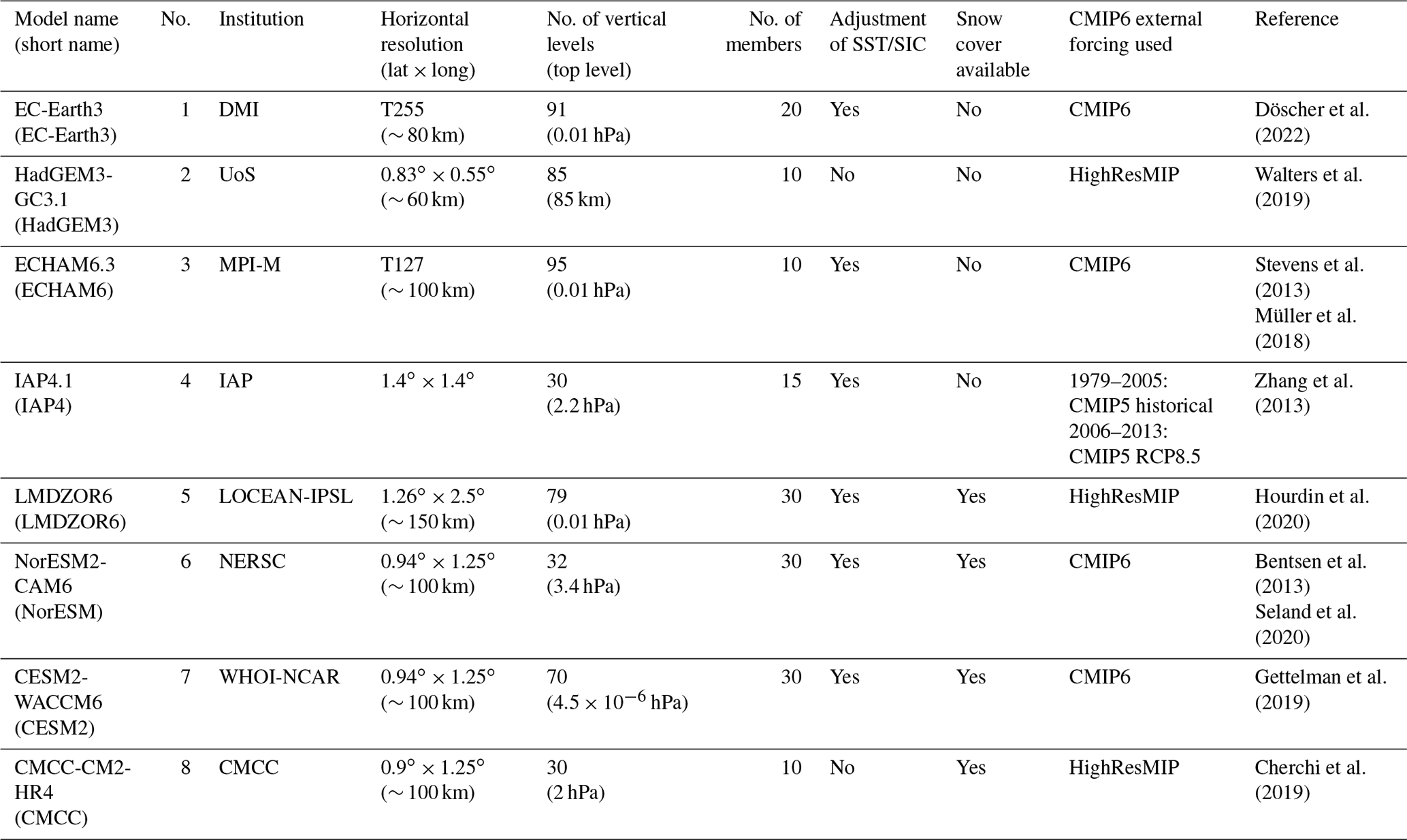
2.2 Model simulations
We use the outputs of the two multi-model land–atmosphere simulation ensembles discussed in Liang et al. (2020, 2021). These simulations used as boundary conditions the SST and SIC provided by the HighResMIP panel of CMIP6 (Haarsma et al., 2016) and atmospheric concentration of aerosol, greenhouse gases, and ozone from CMIP6 (Eyring et al., 2016) in the 1979–2014 period. We use the outputs of eight models wherein the snow depth was saved and distributed (Table 1). The ensemble ALL uses interannually varying daily SST and SIC. The other ensemble, called NoSICvar, is identical but uses a repeated 1979–2014 climatological SIC in the Arctic, with adjustment of the associated local SST (Hurrell et al., 2008). The climate sensitivity to SIC anomalies is provided by the difference of ALL minus NoSICvar. As noted in Liang et al. (2020) and Table 1, the experimental protocol has some small differences for each model, but these deviations are unlikely to affect the results substantially. The number of members varies among models from 10 to 30, while the horizontal resolution varies from about 60 to 150 km. The large diversity of models allows us to study the model dependence. However, for comparison with observations, these ensembles of atmosphere-only models have limitations associated with the lack of active two-way coupling with sea ice and SST, uncertainties in the SST and SIC forcing, and simplified sea ice physics, as discussed in Liang et al. (2021).
We use the monthly SLP, 2 m air temperature, and snow depth in all models. For LMDZOR6 and CMCC, the snow depth was converted into snow water equivalent (SWE) depth, assuming a constant snow density of 240 kg m−3, as found in observations (Sturm et al., 2010). The snow cover is a diagnostic variable in many models and was not available for four models (see Table 1): EC-Earth3, ECHAM6, HadGEM3, and IAP4. Lacking a better formulation, we calculate the snow cover from the SWE using a threshold of 7.5 mm. If the monthly SWE depth is lower (larger) than 7.5 mm, then it is assumed that the snow cover is zero (1). This estimation is based on LMDZOR6, through which we found that a reasonable snow cover extent is obtained with the 7.5 mm threshold when using monthly outputs. This procedure is similar to that of Krinner et al. (2018), except they used a threshold of 5 mm.
The detailed outputs from LMDZOR6 are also used with the monthly geopotential height at 500 and 50 hPa, as well as the daily air temperature. For this model, the wave activity flux from Plumb (1985) is also calculated from daily geopotential height, zonal wind, and meridional wind at 500 and 250 hPa.
All datasets were regridded with bilinear interpolation into the regular grid 1.26∘ × 2.5∘ (∼ 150 km) before analysis. Coastal regions and grid points with complex orography were masked consistently in all models using the observational mask. Multi-model ensemble means (MMMs) are constructed by giving the same weight to each ensemble member, which largely removes the influence of internal atmospheric variability.
2.3 Methods
We study the effects of SST, SIC, and external forcing in driving snow cover anomalies with an analysis of variance (ANOVA) with two factors, also known as two-way ANOVA. The ANOVA is a statistical analysis method for comparing the means of various samples and investigating the influence of one or several categorical independent variables, called factors, on one continuous variable (Storch and Zwiers, 1999). Here the ANOVA is applied in a balanced design to the land snow from the ALL and NoSICvar ensembles, separately for each individual model and for each calendar month. The first factor is the simulated year, called t, which varies from 1979 to 2014. The second factor is the ensemble, called e, and represents the ALL versus NoSICvar ensembles. The interaction between the year and the ensemble is called t:e. In the analysis, the sum of squares quantifies the variance associated with each factor. The ANOVA then compares such variance to the residual variance to test the effect of the factors. The corresponding p value indicates if the effect of the factors (t, e and t:e) is statistically significant. Hereafter, we show such p values, together with the ratio of the sum of squares over the total variance to quantify the variance explained by each factor.
The statistical model of the ANOVA decomposes the snow cover anomalies of a calendar month in each year and ensemble, called X, by
where μ, the theoretical mean of X, corresponds to the seasonal mean of the calendar month. βt is a different constant for each year, βe is a constant for each ensemble, βt:e is an interaction term different for each year and ensemble, and ε is Gaussian noise. If the ANOVA is significant for the factor t, then at least one βt is significantly different from zero. It implies that the time-varying prescribed boundary conditions have an influence on the snow cover in both ALL and NoSICvar, which should result from time-varying SST or external forcings, as they can both influence the atmosphere and land. Similarly, the effect of time-varying SIC is accounted for by the second factor e. If the second factor is significant, with at least one βe different from zero, it demonstrates an influence of varying sea ice concentrations on the land snow. Lastly, if at least one of the interaction terms, βt:e, is significant, it suggests that the influence of SIC is time-dependent. The ANOVA is repeated for each calendar month.
The main drivers of snow cover are characterized using empirical orthogonal functions (EOFs). The EOFs of the Northern Hemisphere snow cover are calculated north of 30∘ N, while the domain for Eurasian snow cover EOFs is 0–180∘ E, 30–90∘ N. Three EOF analyses are performed using the year-to-year time series corresponding to each calendar month separately. The first EOF analysis performed is based on the MMMs calculated from the ALL experiments. The EOF pattern is denoted as EOFBC, where BC stands for boundary conditions and indicates the driving effect of the prescribed SST, SIC, and external forcings (concentration of greenhouse gases, aerosols, and ozone). As the forcing from sea ice concentration is weak (Liang et al., 2021), the EOFs are almost identical when using NoSICvar instead of ALL. For instance, the pattern correlation between the first EOFBC (EOF1BC) of ALL and that of NoSICvar is 0.95, 0.93, and 0.98 for November, January, and April, respectively. EOF1BC therefore mainly quantifies the SST and external forcing. The corresponding principal components (PCs) are denoted PCBC. A second EOF analysis, called EOFSIC, is identical but performed on the difference between the MMM of ALL and NoSICvar to highlight the effect of the SIC variability. The corresponding principal components (PCs) are denoted PCSIC.
Hereafter, all principal components are standardized, and the EOFs are illustrated using their regression onto the standardized PC. The sign convention is that a positive PC corresponds to an EOF with positive loading over eastern Europe (20–70∘ E, 55–70∘ N).
Lastly, the internal land–atmosphere variability is investigated in the model simulations with a third EOF analysis. The internal variability is investigated after removing the ensemble mean of the snow evolution that mostly reflects the effect of SST, SIC, and external forcing. We conduct an EOF analysis separately for each model using all the members of ALL and NoSICvar concatenated after the removal of their respective ensemble means. This third analysis provides EOFInt and PCInt as spatial patterns and time series, respectively. The relevance of this analysis might be limited when the ensemble size is small (only 10 members for some models), as the ensemble means are more affected by internal variability.
In addition, various fields, such as the surface air temperature, SLP, geopotential height, and zonal wind, are regressed onto PCBC, PCSIC, and PCInt. The p values of the univariate regression slopes are given by a Student's t test. The year-to-year autocorrelations for separate calendar months are typically insignificant between 0 and 0.05 (not shown). The only exception is for April, when such autocorrelation is significant over Scandinavia and the East European Plain, but it remains modest with maximum values at 0.08. Hence, we did not account for a reduction in the degree of freedom due to year-to-year correlation.
The ANOVA, the retrieval of EOFInt, and the regression analyses using PCInt are performed separately for each model, but the figures provide the mean for the eight models using a weight proportional to the ensemble size of each model ensemble, referred to as the multi-model mean (MMM). This avoids giving too much weight to models with only 10 ensemble members. We indicate grid points where the sign of anomalies is the same in seven models out of eight. This corresponds to a probability of 6.2 % when considering that the sign of the anomaly has a probability of 50 % in the models, as deduced for the binomial probability distribution. We also indicate the grid points where the p value is below 5 % in at least five models out of eight.
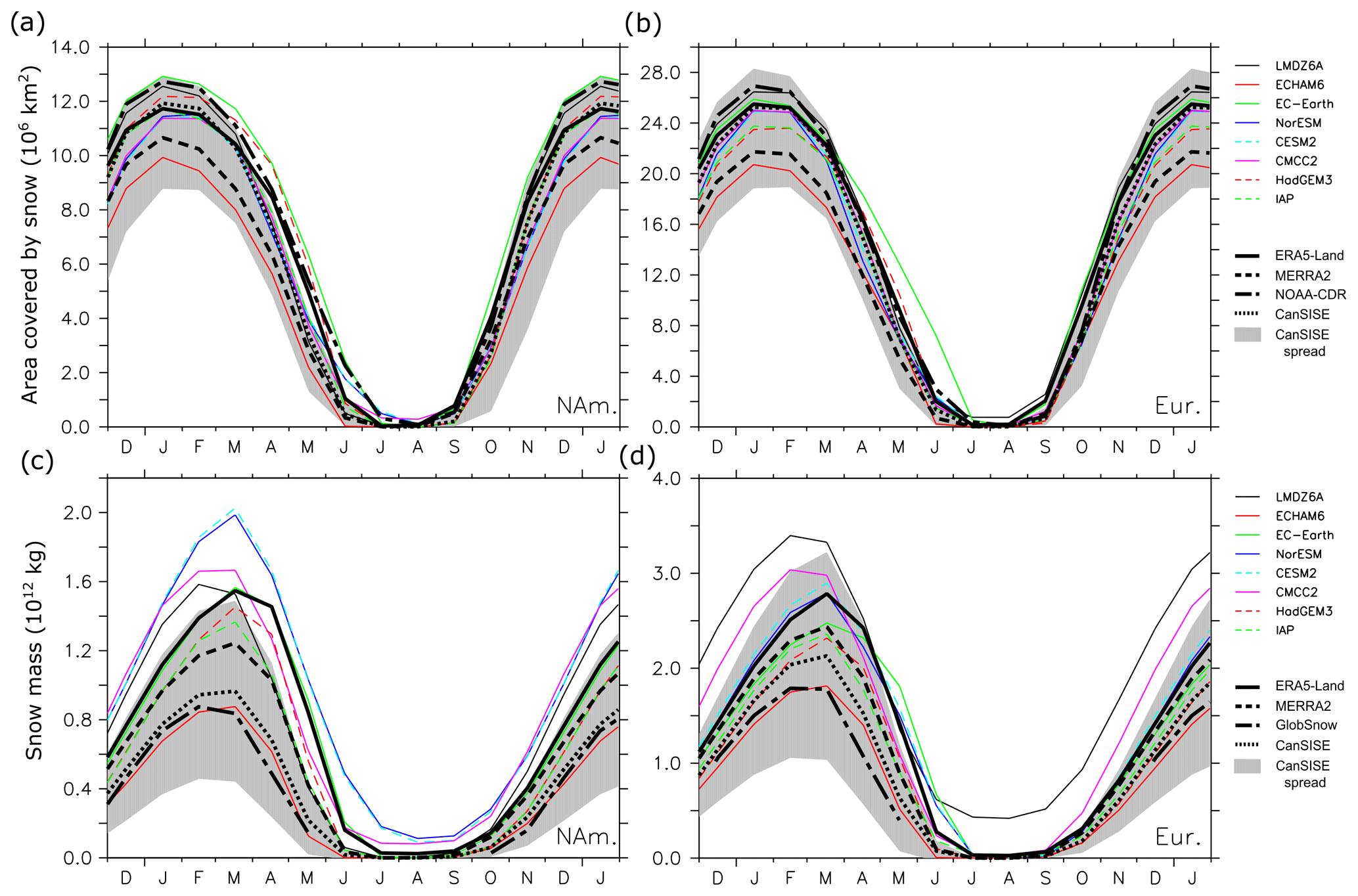
Figure 1(a, b) Seasonal cycle of the area covered by snow, in 106 km2, in (a) North America and (b) Eurasia. (c, d) Seasonal cycle of the Northern Hemisphere snow mass, in 1012 kg, in (c) North America and (d) Eurasia. Color curves show results from models. Thick black curves show analyses or reanalyses. The gray shading provides the observational spread obtained from CanSISE.
3.1 Climatology
First, we briefly assess the Northern Hemisphere land snow simulated in the eight models. The mean seasonal cycle of land snow extent and snow mass is first calculated over North America and Eurasia in 1979–2014. The snow extent over North America (0–90∘ N, 180∘ W–0∘ E) and Eurasia (0–90∘ N, 0–180∘ E) has a maximum in January–February (Fig. 1a and b, black lines). November and April are associated with the start and the end of the season with extensive land snow coverage, respectively. The seasonal cycle of the Eurasian snow area is well represented by all the models (Fig. 1b, color lines). The differences between the models are within the range of uncertainty between the observational datasets, except for EC-Earth3 that simulates a slower snow cover decrease in spring. The snow cover area over North America (Fig. 1a) is also well captured by models, but it is overestimated in EC-Earth3 and underestimated by ECHAM6. We also calculate the standard deviation obtained from year-to-year time series for each month. The interannual variability in models also agrees with that found in observations (Fig. S1 in the Supplement).
There is less agreement on the snow mass (Fig. 1c and d). First, the snow mass estimations from observations show a large spread that is maximum from February to May. Then, LMDZOR6 and CMCC both overestimate the snow mass in Eurasia and North America from December to March. NorESM and CESM2 only overestimate the snow mass over North America, especially from February to March. Other models simulate snow masses within the spread of observational products. In conclusion, the models reproduce the observed snow cover seasonality but tend to overestimate the snow mass. These conclusions are in agreement with the similar analysis of CMIP6 AOGCMs from Mudryk et al. (2020) and Zhong et al. (2022). Therefore, the use of atmosphere-only simulations does not significantly reduce the land snow biases compared to AOGCM simulations.

Figure 2(a) Mean January snow cover in CanSISE, in fraction. (b–i) Mean snow cover (color shading) bias in January, in fraction, calculated as the ALL ensemble mean minus CanSISE for each model. The contours indicate the mean snow cover fraction in CanSISE (contour interval 0.2) shown in (a).
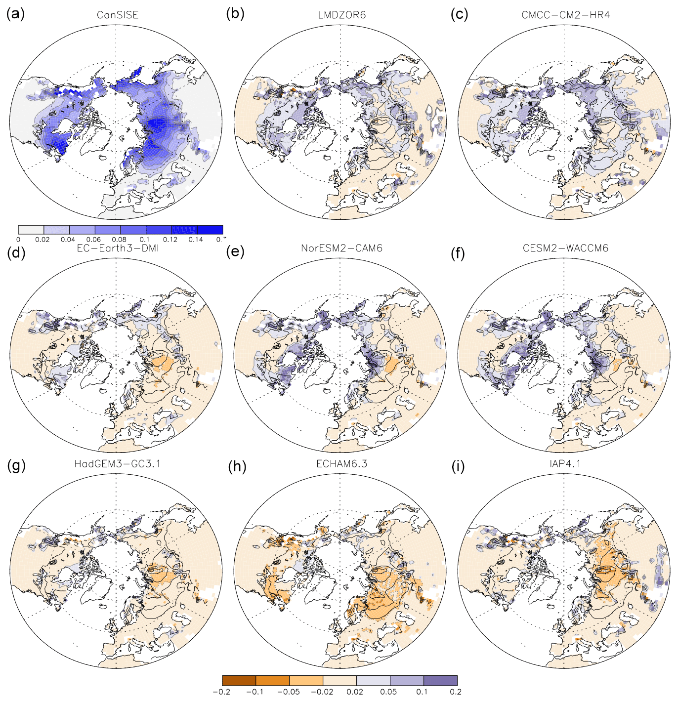
Figure 3Same as Fig. 2, but for the snow water equivalent (in meters).
The location of the snow cover biases of each model compared to CanSISE is illustrated for January in Fig. 2. We chose CanSISE as a reference as it is based on an ensemble of observations. Most models simulate more snow cover than observational products from the Tibetan plateau to eastern Siberia and too little snow cover over southwestern Eurasia. No apparent snow biases are found over the fully snow-covered domain between eastern Europe and central Asia. Over North America, there is generally more snow in models than in observations over the Rocky Mountains, and a few models also underestimate the snow cover over northeastern Canada. Given the large uncertainty of the observational products over mountain regions, more observations would be needed to fully confirm the biases over these regions. The snow water equivalent in models (Fig. 3) shows a generally positive bias over land with no consistent large-scale pattern in LMDZOR6, CMCC, NorESM, and CESM2. The bias is negative in ECHAM6 and IAP4.1, with an underestimation of the SWE over the East European Plain and northeastern Siberia, respectively. EC-Earth3 and HadGEM3 agree with the observations.
Hereafter, we focus on the land snow variability in November, January, and April, which represent the start, the maximum, and the end of the period with large snow coverage in the Northern Hemisphere (Fig. 1).
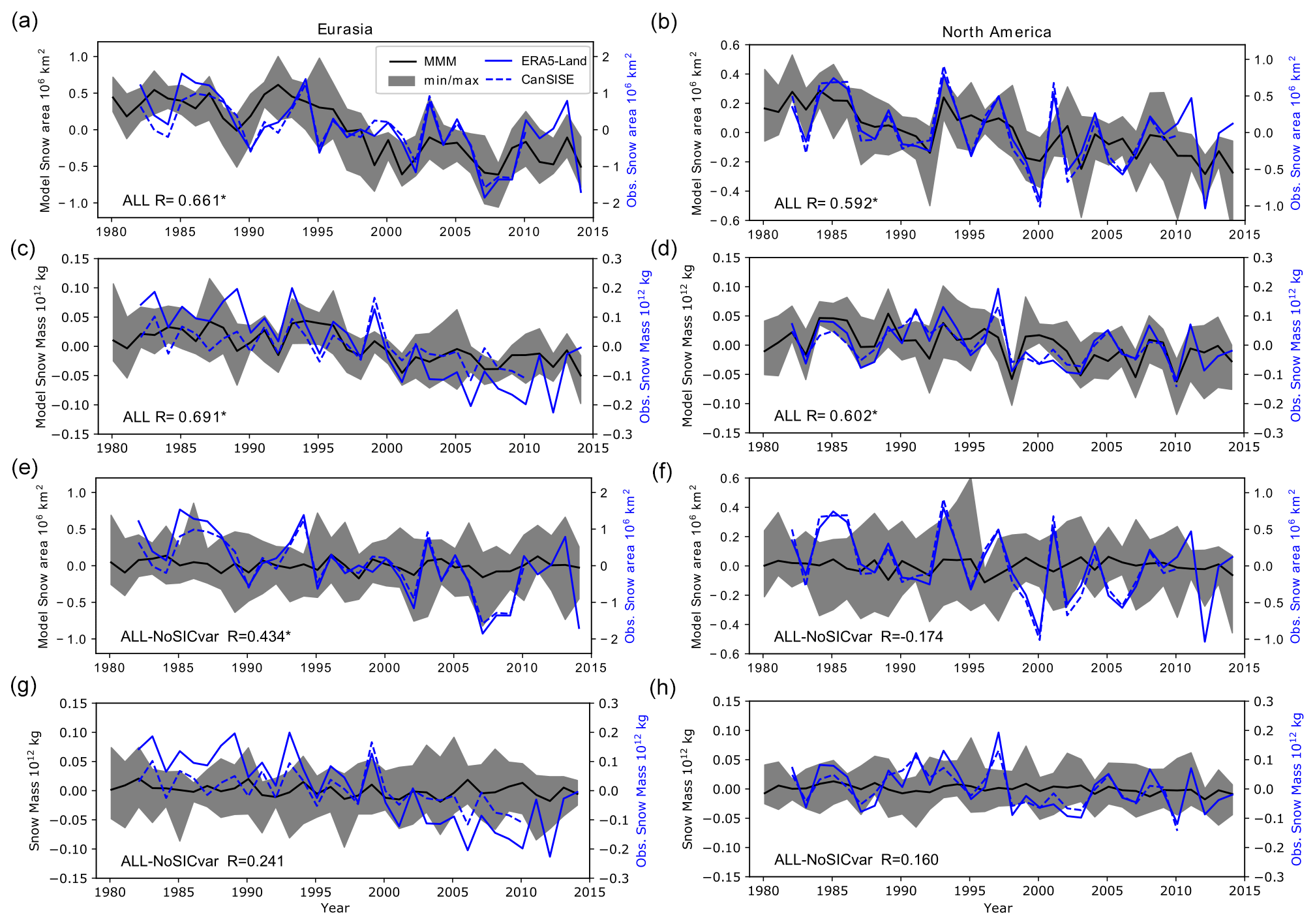
Figure 4Time series of the anomalous area covered by snow in 106 km2 (a, b) and anomalous snow mass in 1012 kg (c, d) in winter (from November to April) in (b, d, f, h) North America and (a, c, e, g) Eurasia in observations and the simulation ALL. (e, f) Same as the first row, but for ALL minus NoSICvar. (g, h) Same as the second row, but for the difference of ALL minus NoSICvar. Note the different scale on the y axis for (left axis, black line) models and (right axis, blue line) ERA5-Land and CanSISE observations. The gray shading indicates the range between the minimum and the maximum values among the eight models. The black curve is the multi-model ensemble mean. The correlation between the multi-model mean and ERA5-Land is given in the bottom left corner of each panel, with the star symbol indicating a p value below 5 %.
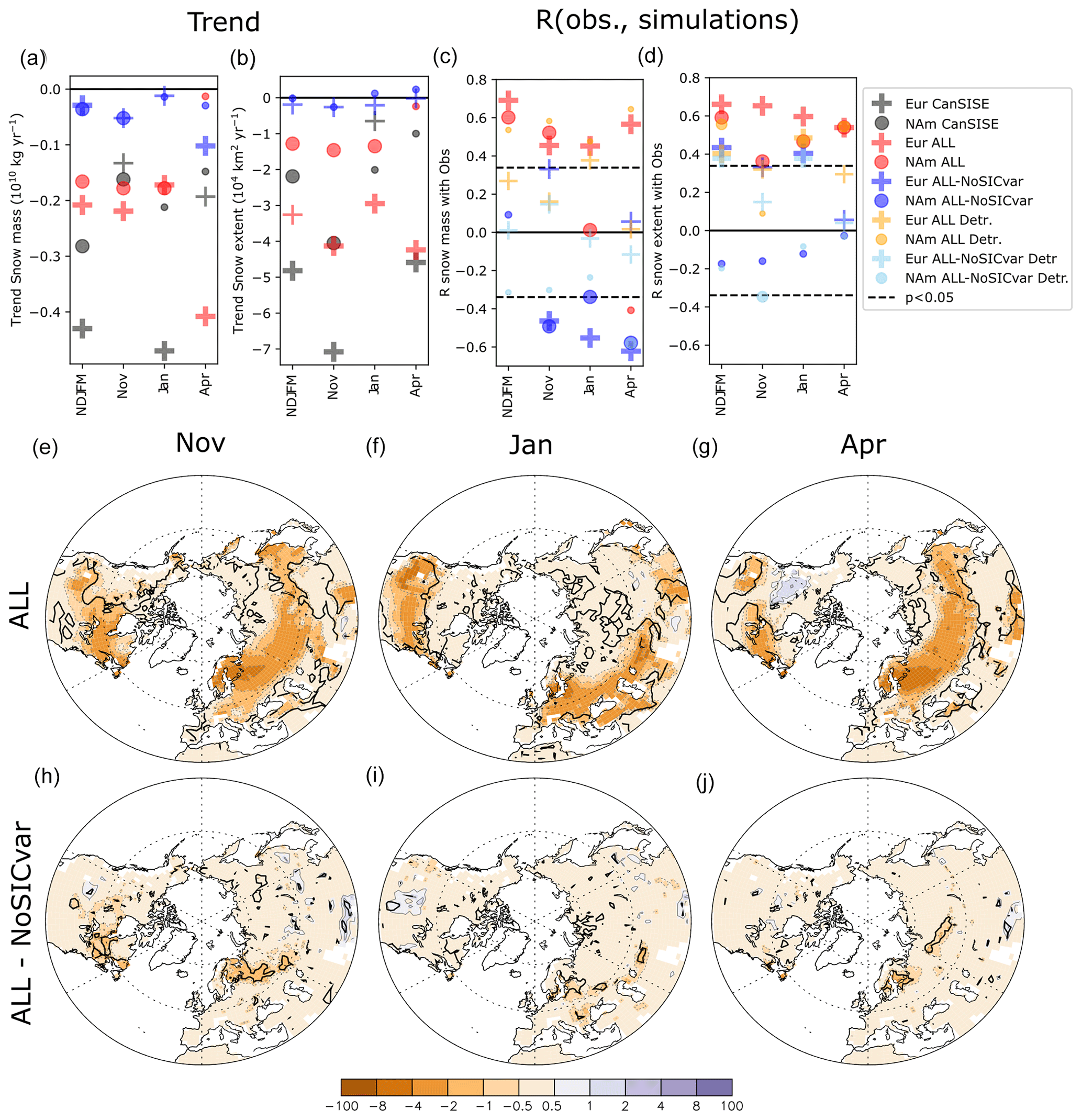
Figure 5Trend in Northern Hemisphere (a) snow mass and (b) snow extent. Correlation between ERA5-Land and simulated values for (c) snow mass and (d) snow extent. The red (blue) symbol denotes the simulation ALL (ALL minus NoSICvar) for 1979–2014. The gray symbol denotes the CanSISE observations for 1979–2010. The orange (blue sky) symbol is for the simulation ALL (ALL minus NoSICvar) when using linearly detrended fields. Northern Hemisphere trend in snow cover (in percent per decade) for the multi-model mean of the simulations (e–g) ALL and (h–j) the difference of ALL minus NoSICvar in (e, h) November, (f, i) January, and (g, j) April. In (a–d), the size of the symbol is large (small) if the significance of the trends is below (above) 5 %. In (e–j), black contours indicate where the p values are lower than 5 %.
3.2 Assessment of snow cover anomalies
Figure 4a and b show the time series of the anomalous snow cover area in winter, defined by the average from November to March, in the MMM of ALL. The anomalies are defined with respect to the 1979–2014 climatology. The observational values are also shown but using a different scale to facilitate the comparison. Indeed, the decreasing trend of the MMM snow cover area is roughly half of that observed over Eurasia and North America (see also red and gray symbols in Fig. 5b). In addition, the year-to-year variability of ALL is much smaller than that observed. This presumably reflects the fact that the observations correspond to one realization, while the model ensemble means are averaged over 10 to 30 members, depending on the model, which strongly reduces the impact of internal variability. This suggests that either half of the observed trends is due to internal variability or that the influence of SST or external forcing is underestimated by half in the models. Similar results are found for the snow mass, but the decreasing trend over Eurasia is much weaker in models than in observations (Figs. 4c, d, and 5a). The timings of some of the minima and maxima are consistent, as in 2007–2008 for the snow extent over Eurasia (Fig. 4a), in 1993 and 1999–2000 for the snow extent over North America (Fig. 4b), and in 1987, 1998, and 2010 for the North American snow mass (Fig. 4d). This is consistent with the strong relationship between El Niño events and positive phases of the Pacific–North American (PNA) pattern, which are associated with warm anomalies and decreasing snow depth over western North America (Ge and Gong, 2009).
The correlation between the ALL MMM and ERA5-Land snow cover area is 0.66 (0.59) over Eurasia (North America), while it is 0.69 (0.60) over Eurasia (North America) for snow mass, which demonstrates a dominant influence of the boundary conditions. After removing the linear trend from every time series, the correlations are smaller, but they remain significant, except for snow mass over Eurasia (compare red and yellow symbols in Fig. 5d).
The overall impact of the sea ice variations on the snow cover area and snow mass is limited, as shown by the differences between the MMM of ALL and NoSICvar over North America (Fig. 4f–h). The time series in Fig. 4f–h show no clear trend and are not significantly related to observations at the 5 % level (Fig. 5d), except for the Eurasian snow extent (Fig. 4e), which is significantly correlated with observations (R = 0.43) even for detrended time series (R = 0.38).
The correlations of land snow area and mass between observation and models remain significant over Eurasia and North America separately for November, January, and April in Fig. 5c and d for ALL (red and orange symbols), which confirms the robust influence of boundary conditions. The 1980–2014 linear trends of snow cover and snow depth are also assessed in Fig. 5a and b using the MMMs and calculating their statistical significance with a Student's t test, as detailed in Liang et al. (2021).
Over Eurasia and North America, the trends in ALL for November and January (Fig. 5a and b, red circle and plus) are consistent with that of the whole winter (NDJFM). However, in April, the snow depth trend over Eurasia in ALL is more negative, while the snow extent trend over North America is smaller and insignificant. The comparison between the observed CanSISE (Fig. 5a and b, gray circle and plus) and simulated trend reveals important differences, as a dominant negative trend is observed in November and January for snow extent and mass, respectively. A comparison of the trends obtained in other observational datasets (Figs. S2 and S3) shows a large spread in trend estimates, with increasing snow extent in fall and early winter in the NOAA-CDR observations, while ERA5-Land, MERRA-2, and CanSISE show a decreasing snow extent, as found previously (Brown and Derksen, 2013; Mudryck et al., 2017). The reason for this difference between the NOAA-CDR and multi-observation products is unknown (Mudryck et al., 2017). This suggests that observational uncertainties are important, especially in fall, as reported by Fox-Kemper et al. (2021). The trend maps obtained from ALL MMM in November, January, and April (Fig. 5e–g) reveal an important large-scale decrease in snow cover, which is maximum at the edges of the snow-covered domain.
The influence of sea ice is investigated with the trends of the MMM of ALL minus NoSICvar and the correlation between observations and the MMM of ALL minus NoSICvar in Fig. 5a–d (blue and sky-blue symbols). The trends of ALL minus NoSICvar are negative and significant for snow mass only, which may reflect an influence of the sea ice loss reducing the snow mass. For the snow cover, the correlation and trend are mainly small and insignificant. The trend maps (Fig. 5h–j) show a weak but significant decreasing trend for January and April in southern Scandinavia extending eastward into Eurasia. In November, a decreasing trend is located east of Scandinavia, downstream of the Barents Sea. Such a location is in agreement with the large oceanic heat release expected from the observed Barents–Kara sea ice loss (Deser et al., 2015). Another decreasing snow cover trend is also simulated over northeastern Canada in November.
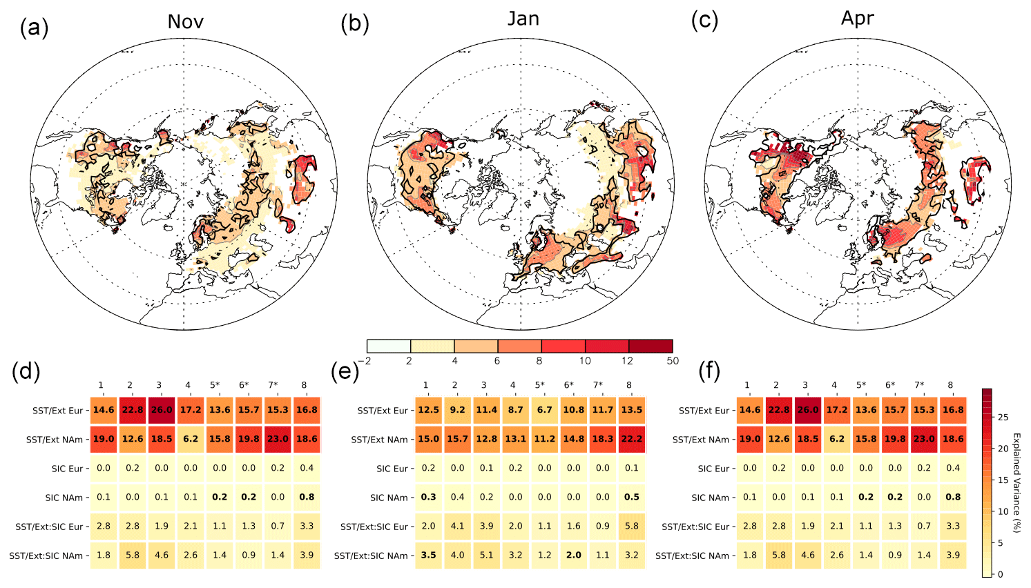
Figure 6Variance fraction (in %) of the interannual snow cover anomalies explained by SST, external forcing, and sea ice concentration for (a) November, (b) January, and (c) April. The thick black curve indicates where the p value of the ANOVA test is lower than 5 % for at least five models out of eight. Variance fraction (in %) of the snow cover area over Eurasia (Eur) and North America (NAm) calculated for each model separately for (d) November, (e) January, and (f) April. The numbers from 1 to 8 designate the model (see Table 1 for correspondence with model name). The star symbol indicates when 30 members are available for both ALL and NoSICvar. The factor t, representing the influence of SST and external forcings, is referred to as SST/ext. The factor e, representing the influence of SIC on the time mean snow, is referred to as SIC. The factor t:e, representing the influence of SIC on the time-varying snow, is referred to as SST/ext:SIC. Numbers are given in bold font if the ANOVA test has a p value below 5 %.
3.3 Role of the boundary conditions in driving snow cover
The influence of boundary conditions is quantified using an ANOVA (see Sect. 2.3). We first applied the ANOVA separately at each grid point. The effect of SST and external forcing represented by the factor t is found to be dominant. The snow cover variance fraction associated with this factor is significant in all models in November, January, and April (Fig. 6a–c). It is largest over the midlatitude edges of the snow cover in Eurasia or North America and may reach 15 % over the Tibetan plateau, although models and observations have large uncertainties there (Mudryk et al., 2020). A large variance fraction (> 5 %) is also simulated over the Rockies and Scandinavia. In November, the variance fraction is ∼ 4 % to 5 % over northern Canada and a latitudinal band from Scandinavia to eastern Siberia. By January, the variance fraction at the edge of the snow cover domain increases on average to ∼ 6 % and shifts toward eastern Europe and from the Caspian Sea to eastern China. In April, the large variance fraction is more important (∼ 6 %–10 %) but more localized from the East European Plain to southern Siberia and over northern Canada. The results are summarized by an ANOVA using the Eurasia or North America snow area instead of grid point values in Fig. 6d–f. Models show a significant influence of SST and external forcing (indicated by SST/ext in Fig. 6d–f) with 10 % to 25 % of the variance explained over both domains, despite important differences between models.
The snow cover variance associated with the varying sea ice concentration is given by the factors e and t:e (see Sect. 2.3 for details) representing the influence of the SIC on the time mean and time-varying snow, respectively. The variance fractions show no clear agreement between models and are largely insignificant at most grid points (not shown). The results are summarized in Fig. 6d–f for the snow cover area over Eurasia and northern America. The sea ice only explains 1 % to 5 % of the variance, as found in the interaction t:e, and the impact on the time mean snow cover is below 0.3 % in most models. In most models, the ANOVA test is not significant for these two factors. We conclude that sea ice does not have a robust influence on the snow cover in our simulations. Using SWE instead of snow cover yields similar results (not shown).
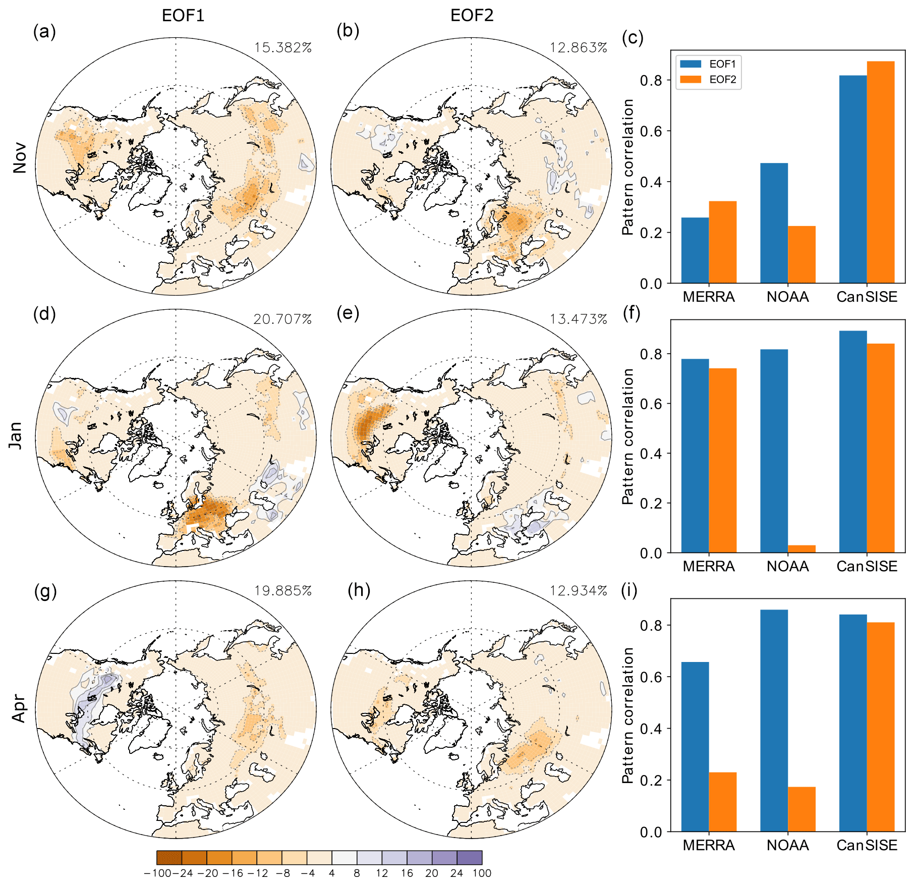
Figure 7(a, d, and g) First and (b, e, and h) second EOFs (in %) of Northern Hemisphere snow cover anomalies in ERA5-Land during 1981–2014 for (a–c) November, (d–f) January, and (g–i) April. The variance explained by the EOFs is indicated. (c, f, and i) Pattern correlation between the (blue bar) EOF1 and (orange bar) EOF2 of ERA5-Land and that found in the other observational datasets MERRA-2, NOAA-CDR, and CanSISE.
3.4 Assessment of the role of the boundary conditions for snow cover
To assess the main patterns of simulated year-to-year snow cover variability, we first investigate analyses or reanalyses, with separate EOFs (north of 30∘ N) for each calendar month. Figure 7 shows the first two snow cover EOFs in ERA5-Land in, from top to bottom, November, January, and April, as well as their pattern correlation with the corresponding EOFs obtained from the three other observational datasets (right). In November, the first EOF (EOF1) shows anomalies of the same sign with large loading over the East European Plain, eastern Eurasia, and central North America, near the edges of the mean snow-covered area. The second EOF (EOF2) is a dipolar pattern with large loading over eastern Europe and small loading with the opposite sign between the Aral Sea and Lake Baikal and in western North America. In January, EOF1 is dominated by a large loading over Europe, while EOF2 is dominated by strong anomalies over North America. In addition, EOF1 and EOF2 display small anomalies near the edge of the Eurasian snow-covered domain. In April, EOF1 is a dipole with large loading over North America and anomalies with an opposite sign between the Caspian Sea and Lake Baikal. EOF2 only shows large loading over the East European Plain. CanSISE provides very similar snow cover EOFs as ERA5-Land in all months. The EOF1 patterns in MERRA-2 and NOAA-CDR are also similar in January and April, but they are different in November. The EOF2 patterns in MERRA-2 and NOAA-CDR mainly disagree with ERA5-Land. This suggests that the observational uncertainty is large in November but that the EOF1 pattern is otherwise rather robust.
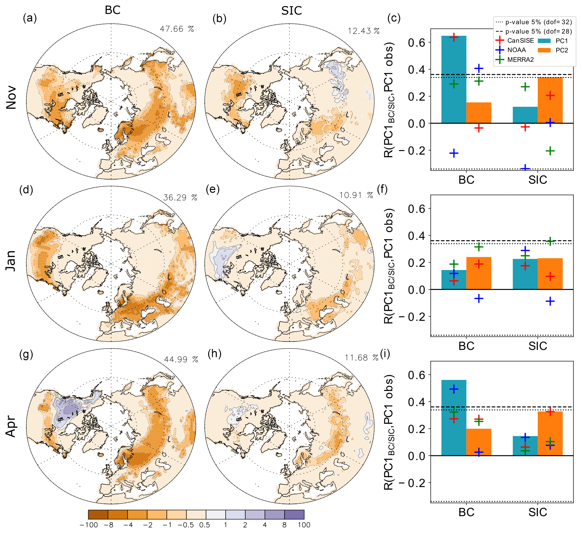
Figure 8(a, d, and g) First EOFBC of the snow cover anomalies (in %) associated with sea surface temperature and external forcing anomalies and (b, e, and h) first EOFSIC (in %) associated with sea ice concentration anomalies for (a–c) November, (d–f) January, and (g–i) April. (c, f, and i) Correlation between the observed snow cover PC1/2 and PC1BC and between the observed PC1/2 and PC1SIC when using (blue and orange bars) ERA5-Land, (green cross) MERRA-2, (blue cross) NOAA-CDR, and (red cross) CanSISE. The blue (orange) bars and the associated crosses provide the results when using PC1 (PC2) from observations. The dashed line provides the 5 % level of statistical significance for the correlation when using ERA5-Land, MERRA-2, or NOAA-CDR in 1981-2014 (32 degrees of freedom). The dotted line is the same as the dashed line but when using CanSISE in 1981-2010 (28 degrees of freedom).
To emphasize the role of external forcing, SST, and SIC for the simulated snow cover, the first EOF of the Northern Hemisphere snow cover in the MMM of ALL, called EOF1BC, is shown in Fig. 8a, d, and g. The corresponding principal components, hereafter PC1BC, all show a positive trend (not shown) so that the EOF1BC resembles the maps of the land snow trend from ALL in 1981–2014 (compare Figs. 5e–g and 8a, d, g). November EOF1BC (Fig. 8a) also shows anomalies of the same sign over North America and from Scandinavia to eastern Siberia, at the edges of the mean snow-covered region, and near the Tibetan plateau. In January (Fig. 8d), the pattern is again a monopole, but it is centered over a band from Europe to East Asia as the snow-covered domain is broader than in November. In April (Fig. 8g), the loading over Eurasia is similar to that found in November, but the anomalies over North America are opposite. EOF1BC explains 36 % to 48 % of the variance in November, January, and April.
The EOF associated with the boundary conditions and external forcings can be compared with the observed snow cover EOF. The first two EOFs in ERA5-Land (Fig. 7, left) have some similarities to the EOF1BC patterns in Fig. 8a, d, and g. However, the loading is more localized in ERA5-Land, without a clear location at the edge of the snow-covered domain. Moreover, in ERA5-Land EOF1 (EOF2) only explains 15 % to 21 % (12 % to 13 %) of the variance. The somewhat different patterns and the smaller explained variance may reflect in part the large influence of internal atmospheric variability in observations. To reveal the links between the observed snow cover variability and the influence of SST and external forcing, PC1BC is compared to the observed snow cover PC1 and PC2. The correlation between PC1BC and the observed PC1 (Fig. 8c, f, and i, left, blue bars) is only significant when using ERA5-Land and CanSISE in November and when using ERA-Land and NOAA-CDR in April, and it is not significant at all in January. Moreover, the correlation between PC1BC and the observed PC2 (orange bars) is only 5 % significant in November for NOAA-CDR. After removing a linear trend from all the time series (not shown), the correlations with PC1BC that largely stem from SST forcing are smaller, and they only remain significant with ERA5-Land PC1 in November (R = 0.36) and with ERA5-Land (R = 0.47) and NOAA-CDR (R = 0.48) PC1 in April. This confirms the larger effect of changing SST and external forcing in November and April, although the EOF analysis is not robust among the observational datasets. There is no significant correlation in January, presumably because the internal variability is larger.
The snow cover EOFs solely related to the sea ice are calculated from the MMM difference of ALL minus NoSICvar (Fig. 8b, e, and h). The variance fraction explained by the first EOFSIC is between 10 % and 13 %. The absolute variance explained by EOFSIC (not shown) is 6 to 13 times smaller than the one explained by EOF1BC, which confirms that sea ice has a much smaller influence than SST or external forcing. In November, EOF1SIC is a dipole with the same sign between the East European Plain and North America and an opposite sign over eastern Siberia. In January, EOF1SIC is a dipole with the opposite signs between North America and Eurasia. The pattern in April is reminiscent of EOF1BC, but with smaller anomalies. EOF1SIC can hardly be related to the observed snow cover variability, as the correlations between PC1SIC and the observed PCs are weak. This confirms that the sea ice cover has little or no impact.
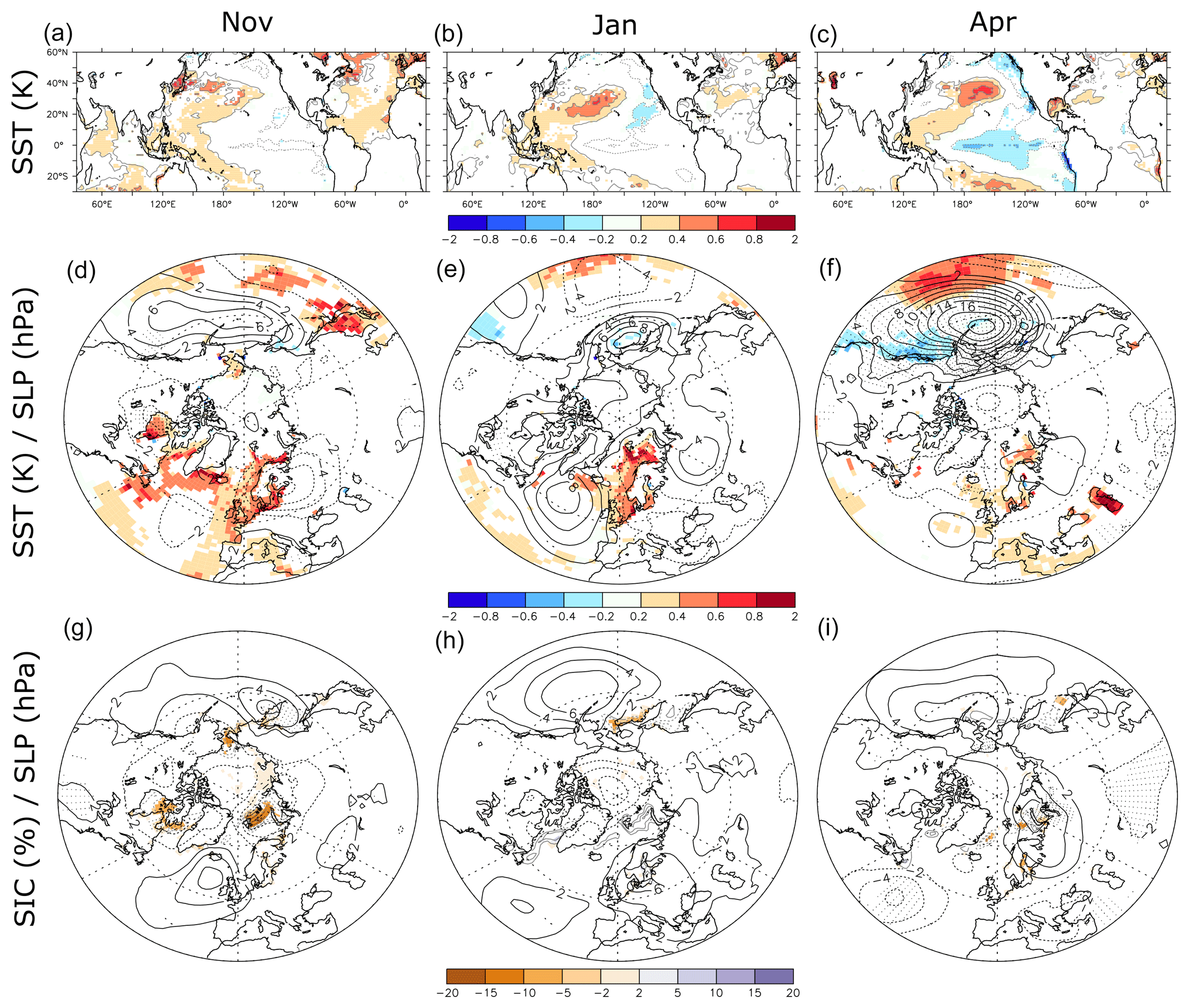
Figure 9(a–c) Regression of the SST (∘C) (gray contours and color shading) on PC1BC. (d–f) Regression of the SST (∘C) (color shading) and sea level pressure (hPa) (black contour, contour interval 2 hPa; dotted contours for negative values) on PC1BC. (g–i) Regression of the SIC (%) (gray contours and color shading) and sea level pressure (hPa) on PC1SIC (black contour, contour interval 2 hPa; dotted contours for negative values). In all panels, color shading indicates a p value below 5 % for the regression of the SST or SIC. Dots indicate p values below 5 % for the SLP regression in panels (d–i). Left panels (a, d, and g) are for November. Center panels (b, e, and h) are for January. Right panels (c, f, and i) are for April.
The SSTs related to the snow cover changes are given by the regression of the SST anomalies from ALL onto PC1BC. The regressions can be interpreted as the SST patterns contributing to the snow cover anomalies of EOF1BC or the SST pattern responding to the external forcing that affected the snow cover changes. We note warm SST anomalies in the western equatorial Pacific and the central midlatitude North Pacific in all months (Fig. 9a–c), consistent with the extended negative snow cover anomalies of EOF1BC (Fig. 8a, d, and g). This might reflect the SST trends observed during that period, which were found to result from the combination of external forcing superimposed on the changes in the Pacific decadal variability (Dai and Bloecker, 2018; Gastineau et al., 2019). In April, there is a cold anomaly in the central and eastern equatorial Pacific, with an extension toward the eastern North Pacific. This horseshoe pattern resembles a La Niña pattern and its extension toward midlatitudes, called the Interdecadal Pacific Oscillation (Newman et al., 2016). We also note warm SST anomalies over the North Atlantic in November, which remain similar, but with smaller amplitude, when removing the linear trends (not shown), suggesting a role of interannual or decadal North Atlantic variability.
To understand these links, the SLP anomalies in ALL MMM associated with PC1BC are shown in Fig. 9d–f. In April, the SST is associated with a weakened Aleutian Low in the North Pacific and a PNA pattern, which are consistent with the expected pattern associated with cold equatorial Pacific SST anomalies. The weakened Aleutian Low leads to cold air advection over western North America, which explains the positive snow cover anomalies in that region (Fig. 8g). Therefore, the SST over the Pacific Ocean plays a significant role in the April snow cover over North America. The SLP anomalies are otherwise not significant for November and January. We also note positive SST anomalies in the Atlantic and Pacific oceans, which might reflect the positive SST trend observed during that period at those locations.
To investigate the role of sea-ice-driven variability, we calculated the regression onto the PC1SIC index, using the prescribed SIC in ALL, and the MMM difference of SLP from ALL minus NoSICvar. PC1SIC has a decreasing trend in November (not shown), and it reflects small but significant negative SIC anomalies in the Barents, Labrador, and Bering seas (Fig. 9g). In November, the SLP anomaly is negative over the negative sea ice anomalies, as expected from the warming in the atmospheric planetary boundary layer, as shown in previous studies (Peings and Magnusdottir, 2014; Liang et al., 2021). The November SLP pattern (Fig. 9g) is different from a negative North Atlantic Oscillation (NAO) or a Ural blocking pattern as previously found as a response to sea ice loss (Mori et al., 2014; Kug et al., 2015; Nakamura et al., 2015; King et al., 2016; Smith et al., 2022), but it is consistent with previous studies using atmosphere-only experiments (Ogawa et al., 2018; Liang et al., 2021). In January and April, the sea ice anomalies are very small. In January, the SLP pattern is insignificant, but in April, there is a cyclonic anomaly around 50∘ N over the Atlantic Ocean, a small cyclonic anomaly over the Mongolian Plateau, and a weakening of the Aleutian Low. Positive SLP anomalies are also located over the Kara Sea, but these anomalies cannot be linked to the snow cover anomaly in a simple way. In all cases, removing the linear trends leads to different results (not shown), so the relationships shown in Fig. 9g–i mostly reflect the impact of the sea ice declining trend.
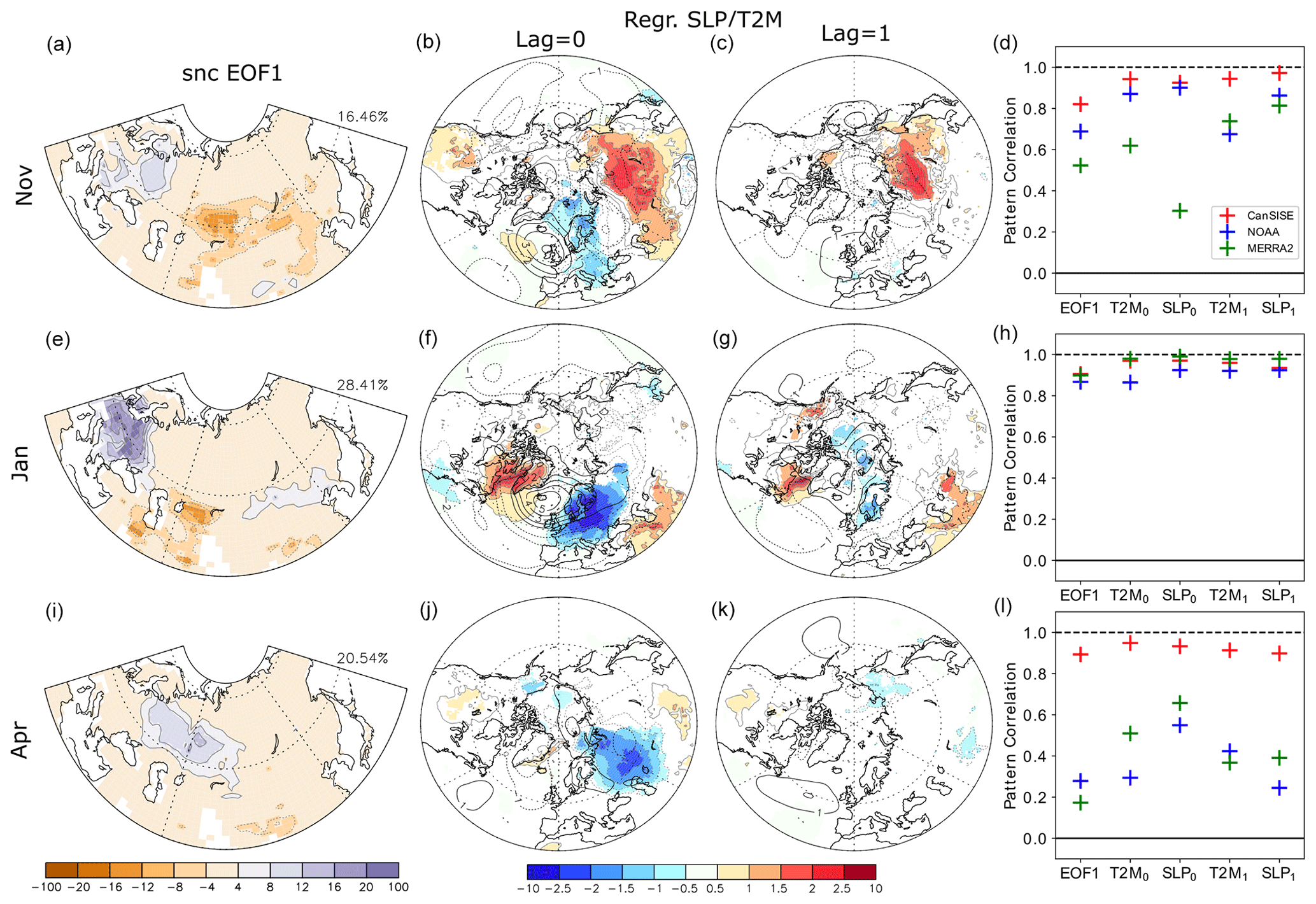
Figure 10First EOF (first column from left; a, e, and i) of the detrended Eurasian snow cover in ERA5-Land, shown as the regression of the snow cover, in %, onto the first PC. Regression (second column; b, f, and j) of the observed (color shading and gray contours) surface air temperature, in ∘C, and (black contour; contour interval 1 hPa) sea level pressure in hPa on PC1 at lag = 0, and (third column; c, g and k) at lag 1, i.e., for PC1 leading the atmospheric fields by 1 month. Pattern correlation (fourth column; d, h, and l) of the EOF1s and of the regressions of surface air temperature or sea level pressure on the Eurasian snow cover PC1 between ERA-Land and other snow cover datasets. T2M0 and SLP0 designate the pattern correlation of the regressions at lag = 0; T2M1 and SLP1 designate the pattern correlation at lag 1. The first row (a–d) is for November, the second row (e–h) for January and the third row (i–l) for April. In the second and third columns, color shading indicates p value below 5 % for the surface air temperature regression.
4.1 Internal variability of snow cover
The impact of internal atmospheric variability on snow cover anomalies is investigated over Eurasia. We focus on Eurasia as it is the largest continent, and snow cover was previously suggested to influence the Northern Hemisphere atmospheric circulation (Cohen and Entekhabi, 1999; Cohen et al., 2014; Gastineau et al., 2017). In the observational datasets, we remove a quadratic trend from all variables, which should remove a large part of the changes linked to the long-term evolution of external forcing, and then quantify the internal variability, which is largely due to atmosphere–land processes, in addition to a residual influence of SST and SIC. The first EOF of the detrended snow cover in ERA5-Land is shown in Fig. 10a, e, and i. The patterns are somewhat similar to those obtained over the Northern Hemisphere before detrending (Fig. 7), but the EOF1 over Eurasia in November and April corresponds to the EOF2 of the Northern Hemisphere before detrending. The similarity in the EOF1 pattern obtained in January in models and observations (Figs. 7d and 10e) suggests that internal variability is dominant during that month, as opposed to November and April when forcings are important. The regressions of the SLP and surface air temperature (Fig. 10b, f, and j) onto the PC1 at no lag illustrate the influence of the NAO on the snow cover in January, with cold air advection increasing the European snow cover. In November and April, the snow cover is linked to a trough over the Ural region, with cold (warm) air advection over its western (eastern) flank. The trough over central Eurasia is part of a wave-like perturbation between the Atlantic Ocean and Eurasia. In November, the trough extends to eastern Siberia and is associated with a warming and a snow cover decrease in central Siberia. These patterns are similar in January when using the other three snow cover datasets (see Fig. 10d and h). In November, the patterns remain similar except for MERRA-2. In April, the patterns are different (Fig. 10i) and the SLP anomalies are smaller (Fig. 10j).
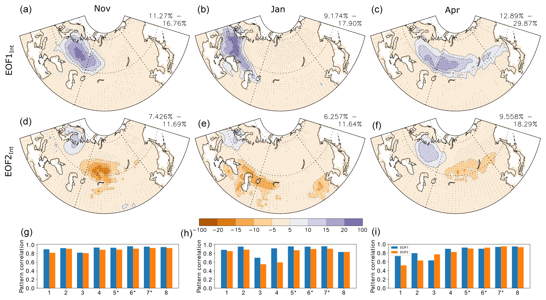
Figure 11 First (first row, a–c) and (second row, d–f) second EOFInt of the Eurasian snow cover (in %) associated with internal atmospheric variability in the simulations ALL and NoSICvar. The patterns are the average patterns of the eight models. The numbers displayed on top are the minimum and maximum variance explained by that EOF among the eight models. Dots indicate the locations where seven models out of eight have EOFInt anomalies with the same sign. Spatial pattern correlation(last row, g–i) between the EOFInt obtained from each model and that of the model average. The blue (orange) bar shows the results when using the first (second) EOF. The numbers on the x axis designate each model (see Table 1 for the corresponding model names). The symbol star indicates when 30 members are available for both ALL and NoSICvar for (left column, a, d, and g) November, (center column, b, e, and h) January, and (right column, c, f, and i) April.
To investigate the internal atmospheric–land variability in the model simulations, we repeat the same analysis except that we remove the effect of boundary conditions from snow cover, SLP, and surface air temperature by removing the model ensemble mean of the ALL and NoSICvar simulations from the individual members for each model. This removes most of the variability driven by external forcing, SST, and SIC. EOFInt is calculated for each model separately and then, as it is found to be similar among models, averaged among the eight models using the ensemble size as a weight (Fig. 11a–f). This robustness is shown by the large pattern correlation of EOF1Int (blue bars) and EOF2Int (orange bars) of each model and those of the multi-model average, with the largest pattern correlation when the model has a large ensemble of 30 members (indicated by black stars in the x-axis numbers of Fig. 11g–i). In November, January, and April, a large monopole with positive snow cover anomalies over the edge of the snow-covered domain appears as the first mode (Fig. 11a–c), with between 9 % and 30 % of the variance explained. The maximum loading of the monopole is located in western Eurasia in November. It shifts to eastern Europe in January and moves eastward toward central Siberia in April. The second mode is a dipole, with anomalies positioned on the northwestern and southeastern ends of the EOF1 patterns; its explained variance ranges between 6 % and 18 %.
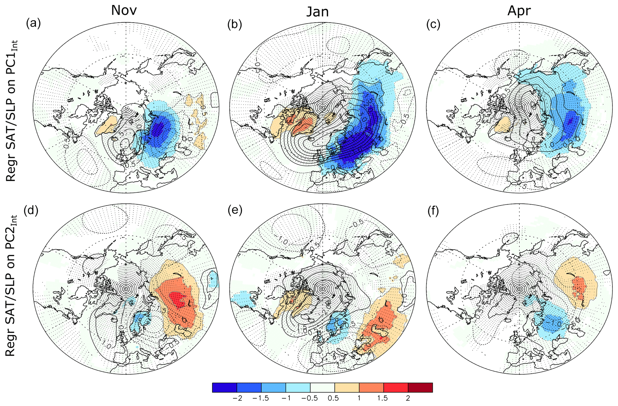
Figure 12Regression of the (color shading) 2 m air temperature (T2m, ∘C) and (black contour, contour interval 0.5 hPa) SLP (hPa) on (a–c) PC1Int and (c–e) PC2Int for (left, a, d, and g) November, (center, b, e, and h) January, and (right, c, f, and i) April. All regressions are calculated at no lag (lag 0 months) and only use the T2m and SLP anomalies associated with the internal atmosphere–land variability, after the removal of the corresponding multi-model mean. The regression shows the multi-model mean regression map, with dots indicating when the sign of SLP anomalies is consistent in at least seven models out of eight. The color shading is masked if the sign of T2m is not consistent in at least seven models out of eight.
The SLP and surface air temperature associated with the first mode are calculated by a regression onto the PC1Int of the snow cover in each model, which is then averaged similarly among all models. The snow EOF1Int in November, January, and April is always associated at no lag with an anticyclone located at the north or the northwest of the positive snow cover anomalies (Fig. 12a–c), as expected from cold air advection, which increases snow cover. However, the location and amplitude of the cold surface air temperature anomalies do not always match the snow cover anomalies. For instance, the cold anomalies are strongest in January with a widespread cooling extending from western Europe to far eastern Siberia, but the associated snow cover anomalies have the same amplitude in all 3 months and are only located over eastern Europe in January. In November, the anticyclone is centered over the Nordic seas (Fig. 12a), while it extends from the Nordic seas to northern Siberia in January (Fig. 12b). In April, the snow anomalies cover the southern edge of the snow cover domain, and the anticyclone is centered over the eastern Arctic (Fig. 12c). EOF2Int is associated with a trough over the Ural Mountains in November and April, while the NAO and the associated temperature anomalies over southern Siberia dominate in January.
The comparison between Fig. 10 for observations and Figs. 11 and 12 for models suggests that the models reproduce the main mode of the observed variability fairly well. In both cases, the NAO is the dominant mode of variability during January. In January, the analysis of the second EOF from detrended observations (not shown) also shows that it is associated with patterns similar to that found in models (Figs. 11e and 12e). During November and April, the observed dominant mode of variability is a blocking pattern with a trough over the Ural region. This pattern also occurs in the models, but with less variance, as it is reproduced by EOF2 rather than EOF1. However, there is an important spread among observations in November and April, and the analysis of observation is based on detrended time series that still include the contribution from interannual SST variability and short-term fluctuations in the external forcing.
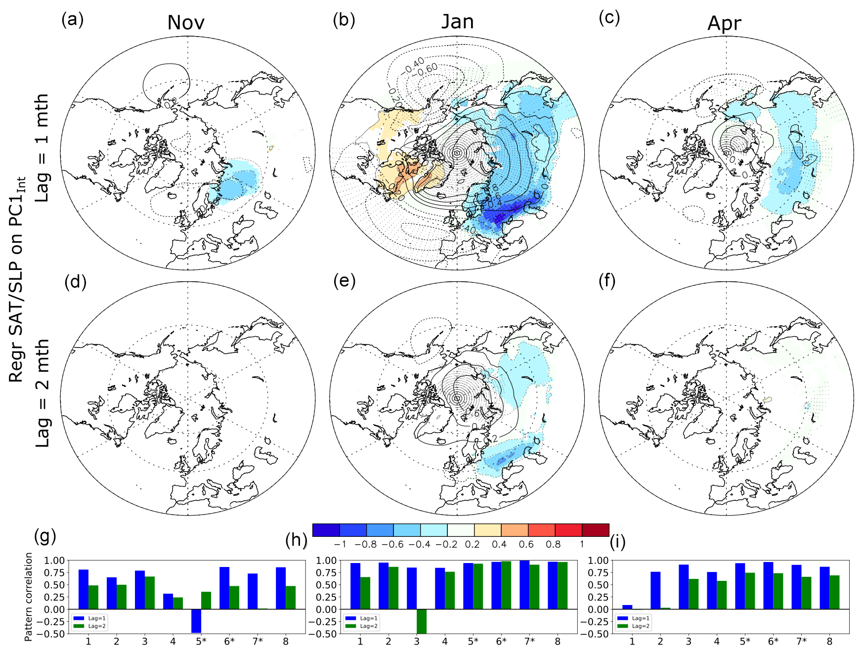
Figure 13Same as Fig. 12a–c, but at (a–c) lag 1 and (d–f) lag 2, when the atmosphere follows the (left, a, d) November, (center, b, e) January, and (right, c, f) April snow cover index by 1 month, as provided by PC1Int. The last row shows the spatial pattern correlation north of 20∘ N between the SLP regression obtained from each model and that of the model average. The blue (green) bar shows the results at lag 1 (2). The numbers on the x axis designate each model (see Table 1 for the corresponding model names). The star symbol indicates when 30 members are available for both ALL and NoSICvar for (g) November, (h) January, and (i) April.
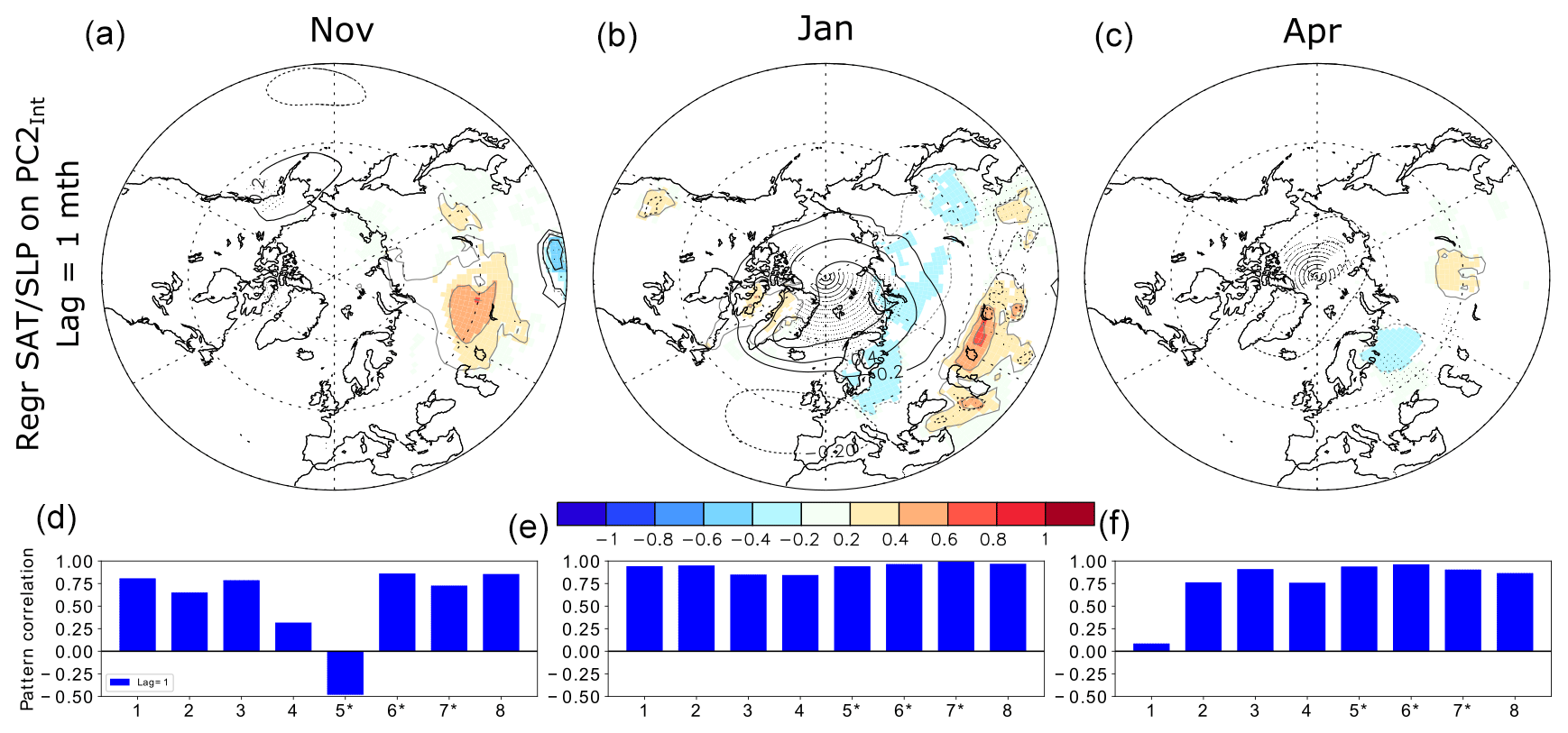
Figure 14Same as Fig. 12a–c, but using PC2Int instead of PC1Int at lag 1 month, when the atmosphere follows the (a) November, (b) January, and (c) April snow cover by 1 month. The last row shows the spatial pattern correlation north of 20∘ N between the SLP regression obtained from each model and that of the model average. The blue bar shows the results at lag 1. The numbers on the x axis designate each model (see Table 1 for the corresponding model names). The star symbol indicates when 30 members are available for both ALL and NoSICvar for (g) November, (h) January, and (i) April.
4.2 Climate influence of snow cover anomalies
Because of the limited intrinsic atmospheric persistence, the SLP and temperature lagging the snow cover by 1 month should reflect the snow cover influence in the absence of other concomitant forcings. It is illustrated for observations in Fig. 10c, g, and k and for models in Figs. 13 and 14. In observations, the November EOF1 is followed by negative SLP anomalies over the polar cap and some weak positive anomalies over western Europe and the Bering Sea. This SLP pattern shares some similarities with that found at no lag, but with a smaller amplitude. In January, the negative NAO anomalies associated in-phase with EOF1 are reduced by half but they persist the following month. In April, no clear SLP pattern emerges at a lag of 1 month. In all cases, the surface temperature is cold (warm) over positive (negative) snow cover anomalies, as expected, although their statistical significance is limited.
In models, no robust SLP or temperature anomalies follow the November snow cover EOF1Int with a lag of 1 or 2 months (Fig. 13a and d). On the other hand, the January EOF1Int (Fig. 13b) is followed by strong temperature and SLP anomalies at lag 1 (in February) with a strong anticyclonic anomaly over the polar cap extending toward central Eurasia, which is associated with cold continental air advection over northern Eurasia. The patterns are somewhat similar to those shown at lag 0 for January (Fig. 12b). Since they remain largely similar at lag 2 (Fig. 13e), albeit with smaller amplitude, this suggests that snow cover anomalies act as a positive feedback and amplify the AO 1 (in February) or 2 (in March) months later. However, it might also reflect an unusually large atmospheric persistence or the presence of a concomitant forcing. The May SLP and temperature anomalies lagging the EOF1Int in April by 1 month (Fig. 13c) are also similar to the unlagged patterns, albeit smaller, and the air temperature remains cold over the land surfaces covered with positive snow anomalies in April. However, the anomalies are negligible at lag 2 (Fig. 13f). The pattern lagging the snow cover by 1 month is robust among models in January (Fig. 13h), but the agreement decreases in April (Fig. 13i) and more so in November (Fig. 13g). For the pattern following the January EOF1Int by 2 months, the agreement among models is smaller than at lag 1, but it remains high in models with 30 members.
The temperature and SLP anomalies lagging the snow cover EOF2Int by 1 month (Fig. 14a–c) are smaller than for EOF1Int and they vanish at lag 2 (not shown). There are substantial temperature and SLP perturbations (Fig. 14b) 1 month after January EOF2Int, resembling a negative AO pattern, as was the case of the forcing pattern (Fig. 12e), but weaker. Its polar center is rather located over Svalbard, and it is less associated with an intensification of the Siberian anticyclone. Negative SLP anomalies are also found over East Asia. On the other hand, only small SLP and surface air temperature anomalies follow the November and April EOF2Int.
The comparison of Fig. 10 with Figs. 12 and 13 shows a different relationship in models and observations for snow cover in November and April. However, in January, more extended snow cover over Europe is followed in both models and observations by anticyclonic anomalies over Iceland and negative pressure anomalies over the midlatitude Atlantic Ocean, as well as cold air temperature advection toward Europe. As the same relationship is found when the January land snow leads the atmosphere by 2 months in models, this might indicate a large-scale atmospheric response to the snow cover anomalies. However, an anomalous persistence of atmospheric anomalies can also be caused by troposphere–stratosphere interactions, increasing the memory of the atmosphere. This hypothesis is investigated in the next section.
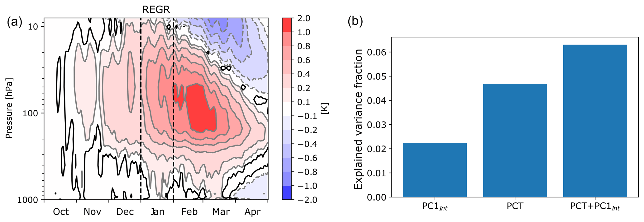
Figure 15(a) Regression of the daily air temperature anomalies over the polar cap (north of 60∘ N) (∘C) onto the first PC of the snow cover internal atmospheric variability, PC1Int, in January and in LMDZOR6. The black line indicates the local statistical significance at the 5 % level. The vertical dashed black line shows the days corresponding to January. (b) Explained variance fraction of the Arctic oscillation defined as the first EOF of the sea level pressure north of 20∘ N for a regression using PC1Int, PCT50, and both PCTInd and PCT50 as predictors. The explained variance fraction is significant at the 5 % level in the three cases.
4.3 Role of the stratosphere for the January snow cover variability
To understand the mechanism behind the statistical relationship between the January snow cover and the atmosphere, we focus on LMDZOR6 (model no. 5 in Figs. 11g–i, 12g–i, and 13g–i.), as daily outputs and three-dimensional atmospheric fields are available. LMDZOR6 reproduces the links between the January snow cover EOF1Int and the atmosphere 1 or 2 months later shown in Fig. 13, with nearly identical regression maps onto PC1Int (not shown). Figure 15 shows the lag regression of the daily polar cap temperature (north of 60∘ N) onto the PC1Int of the January snow cover. A significant lower-stratosphere warming is simulated from November to March. At 50 hPa, the temperature anomaly increases from 0.15 ∘C in November to 0.3 ∘C in December and 0.6 ∘C in January. The stratospheric warming and polar vortex weakening thus precede the January snow cover anomalies. However, the stratospheric temperature shows another maximum anomaly of 1.0 ∘C in February, suggesting that the snow cover has intensified the polar vortex weakening. The 50 hPa geopotential height anomalies associated with the snow cover show that the polar vortex weakening is widespread and affects the whole polar cap (Fig. S4).
The wave activity flux was calculated to investigate the propagation of the stationary waves (see Sect. 2.2). The regression of the wave activity flux on PC1Int shows an amplified upward component of the wave activity flux over eastern Eurasia and the western North Pacific (Fig. S5). This may weaken the polar vortex within 10 to 20 d. It is well established that such polar vortex weakening might then lead to a negative AO in the troposphere, with a lag of a few weeks (Baldwin and Dunkerton, 1999), and episodic downward propagations are indeed visible in Fig. 15 from mid-January to March. However, the role of the snow cover anomalies in this mechanism remains to be established.
To do so, we consider in the same model (e.g., LMDZOR6) an index of the stratospheric polar vortex, defined as the standardized January polar cap (north of 60∘ N) temperature anomalies at 50 hPa, hereinafter called PCT50. We also define a February AO index with the first PC of the SLP north of 20∘ N. The ensemble mean of that model is then removed from all time series. The correlation between PCT50 and PC1Int is weak (0.09) but significant. Both the January PCT50 and PC1Int are significantly correlated with the February AO, but the variance of the AO that is explained by PCT50 is larger than the one associated with the snow cover index, PC1Int (Fig. 15b). Both polar vortex and snow cover remain significantly related to the AO when using a multivariate regression (not shown). A similar analysis using composites confirms this result and shows that the relationships between both indices and the AO are mostly linear (Fig. S6). Therefore, the snow cover has a significant influence on the AO, but this influence is smaller than the one associated with the polar vortex.
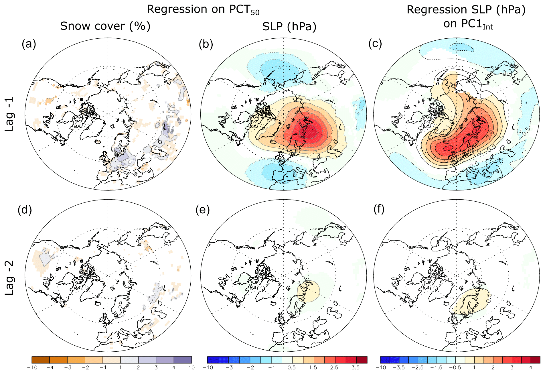
Figure 16Regression of the (a, d) snow cover (%) and sea level pressure (SLP; b, e) anomalies (hPa) onto the January polar cap (north of 60∘ N) 50 hPa temperature anomalies in LMDZOR6. (c, f) Regression of the sea level pressure (SLP) anomalies (hPa) onto the first PC of the snow cover internal atmospheric variability, PC1Int, in January and LMDZOR6. The lag indicated is negative and given in months, indicating that the polar cap 50 hPa geopotential height or the PC1Int lags. The color shading is masked if the local statistical significance is above 5 %.
Using regression onto PCT50, we found that the snow cover anomalies precede the stratospheric warming by 1 or 2 months (Fig. 16a and d), but not by more. The same regression using SLP (Fig. 16b and e) shows a dominant Ural blocking pattern in December, increasing the snow cover anomalies by easterly cold air advection and preceding the January polar vortex anomaly by 1 month. The Ural blocking is associated with negative SLP anomalies over western Europe and the Aleutians and thus projects onto the negative AO phase. Ural blocking can also amplify the stationary wave pattern and warm the stratosphere through intensified heat flux due to planetary waves (Martius et al., 2009; Peings, 2019). The regressions are weaker for lag −2, with only a small significant anticyclone east of Scandinavia. The Ural blocking pattern over northern Siberia is consistent with positive snow anomalies south of it. The regressions obtained using PCT50 (Fig. 16b and e) resemble the one obtained with PC1Int (Fig. 16c and f), even if the later anomalies are shifted toward the North Atlantic.
In summary, the snow cover and the polar vortex have a common driver, namely Ural tropospheric blocking. The snow cover and the polar vortex also have a similar influence on the AO 1 month later. Therefore, the lag relationship between January snow cover and the troposphere in February or March must be interpreted with caution, as causality cannot be firmly established. However, the polar vortex anomalies in Fig. 15 show a clear amplification in February, following the January snow cover anomalies. Although the snow cover influence is smaller than the one of the polar vortex, it remains significant when removing the concomitant effect of the polar vortex with a multivariate regression using snow cover and polar vortex indices. This suggests that snow cover anomalies act as a positive feedback for the AO variability, as they amplify the combined negative AO and Ural blocking pattern.
The land snow over the Northern Hemisphere is investigated in four observational datasets and two large multi-model ensembles of atmosphere-only experiments, one with prescribed SST, sea ice, and external forcing during the 1979–2014 period and the other in which sea ice variations are replaced by their climatology. Although models simulate different mean states for snow cover, the observations show an important spread as found by Mudryck et al. (2017), and both simulated trend and mean state are within the observational spread. In the multi-model ensemble mean, the trend is mainly driven by the external forcings and the associated SST warming. The sea ice loss only drives a small and insignificant fraction of snow cover trends. The sea ice loss only produces a decreasing snow cover trend located south and downstream of Scandinavia in January and April, as well as east of Scandinavia downstream of the Barents Sea in November. Cohen et al. (2014), among others, proposed that snow anomalies might amplify or damp the midlatitude atmospheric circulation response to sea ice loss, but in our experiments, the SIC has little influence in driving the snow cover. However, the lack of two-way coupling between atmosphere, sea ice, and the ocean in our experiments does not allow reproducing realistic links between snow and sea ice anomalies. Analogous analyses need to be conducted in AOGCMs to further investigate the links between SIC and snow cover.
The 1979–2014 investigated period shows a transition from a warm to a cold Interdecadal Pacific Oscillation (IPO) phase and from a cold to a warm Atlantic multidecadal variability (AMV) phase (Luo et al., 2022). Our analysis suggests that the IPO has a consistent influence among models on the North American snow cover through the PNA teleconnection pattern. The results for the Eurasian snow cover are ambiguous and cannot be specifically attributed to the SST anomalies or the external forcings. The investigation of simulations focusing on the role of external forcing, such as those realized in the RFMIP (Pincus et al., 2016) panel of CMIP6, would be necessary to distinguish between them. Sensitivity simulations using the observed changes in the AMV and IPO would also be helpful. In addition, including the period after 2014 would be important to understand the climate impacts of the observed reduction in spring snow cover (Mudryk et al., 2020). The simulations investigated here end in 2014 and cannot be used to fully understand this change. A similar multi-model investigation with simulations extended to the present day could be pursued in future works.
The snow cover variability due to internal atmosphere–land variability is analyzed in the large ensembles of simulation after removing the ensemble mean separately in each model. Lacking a better method, the internal variability is quantified in observations by removing the quadratic trend. We performed an EOF analysis of the Eurasian snow cover and used regression of atmospheric fields on the associated PCs to investigate the atmosphere–snow coupling. We found that the models reproduce the main atmospheric modes responsible for the forcing of the snow cover in observations well, with Ural blocking anomalies embedded with wave-like anomalies, leading to dipolar snow cover anomalies in early spring and early winter. In midwinter, the NAO has the dominant influence, increasing the snow cover over Europe and inducing a widespread Eurasian cooling for negative NAO phases. In both observations and models, we found no robust circulation pattern following November snow anomalies. This seems to contradict the results of Gastineau et al. (2017), wherein CMIP5 preindustrial control simulations were found to partly reproduce the observed influence of November Eurasian snow. This emphasizes the need to better explore the observational uncertainties using various datasets. However, sea ice concentration and SST anomalies are prescribed in our atmosphere-only simulations and cannot respond to the atmospheric forcing as in observations or coupled simulations, wherein snow cover, sea ice, and SST are driven by the atmosphere and provide concomitant forcings. Both models and observations show that January western Eurasia snow cover anomalies are linked to AO-like anomalies 1 month later. The relationship remains significant at a lag of 2 months in models. The outputs from one of the models reveal that the Ural blocking pattern acts as a common driver for the eastern Europe snow and the polar vortex anomalies. A stratospheric warming (cooling) event and a polar vortex weakening (strengthening) are therefore found to precede the snow cover and negative (positive) AO changes in January by 2 months. The stratospheric warming is found to explain a larger AO variance fraction than the snow cover. The lead–lag relationship between snow cover and the atmosphere might only stem from the internal atmospheric variability, as proposed by Blackport and Screen (2021) for the case of the sea ice–atmosphere interaction that shares a large similarity with the interaction discussed here. However, we note that polar vortex anomalies (Fig. 15) are reinforced in February, 1 month after snow cover anomalies, and are much weaker before January. Such asymmetry suggests that the snow cover intensifies the stratospheric warming and the resulting AO-like anomalies produced by downward propagation 1 month later. This mechanism is supported by the intensification of the upward-propagating planetary waves following a larger snow cover extent in January, as found by Lü et al. (2020). This suggests a two-way coupling between the snow cover and the internal atmospheric variability, with the snow cover anomalies amplifying the AO–Ural blocking anomalies that generated them, acting as a positive feedback in the land–troposphere–stratosphere system. This conclusion agrees with the results from subseasonal forecasts (Orsolini et al., 2016; Garfinkel et al., 2020), wherein the snow cover through troposphere–stratosphere interaction reinforces and prolongs the NAO.
Further investigating causality and the specific role of the snow cover would require sensitivity experiments controlling the land snow cover or the use of specific statistics to investigate the causation (San Liang, 2014; Runge et al., 2015).
This study is based on publicly available data for observations. The ERA5 (https://doi.org/10.24381/cds.f17050d7, Hersbach et al., 2019) and ERA5-Land (https://doi.org/10.24381/cds.68d2bb30, Muñoz-Sabater, 2019) data are available from the Copernicus Climate Change Service (C3S) Climate Data Store (CDS) at https://cds.climate.copernicus.eu (last access: 8 May 2020). The MERRA-2 data are available from the Goddard Earth Sciences data and Information Services Center at https://disc.gsfc.nasa.gov (last access: 28 October 2022; DOI: https://doi.org/10.5067/8S35XF81C28F, GMAO, 2015). The NOAA-CDR data are available from the National Centers for Environmental Information at https://www.ncei.noaa.gov (last access: 22 July 2019) (DOI: https://doi.org/10.7265/zzbm-2w05, Robinson and Estilow, 2021). The GlobSnow v3.0 data are available at https://doi.org/10.1594/PANGAEA.911944 (Luojus et al., 2020). The CanSISE data ara available from the National Snow and Ice Data Center at https://doi.org/10.5067/96ltniikJ7vd (Mudryk and Derksen, 2017). The climate model simulations are available upon request from the authors of this study. MATLAB code for data analysis and scripts used to generate the map (ferret and python) can be obtained upon request from the corresponding author. The Plumb wave activity flux is calculated using the code from Kazuaki Nishii (http://www.atmos.rcast.u-tokyo.ac.jp/nishii/programs/index.html, Nishii 2022).
The supplement related to this article is available online at: https://doi.org/10.5194/tc-17-2157-2023-supplement.
All authors contributed to the realization of the model simulations. GG conceived this study, performed the analysis, and wrote the first text version. All authors provided edits, comments, and inputs for writing the final text.
The contact author has declared that none of the authors has any competing interests.
Publisher's note: Copernicus Publications remains neutral with regard to jurisdictional claims in published maps and institutional affiliations.
The LOCEAN-IPSL group was granted access to the HPC resources of TGCC under allocations A5-017403 and A7-017403 made by GENCI.
The NorESM2-CAM6 simulations were performed on resources provided by UNINETT Sigma2 – the National Infrastructure for High-Performance Computing and Data Storage in Norway (nn2343k, NS9015K).
We have been supported by the Blue-Action project (European Union’s Horizon 2020 research and innovation program, no. 727852, http://www.blue-action.eu/index.php?id=3498, last access: 1 July 2022). Guillaume Gastineau and Claude Frankignoul were funded by the JPI Climate/JPI Oceans ROADMAP project (ANR-19-JPOC-003). Elisa Manzini and Daniela Matei received support from the German Federal Ministry of Education and Research through the JPI Climate/JPI Oceans NextG-Climate Science ROADMAP project (FKZ: 01LP2002A). Young-Oh Kwon, Claude Frankignoul, and Yu-Chiao Liang are supported by the US National Science Foundation, Office of Polar Programs (grant nos. OPP-1736738, OPP-2106190).
This paper was edited by Chris Derksen and reviewed by three anonymous referees.
Baldwin, M. P. and Dunkerton, T. J.: Propagation of the Arctic Oscillation from the stratosphere to the troposphere, J. Geophys. Res.-Atmos., 104, 30937–30946, https://doi.org/10.1029/1999JD900445, 1999.
Bentsen, M., Bethke, I., Debernard, J. B., Iversen, T., Kirkevåg, A., Seland, Ø., Drange, H., Roelandt, C., Seierstad, I. A., Hoose, C., and Kristjánsson, J. E.: The Norwegian Earth System Model, NorESM1-M – Part 1: Description and basic evaluation of the physical climate, Geosci. Model Dev., 6, 687–720, https://doi.org/10.5194/gmd-6-687-2013, 2013.
Blackport, R. and Screen, J. A.: Observed statistical connections overestimate the causal effects of arctic sea ice changes on midlatitude winter climate, J. Climate, 34, 3021–3038, 2021.
Brown, R. D. and Derksen, C.: Is Eurasian October snow cover extent increasing?, Environ. Res. Lett., 8, 024006, https://doi.org/10.1088/1748-9326/8/2/024006, 2013.
Brun, E., Six, D., Picard, G., Vionnet, V., Arnaud, L., Bazile, E., Boone, A., Bouchard, A., Genthon, C., Guidard, V., Moigne, P. L., Rabier, F., and Seity, Y.: Snow/atmosphere coupled simulation at Dome C, Antarctica, J. Glaciol., 57, 721–736, Cambridge Core, https://doi.org/10.3189/002214311797409794, 2011.
Cherchi, A., Fogli, P. G., Lovato, T., Peano, D., Iovino, D., Gualdi, S., Masina, S., Scoccimarro, E., Materia, S., Bellucci, A., and Navarra, A.: Global Mean Climate and Main Patterns of Variability in the CMCC-CM2 Coupled Model, J. Adv. Model. Earth Sy., 11, 185–209, https://doi.org/10.1029/2018MS001369, 2019.
Cohen, J. and Entekhabi, D.: Eurasian snow cover variability and Northern Hemisphere climate predictability, Geophys. Res. Lett., 26, 345–348, https://doi.org/10.1029/1998GL900321, 1999.
Cohen, J., Furtado, J. C., Jones, J., Barlow, M., Whittleston, D., and Entekhabi, D.: Linking Siberian Snow Cover to Precursors of Stratospheric Variability, J. Climate, 27, 5422–5432, https://doi.org/10.1175/JCLI-D-13-00779.1, 2014.
Dai, A. and Bloecker, C. E.: Impacts of internal variability on temperature and precipitation trends in large ensemble simulations by two climate models, Clim. Dynam., 52, 289–306, https://doi.org/10.1007/s00382-018-4132-4, 2019.
Derksen, C. and Brown, R.: Spring snow cover extent reductions in the 2008–2012 period exceeding climate model projections, Geophys. Res. Lett., 39, L19504, https://doi.org/10.1029/2012GL053387, 2012.
Déry, S. J. and Brown, R. D.: Recent Northern Hemisphere snow cover extent trends and implications for the snow-albedo feedback, Geophys. Res. Lett., 34, L22504, https://doi.org/10.1029/2007GL031474, 2007.
Deser, C., Tomas, R. A., and Peng, S.: The Transient Atmospheric Circulation Response to North Atlantic SST and Sea Ice Anomalies, J. Climate, 20, 4751–4767, https://doi.org/10.1175/JCLI4278.1, 2007.
Deser, C., Phillips, A., Bourdette, V., and Teng, H.: Uncertainty in climate change projections: The role of internal variability, Clim. Dynam., 38, 527–546, 2012.
Deser, C., Tomas, R. A., and Sun, L.: The Role of Ocean–Atmosphere Coupling in the Zonal-Mean Atmospheric Response to Arctic Sea Ice Loss, J. Climate, 28, 2168–2186, https://doi.org/10.1175/JCLI-D-14-00325.1, 2015.
Döscher, R., Acosta, M., Alessandri, A., Anthoni, P., Arsouze, T., Bergman, T., Bernardello, R., Boussetta, S., Caron, L.-P., Carver, G., Castrillo, M., Catalano, F., Cvijanovic, I., Davini, P., Dekker, E., Doblas-Reyes, F. J., Docquier, D., Echevarria, P., Fladrich, U., Fuentes-Franco, R., Gröger, M., v. Hardenberg, J., Hieronymus, J., Karami, M. P., Keskinen, J.-P., Koenigk, T., Makkonen, R., Massonnet, F., Ménégoz, M., Miller, P. A., Moreno-Chamarro, E., Nieradzik, L., van Noije, T., Nolan, P., O'Donnell, D., Ollinaho, P., van den Oord, G., Ortega, P., Prims, O. T., Ramos, A., Reerink, T., Rousset, C., Ruprich-Robert, Y., Le Sager, P., Schmith, T., Schrödner, R., Serva, F., Sicardi, V., Sloth Madsen, M., Smith, B., Tian, T., Tourigny, E., Uotila, P., Vancoppenolle, M., Wang, S., Wårlind, D., Willén, U., Wyser, K., Yang, S., Yepes-Arbós, X., and Zhang, Q.: The EC-Earth3 Earth system model for the Coupled Model Intercomparison Project 6, Geosci. Model Dev., 15, 2973–3020, https://doi.org/10.5194/gmd-15-2973-2022, 2022.
Eyring, V., Bony, S., Meehl, G. A., Senior, C. A., Stevens, B., Stouffer, R. J., and Taylor, K. E.: Overview of the Coupled Model Intercomparison Project Phase 6 (CMIP6) experimental design and organization, Geosci. Model Dev., 9, 1937–1958, https://doi.org/10.5194/gmd-9-1937-2016, 2016.
Feldstein, S. B.: The Timescale, Power Spectra, and Climate Noise Properties of Teleconnection Patterns, J. Climate, 13, 4430–4440, https://doi.org/10.1175/1520-0442(2000)013<4430:TTPSAC>2.0.CO;2, 2000.
Fletcher, C. G., Hardiman, S. C., Kushner, P. J., and Cohen, J.: The Dynamical Response to Snow Cover Perturbations in a Large Ensemble of Atmospheric GCM Integrations, J. Climate, 22, 1208–1222, https://doi.org/10.1175/2008JCLI2505.1, 2009.
Fox-Kemper, B., Hewitt, H. T., Xiao, C., Aðalgeirsdoìttir, G., Drijfhout, S. S., Edwards, T. L., Golledge, N. R., Hemer, M., Kopp, R. E., Krinner, G., Mix, A., Notz, D., Nowicki, S., Nurhati, I. S., Ruiz, L., Salle, J.-B., Slangen, A. B. A., and Yu, Y.: Ocean, Cryosphere and Sea Level Change, in: Climate Change 2021: The Physical Science Basis. Contribution of Working Group I to the Sixth Assessment Report of the Intergovernmental Panel on Climate Change, Cambridge University Press, Cambridge, UK and New York, NY, USA, 1211–1362, https://doi.org/10.1017/9781009157896.011, 2021.
García-Serrano, J., Frankignoul, C., Gastineau, G., and de la Cámara, A.: On the Predictability of the Winter Euro-Atlantic Climate: Lagged Influence of Autumn Arctic Sea Ice, J. Climate, 28, 5195–5216, https://doi.org/10.1175/JCLI-D-14-00472.1, 2015.
Garfinkel, C. I., Schwartz, C., White, I. P., and Rao, J.: Predictability of the early winter Arctic oscillation from autumn Eurasian snowcover in subseasonal forecast models, Clim. Dynam., 55, 961–974, https://doi.org/10.1007/s00382-020-05305-3, 2020.
Gastineau, G. and Frankignoul, C.: Influence of the North Atlantic SST Variability on the Atmospheric Circulation during the Twentieth Century, J. Climate, 28, 1396–1416, https://doi.org/10.1175/JCLI-D-14-00424.1, 2015.
Gastineau, G., García-Serrano, J., and Frankignoul, C.: The Influence of Autumnal Eurasian Snow Cover on Climate and Its Link with Arctic Sea Ice Cover, J. Climate, 30, 7599–7619, https://doi.org/10.1175/JCLI-D-16-0623.1, 2017.
Gastineau, G., Friedman, A. R., Khodri, M., and Vialard, J.: Global ocean heat content redistribution during the 1998–2012 Interdecadal Pacific Oscillation negative phase, Clim. Dynam., 53, 1187–1208, https://doi.org/10.1007/s00382-018-4387-9, 2019.
Ge, Y. and Gong, G.: North American snow depth and climate teleconnection patterns, J. Climate, 22, 217–233, https://doi.org/10.1175/2008JCLI2124.1, 2009.
Gelaro, R., McCarty, W., Suárez, M. J., Todling, R., Molod, A., Takacs, L., Randles, C. A., Darmenov, A., Bosilovich, M. G., Reichle, R., Wargan, K., Coy, L., Cullather, R., Draper, C., Akella, S., Buchard, V., Conaty, A., da Silva, A. M., Gu, W., Kim, G.-K., Koster, R., Lucchesi, R., Merkova, D., Nielsen, J. E., Partyka, G., Pawson, S., Putman, W., Rienecker, M., Schubert, S. D., Sienkiewicz, M., and Zhao, B.: The Modern-Era Retrospective Analysis for Research and Applications, Version 2 (MERRA-2), J. Climate, 30, 5419–5454, https://doi.org/10.1175/JCLI-D-16-0758.1, 2017.
Gettelman, A., Mills, M. J., Kinnison, D. E., Garcia, R. R., Smith, A. K., Marsh, D. R., Tilmes, S., Vitt, F., Bardeen, C. G., McInerny, J., Liu, H.-L., Solomon, S. C., Polvani, L. M., Emmons, L. K., Lamarque, J.-F., Richter, J. H., Glanville, A. S., Bacmeister, J. T., Phillips, A. S., Neale, R. B., Simpson, I. R., DuVivier, A. K., Hodzic, A., and Randel, W. J.: The Whole Atmosphere Community Climate Model Version 6 (WACCM6), J. Geophys. Res.-Atmos., 124, 12380–12403, https://doi.org/10.1029/2019JD030943, 2019.
Global Modeling and Assimilation Office (GMAO): MERRA-2 tavgM_2d_lnd_Nx: 2d, Monthly mean, Time-Averaged, Single-Level, Assimilation, Land Surface Diagnostics V5.12.4, Goddard Earth Sciences Data and Information Services Center (GES DISC), Greenbelt, MD, USA [data set], https://doi.org/10.5067/8S35XF81C28F (last access: 28 October 2022), 2015.
Gong, G., Entekhabi, D., and Cohen, J.: Modeled Northern Hemisphere Winter Climate Response to Realistic Siberian Snow Anomalies, J. Climate, 16, 3917–3931, https://doi.org/10.1175/1520-0442(2003)016<3917:MNHWCR>2.0.CO;2, 2003.
Gulev, S. K., Thorne, P. W., Ahn, J., Dentener, F. J., Domingues, C. M., Gerland, S., Gong, D., Kaufman, D. S., Nnamchi, H. C., Quaas, J., Rivera, J. A., Sathyendranath, S., Smith, S. L., Trewin, B., von Schuckmann, K., and Vose, R. S.: Changing State of the Climate System, in: Climate Change 2021: The Physical Science Basis. Contribution of Working Group I to the Sixth Assessment Report of the Intergovernmental Panel on Climate Change, edited by: Masson-Delmotte, V., Zhai, P., Pirani, A., Connors, S. L., Péan, C., Berger, S., Caud, N., Chen, Y., Goldfarb, L., Gomis, M. I., Huang, M., Leitzell, K., Lonnoy, E., Matthews, J. B. R., Maycock, T. K., Waterfield, T., Yelekçi, O., Yu, R., and Zhou, B., Cambridge University Press, Cambridge, UK and New York, NY, USA, 287–422, 2021.
Guo, H., Yang, Y., Zhang, W., Zhang, C., and Sun, H.: Attributing snow cover extent changes over the Northern Hemisphere for the past 65 years, Environmental Research Communications, 3, 061001, https://doi.org/10.1088/2515-7620/ac03c8, 2021.
Haarsma, R. J., Roberts, M. J., Vidale, P. L., Senior, C. A., Bellucci, A., Bao, Q., Chang, P., Corti, S., Fučkar, N. S., Guemas, V., von Hardenberg, J., Hazeleger, W., Kodama, C., Koenigk, T., Leung, L. R., Lu, J., Luo, J.-J., Mao, J., Mizielinski, M. S., Mizuta, R., Nobre, P., Satoh, M., Scoccimarro, E., Semmler, T., Small, J., and von Storch, J.-S.: High Resolution Model Intercomparison Project (HighResMIP v1.0) for CMIP6, Geosci. Model Dev., 9, 4185–4208, https://doi.org/10.5194/gmd-9-4185-2016, 2016.
Henderson, G. R., Peings, Y., Furtado, J. C., and Kushner, P. J.: Snow–atmosphere coupling in the Northern Hemisphere, Nat. Clim. Change, 8, 954–963, 2018.
Hersbach, H., Bell, B., Berrisford, P., Biavati, G., Horányi, A., Muñoz Sabater, J., Nicolas, J., Peubey, C., Radu, R., Rozum, I., Schepers, D., Simmons, A., Soci, C., Dee, D., and Thépaut, J.-N.: ERA5 monthly averaged data on single levels from 1959 to present, Copernicus Climate Change Service (C3S) Climate Data Store (CDS) [data set], https://doi.org/10.24381/cds.f17050d7 (last access: 8 May 2020), 2019.
Hersbach, H., Bell, B., Berrisford, P., Hirahara, S., Horányi, A., Muñoz-Sabater, J., Nicolas, J., Peubey, C., Radu, R., Schepers, D., Simmons, A., Soci, C., Abdalla, S., Abellan, X., Balsamo, G., Bechtold, P., Biavati, G., Bidlot, J., Bonavita, M., De Chiara, G., Dahlgren, P., Dee, D., Diamantakis, M., Dragani, R., Flemming, J., Forbes, R., Fuentes, M., Geer, A., Haimberger, L., Healy, S., Hogan, R. J., Hólm, E. Janisková, M., Keeley, S., Laloyaux, P., Lopez, P., Lupu, C., Radnoti, G., de Rosnay, P., Rozum, I., Vamborg, F., Villaume, S., Thépaut, J.-N.: The ERA5 global reanalysis, Q. J. Roy. Meteorol. Soc., 146, 1999–2049, https://doi.org/10.1002/qj.3803, 2020.
Honda, M., Inoue, J., and Yamane, S.: Influence of low Arctic sea-ice minima on anomalously cold Eurasian winters, Geophys. Res. Lett., 36, L08707, https://doi.org/10.1029/2008GL037079, 2009.
Hourdin, F., Rio, C., Grandpeix, J.-Y., Madeleine, J.-B., Cheruy, F., Rochetin, N., Jam, A., Musat, I., Idelkadi, A., Fairhead, L., Foujols, M.-A., Mellul, L., Traore, A.-K., Dufresne, J.-L., Boucher, O., Lefebvre, M.-P., Millour, E., Vignon, E., Jouhaud, J., Diallo, F. B., Lott, F., Gastineau, G., Caubel, A., Meurdesoif, Y., and Ghattas, J.: LMDZ6A: The Atmospheric Component of the IPSL Climate Model With Improved and Better Tuned Physics, J. Adv. Model. Earth Sy., 12, e2019MS001892. https://doi.org/10.1029/2019MS001892, 2020.
Hurrell, J. W., Hack, J. J., Shea, D., Caron, J. M., and Rosinski, J.: A New Sea Surface Temperature and Sea Ice Boundary Dataset for the Community Atmosphere Model, J. Climate, 21, 5145–5153, https://doi.org/10.1175/2008JCLI2292.1, 2008.
King, M. P., Hell, M., and Keenlyside, N.: Investigation of the atmospheric mechanisms related to the autumn sea ice and winter circulation link in the Northern Hemisphere, Clim. Dynam., 46, 1185–1195, https://doi.org/10.1007/s00382-015-2639-5, 2016.
Krinner, G., Derksen, C., Essery, R., Flanner, M., Hagemann, S., Clark, M., Hall, A., Rott, H., Brutel-Vuilmet, C., Kim, H., Ménard, C. B., Mudryk, L., Thackeray, C., Wang, L., Arduini, G., Balsamo, G., Bartlett, P., Boike, J., Boone, A., Chéruy, F., Colin, J., Cuntz, M., Dai, Y., Decharme, B., Derry, J., Ducharne, A., Dutra, E., Fang, X., Fierz, C., Ghattas, J., Gusev, Y., Haverd, V., Kontu, A., Lafaysse, M., Law, R., Lawrence, D., Li, W., Marke, T., Marks, D., Ménégoz, M., Nasonova, O., Nitta, T., Niwano, M., Pomeroy, J., Raleigh, M. S., Schaedler, G., Semenov, V., Smirnova, T. G., Stacke, T., Strasser, U., Svenson, S., Turkov, D., Wang, T., Wever, N., Yuan, H., Zhou, W., and Zhu, D.: ESM-SnowMIP: assessing snow models and quantifying snow-related climate feedbacks, Geosci. Model Dev., 11, 5027–5049, https://doi.org/10.5194/gmd-11-5027-2018, 2018.
Kug, J. S., Jeong, J. H., Jang, Y. S., Kim, B.-M., Folland, C. K., Min, S.-K., and Son, S.-W.: Two distinct influences of Arctic warming on cold winters over North America and East Asia, Nat. Geosci., 8, 759–762 https://doi.org/10.1038/ngeo2517, 2015.
Kushnir, Y., Robinson, W. A., Bladé, I., Hall, N. M. J., Peng, S., and Sutton, R.: Atmospheric GCM Response to Extratropical SST Anomalies: Synthesis and Evaluation, J. Climate, 15, 2233–2256, https://doi.org/10.1175/1520-0442(2002)015<2233:AGRTES>2.0.CO;2, 2002.
Lau, N.-C.: Interactions between Global SST Anomalies and the Midlatitude Atmospheric Circulation, B. Am. Meteorol. Soc., 78, 21–34, https://doi.org/10.1175/1520-0477(1997)078<0021:IBGSAA>2.0.CO;2, 1997.
Liang, Y.-C., Kwon, Y.-O., Frankignoul, C., Danabasoglu, G., Yeager, S., Cherchi, A., Gao, Y., Gastineau, G., Ghosh, R., Matei, D., Mecking, J. V., Peano, D., Suo, L., and Tian, T.: Quantification of the Arctic Sea Ice-Driven Atmospheric Circulation Variability in Coordinated Large Ensemble Simulations, Geophys. Res. Lett., 47, e2019GL085397, https://doi.org/10.1029/2019GL085397, 2020.
Liang, Y.-C., Frankignoul, C., Kwon, Y.-O., Gastineau, G., Manzini, E., Danabasoglu, G., Suo, L., Yeager, S., Gao, Y., Attema, J. J., Cherchi, A., Ghosh, R., Matei, D., Mecking, J. V., Tian, T., and Zhang, Y.: Impacts of Arctic Sea Ice on Cold Season Atmospheric Variability and Trends Estimated from Observations and a Multimodel Large Ensemble, J. Climate, 34, 8419–8443, https://doi.org/10.1175/JCLI-D-20-0578.1, 2021.
López-Parages, J., Rodríguez-Fonseca, B., Dommenget, D., and Frauen, C.: ENSO influence on the North Atlantic European climate: A non-linear and non-stationary approach, Clim. Dynam., 47, 2071–2084, https://doi.org/10.1007/s00382-015-2951-0, 2016.
Lü, Z., Li, F., Orsolini, Y. J., Gao, Y., and He, S.: Understanding of European Cold Extremes, Sudden Stratospheric Warming, and Siberian Snow Accumulation in the Winter of 2017/18, J. Climate, 33, 527–545, https://doi.org/10.1175/JCLI-D-18-0861.1, 2020.
Luo, B., Luo, D., Dai, A., Simmonds, I., and Wu, L.: The modulation of Interdecadal Pacific Oscillation and Atlantic Multidecadal Oscillation on winter Eurasian cold anomaly via the Ural blocking change, Clim. Dynam., 59, 127–150, https://doi.org/10.1007/s00382-021-06119-7, 2022.
Luojus, K., Pulliainen, J., Takala, M., Lemmetyinen, J., and Moisander, M.: GlobSnow v3.0 snow water equivalent (SWE), PANGAEA, [data set] https://doi.org/10.1594/PANGAEA.911944 (last access: 15 July 2020), 2020.
Martius, O., Polvani, L. M., and Davies, H. C.: Blocking precursors to stratospheric sudden warming events, Geophys. Res. Lett., 36, L14806, https://doi.org/10.1029/2009GL038776, 2009.
Mathieu, P.-P., Sutton, R. T., Dong, B., and Collins, M.: Predictability of Winter Climate over the North Atlantic European Region during ENSO Events, J. Climate, 17, 1953–1974, https://doi.org/10.1175/1520-0442(2004)017<1953:POWCOT>2.0.CO;2, 2004.
Mori, M., Watanabe, M., Shiogama, H., Inoue, J., and Kimoto, M.: Robust Arctic sea-ice influence on the frequent Eurasian cold winters in past decades, Nat. Geosci., 7, 869–873, https://doi.org/10.1038/ngeo2277, 2014.
Mudryk, L. R. and Derksen, C.: CanSISE Observation-Based Ensemble of Northern Hemisphere Terrestrial Snow Water Equivalent, Version 2, [Daily B5 SWE], NASA National Snow and Ice Data Center Distributed Active Archive Center, Boulder, Colorado, USA [data set], https://doi.org/10.5067/96ltniikJ7vd (last access: 16 August 2019), 2017.
Mudryk, L. R., Derksen, C., Kushner, P., and Brown, R.: Characterization of Northern Hemisphere Snow Water Equivalent Datasets, 1981–2010, J. Climate, 28, 8037–8051, https://doi.org/10.1175/JCLI-D-15-0229.1, 2015.
Mudryk, L. R., Kushner, P. J., Derksen, C., and Thackeray, C.: Snow cover response to temperature in observational and climate model ensembles, Geophys. Res. Lett., 44, 919–926, https://doi.org/10.1002/2016GL071789, 2017.
Mudryk, L., Santolaria-Otín, M., Krinner, G., Ménégoz, M., Derksen, C., Brutel-Vuilmet, C., Brady, M., and Essery, R.: Historical Northern Hemisphere snow cover trends and projected changes in the CMIP6 multi-model ensemble, The Cryosphere, 14, 2495–2514, https://doi.org/10.5194/tc-14-2495-2020, 2020.
Müller, W. A., Jungclaus, J. H., Mauritsen, T., Baehr, J., Bittner, M., Budich, R., Bunzel, F., Esch, M., Ghosh, R., Haak, H., Ilyina, T., Kleine, T., Kornblueh, L., Li, H., Modali, K., Notz, D., Pohlmann, H., Roeckner, E., Stemmler, I., Tian, F., and Marotzke, J.: A Higher-resolution Version of the Max Planck Institute Earth System Model (MPI-ESM1.2-HR), J. Adv. Model. Earth Sy., 10, 1383–1413, https://doi.org/10.1029/2017MS001217, 2018.
Muñoz-Sabater, J.: ERA5-Land monthly averaged data from 1981 to present, Copernicus Climate Change Service (C3S) Climate Data Store (CDS) [data set], https://doi.org/10.24381/cds.68d2bb30 (last access: 4 April 2020), 2019.
Muñoz-Sabater, J., Dutra, E., Agustí-Panareda, A., Albergel, C., Arduini, G., Balsamo, G., Boussetta, S., Choulga, M., Harrigan, S., Hersbach, H., Martens, B., Miralles, D. G., Piles, M., Rodríguez-Fernández, N. J., Zsoter, E., Buontempo, C., and Thépaut, J.-N.: ERA5-Land: a state-of-the-art global reanalysis dataset for land applications, Earth Syst. Sci. Data, 13, 4349–4383, https://doi.org/10.5194/essd-13-4349-2021, 2021.
Nakamura, T., Yamazaki, K., Iwamoto, K., Honda, M., Miyoshi, Y., Ogawa, Y., and Ukita, J.: A negative phase shift of the winter AO/NAO due to the recent Arctic sea-ice reduction in late autumn, J. Geophys. Res.-Atmos., 120, 3209–3227, https://doi.org/10.1002/2014JD022848, 2015.
Newman, M., Alexander, M. A., Ault, T. R., Cobb, K. M., Deser, C., Di Lorenzo, E., Mantua, N. J., Miller, A. J., Minobe, S., Nakamura, H., Vimont, D. J., Phillips, A. S., Scott, J. D., and Smith, C. A.: The Pacific decadal oscillation, revisited, J. Climate, 29, 4399–4427, 2016.
Nishii, K.: Programs for calculationg wave-activity flux derived by Takaya and Nakamura (2001, JAS: TN01) or by Plumb (1985, JAS) [code], http://www.atmos.rcast.u-tokyo.ac.jp/nishii/programs/index.html (last access: 20 June 2022), 2022.
Ogawa, F., Keenlyside, N., Gao, Y., Koenigk, T., Yang, S., Suo, L., Wang, T., Gastineau, G., Nakamura, T., Cheung, H. N., Omrani, N.-E., Ukita, J., and Semenov, V.: Evaluating impacts of recent Arctic sea ice loss on the Northern Hemisphere winter climate change, Geophys. Res. Lett., 45, 3255–3263, 2018.
Orsolini, Y. J., Senan, R., Balsamo, G., Doblas-Reyes, F. J., Vitart, F., Weisheimer, A., Carrasco, A., and Benestad, R. E.: Impact of snow initialization on sub-seasonal forecasts, Clim. Dynam., 41, 1969–1982, https://doi.org/10.1007/s00382-013-1782-0, 2013.
Orsolini, Y. J., Senan, R., Vitart, F., Balsamo, G., Weisheimer, A., and Doblas-Reyes, F. J.: Influence of the Eurasian snow on the negative North Atlantic Oscillation in subseasonal forecasts of the cold winter 2009/2010, Clim. Dynam., 47, 1325–1334, https://doi.org/10.1007/s00382-015-2903-8, 2016.
Paik, S. and Min, S. K.: Quantifying the Anthropogenic Greenhouse Gas Contribution to the Observed Spring Snow-Cover Decline Using the CMIP6 Multimodel Ensemble, J. Climate, 33, 9261–9269, 2020.
Peings, Y.: Ural blocking as a driver of early-winter stratospheric warmings, Geophys. Res. Lett., 46, 5460–5468, https://doi.org/10.1029/2019GL082097, 2019.
Peings, Y. and Magnusdottir, G.: Response of the wintertime Northern Hemisphere atmospheric circulation to current and projected Arctic sea ice decline: A numerical study with CAM5, J. Climate, 27, 244–264, 2014.
Perlwitz, J. and Graf, H.-F.: The Statistical Connection between Tropospheric and Stratospheric Circulation of the Northern Hemisphere in Winter, J. Climate, 8, 2281–2295, https://doi.org/10.1175/1520-0442(1995)008<2281:TSCBTA>2.0.CO;2, 1995.
Pincus, R., Forster, P. M., and Stevens, B.: The Radiative Forcing Model Intercomparison Project (RFMIP): experimental protocol for CMIP6, Geosci. Model Dev., 9, 3447–3460, https://doi.org/10.5194/gmd-9-3447-2016, 2016.
Plumb, R. A.: On the Three-Dimensional Propagation of Stationary Waves, J. Atmos. Sci., 42, 217–229, https://doi.org/10.1175/1520-0469(1985)042<0217:OTTDPO>2.0.CO;2, 1985.
Pulliainen, J., Aurela, M., Laurila, T., Aalto, T., Takala, M., Salminen, M., Kulmala, M., Barr, A., Heimann, M., Lindroth, A., Laaksonen, A., Derksen, C., Mäkelä, A., Markanen, T., Lemmetyinen, J., Susiluoto, J., Dengel, S., Mammarella, I., Tuovinen, J.-P., and Vesala, T.: Early snowmelt significantly enhances boreal springtime carbon uptake, P. Natl. Acad. Sci. USA, 114, 11081–11086, 2017.
Pulliainen, J., Luojus, K., Derksen, C., Mudryk, L., Lemmetyinen, J., Salminen, M., Ikonen, J., Takala, M., Cohen, J., Smolander, T., and Norberg, J.: Patterns and trends of Northern Hemisphere snow mass from 1980 to 2018, Nature, 581, 294–298, https://doi.org/10.1038/s41586-020-2258-0, 2020.
Robinson, D. A. and Estilow, T. W.: Rutgers Northern Hemisphere 24 km Weekly Snow Cover Extent, September 1980 Onward, Version 1, NSIDC: National Snow and Ice Data Center, Boulder, Colorado, USA [data set], https://doi.org/10.7265/zzbm-2w05 (last access: 22 July 2019), 2021.
Rodell, M., Houser, P. R., Jambor, U., Gottschalck, J., Mitchell, K., Meng, C.-J., Arsenault, K., Cosgrove, B., Radakovich, J., Bosilovich, M., Entin, J. K., Walker, J. P., Lohmann, D., and Toll, D.: The Global Land Data Assimilation System, B. Am. Meteorol. Soc., 85, 381–394, https://doi.org/10.1175/BAMS-85-3-381, 2004.
Runge, J., Petoukhov, V., Donges, J. F., Hlinka, J., Jajcay, N., Vejmelka, M., Hartman, D., Marwan, N., Paluš, N., and Kurths, J.: Identifying causal gateways and mediators in complex spatio-temporal systems, Nat. Commun., 6, 1–10, 2015.
Saito, K. and Cohen, J.: The potential role of snow cover in forcing interannual variability of the major Northern Hemisphere mode, Geophys. Res. Lett., 30, 1302, https://doi.org/10.1029/2002GL016341, 2003.
San Liang, X.: Unraveling the cause-effect relation between time series, Phys. Rev. E, 90, 052150, https://doi.org/10.1103/PhysRevE.90.052150, 2014.
Scaife, A. A., Arribas, A., Blockley, E., Brookshaw, A., Clark, R. T., Dunstone, N., Eade, R., Fereday, D., Folland, C. K., Gordon, M., Hermanson, L., Knight, J. R., Lea, D. J., MacLachlan, C., Maidens, A., Martin, M., Peterson, A. K., Smith, D., Vellinga, M., Wallace, E., Waters, J., Williams, A.: Skillful long-range prediction of European and North American winters, Geophys. Res. Lett., 41, 2514–2519, https://doi.org/10.1002/2014GL059637, 2014.
Seland, Ø., Bentsen, M., Olivié, D., Toniazzo, T., Gjermundsen, A., Graff, L. S., Debernard, J. B., Gupta, A. K., He, Y.-C., Kirkevåg, A., Schwinger, J., Tjiputra, J., Aas, K. S., Bethke, I., Fan, Y., Griesfeller, J., Grini, A., Guo, C., Ilicak, M., Karset, I. H. H., Landgren, O., Liakka, J., Moseid, K. O., Nummelin, A., Spensberger, C., Tang, H., Zhang, Z., Heinze, C., Iversen, T., and Schulz, M.: Overview of the Norwegian Earth System Model (NorESM2) and key climate response of CMIP6 DECK, historical, and scenario simulations, Geosci. Model Dev., 13, 6165–6200, https://doi.org/10.5194/gmd-13-6165-2020, 2020.
Simon, A., Frankignoul, C., Gastineau, G., and Kwon, Y. O.: An observational estimate of the direct response of the cold-season atmospheric circulation to the Arctic Sea Ice Loss, J. Climate, 33, 3863–3882, 2020.
Smith, D. M., Eade, R., Andrews, M. B., Ayres, H., Clark, A., Chripko, S., Deser, C., Dunstone, N. J., Garcia-Serrano, J., Gastineau, G., Graff, L. S., Hardiman, S. C., He, B., Hermanson, L., Jung, T., Knight, J., Levine, X., Magnusdottir, G., Manzini, E., Matei, D., Mori, M., Msadek, R., Ortega, P., Peings, Y., Scaiffe, A. A., Screen, J. A., Seabrook, M., Semmler, T., Sigmond, M., Streffing, J., Sun, L., and Walsh, A.: Robust but weak winter atmospheric circulation response to future Arctic sea ice loss, Nat. Commun., 13, 1–15, 2022.
Stevens, B., Giorgetta, M., Esch, M., Mauritsen, T., Crueger, T., Rast, S., Salzmann, M., Schmidt, H., Bader, J., Block, K., Brokopf, R., Fast, I., Kinne, S., Kornblueh, L., Lohmann, U., Pincus, R., Reichler, T., and Roeckner, E.: Atmospheric component of the MPI-M Earth System Model : ECHAM6, J. Adv. Model. Earth Sy., 5, 146–172, https://doi.org/10.1002/jame.20015, 2013.
Storch, H. and Zwiers, F.: Statistical Analysis in Climate Research, Cambridge University Press, Cambridge, ISBN 9780511612336, https://doi.org/10.1017/CBO9780511612336, 1999.
Sturm, M., Taras, B., Liston, G. E., Derksen, C., Jonas, T., and Lea, J.: Estimating Snow Water Equivalent Using Snow Depth Data and Climate Classes, J. Hydrometeorol., 11, 1380–1394, https://doi.org/10.1175/2010JHM1202.1, 2010.
Wallace, J. M. and Gutzler, D. S.: Teleconnections in the Geopotential Height Field during the Northern Hemisphere Winter, Mon. Weather Rev., 109, 784–812, https://doi.org/10.1175/1520-0493(1981)109<0784:TITGHF>2.0.CO;2, 1981.
Walters, D., Baran, A. J., Boutle, I., Brooks, M., Earnshaw, P., Edwards, J., Furtado, K., Hill, P., Lock, A., Manners, J., Morcrette, C., Mulcahy, J., Sanchez, C., Smith, C., Stratton, R., Tennant, W., Tomassini, L., Van Weverberg, K., Vosper, S., Willett, M., Browse, J., Bushell, A., Carslaw, K., Dalvi, M., Essery, R., Gedney, N., Hardiman, S., Johnson, B., Johnson, C., Jones, A., Jones, C., Mann, G., Milton, S., Rumbold, H., Sellar, A., Ujiie, M., Whitall, M., Williams, K., and Zerroukat, M.: The Met Office Unified Model Global Atmosphere 7.0/7.1 and JULES Global Land 7.0 configurations, Geosci. Model Dev., 12, 1909–1963, https://doi.org/10.5194/gmd-12-1909-2019, 2019.
Zhang, H., Zhang, M., and Zeng, Q.: Sensitivity of Simulated Climate to Two Atmospheric Models : Interpretation of Differences between Dry Models and Moist Models, Mon. Weather Rev., 141, 1558–1576, https://doi.org/10.1175/MWR-D-11-00367.1, 2013.
Zhong, X., Zhang, T., Kang, S., and Wang, J.: Snow depth trends from CMIP6 models conflict with observational evidence, J. Climate, 35, 1293–1307, https://doi.org/10.1175/JCLI-D-21-0177.1, 2022.
- Abstract
- Introduction
- Data and methods
- Simulated Northern Hemisphere snow cover and depth
- Internal variability and climate impacts of snow cover anomalies
- Discussion and conclusion
- Code and data availability
- Author contributions
- Competing interests
- Disclaimer
- Acknowledgements
- Financial support
- Review statement
- References
- Supplement