the Creative Commons Attribution 4.0 License.
the Creative Commons Attribution 4.0 License.
 | 25 May 2023
Simulating the Laurentide Ice Sheet of the Last Glacial Maximum
Jorge Alvarez-Solas
Javier Blasco
Marisa Montoya
Alexander Robinson
In the last decades, great effort has been made to reconstruct the Laurentide Ice Sheet (LIS) during the Last Glacial Maximum (LGM; ca. 21 000 years before present, 21 kyr ago). Uncertainties underlying its modelling have led to notable differences in fundamental features such as its maximum elevation, extent and total volume. As a result, the uncertainty in ice dynamics and thus in ice extent, volume and ice stream stability remains large. We herein use a higher-order three-dimensional ice sheet model to simulate the LIS under LGM boundary conditions for a number of basal friction formulations of varying complexity. Their consequences for the Laurentide ice streams, configuration, extent and volume are explicitly quantified. Total volume and ice extent generally reach a constant equilibrium value that falls close to prior LIS reconstructions. Simulations exhibit high sensitivity to the dependency of the basal shear stress on the sliding velocity. In particular, a regularised Coulomb friction formulation appears to be the best choice in terms of ice volume and ice stream realism. Pronounced differences are found when the basal friction stress is thermomechanically coupled: the base remains colder, and the LIS volume is lower than in the purely mechanical friction scenario counterpart. Thermomechanical coupling is fundamental for producing rapid ice streaming, yet it leads to a similar ice distribution overall.
- Article
(6148 KB) - Full-text XML
- BibTeX
- EndNote


The Laurentide Ice Sheet (LIS) was the largest of the former Northern Hemisphere ice sheets during the Last Glacial Maximum (LGM; ca. 21 000 years before present, 21 kyr ago). The LIS may have advanced to its maximum extent as early as 29–27 kyr ago, well before the LGM, and remained near that limit until 17 kyr ago (Dyke et al., 2002; Tarasov et al., 2012). Consequently, the LIS was the main contributor to sea-level change during the last glacial period, with an estimated sea-level equivalent (SLE) of about 70 m (28×106 km3) with respect to present (Peltier, 2004; Tarasov et al., 2012).
Great effort has been made to reconstruct the LIS at the LGM throughout the last 5 decades (note that we use the term Laurentide Ice Sheet in the broadest sense and include the Cordilleran and Innuitian ice sheets). Several approaches are found in the literature. The first numerical methods relied on simplified ice physics, a prescribed ice accumulation rate and ice surface temperature, and the assumption that the ice sheet was in a steady state (e.g. Paterson, 1972; Sugden, 1977; Hughes et al., 1980). This assumption was later relaxed by Mahaffy (1976) and Jenssen (1977), though the model was not applied to the late glacial history of the LIS. A completely independent approach was taken by Clark (1980) based on an inversion study of sea-level data where none of the previous assumptions are applied. Strictly speaking, the inversion solely shared the ice extent with prior studies, which is, in general, well known. This further allowed for independent tests of the reliability of such assumptions by comparison among ice sheets.
Reconstructions of the size and distribution of the LIS based on forward ice sheet modelling at the LGM have long dealt with the implications of a heterogeneous bedrock geology on the ice sheet flow dynamics (e.g. Calov et al., 2002; Tarasov and Peltier, 2004). The central core of the LIS rests on a hard bedrock of the Canadian shield, whereas nearly the entire Hudson Bay and Hudson Strait consist of Paleozoic carbonates easily eroded into a soft, slippery base. In view of this configuration, two approaches were classically taken. First, a simplification of the bedrock complexity was made by ignoring this deformable bed, thus resulting in a single-domed reconstruction centred over Hudson Bay (Denton and Hughes, 1981). The second approach considered lubricated basal conditions by reducing the maximum basal shear stress. Unlike the previous results, the reconstructions presented a multi-domed ice sheet with a thinner ice sheet and a less steep slope over Hudson Bay (Boulton et al., 1985; Fisher et al., 1985). This multi-domed configuration is also found in recent reconstructions (Tarasov et al., 2012; Gowan et al., 2021).
As a result of fundamental uncertainties underlying ice sheet modelling of the LIS, its maximum elevation, extent and total volume differ largely among studies (Stokes, 2017). In particular, the total volume carries the greatest uncertainty. Originally, Ramsay (1931) estimated a total LIS volume of 45.45×10⁶ km3, with a 15.75×10⁶ km2 extent and a maximum elevation of 2.9 km (here, and subsequently, above present sea level). More than 3 decades later, Paterson (1972) provided a significantly lower volume estimation of 26.5×10⁶ km3 with 11.6×10⁶ km2 ice-covered area and 2.7 km maximum ice thickness. The lowest overall volume estimate was given by Peltier (1994) (ICE-4G) with 19.0×10⁶ km3, whereas more recent studies yield 28×106 km3 (Tarasov et al., 2012) and 35×106 km3 (including the Cordilleran Ice Sheet; Gregoire et al., 2012).
Already noted by Clark (1980), the LIS may have never attained a steady state, and it was possibly a rather dynamic system with rapid variations in its southern margin as well as a variable Hudson Bay ice thickness. MacAyeal (1993a) later proposed a mechanism by which Hudson Bay would periodically switch from a quiescent to a surging state (controlling the flux of ice through the Hudson Strait ice stream) and further tested his theoretical prediction with a simple model (MacAyeal, 1993b). In fact, the LIS mass loss is intimately related to a variable Hudson Bay ice thickness through rapidly flowing ice streams that account for most of the ice sheet discharge (Stokes and Tarasov, 2010). Nevertheless, the representation of these ice streams into numerical ice sheet models remains challenging. As a result, we lack a deeper comprehension of the role of ice streams, which leads to larger model output uncertainties.
The reconstruction of paleo-ice streams is typically based on two methods. The first one rests on the assumption that the subglacial imprint of streaming and non-streaming areas is distinct (e.g. Kleman et al., 1997; Stokes and Clark, 1999) and consists of gathering enough evidence from landforms and sediments so as to reproduce their dynamics (e.g. Winsborrow et al., 2004; Ottesen et al., 2005). The second one is, again, based on forward ice sheet modelling using numerical models capable of simulating ice streaming (e.g. Boulton and Hagdorn, 2006). This ability is usually provided by thermomechanical feedbacks in topographic troughs and parametrisations of ice–bed coupling strength over soft sediments (Marshall et al., 1996).
Despite the comprehensive work carried out in the last decades, none of these studies addressed the repercussions of different basal friction formulations when simulating the LIS during the LGM nor their explicit implications in ice extent, volume and ice stream representation. In fact, recent studies have shown significant consequences of this uncertainty for the Antarctic Ice Sheet (e.g. Blasco et al., 2021). We herein consider three scenarios of varying dynamic complexity and their consequences for the Laurentide ice streams, configuration, extent and volume among other things. In Sect. 2, the main features of our model are described; results are shown in Sect. 3; a discussion is given in Sect. 4; and the conclusions of this work are presented in Sect. 5.
Numerical experiments are conducted with the higher-order three-dimensional ice sheet model Yelmo (Robinson et al., 2020, 2022). Here, its domain covers the entire LIS topography with a 16 km horizontal resolution. We set 21 unevenly spaced vertical levels in sigma coordinates, with higher resolution at the base of the ice sheet. Yelmo uses a higher-order stress approximation known as depth-integrated viscosity approximation (DIVA) to compute the horizontal velocity (Goldberg, 2011; Lipscomb et al., 2019). DIVA replaces the horizontal velocity gradients with their vertical averages in the effective strain rate, thus leading to a set of equations similar in accuracy to the Blatter–Pattyn approximation (Blatter, 1995; Pattyn, 2003). The internal ice temperature is determined by the advection–diffusion equation. Anisotropy of the ice is not explicitly modelled, so an enhancement factor accounts for crystal orientation on the strain rate (Hooke, 2005; Ma et al., 2010; Pollard and DeConto, 2012; Maris et al., 2014; Albrecht et al., 2020). For simplicity here, the enhancement factor of grounded ice is prescribed to be 1.0, whereas floating ice requires a slightly lower value of 0.7 (e.g. Ma et al., 2010).
The total mass balance in Yelmo is governed by three terms: surface mass balance, calving and basal melting. Calving occurs when the ice front thickness decreases below an imposed threshold (200 m in this study), and the upstream ice flux is not large enough to advect the necessary ice to maintain such thickness (Peyaud et al., 2007). Importantly, basal melting of floating ice is a boundary condition, whereas it is calculated internally for grounded ice.
2.1 Ice temperature
Yelmo accounts for a classical energy balance governed by an advection–diffusion equation:
where k and c are the ice thermal conductivity and specific heat capacity respectively. The ice temperature evolution is thus determined by vertical diffusion, horizontal and vertical advection, and internal strain-heat dissipation due to shearing Φ:
where is the effective strain rate, and ν is the ice viscosity.
For grounded ice, when the ice temperature is below the pressure melting point, the prescribed vertical gradient at the base is , where Qr is the heat flow at the bedrock surface. The geothermal heat flow Qgeo is then imposed as a boundary condition at 2 km below the bedrock surface. In other words, heat is diffused vertically within the first 2 km of the bedrock, which allows the model to account for the thermal inertia within the bedrock itself (Ritz, 1987).
If the basal ice temperature reaches the pressure melting point, the temperature is then set to the pressure melting point, and the basal mass balance bg is diagnosed following Alley (2011):
where the sign indicates melting when bg<0. Li is the latent heat of fusion for ice, Qb is the basal heat production due to sliding friction, and is the ice temperature vertical gradient at the base.
2.2 Till hydrology
The subglacial water-flow model assumes a thin film of water. Yelmo then considers a local evolution equation for the basal water content Hw without horizontal advection (considering a hydraulic diffusion coefficient m2 s−1; e.g. Tulaczyk et al., 2000a). In this case, the non-local term of the time-dependent diffusion equation is assumed to be negligible, yielding the following approximation:
Here, ρw is the water density; is basal mass balance defined in Eq. (3), given by the sum of the frictional heating at the ice–bed interface and the gradients in heat flow at the base of the ice column and at the bedrock surface (Eq. 4); and dr is the till drainage rate, set to m yr−1 (Bueler and van Pelt, 2015) in the default case, which means that its value is generally small compared to . Negative values of are allowed, implying refreezing. The water layer thickness is bounded between zero and a maximum value of Hw,max (Bueler and Brown, 2009; Bueler and van Pelt, 2015):
By default, Hw,max is set to a constant value of 2 m for simplicity (as in Bueler and van Pelt, 2015).
2.3 Friction
Basal shear stress can be generally expressed as a function of the sliding velocity ub and the effective pressure N, i.e. ). The physical properties of the material over which the ice may potentially slide can correspond to either a hard bedrock flow (e.g. Weertman, 1957) or a Coulomb–plastic rheology. In addition, the influence of the sliding velocity on τb is often represented by a power friction law, although a regularisation term u0 accounting for local properties of the bed has been shown to outperform such a power law in several contexts (Joughin et al., 2019; Zoet and Iverson, 2020).
Thus, the basal shear stress (i.e. basal drag) is calculated here via two distinct formulations: a pseudo-plastic power law (Schoof, 2010; Aschwanden et al., 2013) and the regularised Coulomb formula (Schoof, 2005; Joughin et al., 2019). The former reads
where u0=100 m yr−1, and cb is a spatially variable friction coefficient defined below. We shall focus on two particular cases of the pseudo-plastic law based upon the choice of the exponent q. Namely, the linear (q=1; e.g. Quiquet et al., 2018) and the purely plastic law (q=0).
On the other hand, the regularised Coulomb formula is given by
Following Zoet and Iverson (2020), we set and u0=100 m yr−1 to ensure a fair transition to the steady-state shear stress supported by the till bed. In the same study the insensitivity of q to the detailed geometry of the bed surface was empirically demonstrated.
The bedrock coefficient cb is defined as
where N is the effective pressure (elaborated in Sect. 2.4), and λ is a function of the bedrock elevation zb (positive values above sea level):
where z0 determines the bedrock elevation (positive above sea level) at which λ is reduced by a factor of . Additionally, we assume λmin as a lower bound.
Hence, this parametrisation encapsulates the phenomenon by which the occurrence of sliding, as well as its intensity, is favoured at low bedrock elevations, in particular within the marine sectors of ice sheets. It is a direct consequence of the presence of soft tills in soils formed mostly by sediments. This is an analogous approach to Albrecht et al. (2020) and Martin et al. (2011), where the bedrock friction is parametrised by a till friction angle set as a function of the bedrock elevation. Notably, this bedrock scaling of cb (Eq. 9) is a common feature of all approaches presented in Sect. 2.4, where the same z0 value is employed for every experiment.
2.4 Effective pressure
The basal shear stress is not fully determined unless an effective pressure formulation is provided. In this study, two physical scenarios are considered for defining the effective pressure, namely, in increasing level of complexity, overburden pressure and a water-dependent effective pressure. The first formulation is a purely mechanical friction approach in which the entire ice weight is considered to compute friction, whereas the second falls within the thermomechanically coupled friction parametrisations. The latter parametrisation is designed to transition from a high friction coefficient (representative of a frozen bed) to a low-friction state related to a temperate base. This transition can be solely dependent on the thermal state of the base via potential hydrological processes (i.e. water-dependent approach).
2.4.1 Overburden pressure
This is the simplest formulation and merely considers the force exerted by the weight of the overburden ice column on a given point:
Here, only changes in ice thickness can modify the value of the N, increasing with larger ice thicknesses.
2.4.2 Water-dependent effective pressure
As noted by Brocq et al. (2009), there is a close connection between water depth and sliding speed. This was first acknowledged by Weertman (1964), noting that a water layer with a thickness an order of magnitude smaller than a controlling obstacle size is enough to cause an appreciable increase in the sliding velocity. Tulaczyk et al. (2000a) experimentally demonstrated that the yield strength of till sediments decreases with increasing water content, hence fostering higher velocities. In view of this result, considering the thermal state of the base without the accompanying hydrological processes is a simplification that should be avoided for both soft and hard bedrock. Several approaches have been considered for simulating the liquid water underneath an ice sheet; here, we employ the widely used Bueler and van Pelt (2015) effective pressure formulation:
where P0 is the overburden pressure, N0 is a constant reference effective pressure, e0 and ct are empirical constants related to till properties, is the till saturation, and δ is the minimum overburden pressure fraction for a completely saturated till. Following Bueler and van Pelt (2015), we choose a value of δ=0.02 so that a fully saturated till yields an effective pressure equal to 2 % of the overburden pressure exerted by the ice.
In reality, the effective pressure N cannot exceed the overburden pressure P0 for any sustained period, shaping P0 into an upper limit:
Therefore, the effective pressure of the till is an exponential transition between these two extreme cases: the entire weight of the ice column N=P0 for a fully drained till s=0 and a minimum value N=δP0 for saturated conditions s=1.
2.5 Experimental set-up
In order to investigate the effect of different friction formulations on the simulation of the LIS at the LGM, two sets of experiments were carried out. First, the effective pressure N is assumed to solely depend on the overburden pressure (Sect. 2.4) exerted by the ice column. In this simple scenario (purely mechanical friction), we consider three different basal friction laws with different dependencies of the basal shear stress on the sliding velocity: linear, power law (purely plastic) and regularised Coulomb parametrisations. Second, for the most comprehensive basal friction parametrisation law (i.e. regularised Coulomb), we allow for thermomechanical coupling of the sliding by introducing an additional dependency of N on the thermal state of the base via the water-dependent formulation.
Constant LGM conditions define the climatic boundary conditions. To this end, atmospheric temperature and precipitation are climatologies obtained from the mean of the output of the 11 general circulation models (GCMs) participating in the Paleoclimate Modelling Intercomparison Project Phase III (PMIP3) as part of the Coupled Model Intercomparison Project Phase 5 (CMIP5; Taylor et al., 2012) (Fig. 1a and c). The geothermal heat flow is also a spatially variable boundary condition in our simulations, and it is acquired from Shapiro and Ritzwoller (2004) (Fig. 1b).

Figure 1Mean imposed climate fields: (a) annual-mean precipitation (mm d−1), (b) annual-mean surface temperature (∘C) and (c) geothermal heat flow (mW m−2). LGM constant conditions define the external climatic forcing so that none of these boundary conditions exhibit temporal dependency. The dashed red line shows maximum reconstructed LIS extent (ICE-6G).
Additionally, the initial bedrock elevation is taken from the RTopo2.0.1 present-day Earth topography dataset (Schaffer et al., 2016). The bedrock topography evolves under glacial isostatic adjustment (GIA) via the elastic lithosphere-relaxed asthenosphere (ELRA) method (Meur and Huybrechts, 1996) with a spatially constant relaxation time of 3000 years.
Table 1Parameter choice employed in our simulations and the sample range that was explored. The friction exponent q is taken from Zoet and Iverson (2020) for the regularised Coulomb case; n/a: not applicable
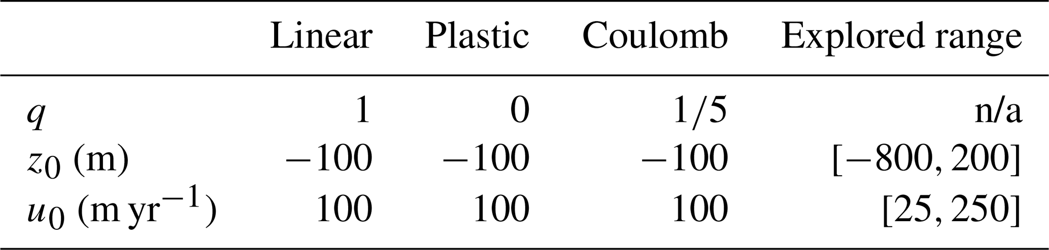
Finally, we sampled a broad parameter range of z0 values and then tuned so as to obtain an ice stream network that resembles previous mapping inventories (e.g. Fig. 2 in Margold et al., 2015). Hence, we first defined an ice stream as a set of grid points that satisfy . In other words, ice streams are defined here as regions of the ice sheet where the sliding contribution is at least 1 order of magnitude greater than ice deformation. It must be stressed that no particular LIS volume value was targeted but rather the model is tuned based on the dynamics. The same z0 value is then employed throughout the study (see Table 1). This approach provides good qualitative results and facilitates comparison among the model formulations used here.
Simulations throughout this study ran for 200 kyr to ensure a smooth equilibration from the initial state. An initial ice thickness of 1000 m is imposed over bedrock above sea level in North America above 50∘ N to urge the spin up. The necessary length of the spin-up is quantified by a two-phase linear regression (Hinkley, 1969, 1971), i.e. a statistical test for detecting a change in behaviour of a variable time series (i.e. the so-called changepoint; details in Appendix A). Namely, we applied the two-phase regression model to the ice sheet volume above flotation time series so as to determine the equilibration time (Fig. 2). The average equilibration time of all simulations presented herein reads kyr.
Thus, the first 100 kyr were assumed to represent model spin-up and are not considered in the analysis here. The remaining 50 kyr are shown in the figures below. All simulations were performed with a horizontal grid resolution of 16 km.
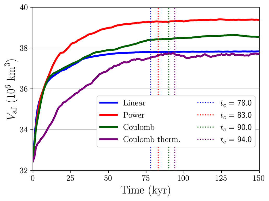
Figure 2Ice volume above flotation Vaf for the main simulations. Dashed vertical lines represent the changepoint (i.e. the transition from transitory to stationary regime) for each time series as determined by the two-phase linear regression (details in Appendix A). For t>tc, a constant equilibrium volume is reached in all cases.
Two main experiments were performed throughout this study accounting for each effective pressure formulation: purely mechanical friction (overburden) and thermomechanically coupled friction (i.e. a water-dependent parametrisation), as described above. Each of these cases is described in the following sections.
In general, our simulations largely agree in extent with prior reconstructions (Stokes et al., 2016; Stokes, 2017). This result is not expected a priori since we tuned the Yelmo ice sheet model to obtain a fully developed ice stream network (e.g. Margold et al., 2014, 2015) rather than to match a certain volume and extent estimation (Sect. 2.5). It is worth noting that Margold et al. (2015) already stressed that no inferences on the timing of ice stream operation at the LGM are possible because only a small number of the mapped ice streams have any chronological control. Rather, their mapped ice stream tracks represent a time-transgressive imprint of evolving ice stream trajectories; i.e. they cannot have all operated at once. Nonetheless, some broad spatial patterns appear, and we further exploit this fact to compare our simulations. Potential timing inconsistencies are thus inevitable, though the time-transgressive inventory remains an appropriate reference for the simulated ice streams.
Further comparison with the ice stream inventories of Margold et al. (2014) was performed by re-projecting their data to the same coordinate system used in Yelmo LIS simulations, namely, from a Lambert conformal conic projection (EPSG:3978) to polar stereographic projection.
As we shall note, the particular basal friction dependency on the sliding velocity leaves the ice extent and total volume nearly unchanged even though it strongly influences the ice stream configuration. In contrast, the thermodynamical treatment of the ice sheet base entails significant differences, mainly in total volume.
3.1 Purely mechanical friction
We first describe the reconstruction of our simulated LIS under LGM conditions for the three basal friction laws (linear, plastic and regularised Coulomb) and no thermal coupling of the basal sliding. All simulations are numerically stable and reach constant equilibrium values within the first 100 kyr. Figure 3 shows important differences in the dynamic configuration of the ice sheet among the three cases.
In the linear case, ice streams appear to be widely distributed, far beyond the expected locations from prior reconstructions (e.g. Margold et al., 2015), thus differing from the purely plastic and regularised Coulomb scenarios (Fig. 3b and c). As a result, horizontal velocities are generally high, even far from topographic troughs, allowing for strong lateral ice advection, and both the ice thickness and the volume above flotation reach a minimum (Table 2). Rapid sliding also occurs near the margins, where the continuity equations favour ice advection partially due to a large calving term. A more comprehensive dependency of the basal stress on the sliding velocity (e.g. a plastic or a regularised Coulomb) shows that a fully developed ice stream network can be simulated even for a simple overburden formulation (Fig. 3b and c). Unlike the linear case, ice streams in the latter case are constrained spatially to lower troughs as a result of friction saturation at higher velocities (Joughin et al., 2019), allowing fast streams to develop mainly where soft sediments are assumed to enhance sliding (Eq. 9).
In terms of the ice thickness dome configuration, all reconstructions show a multi-domed configuration with two relative maxima: the eastern dome, centred over Hudson Bay, and the western dome, over Lake Claire. Nevertheless, the minimum/maximum thicknesses are found for the linear and the power law scenarios respectively whilst leaving the regularised Coulomb case as an intermediate reconstruction. This is presumably caused by a further inland penetration of the north-western ice streams in the regularised Coulomb scenario compared to the purely plastic case. For the linear friction, we find generally higher velocities in the north-west and inner LIS. This translates into a larger amount of ice advected, consequently reducing the ice equilibrium thickness (mass balance equation).
The basal friction law has implications for the thermal state of the base even in the absence of thermomechanical coupling (Fig. 1b). The LIS appears to be mostly temperate, except for the south-eastern region of the Canadian Shield. The spatial distribution of the basal temperature can be understood given that the ice sheet behaves as a thermal insulator. The nearly fully temperate base in the power law corresponds to the thickest LIS reconstruction. For the base to remain frozen two main requirements must be met: low sliding velocities (i.e. low frictional heat) and low geothermal heat flow (Fig. 1b). The former is demonstrated in Fig. 3 for all three cases, whereas a strong correlation between frozen basal regions of the LIS and minimum geothermal heat flow values (Shapiro and Ritzwoller, 2004) supports the latter.
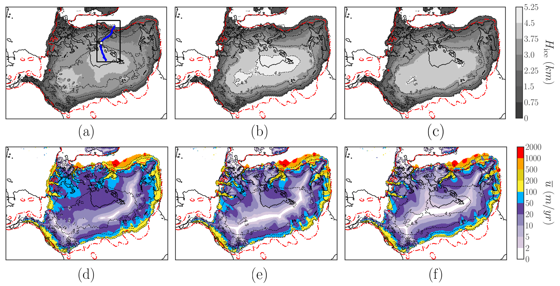
Figure 3First row: LIS ice thickness in kilometres. Second row: vertically averaged horizontal velocity. Each column corresponds to one friction law (from left to right: linear, purely plastic and regularised Coulomb). The dashed red line shows maximum reconstructed LIS extent (ICE-6G). The dashed black line shows ice thickness contours in kilometres at values of 1.0, 2.5, 3.0, 3.5, 4.0 and 4.5 km. In panel (a), the black rectangle defines the Hudson Strait subdomain as referred to in the text. A solid blue line represents the Hudson ice stream section, and a solid black contour denotes the present-day coastline. Time series evaluated over a nine-grid-point square are centred in the white dot.
Figure 5 shows that the dynamic state of the ice sheet is highly sensitive to the particular function τb(ub). We notice that the regularised Coulomb case appears to be an intermediate scenario between the linear and the purely plastic cases. However, there is a distinct common feature of the Coulomb and purely plastic cases: a linearly increasing lower boundary of τb for velocities ub>200 m yr−1. This can be explained by the minimum value of the friction coefficient (to avoid spurious velocities). This value is a constant so that the basal shear stress becomes proportional to the sliding velocity, thus giving rise to a linear dependency. The behaviour is only visible for high velocities given the nature of minimum shear stress.
From an energy balance perspective, the dissipated frictional heat Q provides an idea of how the mechanical energy is distributed in the system (Fig. 6). Our simulations have attained a steady state so all the energy that enters our system must be dissipated. The ice mass moves as a consequence of its own weight; i.e. the potential energy transfers to kinetic energy via the surface elevation slope (driving stress). The equilibrium velocity field is then maintained by the new ice accumulated on the domain. In the linear case, most of the kinetic energy is dissipated by thin ice with relatively large shear stresses. The purely plastic scenario yields a more distributed energy dissipation, where thick ice (H>3.0 km) also has a significant contribution. As mentioned before, the Coulomb case appears as an intermediate physical description, and thin ice dissipates more heat compared to the purely plastic scenario, yet large thicknesses have a significant frictional heat unlike in the linear case.
The basal stress distribution for different ice thicknesses (Fig. 5) may seem counterintuitive given that, for a fixed velocity, lower τb values are generally reached for thicker grid points. Yet this can be understood in terms of the bedrock characteristics (Eq. 8) as follows. Thick ice within the LIS is unable to reach high velocities unless it is restricted to low elevations (as cb approaches its minimum). In contrast, if we consider low thicknesses, the same velocities can be found for considerably higher cb values (since N=ρgH is smaller). In other words, for a particular velocity, thinner ice yields higher basal stress due to the bedrock characteristics.
The different ice sheet dynamics result in different configurations for the LIS (Table 2). In general, our simulations are consistent with our current knowledge of the LIS during the LGM, yet it is worth noting certain aspects of each parametrisation. The fact that the linear law leads to the lowest values of ice volume (above flotation) and ice thickness can be explained by recalling Joughin et al. (2019). For low velocities (i.e. the centre of the LIS), the linear friction law (Fig. 4d) yields lower τb values than a plastic/Coulomb law (Fig. 4e and f). Such inland points consequently have higher velocities, thus advecting ice towards the margins and decreasing the equilibrium ice thickness. This entails a straightforward reduction in the effective pressure N. As a result, the basal friction coefficient reaches a minimum. In contrast, only minor differences in ice volume are found between the more comprehensive plastic law and regularised Coulomb parametrisations.

Figure 4Homologous ice sheet base temperature (∘C) and shear stress τb (kPa) for the three friction laws: (a) linear, (b) purely plastic and (c) regularised Coulomb. The dashed red line shows maximum reconstructed LIS extent (ICE-6G). The dashed black line shows ice thickness contours in kilometres.
Lastly, we present longitudinal sections of the Hudson Strait ice stream for the linear, the purely plastic and the regularised Coulomb friction laws (Fig. 7). The location of the points of the section was selected on the basis of a maximum velocity criterion so that the section lies in the centre of the ice stream and extends from Hudson Bay to the grounding line (Fig. 3a). As we would expect, results with a linear friction law differ most. Particularly, deformation velocities close to the margin are the highest among the three laws herein, which is considered to be a result of an absent upper bound in the basal shear stress. Basal velocities near the dome of the LIS are also higher for a linear case given that τb(ub) approaches zero more rapidly for q=1 than for q<1 (Eq. 6). Therefore, the ice thickness is a minimum as dictated by the continuity equation (consistent with Table 2). A subtle difference between the power law and the regularised Coulomb case is visible on the surface elevation slope. In general, and particularly near the dome, the slope is slightly steeper in the power law case, and the consequences are noticed in a higher deformation velocity (dashed blue line) in Fig. 7b than c.
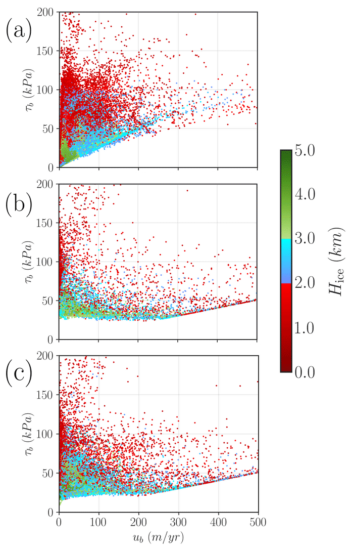
Figure 5Scatterplot of τb(ub) phase space for three different basal friction laws: (a) linear, (b) purely plastic and (c) regularised Coulomb. Every dot represents a pair (ub, τb) evaluated in a single grid point.
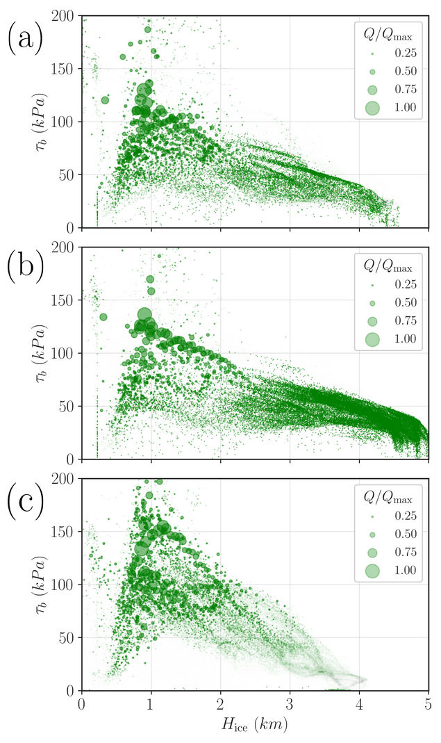
Figure 6Frictional heat distribution as a scatterplot of τb(Hice) for three different basal friction laws: (a) linear, (b) purely plastic and (c) regularised Coulomb. Every dot represents a pair (Hice,τb) evaluated in a single grid point. The marker size represents the normalised frictional heat , where Q=ubτb, and Qmax is the maximum value of each simulation.
Table 2Ice volume above flotation V, extent A, maximum ice thickness Hmax, spatially averaged basal temperature and sliding velocity for the three friction parametrisations under consideration. Standard deviation values σ are given between parentheses for averaged quantities.
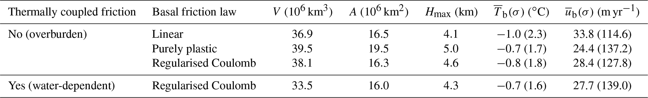
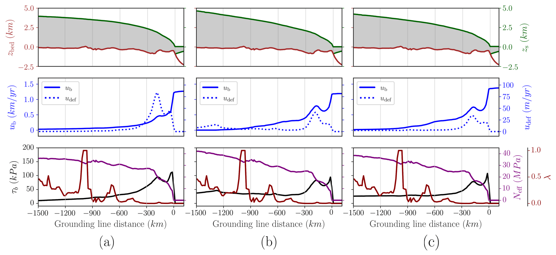
Figure 7Section along Hudson Strait ice stream (as noted in Fig. 3a) for purely mechanical basal friction: linear, purely plastic and regularised Coulomb. Green: LIS surface elevation; brown: bedrock height; blue: horizontal velocity (sliding and deformation contributions); purple: effective pressure; black: basal shear stress.
3.2 Thermomechanically coupled friction
Next we investigate the effect of coupling basal friction to the thermal state of the base by comparing the simulated LIS under LGM conditions for the water-dependent parametrisation with the purely mechanical friction formulation. A regularised Coulomb friction law is employed throughout this section. In terms of ice thickness, there is no clear distinction between a purely mechanical friction approach (Fig. 3c) and the thermomechanically coupled case (Fig. 9a) besides a minor decrease. More precisely, Table 2 shows slight differences in total ice volume and extent: the thermomechanically coupled simulations show a smaller extent and therefore a lower volume given that the ice thickness remains nearly identical. Nevertheless, such a decrease brings our simulation closer to previous reconstructions (Fig. 8), but the ice extent remains in the upper limit compared to prior studies. This further suggests that, for our particular parameter choice, a thermomechanically coupled friction may be necessary to obtain a realistic LIS extent.
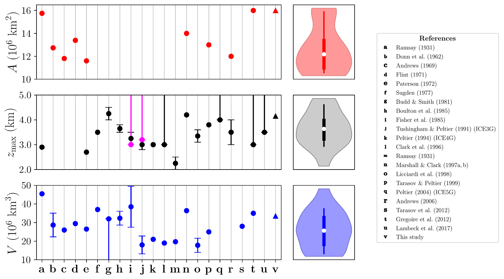
Figure 8Comparison of reconstructed LIS ice extent, maximum elevation and volume. Estimates from this study are given by triangle markers. Magenta dots show maximum ice sheet elevation for the soft bed models.
It is illustrative to build a streaming mask to perform a qualitative comparison among parametrisations as well as previous inventories (e.g. Margold et al., 2015). We therefore define sliding regions as those points that satisfy the condition , thus ensuring that ice flow due to deformation is at least 1 order of magnitude lower than the sliding contribution. In terms of this streaming mask (Fig. 9a), we generally simulate the most significant ice streams present in recent mapping inventories and comprehensive reviews of the LIS (e.g. Margold et al., 2014, 2015).
The thermomechanically coupled friction formulation entails fundamental changes in the LIS configuration and thermal state of the base. A direct inspection of Fig. 3c as compared to Fig. 9a further shows the implications in the simulated ice stream configuration, and notable improvement is found in the Hudson Strait ice stream and tributary.
The probability density functions P(ub) and P(Tb) (Fig. 10) further explore the differences among friction law formulations for both an overburden and a water-dependent effective pressure. For the linear law, we find the coldest ice base on average (see Table 2) as the tail of the distribution reaches the leftmost values compared to a power or Coulomb formulation. Notably, these last two friction laws show minor differences in terms of P(ub) and P(Tb), showing physically equivalent reconstructions in terms of probability densities. In contrast, when the basal friction is coupled with thermodynamics via Eq. (11), we note a shift towards higher velocities P(ub) for low velocities (i.e. ub<250 m yr−1), thus implying a speed-up of the slower regions of the ice sheet. Consequently, the outflow of ice becomes larger, and the equilibrium thickness is reduced compared to the Coulomb overburden scenario (Table 2).
When the basal friction is thermomechanically coupled (Table 2), the LIS extent is reduced, and the maximum ice thickness is lower, leading to a smaller equilibrium volume. This is explained through the decrease in basal friction. In this case, there is an additional degree of freedom that may yield a reduction in basal friction: the effective pressure. All temperate grid points undergo a reduction in their effective pressure (and consequently in the basal stress) by up to a 10 % of their original value. As a result, the stress balance will yield higher velocities and a lower equilibrium thickness for a fixed set of boundary conditions. In contrast, in the purely mechanical friction case, the value of cb is determined solely by the bedrock elevation, which does not change significantly over the course of the experiment.
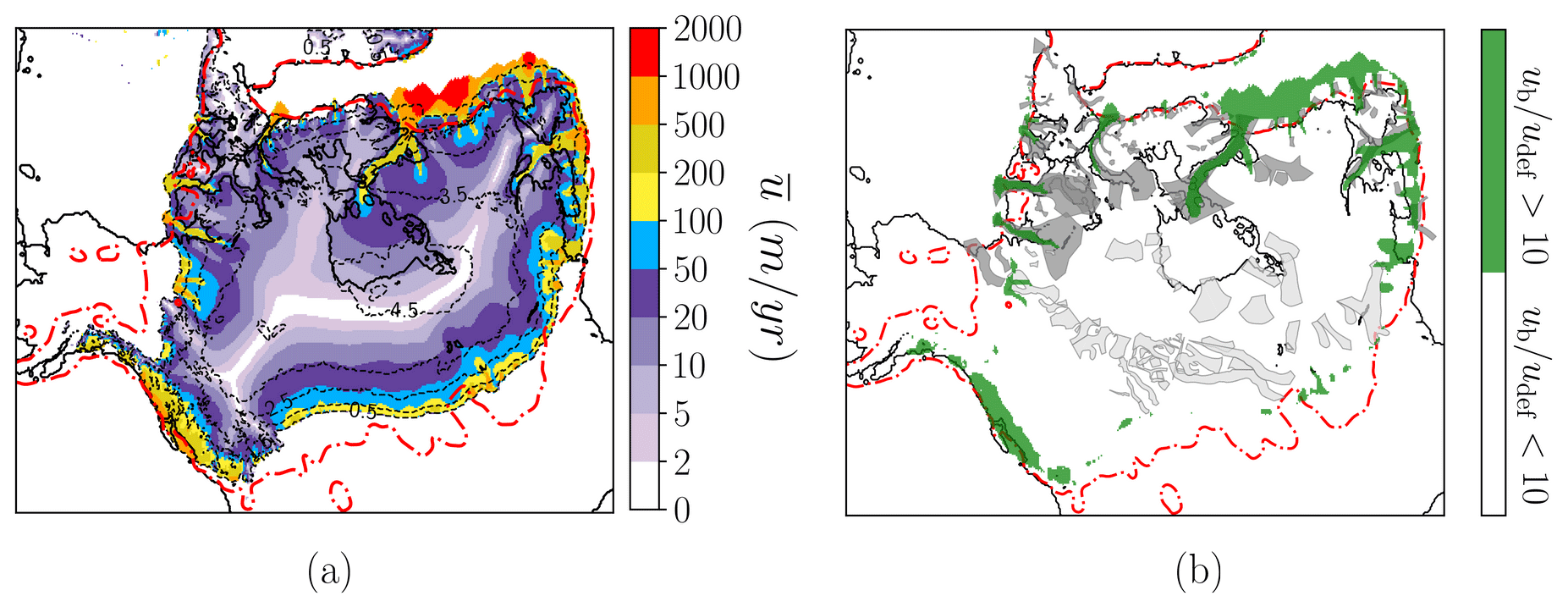
Figure 9(a) LIS depth-averaged horizontal velocity, (b) spatial mask (green) depicting the two ice flow regimes overlaid with the ice stream inventory of Margold et al. (2014) (polygons). Solid polygons correspond to land-terminating (light gray) and marine-terminating (dark gray) ice streams respectively. Streaming grid points meet the condition so that the flow due to ice deformation represents, at highest, a contribution 1 order of magnitude below sliding. Both fields are shown for a water-dependent effective pressure. The dashed red line shows maximum reconstructed LIS extent (ICE-6G). The dashed black line shows ice thickness contours of 1.0, 2.5, 3.0, 3.5, 4.0 and 4.5 km.
Nevertheless, the equilibrium volume, relevant for the sea-level contribution, does not encapsulate all the relevant information about the LIS, especially for the Hudson subdomain. Notably, the ice volume in the Hudson subdomain (as defined by the black rectangle in Fig. 3a) reaches a constant equilibrium value in both the purely mechanical and thermomechanically coupled experiments. Likewise, the vertically averaged horizontal velocity also attains a constant value, yet slightly higher due to the water-dependent effective pressure for the aforementioned mechanism.
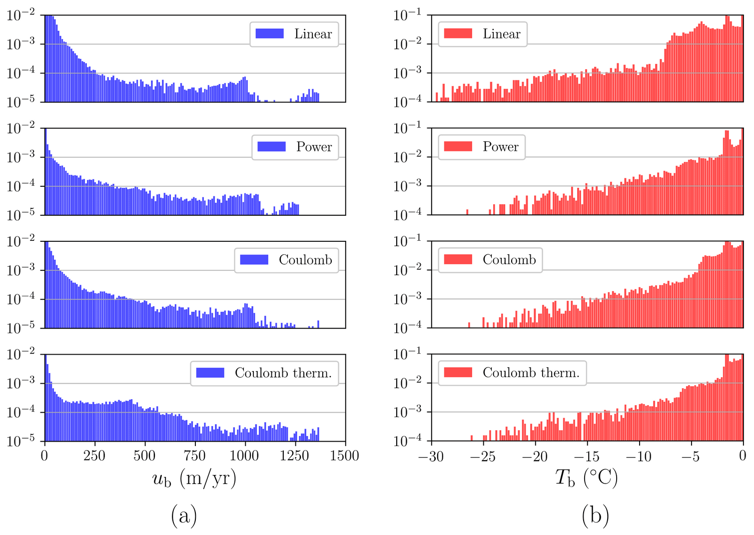
Figure 10Probability density functions (PDFs) of (a) log10P(ub) and (b) log10P(Tb). Each row represents a different friction formulation. From top to bottom: linear, power law, regularised Coulomb and regularised Coulomb with a water-dependent effective pressure formulation. Note the difference in y-axis limits.
Global variables such as the total LIS volume are not the only ones that undergo changes when the basal friction is further coupled to thermodynamics. This result is captured by Fig. 11a. Unlike its counterpart in the purely mechanical case (Fig. 5a), we find an interesting behaviour of the non-monotonic minimum shear stress values in the low-velocity regime (ub<150 m yr−1) when the basal friction is coupled with thermodynamics. Nonetheless, all points taking part in this minimum shear stress region correspond to a fully drained till. Hence, explicit water changes do not explain the difference in behaviour. Presumably, we argue that those points with the lowest τb cannot be reached given that the new stress balance (i.e. the shallow shelf approximation, SSA, equations) is changed if we account for Neff. Since the SSA solution is non-local, the particular shape of τb(ub) can be modified by a water-dependent effective pressure even for regions that are fully drained. This implicit effect would be a direct consequence of the non-local nature of the SSA solutions in regions where the water content remains constant.
It is also illustrative to compare the Coulomb friction law for both a purely mechanical friction and the thermomechanically coupled case from a frictional heat perspective (Fig. 6c and c respectively). When the basal friction is then coupled with the thermal state of the base via a water layer thickness Hw, we notice two main changes. First, the shear stress values are generally reduced, and the thicker regions of the LIS contribute more to frictional heat dissipation (larger region covered in green for H>3.0 km).
It is clear from Fig. 11b that, for an effective pressure that depends on basal water thickness, sliding occurs when the till is saturated in water. This requires a sustained supply of heat (e.g. basal frictional heat, geothermal heat flow) to melt enough water so as to keep a saturated till, thus surpassing the drainage rate and eluding refreezing (due to heat diffusion–advection, Eq. 1). This is unlikely to occur in the central region of the ice sheet, where neither low troughs nor high surface slopes are present, consequently yielding low driving stresses and basal frictional heat.
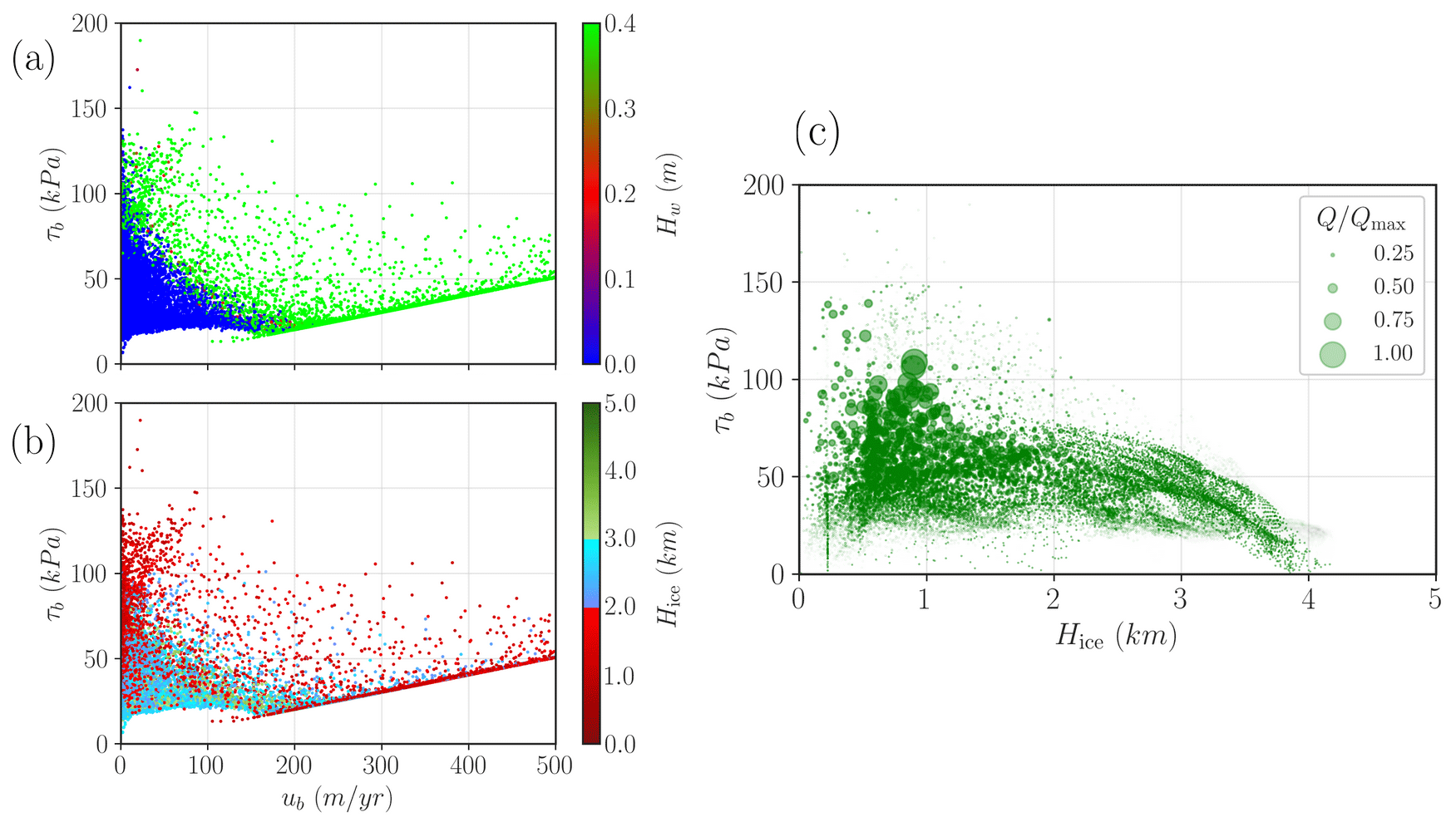
Figure 11Scatterplot of τb(ub) phase space for the water-dependent effective pressure formulation, coloured according to (a) ice thickness and (b) basal water content. Every dot represents a pair (ub,τb) evaluated in a single grid point. Panel (c) shows a scatterplot of τb(Hice) for the water-dependent effective pressure, where each dot represents a pair (H,τb) evaluated in a single grid point. The marker size depicts the normalised frictional heat , where Qmax is the maximum frictional heat value.
In general, the ice sheets simulated herein are consistent with our knowledge of the LGM Laurentide Ice Sheet state. Qualitatively, this can be seen by a comparison of Fig. 9b with previous reconstructions of LIS ice dynamics (e.g. Margold et al., 2015; Stokes et al., 2016). Notably, the main ice streams of the LIS (i.e. Amundsen Gulf, M'Clure Strait, Massey Sound, Gulf of Boothia, Lancaster Sound and Hudson Strait) are present in our simulation even in the absence of thermomechanical coupling (Fig. 3b and c). However, both the configuration of ice streams and the total ice sheet volume are found to be strongly dependent on the basal friction formulation.
In particular, the linear basal friction law clearly yields significantly lower shear stress values compared to the other formulations (Fig. 3). Despite the fact that both ice extent and volume do not fall far from previous studies, relatively high velocities are found further inland in ice streams along the northern LIS and are not fully constrained to lower troughs (Fig. 3a). As a result, the ice sheet under this parametrisation exhibits a minimum volume and a simple-domed ice sheet that resembles past reconstructions that ignore deformable beds (e.g. Denton and Hughes, 1981). This can be understood as follows. The equilibrium thickness is in fact explicitly dependent on the horizontal velocity via the continuity equation, thus reaching a minimum value when the velocity is high for a fixed set of boundary conditions (i.e. the accumulation rate). Hence, the maximum ice thickness yields its lowest value in this reconstruction.
These results could lead to the hypothesis that rapid ice streaming spatially constrained to lower troughs requires a thermal coupling with the base. Nevertheless, the absence of a thermomechanical coupling solely exhibits a fully developed and spatially constrained ice stream structure when a more realistic function for τb(ub) is provided (i.e. a power law or a regularised Coulomb). Although the same ice extent appears to be reached independent of such a function, it closely matches the ICE-6G reconstruction. Thus, thermomechanical coupling is not necessary to simulate a fully developed ice stream network in the expected locations. In fact, a more realistic τb(ub) is sufficient to find rapid streaming regions spatially constrained to low troughs, as is the case for a purely plastic or a regularised Coulomb parametrisation. Significantly lower basal friction values are yielded by the former, yet the dynamic configuration of the ice sheet seems almost identical. Despite these similarities, from a purely thermodynamic perspective of the ice sheet base, the choice of τb(ub) is fundamental even when thermal coupling is not considered. This is presumably due to the insulator effect of a thicker ice sheet from the colder atmosphere (see maximum equilibrium thickness in Table 2).
Fundamental changes are noticed when the basal friction parametrisation is coupled with the thermal state of the base (Figs. 10 and 11). Rapidly flowing ice streams are present in expected locations, such as through Hudson Strait, Amundsen Gulf, M'Clure Strait, Lancaster Sound and Gulf of St Lawrence (Margold et al., 2015). Consequently, both the total volume and the equilibrium ice thickness are reduced. Overall, the simulated ice sheet closely matches the reconstructed ICE-6G extent, even though it is somewhat lower than for the overburden case. All friction laws presented herein yield a multi-domed ice sheet where two independent domes are found (western and eastern) irrespective of the thermomechanical coupling. The total ice volume, in terms of contribution above flotation, is 33.5×10⁶ km3 (Table 2). This value is larger than the estimate given by Tarasov et al. (2012) ( km3), though close to Gregoire et al. (2012) (35×106 km3). Furthermore, no large volume changes are found in either the entire LIS or the Hudson region that would resemble binge–purge oscillations (MacAyeal, 1993a).
Not only does the Bueler and van Pelt (2015) effective pressure formulation couple ice dynamics with the thermomechanical state of the base, but also the amount of liquid water is considered to compute the effective pressure. Figure 5 shows a significant difference in terms of the horizontal velocity and the basal friction coefficient. As described above, the simulated ice sheet also appears to be a multi-domed configuration with two relative maxima that resemble the previous result (western and eastern domes). Even so, the ice stream structure strongly differs from the purely mechanical friction approach. First, the ice streams are more restricted spatially, in the sense that they do not propagate as far inland. Second, even for non-streaming regions, τb values are generally higher for the water-dependent effective pressure formulation.
The fact that all our reconstructions share a multi-domed equilibrium configuration resembles the prevailing approach of LIS reconstructions that have accounted for lubricated basal conditions, in which the ice sheet over Hudson Bay was consequently thinner and less steeply sloped (e.g. Boulton et al., 1985; Fisher et al., 1985). Nonetheless, the surface elevation over Hudson Bay was substantially lower in those cases, with a maximum elevation above present sea level of 3.0–3.5 km, in contrast to our ∼4–5 km thickness. This comparison must be taken with caution since surface elevation and ice thickness do not represent the same magnitude. Yet, it is possible to have an approximate comparison among reconstructions by also looking at the volume differences. Boulton et al. (1985) span a volume of 33–44×106 km3, substantially larger than the 21.1–25.9×10⁶ km3 range of Fisher et al. (1985) for the hard bed model in both cases (Fig. 8). Our particular volume values fall within the range of Boulton et al. (1985). In terms of volume and ice extent, results from the water-dependent effective pressure formulation yield a slightly larger ice volume as a result of narrower and shorter ice streams that consequently advect less ice towards the margins. This dynamic distinction is significant for ice extent given that the reconstructions exhibit the lowest ice extent value (16.0×10⁶ km2).
Notably, the most realistic parametrisation (a water-dependent effective pressure formulation) shows an interesting behaviour that deviates from the cases using the overburden pressure approach. For low velocities, the shape of τb(ub) is almost identical to the overburden case. Nevertheless, for higher velocities (ub>80 m yr−1), the phase space τb(ub) differs from the purely mechanical reconstructions, where quite low basal stresses are yielded. Figure 11a and b then establish the distribution of ice thickness and basal water content throughout the ice sheet. In terms of the former (Fig. 11a), fast sliding occurs in grid points with a medium-sized thickness (1.0–3.0 km), exhibiting a perfect correlation with water-saturated grid points (Fig. 11b).
In a somewhat more realistic approach to basal friction, we must consider the additional dependency on the effective pressure τb(ub,Neff), thus triggering rapid ice streaming in temperate regions. Nevertheless, the assumption that ice streaming occurs in all temperate grid points leads to an extremely low shear stress in the centre of the ice sheet (Fig. 5). For this reason, accounting for hydrological processes (e.g. the basal water content) appears to be fundamental to simulate Laurentide ice streams in accordance with geological reconstructions (Margold et al., 2015) and further yields ice sheet volume and maximum elevation values closer to prior studies (Fig. 8). Moreover, a water-dependent friction substantially considers the thermal state of the base, rather than just local dynamics. This implies a stress balance influenced by the geothermal heat flux as well as the frictional and deformation heat contributions.
Overall, the simulated ice streams are numerically well behaved and spatially constrained to lower troughs. In general, horizontal velocities reach an equilibrium value once the ice sheet has stabilised. However, global LIS variables such as the total ice volume are highly sensitive to both the choice of friction law and the thermal coupling at the base.
We have simulated the LIS under LGM boundary conditions considering three basal friction scenarios of varying dynamic complexity and their consequences for the LIS ice streams, configuration, extent and volume.
First, in the purely mechanical friction formulation, we solely accounted for the force exerted by the weight of the ice column on a given grid point (overburden pressure). In this context, we considered three different dependencies of the basal shear stress on the sliding velocity: linear, purely plastic and regularised Coulomb. Friction was thus independent of the thermal state of the base. The LIS extent closely matches the reconstructed ICE 6G ice sheet, yet the volume appears to be slightly larger. For the linear case, this is a consequence of the absence of an active ice stream network spatially constrained to low troughs that advects ice from the centre of the ice sheet to the margins. The surface elevation reflects a simple-domed ice sheet (except for the regularised Coulomb scenario) resembling past results where the LIS deformable bedrock was ignored. Remarkably, a fully developed ice stream network was simulated for a purely plastic and regularised Coulomb formulation without any thermomechanical coupling requirements, yet the equilibrium ice volume appears to be slightly larger than previous reconstructions.
Hydrological processes were considered by coupling the basal friction to the thermal state of the base via the implementation of a water-dependent effective pressure formulation (Bueler and van Pelt, 2015). The simulated ice sheet also appears to be a multi-domed configuration with two relative maxima, yet the ice stream structure strongly differs from the overburden approach for two reasons. First, the ice streams are spatially more restricted, and second, the basal friction coefficient is generally higher for non-streaming regions. This approach yields the closest ice sheet volume to prior LIS reconstructions that also consider fast sliding in regions of a lubricated bed. These results support the hypothesis that hydrological processes are necessary to achieve physical realism in our simulations and to obtain realistic ice volume reconstructions similar to previous work.
Notably, ice volume above flotation reached a constant equilibrium value for all the cases under consideration. Precise values are highly sensitive to thermomechanical coupling of the basal friction. The overburden case seems to overestimate the LIS volume compared to previous reconstructions. Nevertheless, significantly lower values are simulated when the thermal state of the base is accounted for, yet the particular coupling parametrisation does not exhibit significant changes regarding ice volume or total ice sheet extent. A water-dependent formulation yields volume and ice extent values substantially closer to prior studies.
Lastly, we can conclude that the most sophisticated scenario in this work (a thermomechanically coupled regularised Coulomb basal friction) appears to be the reconstruction closest to reality compared to previous ice stream inventories. Future experiments shall focus on a more realistic basal hydrology, where conservative non-local processes (as the horizontal advection) are also resolved.
The two-phase linear regression model was studied by Hinkley (1969, 1971) and later also applied by Solow (1987). For our purpose, the underlying idea is to determine the changepoint in a given time series y(t) to estimate the necessary length of the equilibration time in our simulations. Conceptually, the two-phase regression model assumes that there are two different behaviours in our data, and these are captured by two independent linear functions (Eq. A1). In the present study, these behaviours correspond to the transitory and stationary nature of the solutions respectively. The changepoint is thus defined as the abscissa of the intersection that minimises the residual sum of squares. Mathematically, we can write this model as
where the abscissa of the intersection of these two regression lines reads
and it is referred to as the changepoint.
Following Solow (1987), for our changepoint definition, we must ensure continuity of the underlying time series by imposing tc to lie in the interval . Otherwise, the two-phase regression will include a discontinuity at tc.
The approach thus aims at finding the estimate tc. Since no closed form expression of tc is possible, the model given by Eq. (A1) is usually rewritten as
where εi is the error term, , and Ωi(c) is given by
Fixing a value of c, the modified model in Eq. (A3) becomes a standard linear regression with two regressor variables: ti and ti−c. Our problem is now reduced to finding tc so that its value minimises the residual sum of squares (Fig. A1). For large datasets, Hinkley (1971) provides a description of an efficient algorithm, though we simply apply a direct grid search given the dimensions of our time series.
Particularly, we used the ice volume above sea level as the regressand and performed the calculations previously described. The dashed vertical line in Fig. 2 represent the abscissa of the changepoint tc. Solow (1987) determines such a value by minimising the residual sum of squares (RSS), though we additionally compare these results with those given by maximising the determination coefficient (R2) (Fig. A1). The values yielded by each method coincide.
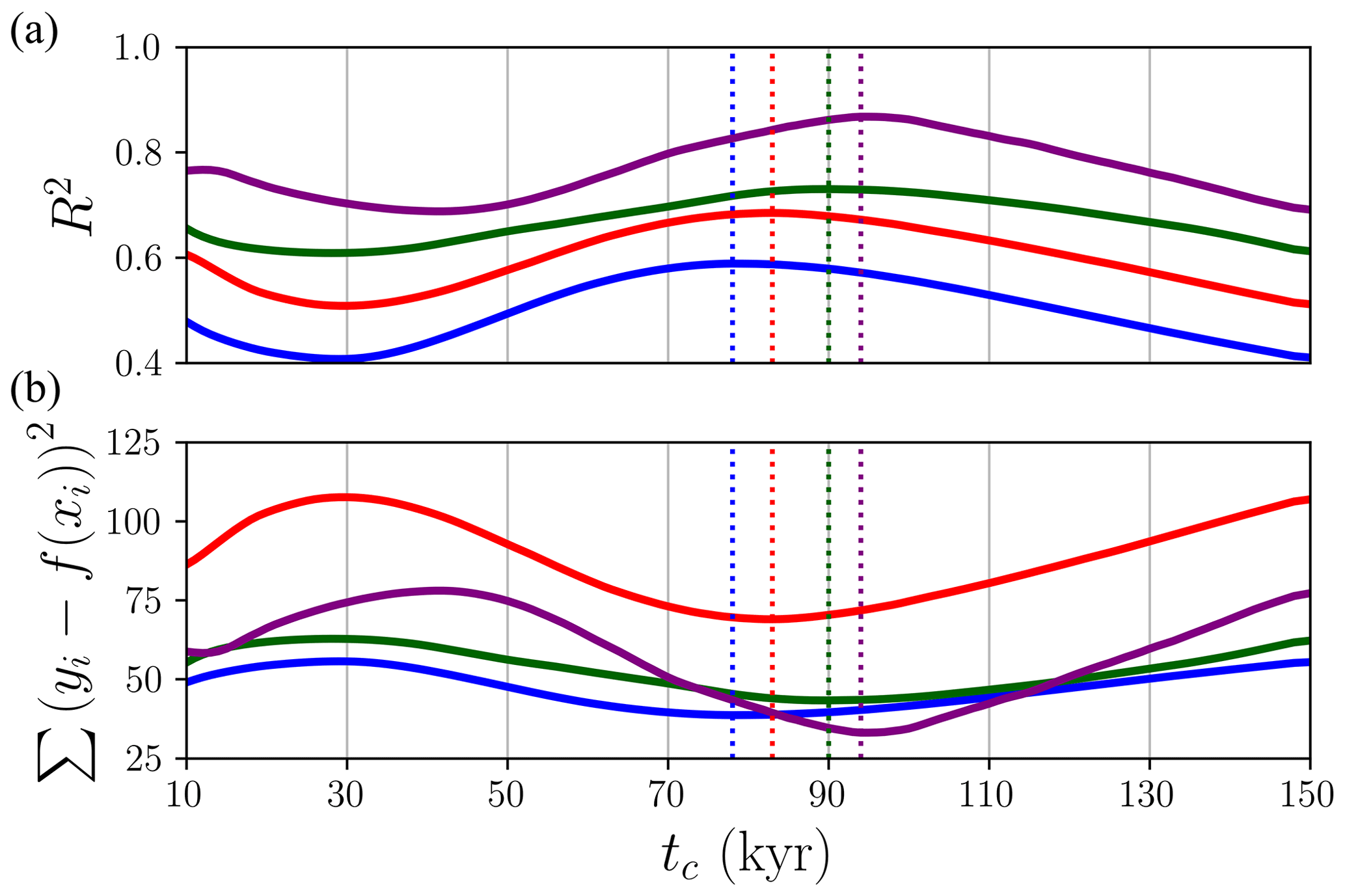
Figure A1Determination coefficient (R2) (a) and residual sum of squares (RSS) (b) as a function of the fixed changepoint value taken. For each tc value, a standard linear regression (Eq. A3) with two regressor variables is performed using the volume above sea level as a regressand. The dashed vertical lines correspond to the maximum and minimum values of R2 and RSS respectively.
Code to make all plots herein present and additional calculations is available in an open Github repository: https://github.com/d-morenop/Laurentide-ice-sheet-LGM (last access: 5 May 2023; DOI: https://doi.org/10.5281/zenodo.7908212, Moreno-Parada et al., 2023b). Yelmo ice sheet model code is additionally available at https://github.com/palma-ice/yelmo (Robinson et al., 2020). Model output is available at a persistent Zenodo repository at https://doi.org/10.5281/zenodo.7892395 (Moreno-Parada et al., 2023a).
DMP ran all the simulations, analysed the results and wrote the paper. All other authors contributed to the analysis of the results and writing of the paper.
At least one of the (co-)authors is a member of the editorial board of The Cryosphere. The peer-review process was guided by an independent editor, and the authors also have no other competing interests to declare.
Publisher's note: Copernicus Publications remains neutral with regard to jurisdictional claims in published maps and institutional affiliations.
We thank Félix Garcia-Pereira for suggesting the two-phase regression method to determine the equilibration time. We are grateful to Julien Seguinot, Niall Gandy and the editor Chris R. Stokes for their comments, which have greatly improved our paper.
This research has been supported by the Spanish Ministry of Science and Innovation (project IceAge, grant no. PID2019-110714RA-100) and the Ramón y Cajal programme of the Spanish Ministry of Science and Innovation and the Spanish Ministry of Universities (grant no. RYC-2016-20587). This research is TiPES contribution no. 183 and has been supported by the European Union Horizon 2020 research and innovation programme (grant no. 820970).
This paper was edited by Chris R. Stokes and reviewed by Julien Seguinot and Niall Gandy.
Albrecht, T., Winkelmann, R., and Levermann, A.: Glacial-cycle simulations of the Antarctic Ice Sheet with the Parallel Ice Sheet Model (PISM) – Part 2: Parameter ensemble analysis, The Cryosphere, 14, 633–656, https://doi.org/10.5194/tc-14-633-2020, 2020. a, b
Alley, R.: K.M. Cuffey and W.S.B. Paterson. 2010. The physics of glaciers. Fourth edition. Amsterdam, etc., Academic Press. 704pp. ISBN-10: 0-123694-61-2, ISBN-13: 978-0-123-69461-4, hardback,, J. Glaciol., 57, 383–384, https://doi.org/10.3189/002214311796405906, 2011. a
Aschwanden, A., Aðalgeirsdóttir, G., and Khroulev, C.: Hindcasting to measure ice sheet model sensitivity to initial states, The Cryosphere, 7, 1083–1093, https://doi.org/10.5194/tc-7-1083-2013, 2013. a
Blasco, J., Alvarez-Solas, J., Robinson, A., and Montoya, M.: Exploring the impact of atmospheric forcing and basal drag on the Antarctic Ice Sheet under Last Glacial Maximum conditions, The Cryosphere, 15, 215–231, https://doi.org/10.5194/tc-15-215-2021, 2021. a
Blatter, H.: Velocity and stress fields in grounded glaciers: a simple algorithm for including deviatoric stress gradients, J. Glaciol., 41, 333–344, https://doi.org/10.3189/s002214300001621x, 1995. a
Boulton, G. and Hagdorn, M.: Glaciology of the British Isles Ice Sheet during the last glacial cycle: form, flow, streams and lobes, Quaternary Sci. Rev., 25, 3359–3390, https://doi.org/10.1016/j.quascirev.2006.10.013, 2006. a
Boulton, G. S., Smith, G. D., Jones, A. S., and Newsome, J.: Glacial geology and glaciology of the last mid-latitude ice sheets, J. Geol. Soc., 142, 447–474, https://doi.org/10.1144/gsjgs.142.3.0447, 1985. a, b, c, d
Brocq, A. L., Payne, A., Siegert, M., and Alley, R.: A subglacial water-flow model for West Antarctica, J. Glaciol., 55, 879–888, https://doi.org/10.3189/002214309790152564, 2009. a
Bueler, E. and Brown, J.: Shallow shelf approximation as a “sliding law” in a thermomechanically coupled ice sheet model, J. Geophys. Res, 114, F03008, https://doi.org/10.1029/2008JF001179, 2009. a
Bueler, E. and van Pelt, W.: Mass-conserving subglacial hydrology in the Parallel Ice Sheet Model version 0.6, Geosci. Model Dev., 8, 1613–1635, https://doi.org/10.5194/gmd-8-1613-2015, 2015. a, b, c, d, e, f, g
Calov, R., Ganopolski, A., Petoukhov, V., Claussen, M., and Greve, R.: Large-scale instabilities of the Laurentide ice sheet simulated in a fully coupled climate-system model, Geophys. Res. Lett., 29, 2216, https://doi.org/10.1029/2002gl016078, 2002. a
Clark, J. A.: The reconstruction of the Laurentide Ice Sheet of North America from sea level data: Method and preliminary results, J. Geophys. Res.-Sol. Ea., 85, 4307–4323, https://doi.org/10.1029/jb085ib08p04307, 1980. a, b
Denton, G. H. and Hughes, T. J.: The Last Great Ice Sheets, Wiley Interscience, New York, p. 484, 1981. a, b
Dyke, A., Andrews, J., Clark, P., England, J., Miller, G., Shaw, J., and Veillette, J.: The Laurentide and Innuitian ice sheets during the Last Glacial Maximum, Quaternary Sci. Rev., 21, 9–31, https://doi.org/10.1016/s0277-3791(01)00095-6, 2002. a
Fisher, D. A., Reeh, N., and Langley, K.: Objective Reconstructions of the Late Wisconsinan Laurentide Ice Sheet and the Significance of Deformable Beds, Géogr. Phys. Quatern., 39, 229–238, https://doi.org/10.7202/032605ar, 1985. a, b, c
Goldberg, D. N.: A variationally derived, depth-integrated approximation to a higher-order glaciological flow model, J. Glaciol., 57, 157–170, https://doi.org/10.3189/002214311795306763, 2011. a
Gowan, E. J., Zhang, X., Khosravi, S., Rovere, A., Stocchi, P., Hughes, A. L. C., Gyllencreutz, R., Mangerud, J., Svendsen, J.-I., and Lohmann, G.: A new global ice sheet reconstruction for the past 80 000 years, Nat. Commun., 12, 1199, https://doi.org/10.1038/s41467-021-21469-w, 2021. a
Gregoire, L. J., Payne, A. J., and Valdes, P. J.: Deglacial rapid sea level rises caused by ice-sheet saddle collapses, Nature, 487, 219–222, https://doi.org/10.1038/nature11257, 2012. a, b
Hinkley, D. V.: Inference about the intersection in two-phase regression, Biometrika, 56, 495–504, https://doi.org/10.1093/biomet/56.3.495, 1969. a, b
Hinkley, D. V.: Inference in Two-Phase Regression, J. Am. Stat. Assoc., 66, 736–743, https://doi.org/10.1080/01621459.1971.10482337, 1971. a, b, c
Hooke, R. L.: Principles of Glacier Mechanics, Cambridge University Press, https://doi.org/10.1017/cbo9780511614231, 2005. a
Hughes, T., Denton, G. H., Anderson, B. G., Schilling, D. H., Fastook, J. L., and Lingle, C.: The last great ice sheets: A global view, edited by: Denton, G. H. and Hughes, T., 1980. a
Jenssen, D.: A Three-Dimensional Polar Ice-Sheet Model, J. Glaciol., 18, 373–389, https://doi.org/10.3189/s0022143000021067, 1977. a
Joughin, I., Smith, B. E., and Schoof, C. G.: Regularized Coulomb Friction Laws for Ice Sheet Sliding: Application to Pine Island Glacier, Antarctica, Geophys. Res. Lett., 46, 4764–4771, https://doi.org/10.1029/2019gl082526, 2019. a, b, c, d
Kleman, J., Hättestrand, C., Borgström, I., and Stroeven, A.: Fennoscandian palaeoglaciology reconstructed using a glacial geological inversion model, J. Glaciol., 43, 283–299, https://doi.org/10.1017/s0022143000003233, 1997. a
Lipscomb, W. H., Price, S. F., Hoffman, M. J., Leguy, G. R., Bennett, A. R., Bradley, S. L., Evans, K. J., Fyke, J. G., Kennedy, J. H., Perego, M., Ranken, D. M., Sacks, W. J., Salinger, A. G., Vargo, L. J., and Worley, P. H.: Description and evaluation of the Community Ice Sheet Model (CISM) v2.1, Geosci. Model Dev., 12, 387–424, https://doi.org/10.5194/gmd-12-387-2019, 2019. a
Ma, Y., Gagliardini, O., Ritz, C., Gillet-Chaulet, F., Durand, G., and Montagnat, M.: Enhancement factors for grounded ice and ice shelves inferred from an anisotropic ice-flow model, J. Glaciol., 56, 805–812, https://doi.org/10.3189/002214310794457209, 2010. a, b
MacAyeal, D. R.: Binge/purge oscillations of the Laurentide ice sheet as a cause of the North Atlantic's Heinrich events, Paleoceanography, 8, 775–784, 1993a. a, b
MacAyeal, D. R.: A low-order model of the Heinrich event cycle, Paleoceanography, 8, 767–773, 1993b. a
Mahaffy, M. W.: A three-dimensional numerical model of ice sheets: Tests on the Barnes Ice Cap, Northwest Territories, J. Geophys. Res., 81, 1059–1066, https://doi.org/10.1029/jc081i006p01059, 1976. a
Margold, M., Stokes, C. R., Clark, C. D., and Kleman, J.: Ice streams in the Laurentide Ice Sheet: a new mapping inventory, J. Maps, 11, 380–395, https://doi.org/10.1080/17445647.2014.912036, 2014. a, b, c, d
Margold, M., Stokes, C. R., and Clark, C. D.: Ice streams in the Laurentide Ice Sheet: Identification, characteristics and comparison to modern ice sheets, Earth-Sci. Rev., 143, 117–146, https://doi.org/10.1016/j.earscirev.2015.01.011, 2015. a, b, c, d, e, f, g, h, i
Maris, M. N. A., de Boer, B., Ligtenberg, S. R. M., Crucifix, M., van de Berg, W. J., and Oerlemans, J.: Modelling the evolution of the Antarctic ice sheet since the last interglacial, The Cryosphere, 8, 1347–1360, https://doi.org/10.5194/tc-8-1347-2014, 2014. a
Marshall, S. J., Clarke, G. K. C., Dyke, A. S., and Fisher, D. A.: Geologic and topographic controls on fast flow in the Laurentide and Cordilleran Ice Sheets, J. Geophys. Res.-Sol. Ea., 101, 17827–17839, https://doi.org/10.1029/96jb01180, 1996. a
Martin, M. A., Winkelmann, R., Haseloff, M., Albrecht, T., Bueler, E., Khroulev, C., and Levermann, A.: The Potsdam Parallel Ice Sheet Model (PISM-PIK) – Part 2: Dynamic equilibrium simulation of the Antarctic ice sheet, The Cryosphere, 5, 727–740, https://doi.org/10.5194/tc-5-727-2011, 2011. a
Meur, E. L. and Huybrechts, P.: A comparison of different ways of dealing with isostasy: examples from modelling the Antarctic ice sheet during the last glacial cycle, Ann. Glaciol., 23, 309–317, https://doi.org/10.3189/s0260305500013586, 1996. a
Moreno-Parada, D., Alvarez-Solas, J., Blasco, J., Montoya, M., and Robinson, A.: Simulating the Laurentide Ice Sheet of the LGM (Datasets from Yelmo_v1.751 output simulations) (Yelmo_v1.751), Zenodo [data set], https://doi.org/10.5281/zenodo.7892395, 2023a. a
Moreno-Parada, D., Alvarez-Solas, J., Blasco, J., Montoya, M., and Robinson, A.: d-morenop/Laurentide-ice-sheet-LGM: Laurentide Ice Sheet LGM v1.0, Zenodo [data set], https://doi.org/10.5281/zenodo.7908212, 2023b. a
Ottesen, D., Dowdeswell, J., and Rise, L.: Submarine landforms and the reconstruction of fast-flowing ice streams within a large Quaternary ice sheet: The 2500-km-long Norwegian-Svalbard margin (57∘–80∘N), Geol. Soc. Am. Bull., 117, 1033–1050, https://doi.org/10.1130/b25577.1, 2005. a
Paterson, W. S. B.: Laurentide Ice Sheet: Estimated volumes during Late Wisconsin, Rev. Geophys., 10, 885–917, https://doi.org/10.1029/rg010i004p00885, 1972. a, b
Pattyn, F.: A new three-dimensional higher-order thermomechanical ice sheet model: Basic sensitivity, ice stream development, and ice flow across subglacial lakes, J. Geophys. Res., 108, 2382, https://doi.org/10.1029/2002jb002329, 2003. a
Peltier, W.: Global glacial isostasy and the surface of the ice-age Earth- The ICE-5 G(VM 2) model and GRACE, Annu. Rev. Earth Pl. Sc., 32, 111–149, 2004. a
Peltier, W. R.: Ice Age Paleotopography, Science, 265, 195–201, https://doi.org/10.1126/science.265.5169.195, 1994. a
Peyaud, V., Ritz, C., and Krinner, G.: Modelling the Early Weichselian Eurasian Ice Sheets: role of ice shelves and influence of ice-dammed lakes, Clim. Past, 3, 375–386, https://doi.org/10.5194/cp-3-375-2007, 2007. a
Pollard, D. and DeConto, R. M.: Description of a hybrid ice sheet-shelf model, and application to Antarctica, Geosci. Model Dev., 5, 1273–1295, https://doi.org/10.5194/gmd-5-1273-2012, 2012. a
Quiquet, A., Dumas, C., Ritz, C., Peyaud, V., and Roche, D. M.: The GRISLI ice sheet model (version 2.0): calibration and validation for multi-millennial changes of the Antarctic ice sheet, Geosci. Model Dev., 11, 5003–5025, https://doi.org/10.5194/gmd-11-5003-2018, 2018. a
Ramsay, W.: Changes of sea-level resulting from the increase and decrease of glaciation, Fennia, Geographical Society of Finland, 52, 1–62, 1931. a
Ritz, C.: Time dependent boundary conditions for calculation oftemperature fields in ice sheets, The Physical Basis of Ice Sheet Modeling. International Association of Hydrological Sciences Press, Institute of Hydrology, Wallingford, Oxfordshire UK, 207–216, 1987. a
Robinson, A., Alvarez-Solas, J., Montoya, M., Goelzer, H., Greve, R., and Ritz, C.: Description and validation of the ice-sheet model Yelmo (version 1.0), Geosci. Model Dev., 13, 2805–2823, https://doi.org/10.5194/gmd-13-2805-2020, 2020 (code available at: https://github.com/palma-ice/yelmo, last acccess: 5 May 2023). a, b
Robinson, A., Goldberg, D., and Lipscomb, W. H.: A comparison of the stability and performance of depth-integrated ice-dynamics solvers, The Cryosphere, 16, 689–709, https://doi.org/10.5194/tc-16-689-2022, 2022. a
Schaffer, J., Timmermann, R., Arndt, J. E., Kristensen, S. S., Mayer, C., Morlighem, M., and Steinhage, D.: A global, high-resolution data set of ice sheet topography, cavity geometry, and ocean bathymetry, Earth Syst. Sci. Data, 8, 543–557, https://doi.org/10.5194/essd-8-543-2016, 2016. a
Schoof, C.: The effect of cavitation on glacier sliding, P. R. Soc. A, 461, 609–627, https://doi.org/10.1098/rspa.2004.1350, 2005. a
Schoof, C.: Ice-sheet acceleration driven by melt supply variability, Nature, 468, 803–806, https://doi.org/10.1038/nature09618, 2010. a
Shapiro, N. M. and Ritzwoller, M. H.: Inferring surface heat flux distributions guided by a global seismic model: particular application to Antarctica, Earth Planet. Sc. Lett., 223, 213–224, https://doi.org/10.1016/j.epsl.2004.04.011, 2004. a, b
Solow, A. R.: Testing for Climate Change: An Application of the Two-Phase Regression Model, J. Clim. Appl. Meteorol., 26, 1401–1405, https://doi.org/10.1175/1520-0450(1987)026<1401:tfccaa>2.0.co;2, 1987. a, b, c
Stokes, C.: Deglaciation of the Laurentide Ice Sheet from the Last Glacial Maximum, Cuadernos de Investigación Geográfica, 43, 377–428, https://doi.org/10.18172/cig.3237, 2017. a, b
Stokes, C. R. and Clark, C. D.: Geomorphological criteria for identifying Pleistocene ice streams, Ann. Glaciol., 28, 67–74, https://doi.org/10.3189/172756499781821625, 1999. a
Stokes, C. R. and Tarasov, L.: Ice streaming in the Laurentide Ice Sheet: A first comparison between data-calibrated numerical model output and geological evidence, Geophys. Res. Lett., 37, L01501, https://doi.org/10.1029/2009gl040990, 2010. a
Stokes, C. R., Margold, M., Clark, C. D., and Tarasov, L.: Ice stream activity scaled to ice sheet volume during Laurentide Ice Sheet deglaciation, Nature, 530, 322–326, https://doi.org/10.1038/nature16947, 2016. a, b
Sugden, D. E.: Glacial geomorphology, Progress in Physical Geography: Earth and Environment, 1, 312–318, https://doi.org/10.1177/030913337700100205, 1977. a
Tarasov, L. and Peltier, W.: A geophysically constrained large ensemble analysis of the deglacial history of the North American ice-sheet complex, Quaternary Sci. Rev., 23, 359–388, https://doi.org/10.1016/j.quascirev.2003.08.004, 2004. a
Tarasov, L., Dyke, A. S., Neal, R. M., and Peltier, W.: A data-calibrated distribution of deglacial chronologies for the North American ice complex from glaciological modeling, Earth Planet. Sc. Lett., 315–316, 30–40, https://doi.org/10.1016/j.epsl.2011.09.010, 2012. a, b, c, d
Taylor, K. E., Stouffer, R. J., and Meehl, G. A.: An Overview of CMIP5 and the Experiment Design, B. Am. Meteorol. Soc., 93, 485–498, https://doi.org/10.1175/bams-d-11-00094.1, 2012. a
Tulaczyk, S., Kamb, W. B., and Engelhardt, H. F.: Basal mechanics of Ice Stream B, west Antarctica: 1. Till mechanics, J. Geophys. Res.-Sol. Ea., 105, 463–481, https://doi.org/10.1029/1999jb900329, 2000a. a, b
Weertman, J.: On the Sliding of Glaciers, J. Glaciol., 3, 33–38, https://doi.org/10.3189/s0022143000024709, 1957. a
Weertman, J.: The Theory of Glacier Sliding, J. Glaciol., 5, 287–303, https://doi.org/10.3189/s0022143000029038, 1964. a
Winsborrow, M., Clark, C., and Stokes, C.: Ice streams of the Laurentide ice sheet, Géogr. Phys. Quatern., 58, 269–280, 2004. a
Zoet, L. K. and Iverson, N. R.: A slip law for glaciers on deformable beds, Science, 368, 76–78, https://doi.org/10.1126/science.aaz1183, 2020. a, b, c