the Creative Commons Attribution 4.0 License.
the Creative Commons Attribution 4.0 License.
 | 12 May 2023
A field study on ice melting and breakup in a boreal lake, Pääjärvi, in Finland
Yaodan Zhang
Marta Fregona
John Loehr
Joonatan Ala-Könni
Shuang Song
Matti Leppäranta
Zhijun Li
Lake ice melting and breakup form a fast, nonlinear process with important mechanical, chemical, and biological consequences. The process is difficult to study in the field due to safety issues, and therefore only little is known about its details. In the present work, the field data were collected on foot, by hydrocopter, and by boat for a full time series of the evolution of ice thickness, structure, and geochemistry through the melting period. The observations were made in lake Pääjärvi in 2018 (pilot study) and 2022. In 2022, the maximum thickness of ice was 55 cm with 60 % snow ice, and in 40 d the ice melted by 33 cm from the surface and 22 cm from the bottom while the porosity increased from less than 5 % to 40 %–50 % at breakup. In 2018, the snow-ice layer was thin, and bottom and internal melting dominated the ice decay. The mean melting rates were 1.31 cm d−1 in 2022 and 1.55 cm d−1 in 2018. In 2022 the electrical conductivity (EC) of ice was 11.4 ± 5.79 µS cm−1, which is 1 order of magnitude lower than in the lake water, and ice pH was 6.44 ± 0.28, which is lower by 0.4 than in water. The pH and EC of ice and water decreased during the ice decay except for slight increases in ice due to flushing by lake water. Chlorophyll a was less than 0.5 µg L−1 in porous ice, approximately one-third of that in the lake water. The results are important for understanding the process of ice decay with consequences for lake ecology, further development of numerical lake ice models, and modeling the safety of ice cover and ice loads.
- Article
(5158 KB) - Full-text XML
- BibTeX
- EndNote


Lake ice is a thin layer between the atmosphere and lake waterbody and plays an important role in the local environment and human life (Leppäranta, 2015). Lake ice affects the local weather by altering the heat, mass, and momentum exchange between the atmosphere and lake waterbody, as seen in the surface roughness, surface temperature, and albedo (Ellis and Johnson, 2004; Rouse et al., 2008a, b; Williams et al., 2004). The physical properties of an ice cover are determined by the stratification, crystal structure, and gas bubbles as well as other impurities. They control ice mechanics, growth and decay of ice, and transfer of sound and electromagnetic signals which have a key role in lake ice remote sensing, under-ice living conditions, and ice ecology (Iliescu and Baker, 2007; Li et al., 2010; Shoshany et al., 2002). Although most boreal lakes possess a seasonal ice cover, lake research has traditionally focused on summer, and especially little is known about the ice decay period when the ice melts, weakens, and disappears. The obvious reason is that fieldwork is then logistically very difficult. However, the structure and properties of ice undergo rapid changes during the decay period that has an important influence on the conditions in and below the ice cover.
There are two major practical problems with melting lake ice due to the loss of strength caused by the ice deterioration (Ashton, 1985; Leppäranta, 2015; Masterson, 2009). First, the bearing capacity of ice decreases; therefore, on-ice traffic becomes risky. Accidents are reported every spring due to the weak ice, connected with fishing or crossing of lakes. Second, a weakened ice cover may be broken, forced to drift by wind, and pushed onshore. Such ice with finite strength is a risk for structures near the shore, such as docks and bridges, and may cause nearshore erosion. Hence, it is urgent to study the physical properties of ice during the melting period.
The climatology of ice breakup date has been widely studied based on long-term time-series records (Benson et al., 2012; Korhonen, 2006; Karetnikov et al., 2017; Magnuson et al., 2000). A steady trend toward earlier melting date has been reported in most recent ice phenology studies, by about 1 week over 100 years in boreal lakes, attributed to the global climate warming. Numerical modeling studies of ice breakup have revealed that the time when ice starts to melt and internal melting of ice have major impacts on the accuracy of the simulations (Yang et al., 2012). The timing of ice breakup is a question of atmospheric warming and falling albedo (Leppäranta, 2014), and its proper solution requires a quantification of the physical mechanisms that control the melting of ice.
The trend toward earlier breakup has been suggested as a driving factor to changes of ecological and biogeochemical processes in seasonally ice-covered lakes (Garcia et al., 2019; Griffiths et al., 2017). Lake ice interacts with the under-ice waterbody to further drive or facilitate the migration and transformation of nutrients and metals, resulting in changes in the phytoplankton biomass (Cavaliere and Baulch, 2018; Schroth et al., 2015). In addition, the ecosystem under the ice affects the limnology of the following seasons (Hampton et al., 2017). pH, electrical conductivity, and chlorophyll a are important indicators of the ecological environment and have significant impacts on the primary production, but it is uncommon to see field data for them in the ice decay period. In general, the lack of knowledge of the role of ice melting in ecological and biogeochemical processes limits the proper assessment of the impact of climate change on cold-region lakes (Tan et al., 2018).
Due to the difficult fieldwork conditions during deteriorating ice cover, there has not been much in situ research during the ice decay period. A snow cover delays the melting by its high albedo and low transmissivity of light (Ashton, 1986; Leppäranta, 2015; Warren, 1982). When the ice cover is snow-free, sunlight penetrates into the ice and through the ice. The ice warms up and melts inside, under-ice water is heated, and the surface heat balance determines whether surface melting takes place (Kirillin et al., 2012). Ice impurities are released from melting ice into the water, which changes the water environment. The under-ice light is also used for primary production, which normally peaks after ice breakup.
The present knowledge of the melting rate of ice is limited to a few studies, showing typical values of 1–3 cm d−1 in terms of equivalent ice thickness. Melting takes place at the top and bottom boundaries and in the interior depending on the weather conditions (Jakkila et al., 2009; Leppäranta et al., 2010, 2019; Wang et al., 2005). It has been found that the light transmittance changes with internal melting, which has an influence on further melting. Internal melting also opens channels for flushing the ice by surface meltwater and lake water. When the porosity of ice reaches a level of around 0.5, the ice cover collapses by its own weight and disappears rapidly (Leppäranta et al., 2010, 2019). Bottom melting is caused by the heat flux from water that can be large in spring due to the solar heating of the under-ice water (Jakkila et al., 2009; Shirasawa et al., 2006).
We examine here the decay of ice in a boreal lake, lake Pääjärvi, in southern Finland by field surveys in 2 years, 2018 and 2022. The objective was to analyze the ice melting process for the evolution of ice thickness and porosity as well as for the changes in ice and water geochemistry. The structure and properties of ice experienced remarkable changes during the decay process, and significant melting occurred in the surface and bottom as well as in the interior. Flushing of ice by meltwater and lake water caused changes to ice and water geochemistry. A deeper knowledge of the ice decay is needed for modeling the lake ice decay, particularly for ice engineering issues and for understanding the physical and geochemical conditions for ecology of freezing lakes in spring. This paper gives the results of the lake Pääjärvi field program.
2.1 Study site
Lake Pääjärvi is located in the boreal zone in southern Finland (61∘40′ N, 25∘08′ E). The lake area is 13.4 km2; the mean and maximum depths are 14.4 and 87 m, respectively; and the catchment area is 244 km2 (Arvola et al., 1996). Lake Pääjärvi is a humic, brown-water lake with an average optical depth of 0.67 m and Secchi depth of 1.8 m (Arst et al., 2008). The decay of the ice cover takes about 1 month, controlled by the presence of snow on top, the optical quality of snow and ice, and the atmospheric and solar forcing (Wang et al., 2005; Jakkila et al., 2009). The Lammi Biological Station (LBS) ice phenology database shows that during 1970–2022 the ice breakup date was on average 25 April, with a standard deviation of 12 d. During 1993–1999, the maximum annual ice thickness was on average 46 cm with the standard deviation of 12 cm, and the fraction of snow ice was on average one-third (Leppäranta and Kosloff, 2000).
The field study was made in Pappilanlahti Bay in the west side of the lake near the LBS. The bay is shallow (maximum depth 12 m), with three small inflow brooks and a weak groundwater flux at the bottom. The field site was about 100 m from the shore with access first by foot and in late season by a hydrocopter and a boat. Our field program included a pilot study during 12–20 April 2018 and the main experiment during 25 March–3 May 2022, which was more extensive and provided the main body of the data. The ice situation was recorded by ground photographs, drone orthophotos, and field notes, and ice and water samples were collected at regular field visits. In 2022 the whole decay period was mapped, while in 2018 just the last 8 d of it was mapped.
2.2 Observations
In the pilot study in 2018, the field site was visited five times between 12 and 20 April. The study was focused on a short period at the end of the ice decay. Ice samples were taken on 12, 15 and 20 April, and thereafter, because of the rapid melting, it was not possible to walk on the ice or to use a boat for sampling, but photographs were taken daily from the shore. Analyses of samples were made in a similar manner as in the main experiment (see below).
The study period in 2022 covered the whole decay period from 25 March to 3 May with eight field site visits. The sampling was made by foot from the shore until 22 April. Then an open water zone formed at the shoreline, and a hydrocopter was used for ice sampling on 26–29 April (Fig. 1a). On 3 May, the melting created several open channels, and a boat was used for the sampling. Each time, the quality and thickness of ice were recorded first with the freeboard, snow thickness, snow-ice thickness, and congelation ice thickness measured by a ruler. Ice samples (cross-section 30 cm × 30 cm) were cut by drill and saw, put in plastic bags, and transported immediately to a freezer (temperature −18 ∘C) in the LBS. Water samples were taken from the drill holes and stored in sealed bottles in a fridge at a temperature of 4–6 ∘C.

Figure 1Lake ice sampling and processing: (a) collected ice with a handsaw on the hydrocopter; (b) the ice block was sliced into four parts for different observations.
Available routine meteorological and hydrological data of the Finnish Meteorological Institute (FMI) and Finnish Environment Institute (SYKE) were utilized. The SYKE data include manual measurements of the thicknesses of ice, snow ice and snow, and freeboard every 10 d during the whole winter in Pappilanlahti Bay, and they were used for the all-season ice and snow thickness reference and control. FMI provided the meteorological data of an automated station in the LBS yard half a kilometer from our lake site and solar radiation data for the closest radiation site in Jokioinen. The LBS database was utilized for the long-term ice phenology and geochemistry of the lake and inflow brooks of the study bay.
2.3 Laboratory work
The ice samples were analyzed in the INAR (Institute of Atmospheric and Earth Sciences, University of Helsinki) ice laboratory (−10 ∘C). Each ice sample was divided into four sections. Section 1 was cut vertically into layers for the geochemistry analyzes from meltwater in the water laboratory. Section 2 was cut vertically and horizontally to map the ice crystal structure and study the gas bubbles by image analysis, and Section 3 was cut vertically into layers to measure the density of ice. Section 4 was stored as a backup (Fig. 1b).
The samples were cut into vertical sections of 8–10 cm height by a bandsaw, and horizontal sections were extracted at the vertical cuts. The size and distribution of gas bubbles in the ice were observed under normal light (Deng et al., 2019). The sections were frozen on glass plates to be prepared for thin sections, and the crystal structure of ice was obtained from the thin sections between crossed polarizers (Langway, 1959). The mass-to-volume method was used to measure the ice density in the laboratory, and the freeboard in the field was used as a control. The sample was cut into 5 cm cuboids by a bandsaw. The sides of a cuboid were measured by a vernier caliper, and the mass was measured by an electronic scale with an accuracy of 0.001 g. The accuracy of the density is estimated as 10 kg m−3, determined by the accuracy of the volume measurement.
The water samples as well as the ice meltwater samples were analyzed in the LBS water laboratory for pH, electrical conductivity (EC), and chlorophyll a (Chl a). The ice geochemistry samples were first cut in the ice laboratory into vertical sections based on the structure at intervals of 8–10 cm by a bandsaw, melted in sealed bags, poured into sample bottles, and stored in a fridge (at 4–6 ∘C). pH and EC were measured from unfiltered samples according to the standards in SFS-EN 27888 and SFS 3021 using a Thermo Orion 3-STAR precision benchtop pH meter (accuracy 0.01) and YSI 3200 conductivity sensor (accuracy 0.01 µS cm−1). The Chl a concentration was measured from the light absorbance at 665 and 750 nm wavelengths (Arvola et al., 2014).
3.1 Ice structure
3.1.1 Ice structure in the pilot study 2018
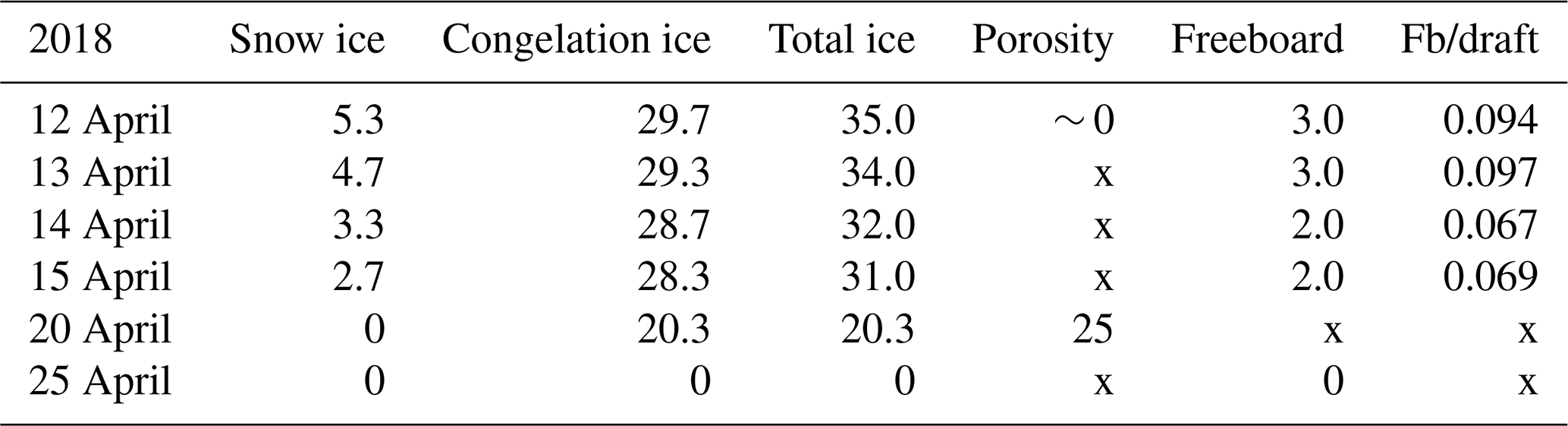
In 2018, the ice decay period began at the end of March, and the final breakup took place on 25 April. The thickness of ice was 42 cm on 30 March, and on 12 April it was 35 cm with 5.3 cm snow ice and 29.7 cm congelation ice (Table 1). Snow ice melted in less than 8 d, and congelation ice melted fast after 15 April. On 24 April, rain greatly accelerated the melting.
Table 1Thickness of ice layers and freeboard in the melting phase (cm) and porosity (%) in April 2018; also shown is the ratio of freeboard (Fb) to draft. Symbol x stands for no data.
3.1.2 Ice structure in the main experiment 2022
The ice decay period began on 25 March, and the final breakup took place after 42 d on 5 May (Table 2). The thickness of ice was 55 cm on 25 March, close to the long-term mean, with 33 cm congelation ice and 22 cm snow ice. During the decay period, the ice was melting at both boundaries and in the interior. At the end of April there was a slush layer between the surface ice layer and the congelation ice layer with soft places, so walking on the ice was not easy.
Table 2Thickness of ice layers and freeboard in the melting phase (cm) and porosity (%) in 2022; also shown is the ratio of freeboard (Fb) to draft. Symbol x stands for no data.
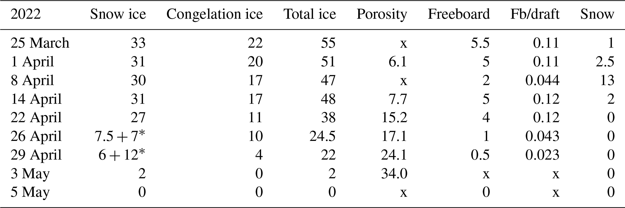
* Surface ice + slush layer.
Figure 2 shows drone orthophotos of the ice cover taken at an altitude of 100 m during the melting period. As reported by Ashton (1985) about melting lake ice in general, the ice cover of lake Pääjärvi looked grayish and patchy from above. Snowfall turned the ice white at the beginning of April, and as the air temperature increased, the new snow began to melt, creating a patchy surface. The positive albedo feedback of melting ice supports the persistence of surface patchiness.
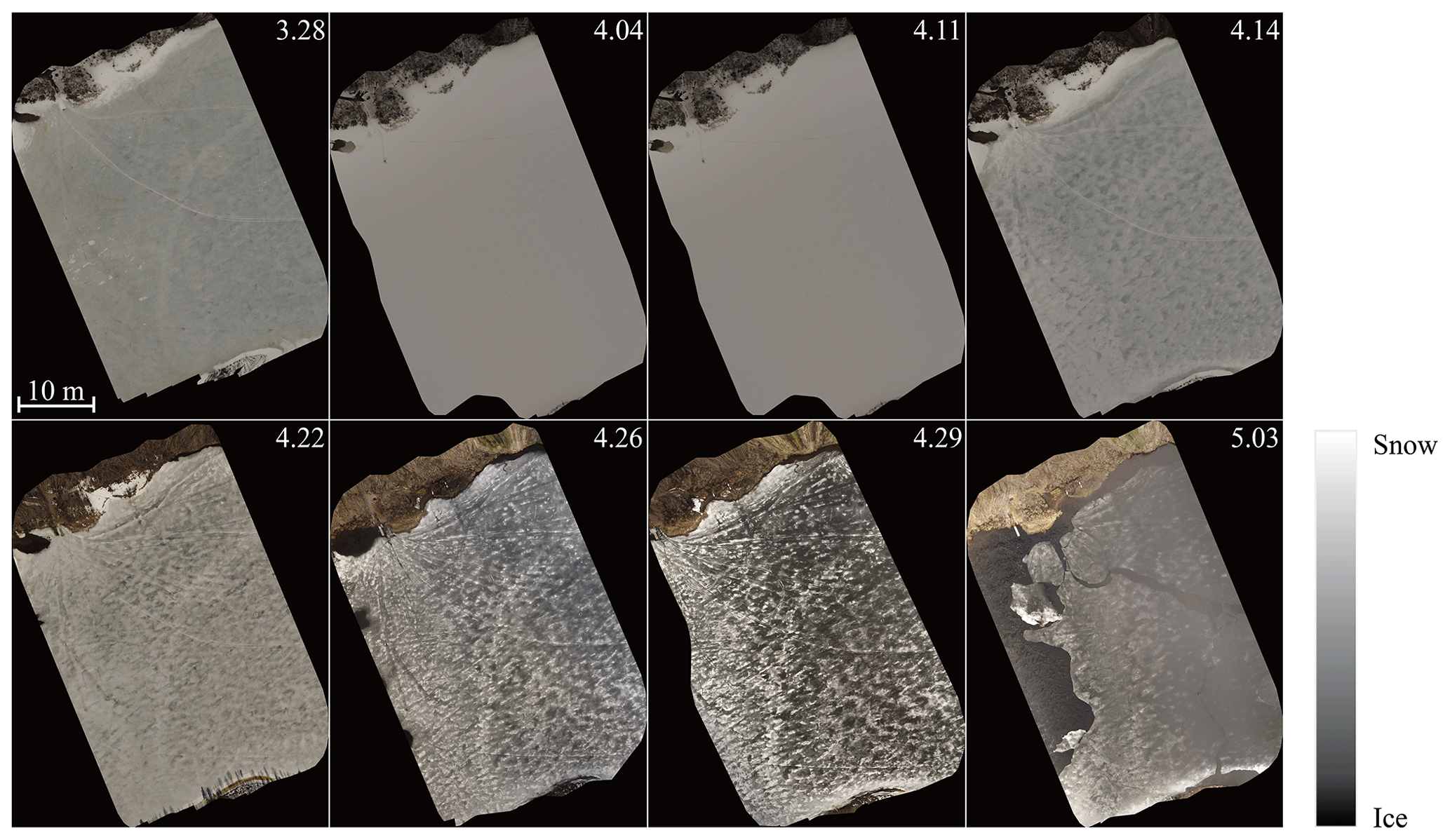
Figure 2Drone orthophotos of the ice cover in the melting period in 2022 (time given in m.dd format).
There were two principle vertical layers in the lake Pääjärvi ice cover (Fig. 3). The top layer was granular snow ice, with a grain size of 1–9 mm and blurred crystal boundaries, and the lower layer was clear columnar congelation ice with a grain size of 2–10 cm. When the ice melting progressed, the ice crystal structure data showed that the thickness of both snow ice and congelation ice decreased and that the porosity of ice increased.
The ice melted 4 cm during 25 May–1 April. On 1 April, the snow-ice part had two sublayers (Fig. 3). The top 27 cm sublayer had very irregular crystal structure with blurred crystal boundaries and grain size mainly within 1–2 mm. In the lower, 27–31 cm, layer the crystals were granular with clear boundaries, and the grain size was mainly 2–5 mm. It was judged that the upper sublayer had undergone a thawing and refreezing process. The columnar ice layer underneath was clear ice with grain size increasing with depth from 2 to 10 cm. The volume fraction of gas bubbles was 4 %–6 % in the snow-ice layer. They were cylindrical and spherical shaped with a maximum diameter of 4 mm. The corresponding fraction was 1 %–2 % in congelation ice, and the bubbles were spherical with a maximum diameter of 1 mm.
During 1–14 April, congelation ice melted by 3 cm, but snow-ice thickness was unchanged. According to the weather data, a snowfall began on 5 April, and then the air temperature rose, resulting in the formation of new snow ice through the melt–freeze cycle. Compared with 1 April, the ice crystal size had not changed, and the gas volume of snow ice was 5 %–7 %. After 14 April, the air temperature increased further, and the ice melted by 10 cm during 14–22 April. The horizontal and vertical sections showed strong melting at the grain boundaries in snow ice (Fig. 4a). The gas content increased in snow ice to 6 %–10 % and in congelation ice to 1 %–3 %. Also, the maximum diameter of gas bubbles increased to 5 mm in snow ice and 3 mm in congelation ice.
During 26–29 April, a slush layer appeared below a surface ice layer due to internal melting of ice (Fig. 4b). The columnar ice began to melt at crystal boundaries where gas inclusions appeared. On 29 April, the gas volume reached 5 % in the columnar layer, with the maximum bubble size equal to 5 mm. On 3 May, the columnar ice and slush layers had melted, and there was only 2 cm of snow ice left (Fig. 4c).
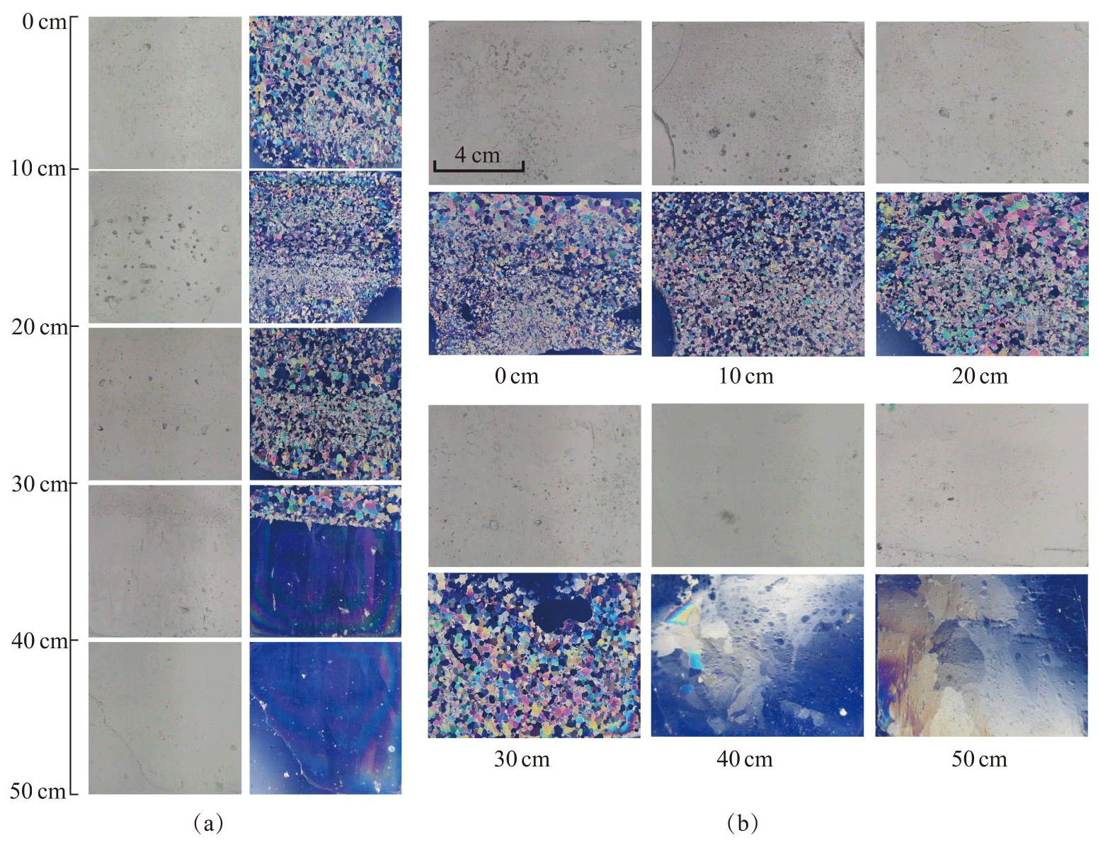
Figure 3Lake Pääjärvi ice crystal structure of 1 April. (a) Vertical profiles under normal light (left) and ice crystal structure under polarized light (right); (b) horizontal sections under normal light (top) and ice crystal structure under polarized light (bottom).
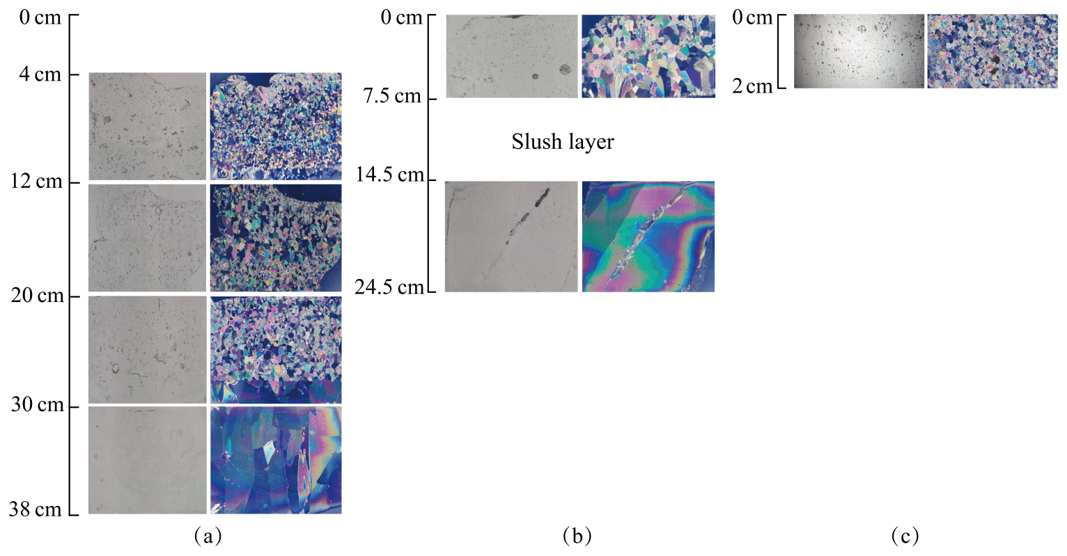
Figure 4Lake Pääjärvi ice crystal structure of 22 April, 26 April, and 3 May. (a) Vertical profiles under normal light (left) and ice crystal structure under polarized light (right) on 22 April; (b) vertical profiles under normal light (left) and ice crystal structure under polarized light (right) on 26 April; and (c) vertical profiles under normal light (left) and ice crystal structure under polarized light (right) on 3 May.
3.1.3 Ice melt rate
The ice sample data in Tables 1–2 were used to estimate the melting at the surface and bottom as well as in the ice interior. The melting rate increased toward the breakup date. In 2018 the ice cover was different from 2022 in that the ice was mostly (85 %) congelation ice (Table 1). During 12–20 April, the mean surface and bottom melting together was 1.84 cm d−1, and the mean internal melting was 0.86 cm d−1. During 12–15 April, the mean surface and bottom melting were 0.87 and 0.47 cm d−1, respectively. The ice was more transparent than in 2022, which allowed for more sunlight penetration through the ice. The bottom melting during 12–15 April corresponded to the heat flux:
where ρi is ice density, Lf is the latent heat of freezing, Δh is the change in ice thickness, and Δt=1 d.
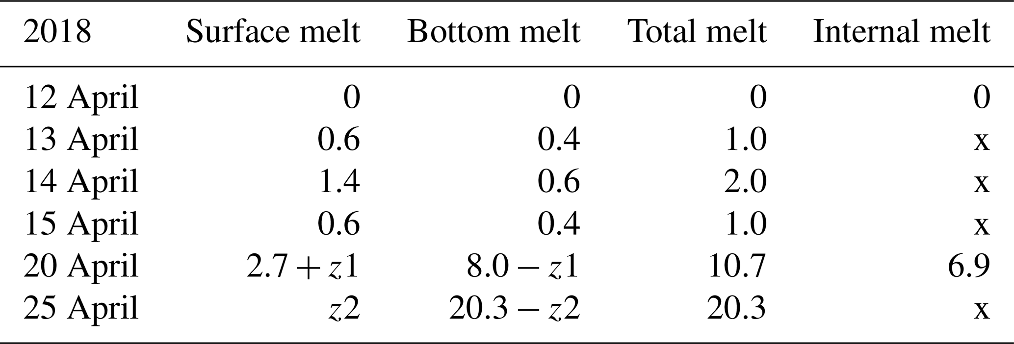
Table 3Ice melting in spring 2018 (cm). The numbers show the change from the row above to the present one. At the end, surface melting and bottom melting cannot be separated from the data as shown by z1 and z2. Symbol x is for no data.
In 2022 the mean rate was 1.31 cm d−1, and snow ice melted a little faster than congelation ice. The mean melt rates were 0.79 and 0.38 cm d−1, respectively. There was a minor new snow-ice formation on 14 April, and the last 2 cm thick piece was snow ice on 3 May. The mean melt rate at the bottom corresponds to a heat flux of 13 W m−2 from water to ice. This flux was larger than normally assumed (e.g., Yang et al., 2012). The mean internal melt rate was 0.18 cm d−1 equivalent ice thickness and was smaller than the surface and bottom melting, which was attributed to the low light transmittance of snow ice. In the last week of melting, the ice was highly porous and internal breakages occurred.
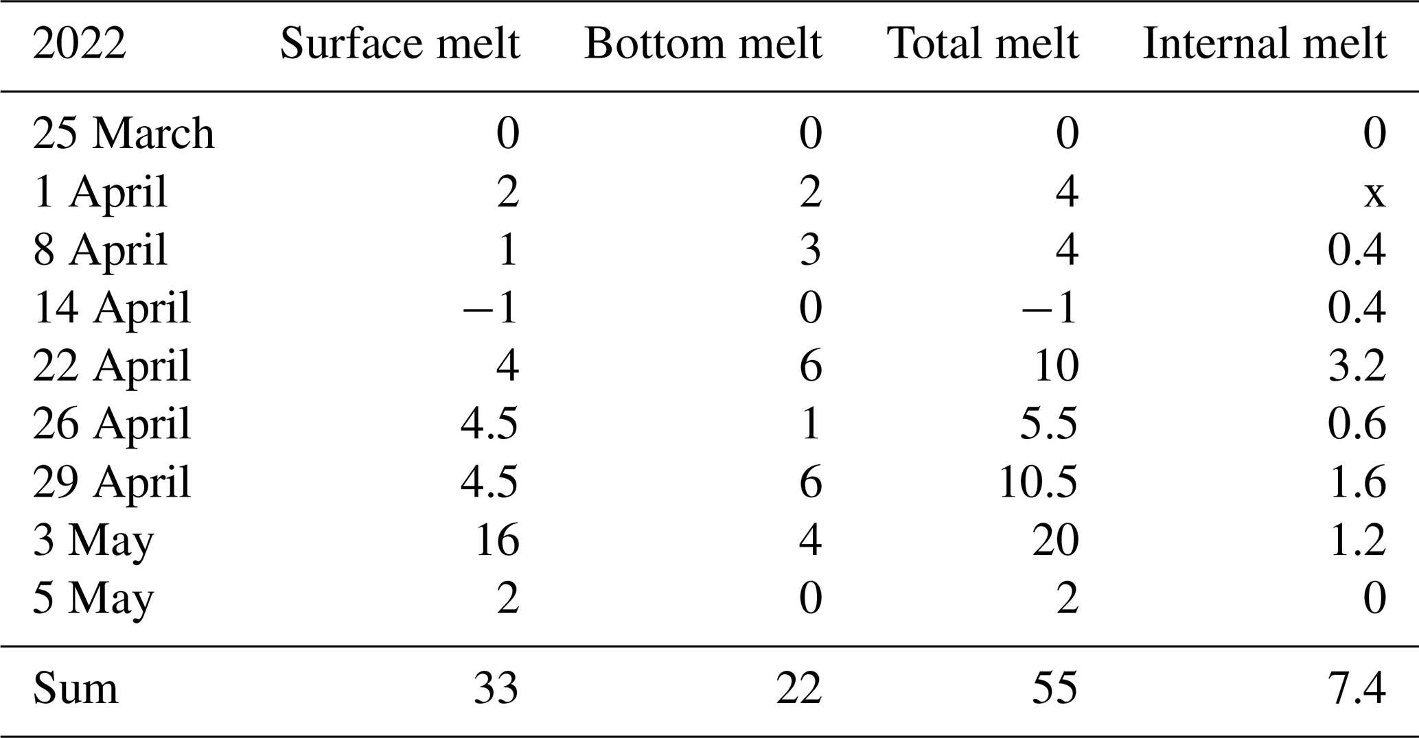
Table 4Ice melting in spring 2022 (cm). The numbers show the change from the row above to the present one. Symbol x is for no data.
3.2 Ice density
At the initial stage of melting, 1–14 April 2022, the estimated average densities of snow ice and congelation ice were 850 and 930 kg m−3, respectively. The congelation ice data are from the deep layers, and the apparently high density is likely due to liquid water in pores. The density profiles shifted toward a lower level with time, while the density always increased with depth (Fig. 5). On 22 April the snow-ice density was higher than on 14 April at great depth that can be due to meltwater accumulation in deep pores. Toward the ice breakup, the density decreased in snow ice to below 700 kg m−3 and in congelation ice to almost 700 kg m−3. The density data were used to estimate the porosity, which was found to increase from 6.1 % to 34 % during the melting period (Table 2).
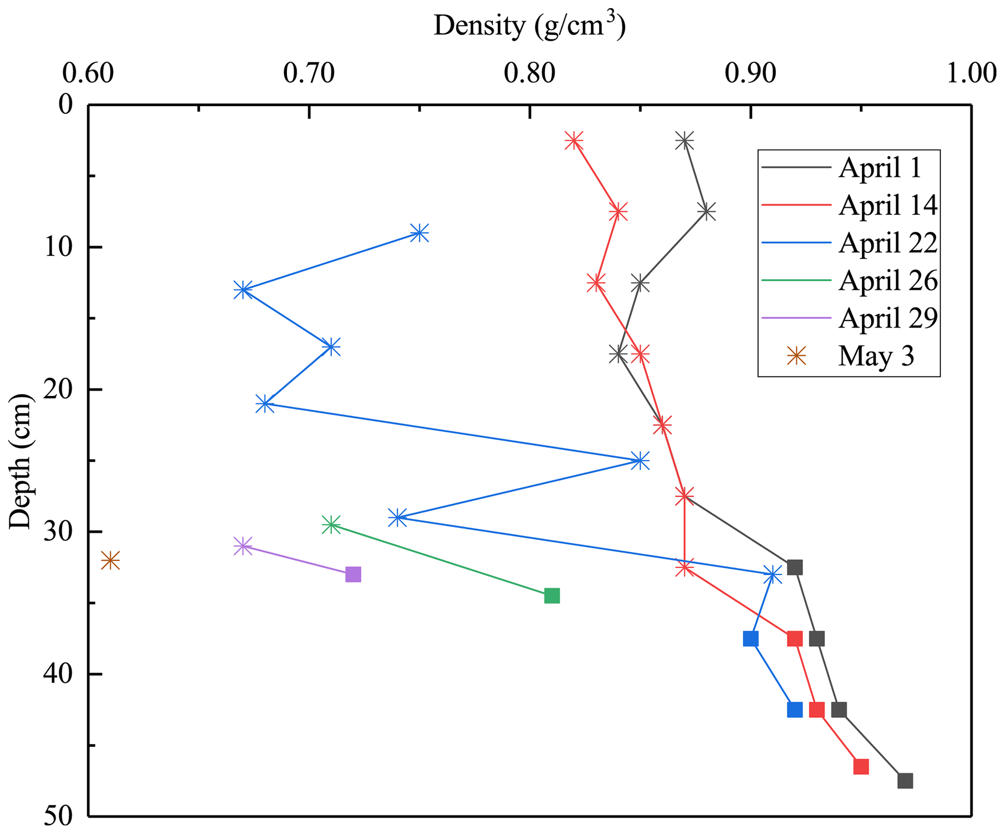
Figure 5Lake Pääjärvi ice density profiles in 2022 (asterisk stands for snow ice, square for congelation ice).
For bare ice, the freeboard-to-draft ratio is
where h is thickness and ρ is density, and the subscripts are w for water, d for draft, and f for freeboard. In winter, for kg m−3, this ratio is 0.10. It increases when the porosity decreases evenly, but it decreases if meltwater drainage from freeboard is trapped inside the draft to reduce the buoyancy. This is consistent with the present field observations.
3.3 Heat budget
We consider the volume of ice per unit area (V), expressed by the ice thickness (h) and porosity (ν) as . The external heat fluxes include the surface flux Q0, the heat flux from water to ice bottom Qw, and the absorption of solar radiation inside ice QA. It is assumed that in the melting stage the ice is isothermal with the temperature at the melting point. The heat fluxes are taken positive toward the ice, and for simplicity negative fluxes are ignored; that is, the model heat flux is . The surface and bottom fluxes reduce the thickness of ice, while the internal heating increases the porosity. Thus, we have the following (Leppäranta et al., 2019):
At the ice breaks due to its own weight, and the remaining ice pieces melt fast.
Here the surface heat flux is based on air temperature due to the lack of more complete atmospheric observations. The linearized approximate formula by Leppäranta (2015) is employed:
where k0 is independent of the surface temperature but depends on time, and k1∼15 W m−2 ∘C−1. In exact terms, k0 includes the radiation balance and latent heat flux at Ta=T0, and their correction for Ta≠T0 plus the sensible heat flux is included in k1. In lake Pääjärvi, k0 varies between −50 and 115 W m−2 in summer (Leppäranta and Wen, 2022). The second term in Eq. (4) represents the common degree-day model of ice melting, while the first term is geographic, representing the location (Leppäranta and Wen, 2022). The given value of k1 corresponds to the degree-day coefficient of 0.43 cm (∘C d)−1, which is close to the usual degree-day coefficient in hydrological forecasting (Leppäranta, 2015).
The internal melting and bottom melting depend on the solar radiation (see Leppäranta et al., 2019):
where α is albedo, γ≈0.5 represents the fraction of solar radiation that penetrates the surface (the light band), λ is the light attenuation coefficient, and c is the fraction of under-ice solar heating returning to ice bottom. Equation (5) gives the part of solar radiation used for internal melting, and the bottom melting in Eq. (6) consists of the background heat flux from the deep water (Qw0) and a part of the under-ice solar radiation.
The heat fluxes for ice melting in 2022 were estimated from Eqs. (4)–(6). The forcing was provided by the solar radiation data of FMI station Jokioinen and by the air temperature data of FMI station Lammi. It was assumed that the surface temperature was at the melting point. The incident solar radiation averaged to 126 W m−2 in the last week of March and 198 W m−2 in the first week of May, and the maximum daily average was 268 W m−2, on 25 April. The albedo was parameterized as α=0.7 for snow, 0.5 for dry ice, and 0.3 for wet ice, and λ=0.5 m−1 was fixed. The mean solar radiation and the mean air temperature were 184 W m−2 and 2.4 ∘C in April 2022, while the corresponding climatological values are 152 W m−2 and 3.5 ∘C.
The function k0 was estimated based on Leppäranta (2015): k0 increased from −35 W m−2 on 25 March to −1 W m−2 on 5 May. The total modeled surface melting became 36.6 cm, which is rather close to the observation (33 cm) obtained from the ice structure analysis (Table 3). The resulting mean absorption of solar radiation by ice was QA=5.6 W m−2, corresponding to the melt rate of 0.16 cm d−1, which is close to 0.18 cm d−1 obtained from the ice structure data. To evaluate the heat flux from the water, we took c=0.3 (Leppäranta et al., 2019), and then the contribution of solar radiation to the heat flux to ice bottom became 10.5 W m−2. The background term Qw0 is not known, but for molecular conduction the scale is W m−2, where kw=0.56 W m−1 ∘C−1 is thermal conductivity of water, and in general midwinter data suggest that Qw0<5 W m−2. With Qw0=1 W m−2, we have Qw=11.5 W m−2, and the corresponding melt rate at the ice bottom would be 0.33 cm d−1. This result is supported by the estimate Qw=13 W m−2 from the ice structure data in Sect. 3.1.
Ice melting obtained from the ice structure data is illustrated in Fig. 6. In 2022, the surface melting was greater than the bottom melting, while in 2018 it was the opposite. The main reason for this difference was in the ice stratification. In 2022, the snow-ice layer accounted for 60 % of the ice cover, while in 2018 the fraction was only 15 %. The melting rate was gradually increasing with the weather getting warmer and solar radiation increasing with time.
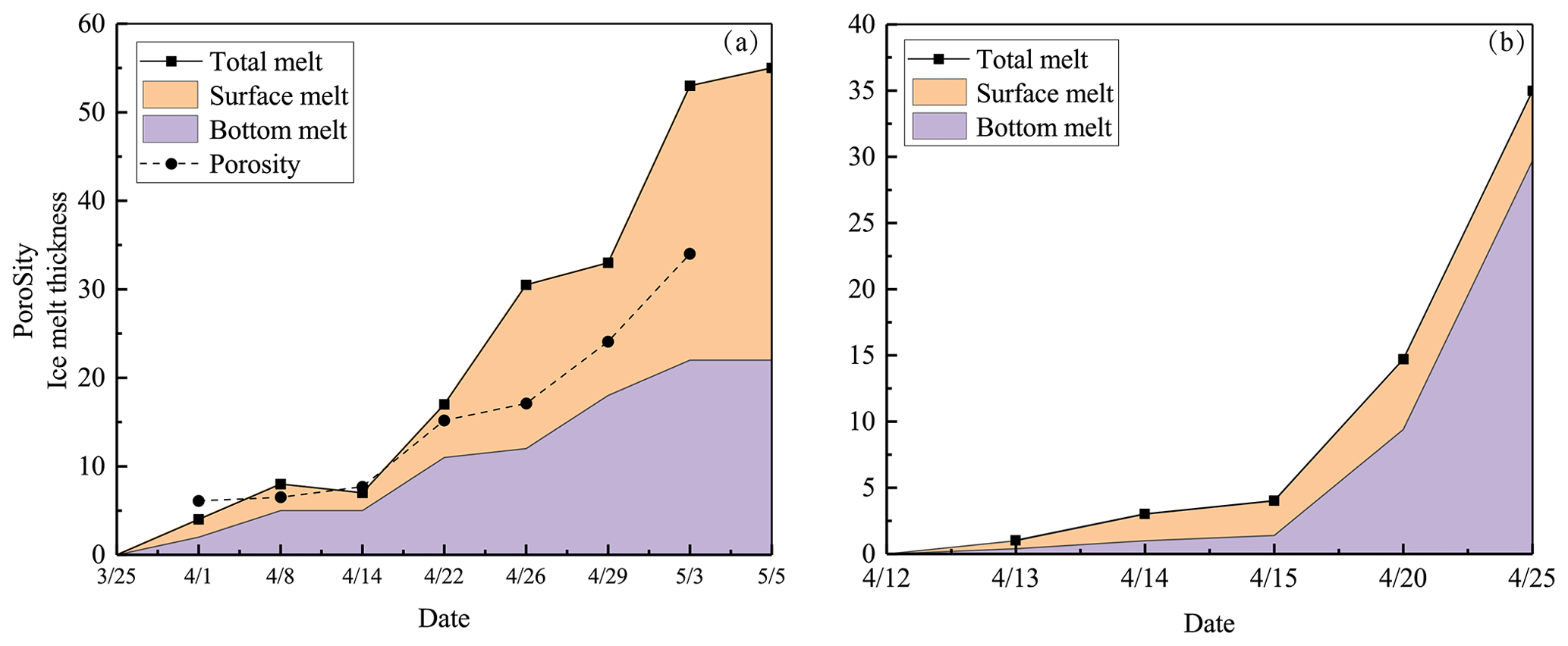
Figure 6Accumulated ice melting and porosity in 2022 (a) and 2018 (b) based on field data of ice structure. Porosity was not recorded in 2018.
3.4 Ice geochemistry
During the ice decay period, meltwater was mixed into the under-ice water layer that influenced the water geochemistry. In the present data, the meltwater had lower pH and EC than the lake water (Figs. 7–8). On 1 April 2022, the mean pH and EC of snow ice were 6.38 and 17.3 µS cm−1, respectively, and in congelation ice the corresponding values were 6.75 and 9.0 µS cm−1. Atmospheric deposition of acidic substances was judged as the background for the low pH of snow ice. Then pH and EC decreased. The vertical profiles of EC, pH, and Chl a show that EC was larger near the snow-ice surface than in congelation ice in the early melting stage, but the difference was no more obvious after 14 April. pH was always smaller in snow ice than in congelation ice. The content of Chl a was less than 0.6 µg L−1 with the maximum at the snow-ice–congelation-ice interface. In 2018, the limited data showed that EC was 6 µS cm−1 and pH was 6.35 in ice.
In lake water, the mean plus or minus standard deviation of pH and EC were 6.82 ± 0.09 and 92.5 ± 12.7 µS cm−1, respectively, in 2022. EC was smaller in ice by 1 order of magnitude than in water, on average EC(ice) = 0.12 ⋅ EC(water). EC was decreasing with time in water due to meltwater drainage from ice (Fig. 8). The changes in pH and EC had both signs, caused by flushing by meltwater and lake water. pH increased in the late melting period after the slush layer appeared, likely due to the increase in the photosynthesis-enhanced CO2 consumption. However, the inflow from brooks into the study bay could cause an opposite effect (Fig. 9). The inflow was weak until 21 April, but during 21–25 April it corresponded to 17 % of the water volume of the bay.

Figure 7EC, pH, and Chl a in ice meltwater and under-ice water at the study site in 2022 and 2018. (a) EC in ice meltwater and under-ice water at the study site in 2022; (b) pH in ice meltwater and under-ice water at the study site in 2022; (c) Chl a in ice meltwater and under-ice water at the study site in 2022; (d) EC and pH in ice meltwater and under-ice water at the study site in 2018.
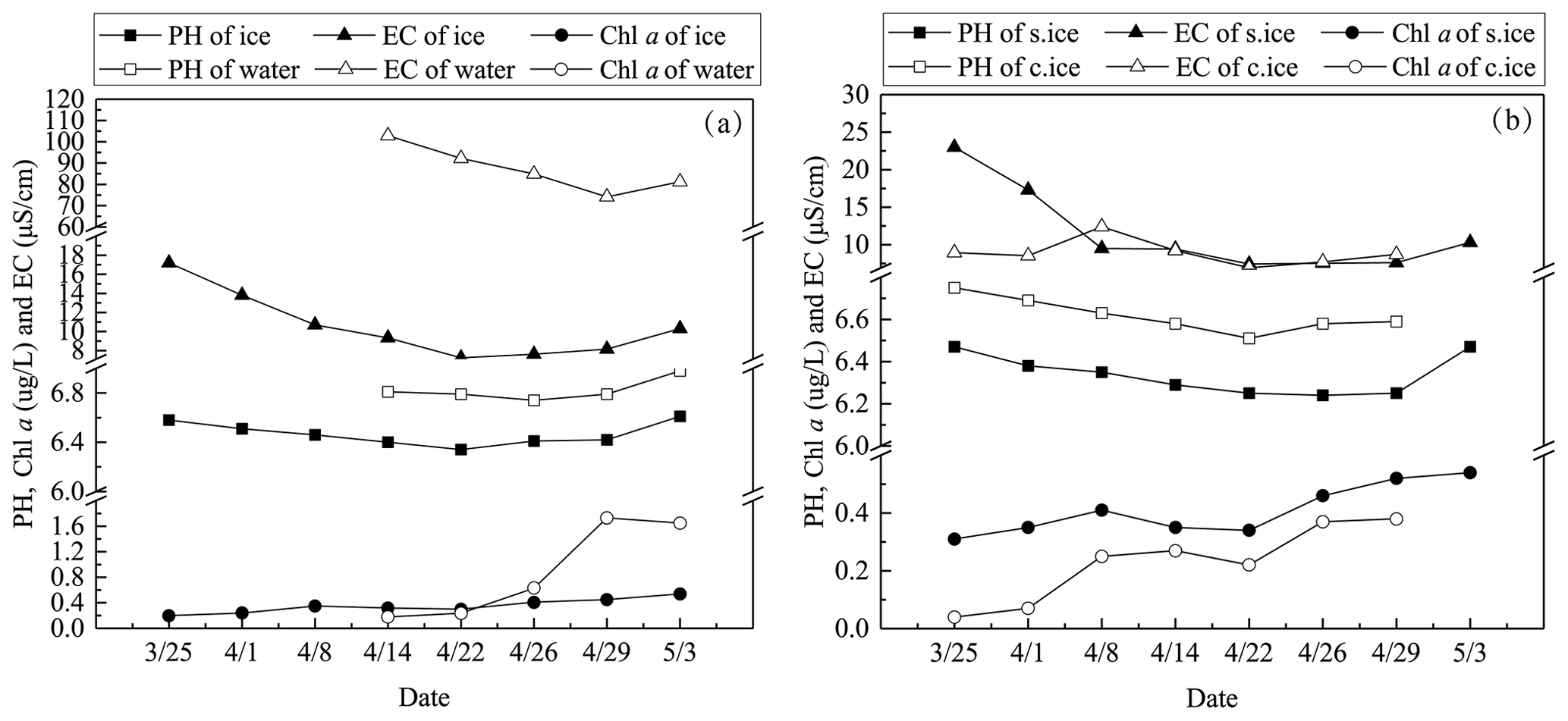
Figure 8The mean pH, EC, and Chl a in ice and lake water in 2022 (a) and the mean pH, EC, and Chl a in snow ice (s.ice) and congelation ice (c.ice) (b).
Algae can grow under ice and in slush layers in ice all winter at sufficient photon flux conditions. In springtime, algae growth occurs also in pores in ice-containing liquid water. Chl a content was similar in under-ice water and in ice until 26 April, but then it increased in water and became much higher than in ice at the time of ice breakup but still well below the first summer peak.
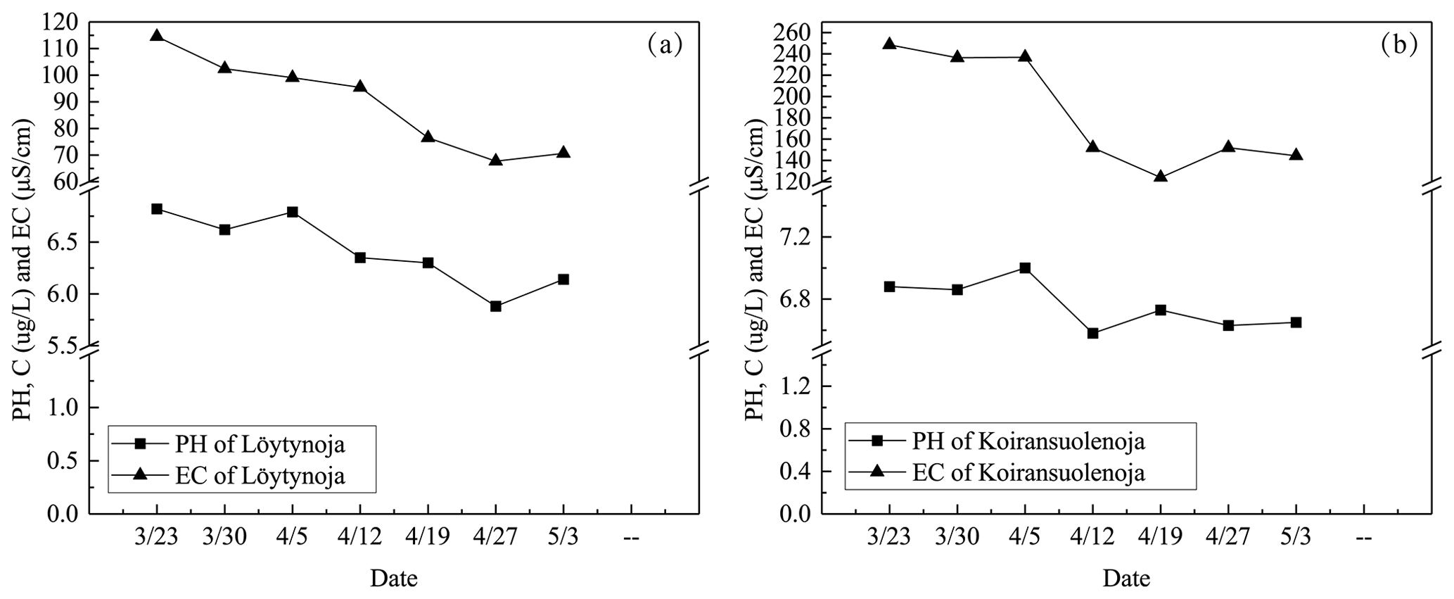
Figure 9pH and EC in two inflow brooks, Löytynoja (a) and Koiransuolenoja (b), to Pappilanlahti Bay.
4.1 Interannual variations of ice breakup date
Field data of lake ice are very important to examine and predict ice phenology, and the ice breakup date is an significant ice phenological parameter during the ice melting period (George, 2007; Williams et al., 2004; Stefan and Fang, 1997). Based on the ice breakup data from the Lammi Biological Station, we can see the interannual variations of ice breakup date in a boreal lake, Pääjärvi. The date of ice breakup is largely affected by solar radiation and the thickness and structure of ice and snow layers. Snow cover blocks the atmospheric and solar heat fluxes to the ice and prevents deterioration of the ice under snow. The first critical time in ice decay is the snow melting. Due to the positive albedo feedback and increasing solar radiation, it is difficult to pause melting. The melt rate of ice is 1–3 cm d−1, increasing with time.
The ice breakup date has become earlier in the last 50 years in lake Pääjärvi, but the interannual variability has been large (Fig. 10). During 1970–1990, the change was about 5 d per decade, which is more than can be explained by the regional warming, and the reason remains unclear. In general, in southern Finland the trend of the breakup date is 0.5–1 d earlier per decade as is typical in the global scale (Bernhardt et al., 2012; Magnuson et al., 2000). In northern Finland, lake Kilpisjärvi, the trend from 1964 to 2008 was 0.44 d over a decade toward earlier ice breakup (Lei et al., 2012). Earlier ice breakup has potentially widespread implications for 50 countries (Sharma et al., 2019). The loss of lake ice may lead to a reduction in the availability of fresh water due to increased evaporation, as well as to cultural and socioeconomic impacts to lake ice recreation, such as ice fishing and skating.
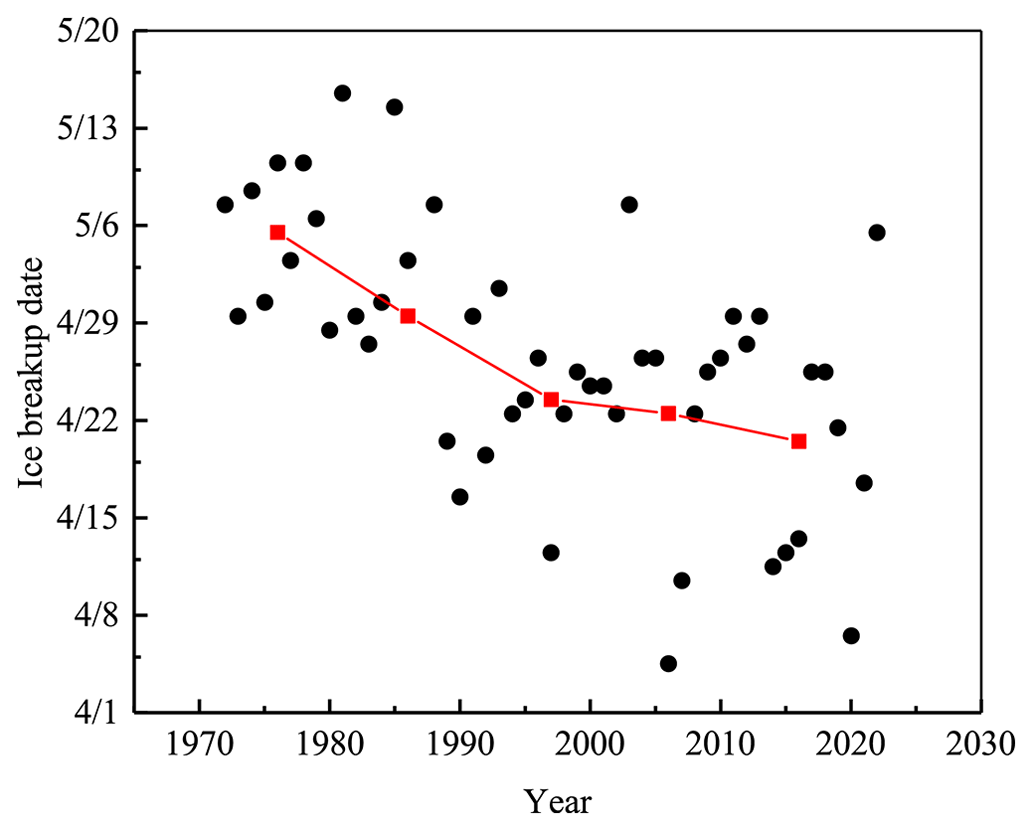
Figure 10The ice breakup date of lake Pääjärvi during 1970–2022. The black dots show the breakup date, and the red squares show the ice breakup date averaged every 10 years. Data source: Lammi Biological Station.
4.2 Comparisons of ice melting with other lakes
Melting of ice begins when the heat balance turns positive in spring and takes place at the surface, interior, and bottom, depending on the ice structure and fluxes. In 2022, the mean melting rate was 0.79 cm d−1 at the surface, 0.52 cm d−1 at the bottom, and 0.18 cm d−1 in the ice interior in lake Pääjärvi. In an Arctic tundra lake in northern Finland, lake Kilpisjärvi, the triplet (surface, bottom, and internal melting) was (2.9, 0.5, 1.0) cm d−1 in a warm spring 2013 and (0.8, 0.1, 1.0) cm d−1 in a normal spring 2014 (Leppäranta et al., 2019). In a boreal lake, lake Vendyurskoe, at 61–62∘ N, field investigations in two seasons showed the mean melt rates of 1.2 cm d−1 at the surface in both cases and 0.8 and 0.2 cm d−1 at the bottom (Leppäranta et al., 2010). The differences in the quality of melting are due to differences in the fractions of congelation ice and snow ice and weather conditions that determine the level of light transfer through ice and surface heat balance.
The porosity of ice needs to be estimated to examine the internal melting process. In the present work, the porosity was estimated from the measured ice density directly and from the absorbed solar radiation indirectly. The results were consistent with each other. Increasing porosity during the melting period changes the ice structure and decreases the strength of ice, and it finally leads to breakage with rapid final disappearance of ice. Here the breakage took place during 3–5 May when the porosity of the ice was 40 %–50 %. Leppäranta et al. (2019) used the solar radiation method to evaluate the porosity and found the same level at the breakage, supporting our result.
The heat flux from the lake waterbody to the bottom of ice has not been much studied (Shirasawa et al., 2006; Kirillin et al., 2012). A heat flux on the order of 1 W m−2 represents molecular conduction in the near-surface water layer and may be feasible in midwinter (e.g., Jakkila et al., 2009; Kirillin et al., 2012; Yang et al., 2012), but in spring, penetration of solar radiation to the waterbody gives a fractional return flux to the ice bottom. According to the present study, the heat flux from water to ice scales as 10 W m−2 in the melting period, and the more transparent ice allowed for more sunlight penetration and larger heat flux. Jakkila et al. (2009) reported the heat flux values in lake Pääjärvi as 12 W m−2 during the final stage of ice melting, which is very close to the present results, while Leppäranta et al. (2019) obtained 15–20 W m−2 in a warm spring but less than 5 W m−2 in a normal spring in a tundra lake. In the earlier literature, smaller values have been reported even at late stages of ice melting. For example, Bengtsson and Svensson (1996) obtained this heat flux ranging within 5–7 W m−2 during March–April in small Swedish lakes. Thus the picture of increasing bottom melting is clear, but the question anyway remains the most uncertain component of the heat budget of lake ice, and more research is needed (Kirillin et al., 2018).
The quality of ice decay is important for ice mechanics due to the loss of ice strength (Ashton, 1986; Leppäranta, 2015). There are two important consequences. First, the bearing capacity of ice (P) decreases. This quantity scales as M∝σfh2, where σf is the flexural strength, and during the melting period ice thickness and strength both decrease; thickness decreases due to melting at the boundaries, and strength decreases due to internal melting. The positive albedo feedback in the melting process produces a patchy ice cover, and together with the unpredictable bearing capacity the ice cover becomes a severe safety issue. Secondly, the two-dimensional yield strength of a lake ice cover scales as , where σc is the compressive strength of ice, and L is the lake size length scale. With decreased thickness and strength, wind stress may lead to ice breakage and ice movement on the shore, where damage can be caused to man-made structures since the ice strength is still finite.
4.3 Ice melting impact on geochemistry
Porous melting ice is permeable to water. Meltwater can flow down from the top, and lake water may penetrate to pores from below, which also influences the stratification of the under-ice water layer. Here the following basic geochemical properties were studied: pH, EC, and Chl a. They provide information about physical and chemical processes. The meltwater has lower EC than the lake water and, consequently, a lower density; therefore, a thin fresh surface layer may form just under the ice (Kirillin et al., 2012). The geochemistry also affects the physiological state of aquatic organisms, which will guide and predict the changes of biological structure in the water during the melting season.
The geochemistry under melting ice has been rarely reported. Lake Pääjärvi was studied for ice and water geochemistry in midwinter during 1996–1998 (Leppäranta et al., 2003). Their mean EC values in ice and water were close to our data, 16.5 and 108 µS cm−1, respectively, as compared with our 9.0 µS cm−1 for congelation ice, 17.3 µS cm−1 for snow ice, and 92.5 µS cm−1 for water; their mean EC in snow was 13 µS cm−1. In Leppäranta et al. (2003), pH was 6.7 for ice and 6.6 for water, but in our data pH was a little lower in snow ice and congelation ice than in lake water. Chl a was less than 0.5 µg L−1 in ice and between 0.2 and 1.7 µg L−1 in water, which is of the same order of magnitude reported by previous research (Leppäranta et al., 2003; Vehmaa and Salonen, 2009). Leppäranta et al. (2003) reported Chl a in ice also less than 0.5 µg L−1 in lake Pääjärvi but about 3 µg L−1 in a hypereutrophic lake 100 km from Pääjärvi. The present results are consistent with the previous studies; the small differences can be explained by the differences in the conditions of winters.
Ice season has a specific role in the local environment and human life, and it has an impact on the lake ecology far beyond the ice period. Research of lake ice has largely increased to evaluate the impact of the predicted climate change on the ice phenology and properties. During the melting period, it is difficult to do fieldwork due to the deterioration of the ice cover, and therefore only few data have been collected. In the present work, ice decay was monitored from the start to the final breakup, resulting in a full time series of the evolution of ice thickness, structure, and geochemical properties.
In 2022, the maximum thickness of ice was 55 cm with 60 % snow ice, and in 42 d the ice melted by 33 cm from the surface and 22 cm from the bottom, while the porosity increased from less than 5 % to 40 %–50 % at breakup. The comparison between ice structure and heat budget gave a good agreement in quantifying the deterioration of the ice cover. This result is promising when considering the possibility of detailed numerical modeling of ice deterioration. The largest uncertainty is in the bottom melting, where more research is needed on under-ice boundary layer dynamics. Solar radiation penetrating through ice adds a major contribution to the heat flux from water to ice, according to the present results on the order of 10 W m−2, which is significantly higher than usually assumed in lake ice modeling.
Ice and water pH and EC decreased during ice decay but experienced fluctuations due to flushing by meltwater and lake water. The mean EC of ice was 11.4 µS cm−1, which is equal to the fraction 0.12 of the lake water EC. The mean ice pH was 6.44, which is lower by 0.4 than in water. Chl a in ice increased to 0.6 µg L−1 in the later part of ice decay, with the maximum in the slush sublayer of snow ice. At the end of the decay, Chl a was 1.7 µg L−1 in water, which is still far from the first summer maximum.
The results are important for modeling the lake ice season and the annual cycle of lakes. Lake ice has an important role in the physical, chemical, and ecological cycle, and these cycles are sensitive to climate changes. For the ice melting season, detailed modeling of the ice strength as well as the consequent bearing capacity and ice forces has a major importance for the local societies in lake regions.
The ice sample, meteorological and hydrological data are available at the following link: https://doi.org/10.5281/zenodo.7903839 (Zhang et al., 2023).
YZ conceived the field and laboratory study in 2022 with ML, and MF and wrote the paper with contributions from JL and ZL. SS and JAK performed the study in 2018. All co-authors discussed the results and edited the manuscript.
The contact author has declared that none of the authors has any competing interests.
Publisher’s note: Copernicus Publications remains neutral with regard to jurisdictional claims in published maps and institutional affiliations.
We are grateful to the Lammi Biological Station and the Institute of Atmospheric and Earth Sciences, University of Helsinki, for providing logistical help and laboratories.
This work was supported by the National Key
Research and Development Program of China (grant no.
2019YFE0197600), the National Natural Science Foundation of
China (grant no. 52211530038), and the Academy of Finland
(grant nos. 350576 and 333889), as well as a personal grant to Yaodan Zhang by
the China Scholarship Council (CSC).
Open-access funding was provided by the Helsinki University Library.
This paper was edited by Bin Cheng and reviewed by two anonymous referees.
Arst, H., Erm, A., Herlevi, A., Kutser, T., Leppäranta, M., Reinart, A., and Virta, J.: Optical properties of boreal lake waters in Finland and Estonia, Boreal Environ. Res., 13, 133–158, 2008.
Arvola, L., Kankaala, P., Tulonen, T., and Ojala, A.: Effects of phosphorus and allochthonous humic matter enrichment on metabolic processes and community structure of plankton in a boreal lake (Lake Pääjärvi), Can. J. Fish. Aquat. Sci., 53, 1646–1662, https://doi.org/10.1139/f96-083, 1996.
Arvola, L., Salonen, K., Keskitalo, J., Tulonen, T., Järvinen, M., and Huotari, J.: Plankton metabolism and sedimentation in a small boreal lake – a long-term perspective, Boreal Environ. Res., 19, 83–96, 2014.
Ashton, G. D.: Deterioration of floating ice covers, J. Energy Resour. Technol.-Trans. ASME, 107, 177–182, https://doi.org/10.1115/1.3231173, 1985.
Ashton, G. D. (Ed.): River and lake ice engineering, Water Resources Publications, Littleton Colorado, ISBN 9780918334596, 1986.
Bengtsson, L. and Svensson, T.: Thermal regime of ice covered Swedish lakes, Hydrol. Res., 27, 39–56, 1996.
Benson, B. J., Magnuson, J. J., Jensen, O. P., Card, V. M., Hodgkins, G., Korhonen, J., Livingstone, D. M., Stewart, K. M., Weyhenmeyer, G. A., and Granin N. G.: Extreme events, trends, and variability in Northern Hemisphere lake-ice phenology (1855–2005), Climate Change, 112, 299–323, https://doi.org/10.1007/s10584-011-0212-8, 2012.
Bernhardt, J., Engelhardt, C., Kirillin, G., and Matschullat, J.: Lake ice phenology in Berlin–Brandenburg from 1947–2007: observations and model hindcasts, Climatic Change, 112, 791–817, https://doi.org/10.1007/s10584-011-0248-9, 2012.
Cavaliere, E. and Baulch, H. M.: Denitrification under lake ice, Biogeochemistry, 137, 285–295, https://doi.org/10.1007/s10533-018-0419-0, 2018.
Deng, Y., Li, Z., Li, Z., and Wang, J.: The experiment of fracture mechanics characteristics of Yellow River ice, Cold Reg. Sci. Tech., 168, 102896, https://doi.org/10.1016/j.coldregions.2019.102896, 2019.
Ellis, A. W. and Johnson, J. J.: Hydroclimatic analysis of snowfall trends associated with the North American Great Lakes, J. Hydrol., 5, 471–486, https://doi.org/10.1175/1525-7541(2004)005<0471:HAOSTA>2.0.CO;2, 2004.
Garcia, S. L., Szekely, A. J., Bergvall, C., Schattenhofer, M., and Peura, S.: Decreased snow cover stimulates under-ice primary producers but impairs methanotrophic capacity, mSphere, 4, 1–10, https://doi.org/10.1128/mSphere.00626-18, 2019.
George, G. D.: The impact of the North Atlantic Oscillation on the development of ice on Lake Windermere, Climatic Change 81, 455–468, https://doi.org/10.1007/s10584-006-9115-5, 2007.
Griffiths, K., Michelutti, N., Sugar, M., Douglas, M. S. V., and Smol, J. P.: Ice-cover is the principal driver of ecological change in high Arctic lakes and ponds, PLoS One, 12, 1–25, https://doi.org/10.1371/journal.pone.0172989, 2017.
Hampton, S. E., Galloway, A. W. E., et al.: Ecology under lake ice, Ecol. Lett., 20, 98–111, https://doi.org/10.1111/ele.12699, 2017.
Iliescu, D. and Baker, I.: The structure and mechanical properties of river and lake ice, Cold Reg. Sci. Tech., 48, 202–217, https://doi.org/10.1016/j.coldregions.2006.11.002, 2007.
Jakkila, J., Leppäranta, M., Kawamura, T., Shirasawa, K., and Salonen K.: Radiation transfer and heat budget during the melting season in Lake Pääjärvi, Aquat. Ecol., 43, 681–692, https://doi.org/10.1007/s10452-009-9275-2, 2009.
Karetnikov, S., Leppäranta, M., and Montonen, A.: Time series over 100 years of the ice season in Lake Ladoga, J. Gt. Lakes Res., 43, 979–988, https://doi.org/10.1016/j.jglr.2017.08.010, 2017.
Kirillin, G., Leppäranta, M., Terzhevik, A., Granin, N., Bernhardt, J., Engelhardt, C., Efremova, T., Golosov, S., Palshin, N., Sherstyankin, P., Zdorovennova, G., and Zdorovennov, R.: Physics of seasonally ice-covered lakes: a review, Aquat. Sci., 74, 659–682, https://doi.org/10.1007/s00027-012-0279-y, 2012.
Kirillin, G., Aslamov, I., Leppäranta, M., and Lindgren, E.: Turbulent mixing and heat fluxes under lake ice: the role of seiche oscillations, Hydrol. Earth Syst. Sci., 22, 6493–6504, https://doi.org/10.5194/hess-22-6493-2018, 2018.
Korhonen, J.: Long-term changes in lake ice cover in Finland, Hydrol. Res., 37, 347–363, https://doi.org/10.2166/nh.2006.019, 2006.
Langway, C. C.: Ice fabrics and the universal stage, Department of Defense, Department of the Army, Corps of Engineers, Snow Ice and Permafrost Research Establishment, 1959.
Lei, R., Leppäranta, M., Cheng, B., Heil, P., and Li, Z.: Changes in ice-season characteristics of a European Arctic lake from 1964 to 2008, Climatic Change, 115, 725–739, https://doi.org/10.1007/s10584-012-0489-2, 2012.
Leppäranta, M.: Interpretation of statistics of lake ice time series for climate variability, Hydrol. Res., 45, 673–683, https://doi.org/10.2166/nh.2013.246, 2014.
Leppäranta, M.: Freezing of lakes and the evolution of their ice cover, Springer, Berlin-Heidelberg, https://doi.org/10.1007/978-3-642-29081-7, 2015.
Leppäranta, M., and Kosloff, P.: The thickness and structure of Lake Pääjärvi ice, Geophysica, 36, 233–248, 2000.
Leppäranta, M. and Wen, L.: Ice phenology in Eurasian lakes over spatial location and altitude, Water, 14, 1037, https://doi.org/10.3390/w14071037, 2022.
Leppäranta, M., Tikkanen, M., and Virkanen J.: Observations of ice impurities in some Finnish lakes, Proc. Estonian Acad. Sci. Chem., 52, 59–75, 2003.
Leppäranta, M., Terzhevik, A., and Shirasawa, K.: Solar radiation and ice melting in Lake Vendyurskoe, Russian Karelia, Hydrol. Res., 41, 50–62, https://doi.org/10.2166/nh.2010.122, 2010.
Leppäranta, M., Lindgren, E., Wen, L., and Kirillin, G.: Ice cover decay and heat balance in Lake Kilpisjärvi in Arctic tundra, J. Limnol., 78, 163–175, https://doi.org/10.4081/jlimnol.2019.1879, 2019.
Li, Z., Jia, Q., Zhang, B., Leppäranta, M., Lu, P., Huang, W.: Influences of gas bubble and ice density on ice thickness measurement by GPR, Appl. Geophys., 7, 105–113, https://doi.org/10.1007/s11770-010-0234-4, 2010.
Magnuson, J., Robertson, D., Benson, B., Wynne, R., Livingstone, D., Arai, T., Assel, R., Barry, R., Card, V., Kuusisto, E., Granin, N., Prowse, T., Stewart, K., and Vuglinski, V.: Historical trends in lake and river ice cover in the Northern Hemisphere, Science, 289, 1743–1746, https://doi.org/10.1126/science.289.5485.1743, 2000.
Masterson D. M.: State of the art of ice bearing capacity and ice construction, Cold Reg. Sci. Tech., 58, 99–112, https://doi.org/10.1016/j.coldregions.2009.04.002, 2009.
Rouse, W. R., Binyamin, J., Blanken, P. D., Bussières, N., Duguay C. R., Oswald, C. J., Schertzer, W. M., and Spence, C.: The influence of lakes on the regional energy and water balance of the central Mackenzie River Basin, In: Cold Region Atmospheric and Hydrologic Studies: The Mackenzie GEWEX Experience, edited by: Woo, M. K., Springer, Berlin, 309–325, 2008a.
Rouse, W. R., Blanken, P. D., Duguay, C. R., Oswald, C. J., and Schertzer, W. M. : Climate-lake interactions. In: Cold Region Atmospheric and Hydrologic Studies: The Mackenzie GEWEX Experience, edited by: Woo, M. K., Springer, Berlin, 139–160, ISBN 9783540751366, 2008b.
Schroth, A. W., Giles, C. D., Isles, P. D. F., Xu, Y., Perzan, Z., and Druschel, G. K.: Dynamic coupling of iron, manganese, and phosphorus behavior in water and sediment of shallow ice-covered eutrophic lakes, Environ. Sci. Technol., 49, 9758–9767, https://doi.org/10.1021/acs.est.5b02057, 2015.
SFS 3021: Determination of pH-value of water, Finnish Standards Association (SFS), 1979.
SFS-EN 27888: Water quality. Determination of electrical conductivity, Finnish Standards Association (SFS), 1994.
Sharma, S., Blagrave, K., Magnuson, J. J., O'Reilly, C. M., Oliver, S.; Batt, R. D., Magee, M. R., Straile, D., Weyhenmeyer, G. A., and Winslow, L.: Widespread loss of lake ice around the Northern Hemisphere in a warming world, Nat. Clim. Change, 9, 227–231, https://doi.org/10.1038/s41558-018-0393-5, 2019.
Shirasawa, K., Leppäranta, M., Kawamura, T., Ishikawa, M., and Takatsuka, T.: Measurements and modelling of the water-ice heat flux in natural waters, Proceedings of the 18th IAHR International Symposium on Ice, Hokkaido University, Sapporo, Japan, 28 August–September 2006, 85–91, 2006.
Shoshany, Y., Prialnik, D., and Podolak, M.: Monte Carlo modeling of the thermal conductivity of porous cometary ice, Icarus, 157, 219–227, https://doi.org/10.1006/icar.2002.6815, 2002.
Stefan, H. G. and Fang, X.: Simulated climate change effects on ice and snow covers on lakes in a temperate region, Cold Reg. Sci. Tech., 25, 137–152, https://doi.org/10.1016/S0165-232X(96)00023-7, 1997.
Tan, Z., Yao, H., and Zhuang, Q.: A small temperate lake in the 21st century: Dynamics of water temperature, ice phenology, dissolved oxygen, and chlorophyll a, Water Resour. Res., 54, 4681–4699, https://doi.org/10.1029/2017WR022334, 2018.
Vehmaa, A. and Salonen, K.: Development of phytoplankton in Lake Pääjärvi (Finland) during under-ice convective mixing period, Aquat. Ecol., 43, 693–705, https://doi.org/10.1007/s10452-009-9273-4, 2009.
Wang, C., Shirasawa, K., Leppäranta, M., Ishikawa, M., Huttunen, O., and Takatsuka T.: Solar radiation and ice heat budget during winter 2002–2003 in Lake Pääjärvi, Finland, Verh. Internat. Verein Limnol., 29, 414–417, https://doi.org/10.1080/03680770.2005.11902045, 2005.
Warren, S. G.: Optical properties of snow, Rev. Geophys., 20, 67–89, https://doi.org/10.1029/RG020i001p00067, 1982.
Williams, G., Layman, K. L., and Stefan, H. G.: Dependence of lake ice covers on climatic, geographic and bathymetric variables, Cold Reg. Sci. Tech., 40, 145–164, https://doi.org/10.1016/j.coldregions.2004.06.010, 2004.
Yang, Y., Leppäranta, M., Cheng, B., and Li, Z.: Numerical modelling of snow and ice thicknesses in Lake Vanajavesi, Finland, TellusA, 64, 17202, https://doi.org/10.3402/tellusa.v64i0.17202, 2012.
Zhang, D., Fregona, M., Loehr, J., Ala-Könni, J., Song, S., Leppäranta, M., and Li, Z.: Data in “A field study on ice melting and breakup in a boreal lake, Pääjärvi, in Finland”, Version 1, Zenodo [data set], https://doi.org/10.5281/zenodo.7903839, 2023.