Chemical and visual characterisation of EGRIP glacial ice and cloudy bands within

Impurities in polar ice play a critical role in ice flow, deformation, and the integrity of the ice core record. Especially cloudy bands, visible layers with high impurity concentrations, are prominent features in ice from glacial periods. Their physical and chemical properties are poorly understood, highlighting the need to analyse them in more detail. We bridge the gap between decimetre and micrometre scales by combining the visual stratigraphy line scanner, fabric analyser, microstructure mapping, Raman spectroscopy, and laser ablation inductively coupled plasma mass spectrometry 2D impurity imaging. We classified approximately 1300 cloudy bands from glacial ice from the East Greenland Ice-core Project (EGRIP) ice core into seven different types. We determine the localisation and mineralogy of more than 1000 micro-inclusions at 13 depths. The majority of the minerals found are related to terrestrial dust, such as quartz, feldspar, mica, and hematite. We further found carbonaceous particles, dolomite, and gypsum in high abundance. Rutile, anatase, epidote, titanite, and grossular are infrequently observed. The 2D impurity imaging at 20 µm resolution revealed that cloudy bands are clearly distinguishable in the chemical data. Na, Mg, and Sr are mainly present at grain boundaries, whereas dust-related analytes, such as Al, Fe, and Ti, are located in the grain interior, forming clusters of insoluble impurities. We present novel vast micrometre-resolution insights into cloudy bands and describe the differences within and outside these bands. Combining the visual and chemical data results in new insights into the formation of different cloudy band types and could be the starting point for future in-depth studies on impurity signal integrity and internal deformation in deep polar ice cores.

1 Introduction

Deep ice cores from the polar regions revealed vast amounts of information regarding the climate of the past and processes taking place inside the ice. Pioneering deep ice cores were drilled almost 70 years ago at Camp Century, Greenland, or at Byrd Station, Antarctica. Over the last few decades, a variety of locations in Greenland and Antarctica were chosen for drilling operations (for an overview see Jouzel, 2013; Brook and Buizert, 2018). Considering different polar ice cores, most of the physical and chemical properties of ice and its impurities vary depending on several parameters that are different at each drilling site. Concurrently some features seem recurrent, such as the presence of the so-called “cloudy bands” in glacial ice.

Cloudy bands are horizontal, greyish-white stratigraphic layers with thicknesses between 1 mm and several centimetres (Fig. A1) (Gow and Williamson, 1976; Faria et al., 2010). They are characterised by a much finer ice grain size (∼1 mm) (in this study grain size refers to the ice crystal) than the surrounding ice and contain a very high concentration of micro-inclusions and other impurities (e.g. Ram and Koenig, 1997; Barnes et al., 2002; Svensson et al., 2005; Faria et al., 2010; Eichler et al., 2017). Gow and Williamson (1971, 1976) were among the first to describe cloudy bands in the Byrd ice core, where they observed dirt bands and the much more abundant cloudy bands. Dirt bands contained large particles, detectable by the eye, and were classified as volcanic ash bands. Cloudy bands, however, were not composed of visible debris but of a greyish-white appearance, hence the name (Gow and Williamson, 1971, 1976). The preferred crystal orientation within these bands is clustered about the vertical indicating strong horizontal shearing. Cloudy bands were thus associated with dust and deformation and provisionally interpreted as shear bands (Gow and Williamson, 1971, 1976).

Cloudy bands vary in thickness, brightness, and shape and are thus hard to constrain (Winstrup et al., 2012), but they have been discussed for a variety of reasons, ranging from climatic to deformation aspects (e.g. Svensson et al., 2005; Andersen et al., 2006; Faria et al., 2010; Winstrup et al., 2012; Westhoff et al., 2021). Svensson et al. (2005) show that, in most cases, the brightness variations of visual stratigraphy and cloudy bands match the seasonal cycles of tracers, especially of dust, derived by continuous flow analysis (CFA) (Fig. 5 in Svensson et al., 2005). Regularly appearing cloudy bands from visual stratigraphy were further used to date the Last Glacial Period (Andersen et al., 2006). Cloudy bands showing visible evidence of stratigraphic disturbances and even folding were declared the most significant optical stratigraphy feature helping to examine the integrity of deep ice cores, thus impacting scales larger than their size (Faria et al., 2010). The fine grains within cloudy bands could enable a more efficient diffusion due to the higher availability of impurity diffusion paths, such as veins along triple junctions and planes and interfaces along grain boundaries (Faria et al., 2010). Faria et al. (2010) concluded that cloudy bands are important for the disturbance of stratigraphic records on the micro-scale, indicating anomalies in the ice rheology. Impurity-enhanced ice flow in cloudy bands could impact ice core dating by enabling heterogeneous layer thinning (e.g. Paterson, 1991; Faria et al., 2006). Compression tests indicated that cloudy bands increase the flow enhancement factor in the flow law description by increasing the ratio of the observed strain rate to the strain rate produced on isotropic ice under the same stresses, and they thus affect the bulk deformation rate of ice softening it (Miyamoto et al., 1999). In these particular layers, microshear, i.e. the enhancement of dislocation creep by an accommodating mechanism involving grain boundary sliding (Kuiper et al., 2020) and microshear boundary formation (Bons and Jessell, 1999; Faria et al., 2006), could be a relevant microstrain mechanism. Developing a better understanding of the interplay between impurities and the microstructure in cloudy bands is thus necessary for a holistic understanding of deformation in polar ice (Stoll et al., 2021b).

Studies suggesting particulate matter as the main reason for the visibility of cloudy bands (Svensson et al., 2005; Faria et al., 2010) opposed speculations about their appearance due to micro-bubbles forming around impurities (Dahl-Jensen et al., 1997; Shimohara et al., 2003). Visual stratigraphy, dust, and Ca concentration correlate well in the NGRIP ice core (Svensson et al., 2005), similar to results of 90^∘ laser-light scattering and dust concentration in the GISP2 ice core (Ram and Koenig, 1997). Svensson et al. (2005) explain cloudy bands by the increased transport of mainly insoluble dust to the ice sheets. Each cloudy band thus represents a deposition event, i.e. precipitation or wind-driven sastrugi formation. Thin and bright bands could originate from low precipitation–dry deposition events or strong and early scavenging during snowfalls (Svensson et al., 2005).

High-resolution microstructural data are needed to truly investigate the origin, chemistry, and localisation of impurities in cloudy bands. Della Lunga et al. (2014) analysed a cloudy band with laser ablation inductively coupled plasma mass spectrometry (LA-ICP-MS), but the implementable resolution limited microstructural insights. Recent methodological progress now enables state-of-the-art LA-ICP-MS 2D chemical imaging of the total impurity content at the scale of a few tens of micrometres (Bohleber et al., 2020, 2021), in particular when focusing also on dust-related elemental species (Bohleber et al., 2023). Furthermore, cryo-Raman spectroscopy (e.g. Ohno et al., 2005; Sakurai et al., 2009) coupled with microstructure mapping (Eichler et al., 2017, 2019; Stoll et al., 2021a, 2022) was established as a powerful tool to localise and identify solid micro-inclusions in the microstructure of ice.

This study aims to investigate glacial ice from the East Greenland Ice-core Project (EGRIP) ice core and cloudy bands within, applying Raman spectroscopy and microstructure mapping complemented by visual stratigraphy, grain size, and LA-ICP-MS 2D imaging analyses. These methods cover several spatial scales, ranging from decimetres to micrometres, enabling a holistic analysis of the EGRIP ice core, whose visual stratigraphy was measured continuously (Westhoff et al., 2021, 2022) and whose shallower part was investigated regarding its microstructure, and the distribution, quantity, and quality of impurities (Stoll et al., 2021a, 2022; Bohleber et al., 2023). In the upper 1340 m of the core, i.e. the Holocene, Younger Dryas, and the Bølling–Allerød, micro-inclusions are mainly in the grain interior and show a strong heterogeneity in distribution. Inclusions are mainly gypsum, quartz, feldspar, and mica, and mineral diversity decreases slightly with depth, while the upper 900 m is characterised by various sulfate minerals, such as Mg, Na, and K sulfates or bloedite. In this study, we analyse the mean grain size evolution of the glacial and classify different cloudy bands and their abundance using visual stratigraphy. We explore different cloudy band types and discuss possible origins. To increase our understanding of impurity-related processes in ice, we locate and identify the mineralogy of more than 1000 micro-inclusions using Raman spectroscopy, focusing on cloudy bands. To explore future possibilities, we conduct LA-ICP-MS 2D chemical imaging on a subset of these previously analysed samples to obtain spatial information on the major soluble and insoluble elements, such as Na, Mg, Sr, Al, Ti, and Fe. Together, this results in a detailed study of the chemical and visual properties of EGRIP glacial ice with an emphasis on cloudy bands.

2 Methods

2.1 The East Greenland Ice-core Project

EGRIP is a deep ice core drilling project located on the Northeast Greenland Ice Stream (NEGIS), the largest ice stream in Greenland (Fahnestock et al., 1993; Vallelonga et al., 2014). The drill site is located at 75^∘37.820^∘ N and 35^∘59.556^∘ W, 2704 m a.s.l., 440 km to the southeast of the NEEM site. The ice flow velocity at the drill site is ∼55 m yr⁻¹ (Hvidberg et al., 2020). To date, 2418 m of ice has been drilled and partly processed, with ∼250 m remaining to bedrock.

2.2 Grain size measurements

Ice grain size was measured at EGRIP on discrete samples every 5–15 m of depth. The 55 cm samples were cut into six samples (parallel to the core axis) with dimensions of $\sim \mathrm{90}\times \mathrm{70}\times \mathrm{0.3}$ mm. Samples were polished and measured with an automated G50 fabric analyser (Russell Head type Wilson et al., 2003). Details about the procedure and data processing are found in Stoll et al. (2021a).

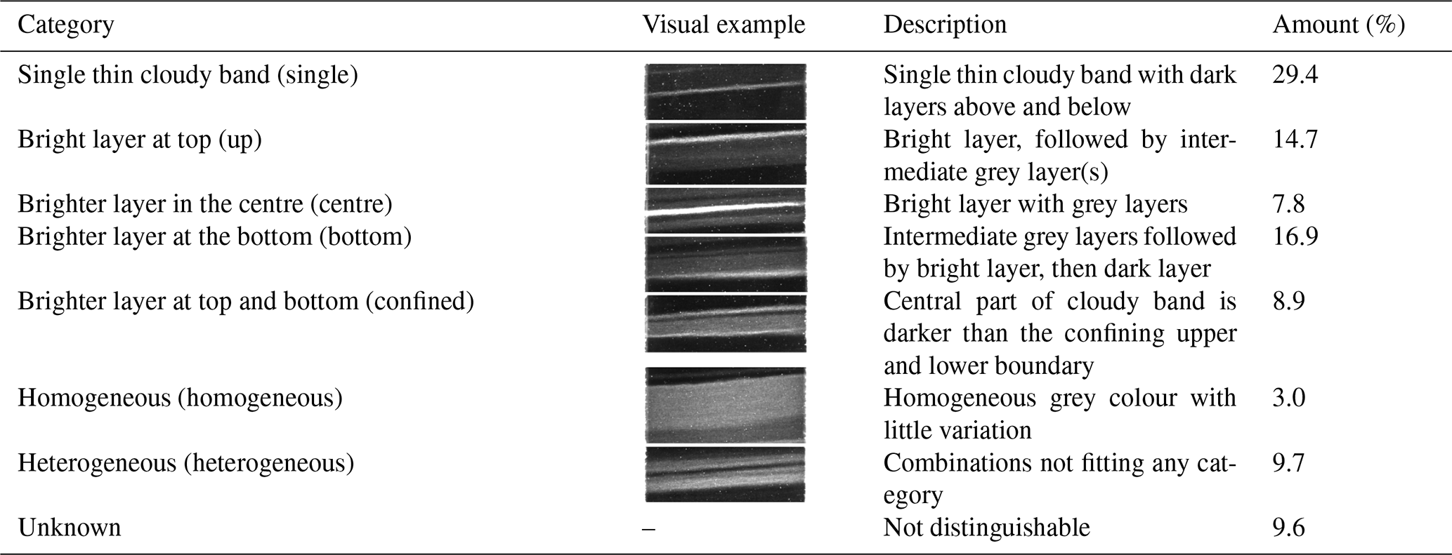
Table 1 Different cloudy band types in EGRIP Last Glacial Period ice. Image width is 7 cm.

2.3 Visual stratigraphy

Visual stratigraphy measurements, i.e. line scans, were conducted in the EGRIP trench shortly after the core retrieval to avoid signal alteration (Svensson et al., 2005), with some buffer time in between to account for differences in atmospheric pressure. Brittle zone ice was measured a year after retrieval to lower the risk of ice breaking during processing.

Processed line scan data are available from 13.75 to 2120 m depth (Weikusat et al., 2020). The instrument used was a Schäfter+Kirchhoff GmbH line scanner, developed in cooperation with the Alfred Wegener Institute Helmholtz Centre for Polar and Marine Research (AWI) and the University of Copenhagen (details in Svensson et al., 2005; Faria et al., 2018; Westhoff et al., 2022). Slabs of ice were polished from both sides and illuminated from below (“dark field” imaging). The light is scattered by solid impurities, fractures, and bubbles and directed back into the camera making them visible. In glacials, the main scattering objects are cloudy bands and fractures.

2.3.1 Cloudy band types

To compare cloudy bands throughout the ice core, a consistent camera setting is of uttermost importance. Below a depth of 1375 m (bag 2500, 14.6 ka b2k Gerber et al., 2021) constant settings were used. We do not investigate cloudy bands from the Holocene (Westhoff et al., 2022). We exclude 55 cm ice cores from the analysis where most cloudy bands show deformation features to eliminate a complication factor. Yet some samples can contain single cloudy bands showing signs of deformation or belonging to more than one group. To also account for these bands, without being able to group them into a certain category, we group them as “unknown” (examples in Fig. A2).

Andersen et al. (2006) and Winstrup et al. (2012) showed that cloudy bands appear in an annual cyclicity and that a single cloudy band, i.e. a stack of bright layers, is situated between two dark layers. We thus define a cloudy band by an upper and lower dark layer boundary, i.e. all bright layers between two dark layers are defined as one cloudy band. We identified seven different types of cloudy bands, designed to be specific identifiers, i.e. mutually exclusive classes, depending on where the brightest layer of one cloudy band is situated (Table 1). We find thin single bright layers (single), bright layers with an even brighter layer at the top (up), in the middle (centre), or in the bottom (bottom). We identify two bright layers confining a less bright layer at the top and bottom (confined), a thick bright layer with very few brightness variations (homogeneous), or a mix of the above, mostly with thin alternating layers (heterogeneous). Some layers cannot be clearly grouped (unknown), either because the images are too dark, the layers too thin, or features are folded. Our cloudy band types are also visible in the NEEM and NGRIP ice cores and are thus probably representative of Greenland.

2.3.2 Greyscale

The greyscale analysis investigates brightness variations caused by the scattering of light by features in the ice core. Variations occur on the millimetre to centimetre scale (cloudy bands) and the metre scale (stadials–interstadials). For the depth of investigation, we analyse the brightness derived from the pixel values of the line scan greyscale images. Values are between 0 and 255, providing 256 possibilities. One centimetre in length is equivalent to 186 pixels in the image files, generating a high-resolution depth series of brightness variations.

2.4 Raman spectroscopy

The remaining pieces of the fabric analyser samples were cut into cubes of ca. 2×2 cm (Table 2) and polished from two sides with a microtome to enable successful microstructure mapping (Stoll et al., 2021a) and Raman spectroscopy analyses (Stoll et al., 2022).

Raman spectroscopy measurements were conducted in a cold lab (−17 ^∘C) at AWI in Bremerhaven, Germany. The spectrometer, excitation laser, and control unit are located at room temperature close to the cold lab, which contains the microscope unit. A 100 µm fibre was used for good signal intensity and confocality. We used a WITec alpha300 M+ combined with a Nd:YAG laser (λ=532 nm) and a ultra-high throughput spectrometer (UHTS) 300 spectrometer with a 600 grooves per millimetre grating. The pixel resolution is <3 cm⁻¹ and the spectral range is >3700 cm⁻¹. A Hg/Ar spectral calibration lamp was used to calibrate the system. Spectra were background corrected and identified using the RRUFF database (Lafuente et al., 2015) and reference spectra (e.g. Eichler et al., 2019; Stoll et al., 2022).

2.5 Laser ablation inductively coupled plasma mass spectrometry 2D impurity imaging

Following Raman spectroscopy analysis at AWI, the samples were transported via a commercial freezer transport to Ca'Foscari University of Venice. Micrometre-resolution LA-ICP-MS 2D imaging was performed with a set-up comprised of an Analyte Excite ArF excimer 193 nm laser (Teledyne CETAC Photon Machines) with a HelEx II two-volume ablation chamber. The ablated material is transported to an iCAP-RQ quadrupole ICP-MS (Thermo Scientific) via a rapid aerosol transfer line. Samples surfaces are cleaned and polished with ceramic ZrO₂ blades (American Cutting Edge, USA) before placing them on a cryogenic sample holder. Before each measurement, 1–2 pre-ablation runs are conducted with an 80×80 µm spot to clean the surface of interest before the analysis. Before and after each measurement one scan line on a standard (NIST glass SRM 612) is acquired to monitor potential instrumental drifts. We used laser spot sizes of 35 and 20 µm on the following samples analysed earlier with Raman spectroscopy: S2, S4, S7, S8, S10, S11, and S12 (Table 2). We followed a newly refined multi-element imaging method including dust-related elements as described in Bohleber et al. (2023). In order to consider species with mostly soluble and mostly insoluble behaviour, we measured the following analytes: ²³Na, ²⁴Mg, ²⁷Al, ⁴⁸Ti, ⁵⁶Fe and ⁸⁸Sr.

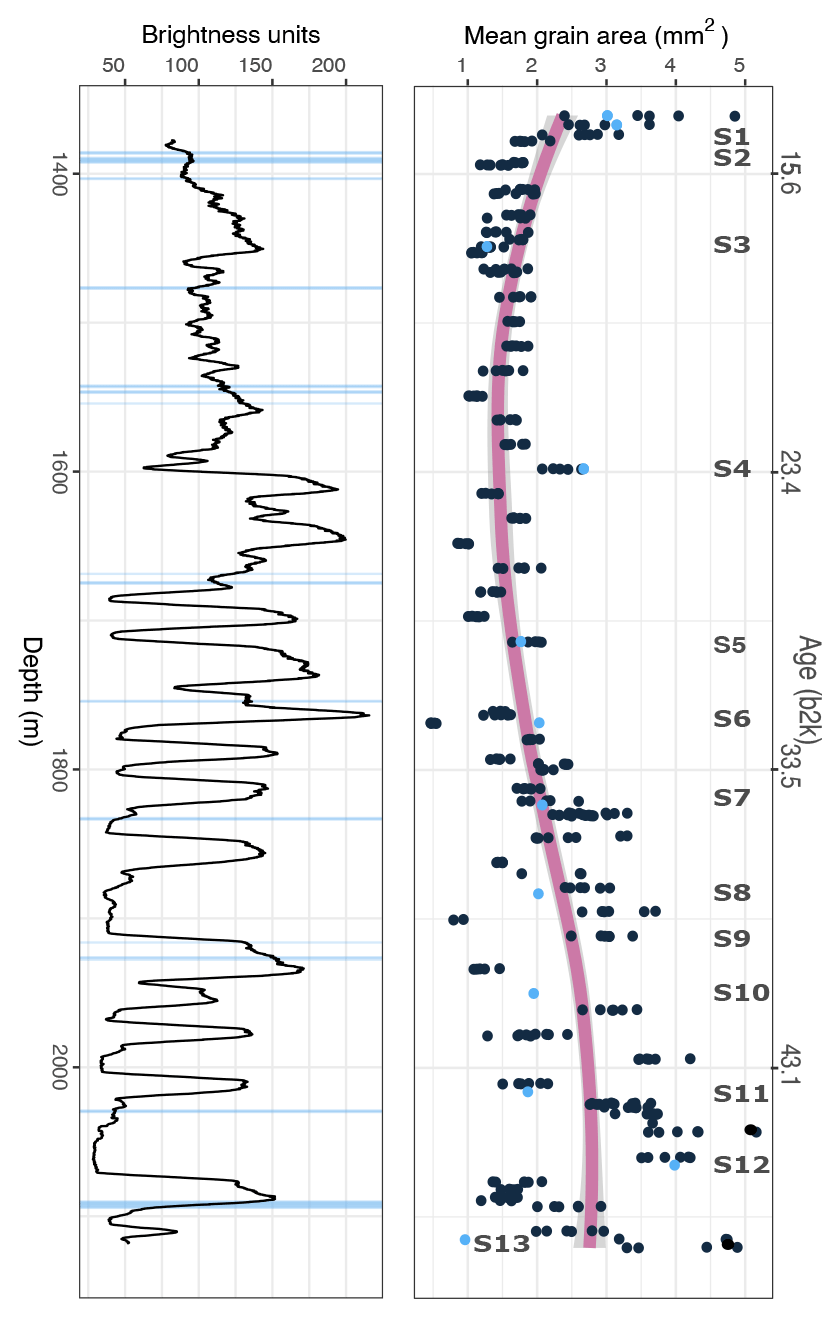
Figure 1 Greyscale with depth smoothed with a 5 m running mean. Horizontal light blue lines indicate 55 cm long ice cores analysed for cloudy band types. Mean grain areas use 9 cm samples from the G50 fabric analyser. Samples analysed with Raman spectroscopy are indicated in blue (S1–S13) (exact depths in Table 2); data for S9 are not available. The violet line is a locally weighted regression with a smoothing parameter of 0.3. Age is from Gerber et al. (2021).

3 Results

3.1 Grain size

Mean grain size decreases from 3.6 mm² at 1340 m depth to 1–2 mm² by 1800 m (except 2–2.7 mm² at 1600 m depth) (Fig. 1). The mean grain size is at its minimum between 1500 and 1700 m, correlating with the Last Glacial Maximum (LGM). Below this point, values increase and spread with depth and are between 0.8 and 5.2 mm². Analysed thin sections contain between 471 and 4550 grains.

3.2 Visual stratigraphy – greyscale and cloudy band types

The greyscale analysis (Fig. 1), i.e. the brightness variations of line scan images, is a proxy for the solid particle concentration (Svensson et al., 2005) and shows fluctuations following the glacial stadials and interstadials. The data enable classifying the brightness of cloudy bands: <100 is dark, 100 to 150 is medium dark, around 150 is medium, 150 to 200 is medium bright, and 200 to 255 is bright.

We classified 1267 cloudy bands into seven types (Fig. 2). The type single is the most abundant one making up 29 % of all cases (Table 1). The types up and bottom, i.e. a bright layer at the top or bottom of a homogeneous layer, add up to 15 % and 17 %, respectively. The types confined (9 %), heterogeneous (10 %), and centre (8 %) make up another third of all cloudy band types. Rarest is the thick homogeneous (3 %) type. Almost 10 % could not be distinguished clearly (unknown).

Throughout the analysed depth, the relative distribution of cloudy bands varies per 55 cm section, especially for single, homogeneous and heterogeneous types (Fig. 2a). Single cloudy bands occur more often with depth and range from 5 % to above 50 % of identified types per 55 cm ice core. The types up, centre, and bottom are fairly constant. The type unknown occurs more frequently in deeper ice (Fig. 2a) as layers thin and categorisation becomes more difficult. Furthermore, the darkness of the image plays a role. For consistency, throughout the glacial the brightness is kept constant for all images, thus making our analysis more favourable for stadials, i.e. cold periods with a higher dust concentration, within the Last Glacial Period.

We identified 989 and 278 cloudy bands in Greenland stadials and interstadials, respectively. Single dominates both period types (if identifiable) with a similar relative abundance (Fig. 2b). Especially bottom, heterogeneous, and confined cloudy bands are more common in stadial ice. However, 27.3 % of cloudy bands in interstadials could not be identified clearly (type unknown) compared to 4.6 % in stadials.

Table 2 Samples analysed with Raman spectroscopy and LA-ICP-MS (×). The depth refers to the middle of the area analysed with Raman spectroscopy.

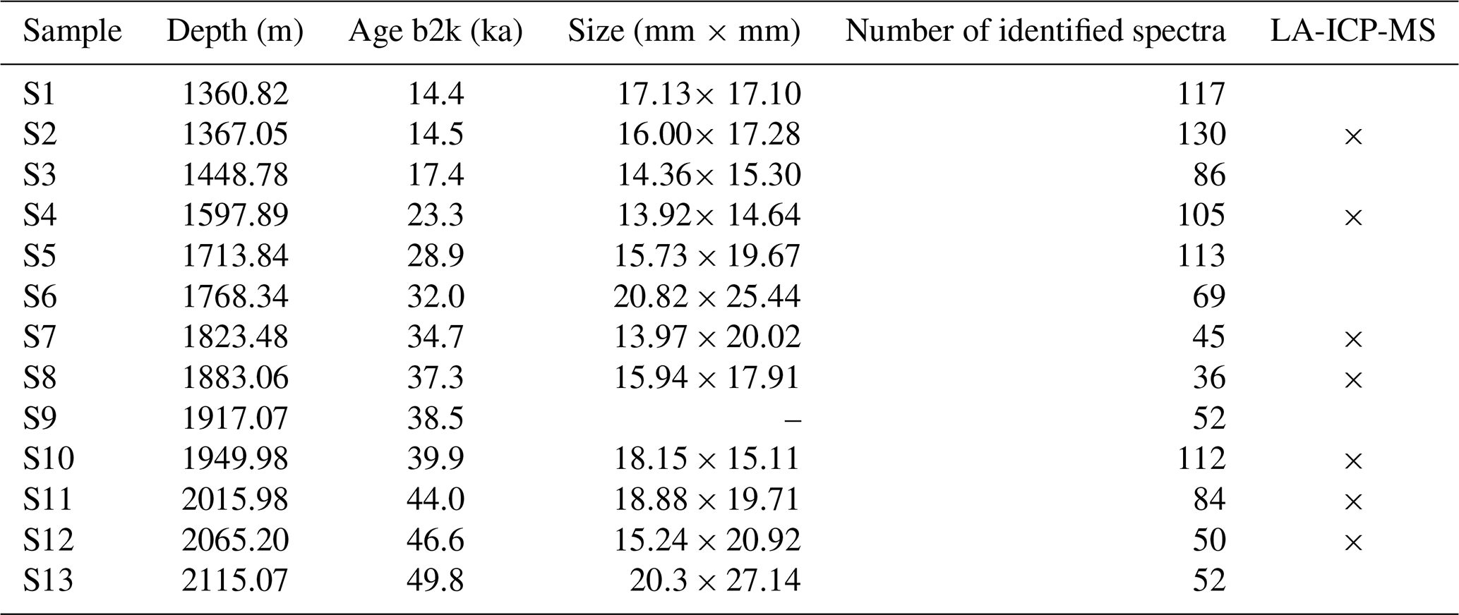
b2k: before 2000 CE (Gerber et al., 2021). In S9, a specific cloudy band was analysed, but the sample was not cut into specific dimensions.

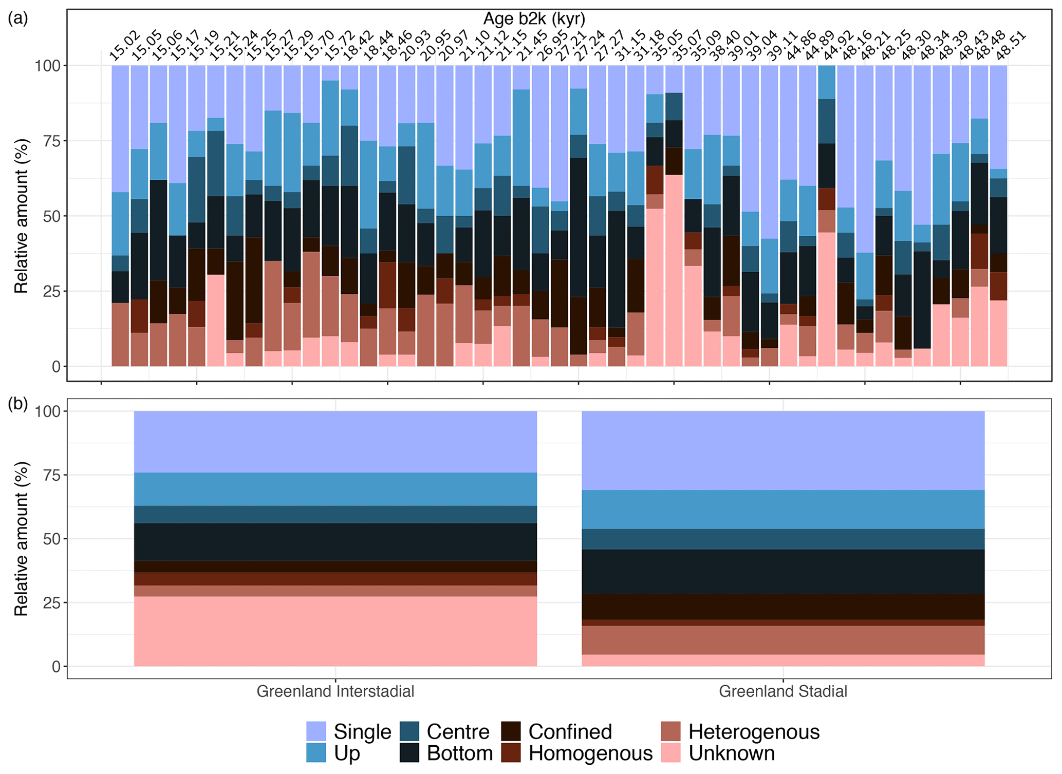
Figure 2 Different cloudy band types in EGRIP glacial ice. (a) Cloudy band types per 55 cm ice cores (depths are shown in Fig. 1) containing identifiable cloudy bands between 15.02 and 48.51 ka before 2000 CE (Gerber et al., 2021). The different types seen in the visual stratigraphy data are described in Table 1. (b) Relative amounts of all classified cloudy band types in our samples found in either Greenland interstadials or stadials (after Rasmussen et al., 2014).

3.3 Raman spectroscopy

3.3.1 Identified minerals

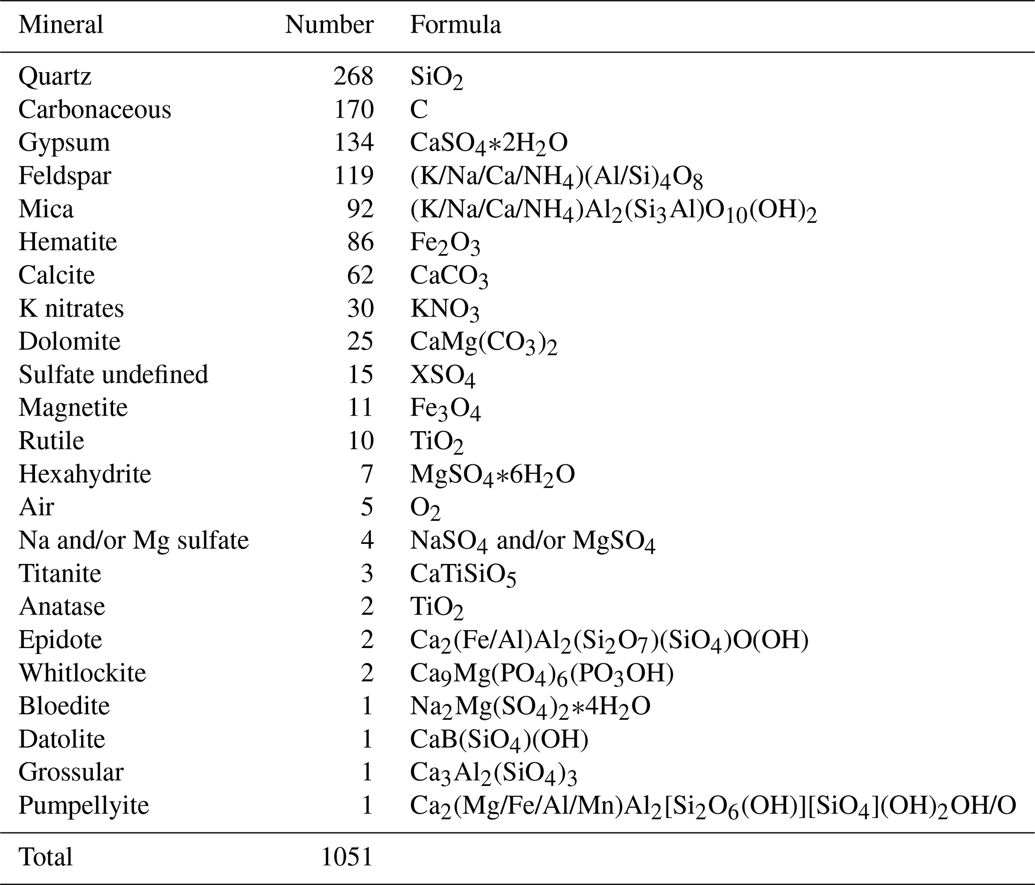
In our 13 samples, we measured 1089 spectra and identified 1051 of them (Fig. 3), resulting in 23 different Raman spectra; 188 micro-inclusions showed luminescence. The chemical formulas of all found minerals are displayed in Table A1.

The most common mineral is quartz (n=268), followed by not further distinguished particles bearing carbon (from here on carbonaceous particles) (n=170) and the sulfate mineral gypsum (n=134). Other sulfate minerals are hexahydrite (n=7), Na and/or Mg sulfate (n=4), bloedite (n=1), and undefined sulfates (n=15). Further minerals are feldspar (n=119), mica (n=92), hematite (n=86), calcite (n=62), K nitrates (n=30), dolomite (n=25), magnetite (n=11), and rutile (n=10). We also identified air (n=5), titanite (n=3), anatase (n=2), and epidote (n=2). Minerals that have not been identified before in ice cores are whitlockite (n=2), grossular (n=1), datolite (n=1), and pumpellyite (n=1); the reference and observed spectra are displayed in Fig. A3.

Figure 3 Identified Raman spectra of micro-inclusions in EGRIP glacial ice; n is the total number of identified spectra per sample. Age shown in white (in ka before 2000 CE) (Gerber et al., 2021). For better visibility, some Raman spectra are condensed into groups. Iron oxides are hematite and magnetite, carbonates are dolomite and calcite, and sulfates include gypsum, bloedite, hexahydrite, Na and/or Mg- and undefined sulfates. Other includes rutile, titanite, anatase, epidote, whitlockite, grossular, datolite, and pumpellyite.

3.3.2 Mineralogy throughout the Last Glacial

We found quartz, carbonaceous particles, feldspar, gypsum, and mica at every depth (Fig. 3). Calcite and the chemically related mineral dolomite occur in S3, S5, S6, S9, S10, S11, and S13. Only dolomite and calcite was found in S4 and S7, respectively. In S6, we identified a total of 27 non-gypsum sulfate minerals, often located in clusters or lined up, in addition to seven gypsum inclusions. Carbonaceous particles are the dominant species in S7, S10, and S13. Hematite was found in 11 of 13 samples, K nitrates in 8 samples, and rutile in 6 samples. The remaining minerals occur at a few specific depths.

In general, there is a decrease in the number of different minerals with depth. Shallow samples (S1–S6) consist of a diversity of 9 to 14 minerals, while deeper samples (S7–S13) consist of a diversity of 6 to 10 minerals per sample (Fig. A6).

In the shallower region of the core, we identified the rarest minerals (n≦3), such as grossular (S1), anatase (S1, S4), epidote (S1, S5), pumpellyite (S2), and whitlockite (S2). Titanite (n=3) is the only rarely observed mineral, which occurs in samples throughout the glacial (S4, S9, and S13).

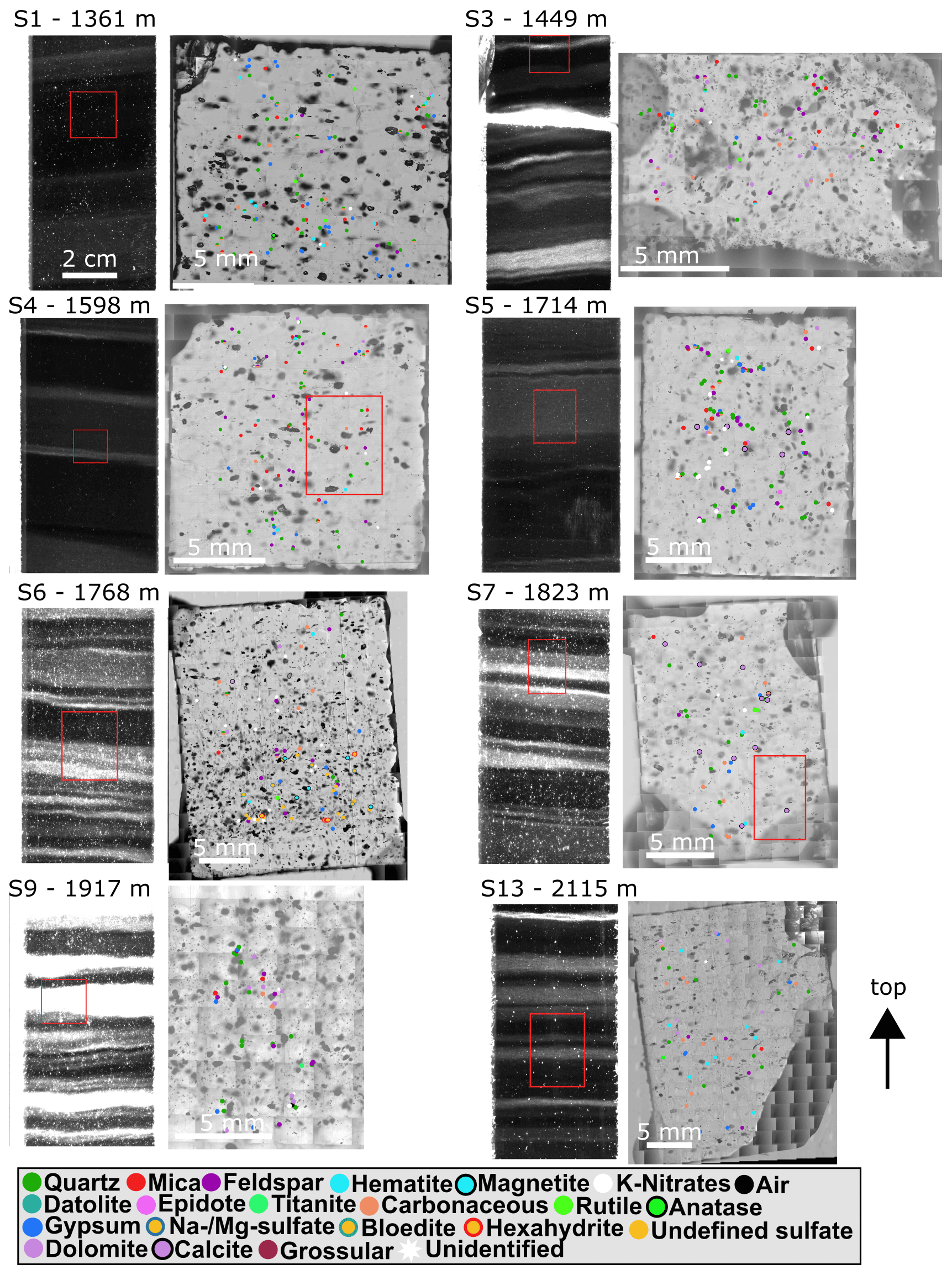
Figure 4 Visual stratigraphy (left) and impurity maps from Raman spectroscopy (right), and red rectangles are the area of Raman analysis. Locations of identified micro-inclusions are indicated by filled circles. Red rectangles in S4 and S7 indicate areas of LA-ICP-MS 2D imaging displayed in Fig. A4.

3.3.3 Localisation of micro-inclusions

Visual inspection shows that most micro-inclusions are in the grain interior. Gypsum and other sulfate minerals in S6 are often located in dense clusters or lined up behind each other. Interestingly, micro-inclusions showing more than one Raman spectra were most often associated with carbonaceous particles, indicating a tight clustering or merging of carbonaceous particles with other minerals. Cloudy bands display a much higher concentration of visible micro-inclusions, while the surrounding darker areas contain comparably few micro-inclusions.

3.3.4 Mineralogy in cloudy bands

The mineralogy in and surrounding the pronounced cloudy bands in samples S6–S11 (Figs. 4, 5, 6, and A1) displays some distinct features. Some minerals, such as hematite and carbonaceous particles, show a distinct localisation inside cloudy bands. S10 is a prime example of this, characterised by a cloudy band in the upper part mainly containing hematite and a thicker cloudy band mainly containing carbonaceous particles in the bottom part of the sample (Fig. 5). The various cloudy bands in S11 (Fig. 6) make it difficult to clearly distinguish between them, but a weak mineral localisation also occurs in this sample. In contrast, the thick cloudy band in S9 consists of different minerals without preferred locations.

Even in samples with faint cloudy bands (e.g. S3 and S13), minerals tend to be localised in specific regions. Carbonates and nitrates are also strongly localised in some samples (S3, S4, S5) but less pronounced than, e.g. hematite. Common dust minerals, such as quartz, mica, and feldspar, are found throughout the samples but occur more regularly inside cloudy bands. Gypsum is also common throughout entire samples and tends to cluster but shows no distinct relation to cloudy bands.

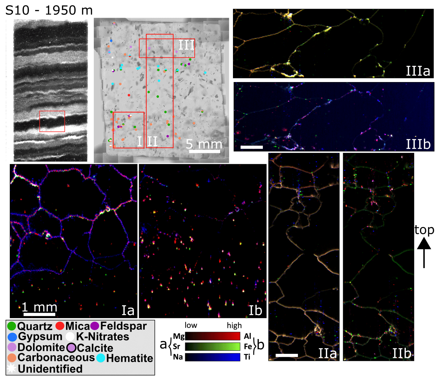
Figure 5 Visual stratigraphy (upper left), Raman spectroscopy (upper centre), and LA-ICP-MS 2D imaging of S10; red rectangles are the area of further analyses. Locations of micro-inclusions identified via Raman spectroscopy are indicated by filled circles. LA-ICP-MS impurity images of the same sample in 20 µm resolution for Mg, Sr, Na and Al, Fe, and Ti indicated by red rectangles and roman numbers in the Raman impurity map; the scale is always 1 mm. Measurements were performed on different days, and thus the analysed surfaces vary.

3.4 Two-dimensional impurity imaging using LA-ICP-MS

We observed strong differences in the microstructural localisation of the analysed elements (Figs. 5, 6). Soluble Na is usually located at grain boundaries. However, in samples containing strong cloudy bands, Na can also be located in the grain interior on some occasions. Mg is predominantly located in the grain boundaries but also occurs infrequently in the grain interior. Al is the prime indicator of insoluble particles (Bohleber et al., 2023) and is found commonly in the grain interior where it often accumulates in particle clusters, i.e. containing several pixels, with additional presence of Ti and Fe. The latter two also show a comparatively weaker presence at grain boundaries, potentially indicating a soluble component. It is important to note that mass 48 (⁴⁸Ti) can also contain a small contribution of Ca, which would also have a substantial soluble component.

Constituting the most important finding, cloudy bands can be clearly distinguished in the chemical images through the presence of insoluble particles mostly indicated by Al, Ti, and Fe at locations that are consistent with the findings from cryo-Raman analysis (S2 and S10 in Figs. 5, 6). Samples with distinct cloudy bands, i.e. S8 and S10, also show a higher amount of impurities in the grain interiors than shallower samples with less distinct cloudy bands, i.e. S2 and S4. The images generally show a high degree of heterogeneity in elemental ratios, indicating a non-homogeneous composition of particle clusters, analogous to the findings by Bohleber et al. (2023).

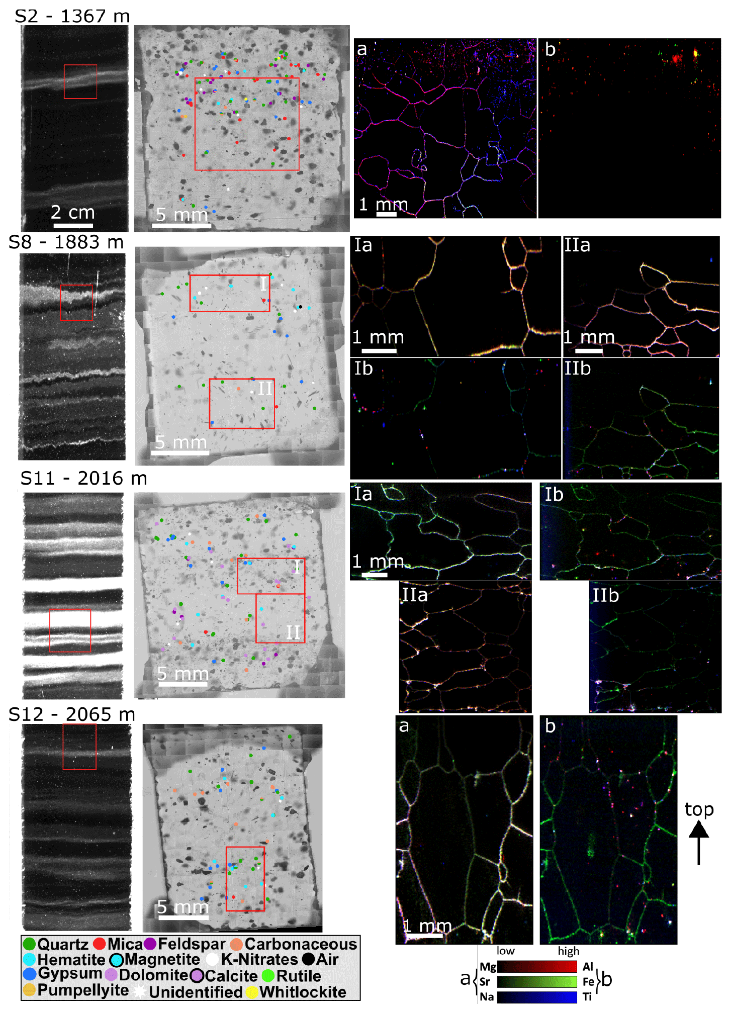
Figure 6 Visual stratigraphy (left), Raman spectroscopy (centre), and LA-ICP-MS 2D imaging (right) of S2, S8, S11, and S12; red rectangles are the area of further analyses. Locations of micro-inclusions identified via Raman spectroscopy are indicated by filled circles. LA-ICP-MS impurity images of the same samples in 20 µm resolution for Mg, Sr, Na and Al, Fe, and Ti are indicated by red rectangles in the Raman impurity maps.

4 Discussion

4.1 Grain size evolution

Mean grain sizes are relatively constant with depth until 1700 m except for the larger grains at 1600 m (Fig. 1). This evolution may be due to sub-grain formation resulting in smaller grain sizes than in shallower ice (e.g. Duval and Castelnau, 1995; Faria et al., 2014). The steady increase in grain size and variability between 1700 and 2121 m is probably due to grain growth and dynamic recrystallisation. Climatic features are visible in the grain size in more detail than in previous studies (e.g. Durand et al., 2006). Grain size changes strongly in Termination 1 (∼15–11 ka b2k) (Fig. 7) and is minimal in the coldest phase of the Last Glacial, i.e. the LGM (∼31–16 ka b2k), likely due to hampered recrystallisation by ice lattice defects caused by the high amount of dust particles and Zener pinning of grain boundaries by particles (e.g. Smith, 1948; Alley et al., 1986; Humphrey and Hatherly, 1996; Durand et al., 2006). Thus, mean grain area and greyscale brightness are often anti-correlated (Fig. 1), displaying the potential impact of high insoluble content on grain size (Stoll et al., 2021b).

The grain size evolution at EGRIP is similar to the NEEM ice core (Montagnat et al., 2014) (Fig. 7) but shifted slightly upwards. This could be related to the different boundary conditions (temperature, elevation) at the drill sites, the impact of extensional deformation and high strain inside NEGIS and the hard shearing in flow direction (Westhoff et al., 2021; Stoll et al., 2021a; Gerber et al., 2023), and the strong dynamic recrystallisation observed at EGRIP (Stoll et al., 2021a). However, the grain size evolution within both cores is still comparable, and the fast-flowing ice within NEGIS does not (yet) intensely affect the grain size in the upper 2121 m (∼80 % of ice sheet thickness).

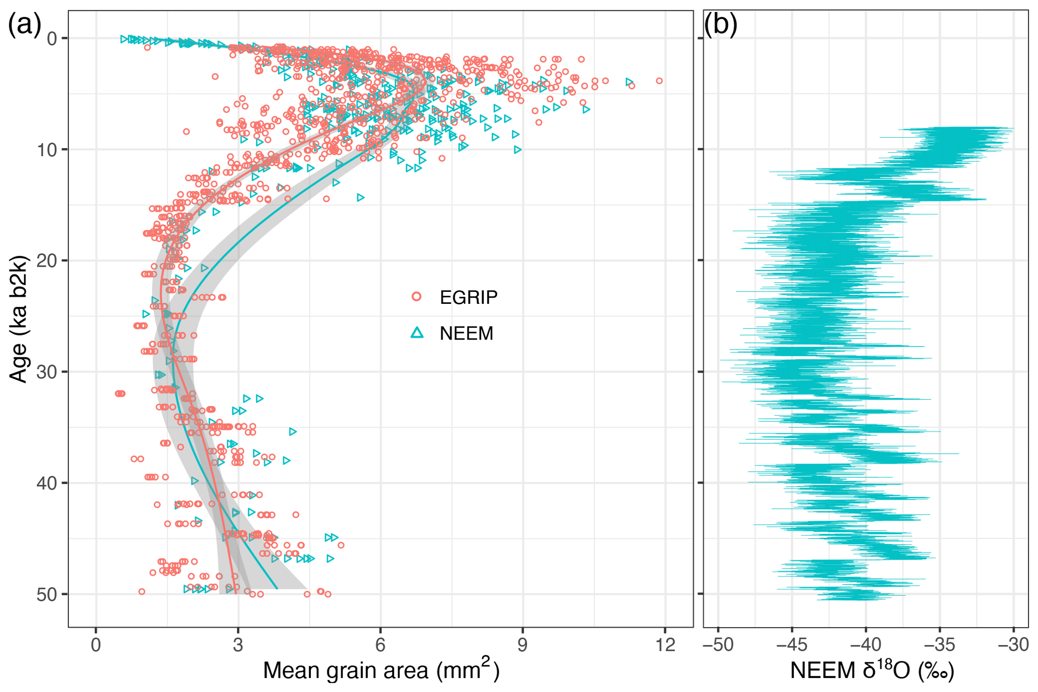
Figure 7 (a) Grain size evolution in the EGRIP (data until 1360 m from Stoll et al., 2021a) and (b) NEEM (Montagnat et al., 2014) ice cores in relation to stable water isotope data. Ages for EGRIP are from Mojtabavi et al. (2020) and Gerber et al. (2021) and ages for NEEM are from Rasmussen et al. (2013). The NEEM stable water isotope δ¹⁸O record is from Gkinis et al. (2021).

4.2 Mineralogy derived via Raman spectroscopy

4.2.1 Mineral diversity

Micro-inclusions in EGRIP glacial ice are mainly terrestrial dust minerals, such as quartz, carbonaceous particles, feldspar, mica, and hematite. Gypsum is also common, and it is the only sulfate found throughout the entire core. Other sulfate minerals only occur in S6, together with eight unidentified spectra. In general, mineral diversity in glacial ice is slightly lower than in Holocene ice (Fig. A6) (Stoll et al., 2022) due to a richer diversity of sulfate minerals in Holocene ice, especially in the shallowest 900 m. Mineral diversity in the glacial is comparably constant and implies a more differentiated trend between the top 900 m and the rest of the core. Together with data from Stoll et al. (2022), mineral diversity decreases with depth, peaks in the intermediate Holocene, and remains relatively constant throughout the Last Glacial. In glacials, specific dust sources dominate, resulting in a uniform mineralogy signature. They suppress smaller dust sources, which thus contribute more to the cleaner atmosphere of interglacials, i.e. the Holocene in our samples, resulting in a higher dust diversity, as seen in our data. Especially samples from intermediate depths, i.e. the LGM, do not show a high mineral diversity (Fig. A6) due to overwhelming dust sources as observed in Antarctica (Gabrielli et al., 2010; Baccolo et al., 2018; Delmonte et al., 2020) and Greenland (Bory et al., 2003; Svensson et al., 2000; Újvári et al., 2022).

4.2.2 Mineralogy and possible inclusion origins throughout 2120 m of EGRIP ice

We show the dominance of terrestrial dust minerals in cloudy bands accompanied by gypsum, carbonaceous particles, calcite, and nitrates. Together with results from the upper 1340 m of the EGRIP core (Stoll et al., 2022), a detailed picture of the mineralogy and its evolution with depth emerges. We show the nine most abundant mineral groups per sample and per climate period in Fig. 8a and b, respectively. Sample numbers in this section thus refer to the sample numbers used in Fig. 8 including results from Stoll et al. (2022). These data enable us to discuss possible source rocks of the observed minerals and geochemical reactions taking place in ice.

The first row in Fig. 8a represents minerals from sedimentary carbonate rocks and traces of wildfire, the second one represents minerals from igneous or metamorphic rocks, and the third one represents trace minerals and minerals possibly (partly) formed in the ice by chemical reactions.

Figure 8 (a) Frequently observed minerals (at least once above 20 % relative share) throughout 24 samples within the EGRIP ice core (the shallowest 11 samples from Stoll et al., 2022). Highlighted lines refer to the specific mineral, and light grey lines reference the other eight minerals. Samples range from 138 m and 1.0 ka (sample 1) to 2115 m and 49.8 ka (sample 24) in depth and age, respectively. Holocene, Younger Dryas (YD), Bølling–Allerød (BO), and the Last Glacial are indicated by different shadings. (b) Pie charts showing absolute numbers of the nine mineral groups in the four analysed climatic periods.

Dolomite and calcite (first row in Fig. 8a) imply that their source rocks are sedimentary carbonate rocks, such as limestone or dolostone. These rocks form by fossil accumulation and organism activity, for example, and involve water and dissolved carbonates. Dolomite and calcite occur for the first time in sample 10 and sample 14, respectively, and only at and below intermediate depths, similar to findings by, e.g. Ohno et al. (2006); Iizuka et al. (2008); Eichler et al. (2019). The dusty atmosphere in glacial times reduces the acidic weathering of mineral particles (during transport and in the ice) because acidic species in the aerosols are neutralised by reacting with the dust. Hence, dolomite occurs abundantly in sample 10 from the dust-rich Younger Dryas and in lower numbers in the deepest samples. Calcite and dolomite are usually found in the same samples, indicating that they are transported together and might originate from similar source regions bearing carbon repositories. Interestingly, we did not find calcite and dolomite in the Bølling–Allerød (Fig. 8a and b).

Carbonaceous inclusions likely originate from wildfires (black carbon) or are pure graphite. They are more abundant in the glacial than in the Holocene where carbonaceous particles were only found in 5 out of 11 samples and were never the dominant species (Stoll et al., 2022). This regular, and comparably high, abundance is due to higher wildfire activity and higher dust loads in the glacial (Han et al., 2020). Our observation of the mixing of carbonaceous particles with other minerals was partly also observed by Eichler et al. (2019), which identified carbon–sulfate mixed particles.

Terrestrial dust minerals, such as quartz, feldspar, and mica, occurring together (second row in Fig. 8a) could imply a fingerprint of their source rocks being of igneous or metamorphic origin, such as granite or gneiss, which mainly consist of these minerals. These rocks are common in the continental crust and available on the surface as the product of weathering (e.g. sand). These dust minerals also display an opposite abundance behaviour to sulfates, especially in the upper seven samples. Quartz, feldspar, and mica peak in sample 5, correlating with a small relative number of sulfates. Below sample 7, this trend is weaker but pronounced in samples 14, 17, and 20 (Fig. 8a).

Hematite (third row in Fig. 8a) originates from weathering in soil, banded iron formations, or places with standing water and can occur in low abundances together with minerals from igneous or metamorphic rocks. Its origin in warm and arid environments (Schwertmann, 1988) thus follows the principal dust sources for Greenland, i.e. the deserts of central Asia. Hematite occurs regularly throughout the core, following its low abundance in rocks but high chemical stability against weathering, with minimum numbers in sample 11 and comparably high numbers in the deepest part of the core (samples 19–24) (Fig. 8a). It is not stable under acidic conditions (pH <4) and dissolves (Schwertmann and Murad, 1983; Zolotov and Mironenko, 2007), thus indicating higher pH values throughout the analysed depth regime. Hematite was found in relatively low amounts throughout the Antarctic TALDICE ice core between MIS3 (31–58 ka) and the Holocene (0–11.7 ka) (Baccolo et al., 2021), which agrees with our findings. However, the hematite amount in EGRIP peaks at 37.3 and 39.9 ka (MIS3) instead of MIS2 as in TALDICE (Baccolo et al., 2021). Similar to Eichler et al. (2019), we only found hematite and not precipitated goethite and jarosite (Baccolo et al., 2021).

Nitrates and sulfates in the third row in Fig. 8a are minerals, which have been recognised as byproducts of weathering processes that involve dust trapped in deep polar ice (Eichler et al., 2019; Baccolo et al., 2021). Nitrates usually originate in arid areas as soil components together with sulfates and sand in, e.g. caliche. Nitrates can also form by chemical reactions in the atmosphere during transport to the ice sheet (e.g. Mayewski et al., 1993; Röthlisberger et al., 2002; Iizuka et al., 2008). Nitrate minerals are usually highly soluble and might react with strong acids in the ice resulting in the solution of NO${}_{\mathrm{3}}^{-}$ (Eichler et al., 2019). In ice, ${\mathrm{NO}}_{\mathrm{3}}^{-}$ is probably relocated to the grain boundaries as solid solution or liquid acid. Thus, solid nitrates can form in the ice by the reaction of ${\mathrm{NO}}_{\mathrm{3}}^{-}$ with chloride salts if there is little H₂SO₄ and carbonate (e.g. Mayewski et al., 1993; Iizuka et al., 2008). A total of 30 inclusions were identified as nitrates at eight depths (S1, S2, S4, S5, S7–S10), which is comparable in number to the 39 nitrates observed in four samples below 899 m (Stoll et al., 2022). We only found single nitrate particles, while Ohno et al. (2005) found compounds containing both nitrates and sulfates.

Sulfate minerals originate in evaporite depositional environments or oxidising zones of sulfide mineral deposits and can be deposited on the ice sheet via dry deposition. The large number of sulfate minerals in the distinct cloudy band at the bottom of S6 (Fig. 4) implies the possibility of dry deposition events unloading sulfate minerals on ice sheets. In ice, sulfate minerals can also precipitate in solid form instead of liquid H₂SO₄ solutions (Iizuka et al., 2008). They are the dominant species in the shallowest seven samples, while they occur less often in deeper samples mainly due to the large variety of different sulfate minerals in the upper 900 m of the EGRIP core (Stoll et al., 2022) (Fig. 8b). Our findings thus support the almost complete absence of sulfate minerals other than gypsum in Greenlandic glacial ice (e.g. Iizuka et al., 2008; Sakurai et al., 2009; Stoll et al., 2022).

Of the minerals, which never had a relative share of above 20 %, only anatase, epidote, magnetite, rutile, and titanite were identified in several samples (Fig. A5). These minerals were probably transported together with more common minerals and are of detrital origin. Especially the minerals observed only at one depth, such as datolite, grossular, prehnite, pumpellyite, pyromorphite, and whitlockite are less abundant in the Earth's crust than frequently observed minerals. Rutile, anatase, and epidote were each only found once similar to observations by Stoll et al. (2022) in shallower EGRIP ice. Whitlockite, pumpellyite, and grossular were identified for the first time in ice cores. These minerals occur all over the globe but are not typical dust minerals and a high number of analysed inclusions is thus necessary to find them. Pumpellyite occurs as a secondary mineral in altered gabbro and basalt and in metamorphic schists. Grossular is part of the garnet group and usually occurs in metamorphosed calcareous rocks. Whitlockite is found in phosphate rock deposits and igneous pegmatites.

4.3 Towards the integration of visual stratigraphy, Raman spectroscopy, and LA-ICP-MS 2D imaging data

Our approach combines data from three methods for the first time. Hence, data integration is far from straightforward. We applied the following structure: (1) a visual characterisation of cloudy bands via visual stratigraphy, (2) an analysis of the localisation and mineralogy of insoluble particles in these defined bands with Raman spectroscopy, and (3) a detailed characterisation of the total impurity content of specific areas with LA-ICP-MS 2D imaging. Integrating chemical data yields results with higher concentrations of impurities (especially insoluble ones) in cloudy bands concurrent with visual data. We further show that insoluble particles are particularly abundant in cloudy bands, strengthening and extending the first steps in combining Raman spectroscopy and LA-ICP-MS 2D imaging (Bohleber et al., 2023). Overlapping LA-ICP-MS with microstructure mapping and Raman spectroscopy data displays that element intensities are higher in cloudy bands than around them (Figs. 5, 6). Additionally, particle clusters with high Fe and Ti intensities are often located where Fe- (magnetite, hematite) and Ti-bearing minerals (rutile, anatase, and titanite) were observed (Figs. 5, 6), supporting the identification of relatively inconspicuous spectra interfered with by the overlying ice spectrum (e.g. magnetite) via Raman spectroscopy. Al, Ti, and Fe vary in concentration throughout samples and are located inhomogeneously (Figs. 5, 6), often as clustered, intra-grain inclusions. Soluble, mobile impurities (Na, Mg, Sr) are at grain boundaries. Some triple junctions display an accumulation of elements while the surroundings are comparably pure. Compared to initial LA-ICP-MS investigations based on spot sizes between 280 and 128 µm (Della Lunga et al., 2014), these detailed insights can only be obtained from high-resolution imaging combined with Raman spectroscopy, expanding previous research (e.g. Ohno et al., 2005; Eichler et al., 2017; Bohleber et al., 2020, 2021; Stoll et al., 2021a, 2022) and marking substantial progress towards a holistic characterisation of microstructural impurity localisation.

4.4 Deciphering the origin of cloudy bands

Our visual and chemical investigations show that cloudy bands are more complex and diverse than previously understood. We here discuss processes involved in their formation. Cloudy bands are commonly interpreted as storm events in spring or summer, transporting large amounts of dust from Asian deserts across the Greenland ice sheet (Svensson et al., 2000). If cloudy bands were solely from dust deposition events in spring and summer, dark layers would dominate the visual stratigraphy. However, the images are dominated by bright layers of high insoluble particle content, as displayed by our Raman spectroscopy and LA-ICP-MS data. The greater thickness of cloudy bands compared to neighbouring dark layers could be due to the high accumulation in spring and summer in Greenland, but this does not explain the observed variation in cloudy band thickness. The abundant unknown cloudy bands at 35, 45, and 48 ka b2k (Fig. 2) all originate from interstadials with low dust concentrations hampering their characterisation.

To understand the anatomy and origin of cloudy bands, the main types of dust deposition are important: (1) dry deposition, i.e. fallout of solid impurities over the ice sheet by atmospheric transportation, and (2) wet deposition, i.e. snowfall and accumulation, including washout of atmospheric dust particles.

Figure 9 Possible processes leading to the identified cloudy band types.

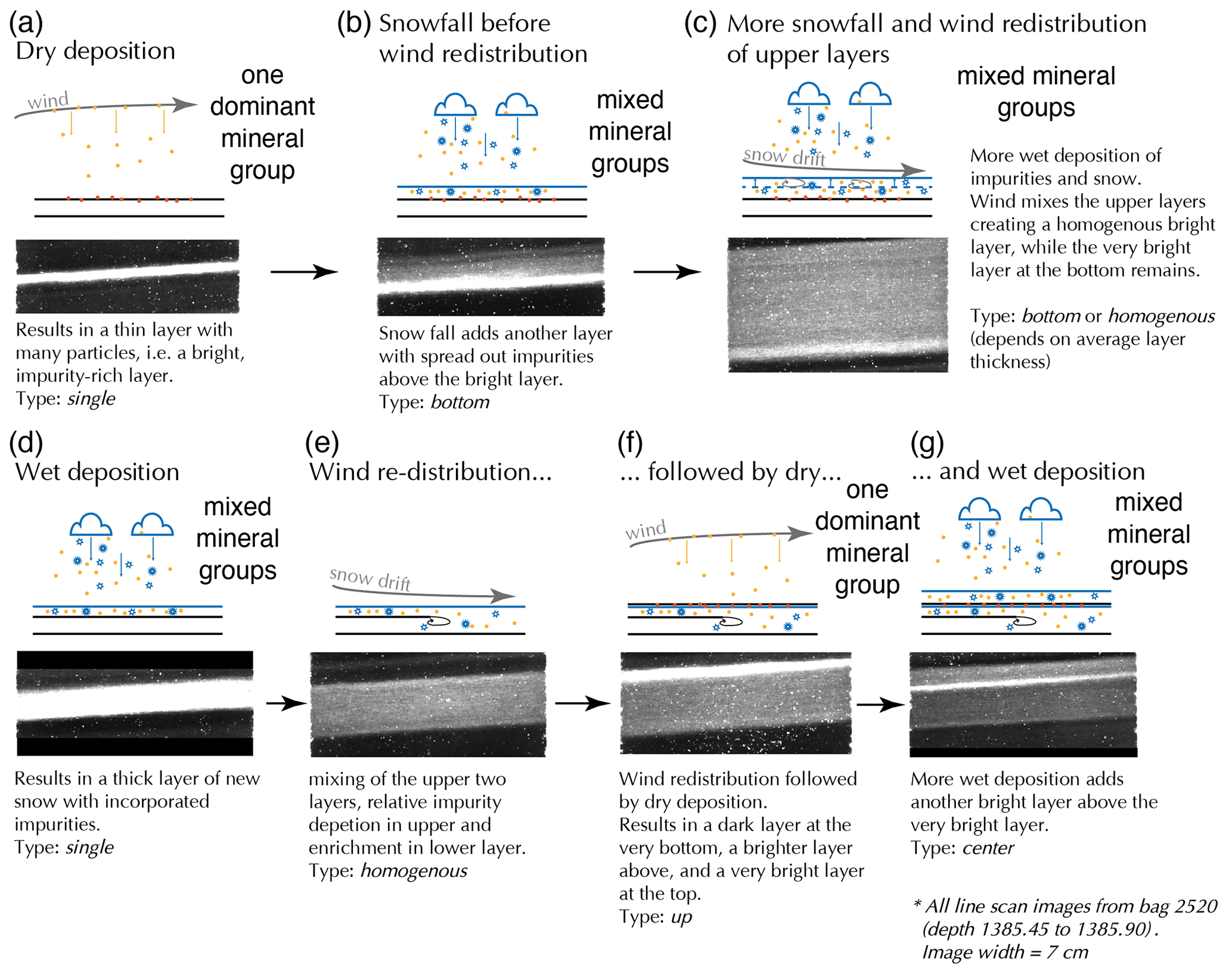
We interpret thin and bright layers (single) as long-lasting dry precipitation events either formed by precipitation or by wind redistribution of surface snow, similar to Svensson et al. (2005). Svensson et al. (2005) further suggest that very thin and bright cloudy bands are associated with enhanced scavenging early in snowfall events or with dry deposition. A single thin and bright layer indicates dry deposition (Fig. 9a), as the layer thickness does not increase by accumulation. Still, dust particles are deposited on the same surface. The greater the number of deposited particles in a single layer, the brighter it appears. Some thin bands show a distinct concentrated layering of insoluble elements and specific minerals, such as hematite and carbonaceous particles, and insoluble elements (Al, Fe, Ti) (S10 in Fig. 5). At low wind speeds, i.e. no redistribution of snow, the thin, dry deposition layer is covered by wet precipitation adding new snow (Fig. 9b). This leads to an increasing layer thickness, resulting in a thick cloudy band (Fig. 9c) with roughly evenly distributed impurities (e.g. S1, S5, S11, S12 in Figs. 4, 6). Snowfall events last a few days, and their sequence thus creates alternating patterns of bright and dark layers (Fig. 9g).

Post-depositional surface processes, such as wind-driven redistribution of surface snow, can lead to well-mixed surface snow layers (Amory, 2020) containing a mix of previously deposited impurities (e.g. S5, S7, and S9 in Fig. 4). Thus, bright and dark layers are mixed into homogeneous and moderately bright layers (Fig. 9d and e). Snow layers impacted by wind redistribution (Fig. 9e) could lead to a homogeneous layer (up, centre, bottom, and confined). Further, wind dunes creating high-density snow layers could serve as lids (Birnbaum et al., 2010) isolating high-impurity layers and creating a distinct type of cloudy band (Fig. 9f), but information on these layers in Greenland is rare. The redistribution and mixing of surface snow by drifting (<2 m above ground level) and blowing (>2 m above ground level) (Amory, 2020) seem to be the main parameters in creating the seven distinguished cloudy band types.

Redistribution of surface snow does not impact variations between seasonal signals in ice cores, as only the seasonal snow is mixed. Mixing snow between different years seems unfeasible, as accumulation in Greenland is high enough for layers to become covered and preserved quickly. Yet this mixing affects the detailed analysis of small-scale distributions of impurities. A single thin cloudy band contains the insoluble particles from dry deposition, maybe including some precipitation, but not significant redistribution by surface processes such as wind. Thick homogeneous cloudy bands are usually dimmer than single thin cloudy bands because their impurity concentration is inhomogeneous due to redistributed surface snow. Dark layers do not contain many visible impurities and thus represent autumn or winter precipitation unmixed with spring or summer layers.

Single bands mostly appear together with dimmer cloudy bands (up, bottom, centre, confined, or heterogeneous). Assuming that a stack of bright layers between two dark layers, i.e. our definition of a cloudy band, represents 1 year, then the most common case is one bright layer per year (single, up, bottom, and centre). In some cases, we find multiple thin and bright cloudy bands within the stratigraphy of 1 year (confined and heterogeneous). The thin cloudy band is missing in other cases (homogeneous). Assuming a constant influx of dust particles over the ice sheet on an annual scale with seasonal variations, the absence of a single thin cloudy band could be a proxy for years with strong surface snow redistribution processes. Cloudy band intensity thus indicates the chronology of events on the ice sheet.

4.5 Outlook

We show the value and future potential of a multi-method and multi-scale approach to better understand the development of cloudy bands. To our knowledge, continuous visual stratigraphy data are rare and only available for the EDML ice core (Faria et al., 2018), potentially enabling a similar study of Antarctic ice. Comparing our results with cloudy bands in NEEM, NGRIP, and RECAP ice is promising. However, the impact of inclusion size, shape, and chemistry on the brightness in the visual stratigraphy needs more research to clarify if deriving more information on impurities from visual stratigraphy is possible. Future LA-ICP-MS applications could be analysing (1) larger areas (several centimetres) covering entire cloudy bands and their surroundings and (2) at higher resolution (1–5 µm) to distinguish analytes in the observed impurity clusters more clearly. Finally, correlating cloudy band types, chemistry, millimetre-scale grain size, borehole deformation, and c-axis orientation data would enlighten us about internal deformation within the EGRIP ice core.

5 Conclusions

Cloudy bands are the main visible feature in glacial ice from deep polar ice cores. They are important but poorly understood factors regarding climatic reconstruction and the internal deformation of ice. With this study, we conducted the first systematic analysis of cloudy bands both in general and specifically in detail using ice from the East Greenland Ice-core Project (EGRIP) ice core accompanied by an analysis of the grain size evolution. We combine visual techniques such as visual stratigraphy, fabric analyser, microstructure mapping, and chemical methods such as Raman spectroscopy and laser ablation inductively coupled plasma mass spectrometry to bridge different spatial scales resulting in new insights into glacial ice, and especially cloudy bands. We identified seven categories of cloudy bands. Single cloudy bands are by far the most abundant ones. However, the relative abundance of cloudy band types differs with depth and the prevailing period (stadial or interstadial). The main minerals in EGRIP glacial ice are quartz, mica, feldspar, gypsum, and carbonaceous particles, which we identified at every depth. The mineralogy is slightly less diverse than in EGRIP Holocene ice. Some cloudy bands show a dominant mineral species (e.g. hematite or carbonaceous particles), indicating a strong deposition event preserved with depth. Laser ablation inductively coupled plasma mass spectrometry 2D imaging shows that cloudy bands are distinguishable from the surrounding ice, and bulk results agree well with other methods. Dissolved analytes, such as Na, are mainly at the grain boundaries; insoluble analytes, such as Fe and Al, are arranged in particle clusters similar to Raman spectroscopy observations. Finally, we elaborate on theories about the origin of cloudy bands based on our chemical and visual observations, thus laying the foundation for future work tackling their direct impact on deformation. Our method can be systematically used in ice core sciences and will provide information on impurity-related processes in the ice, internal stratigraphy, and the dynamics of snow depositions. We demonstrated that the synergetic combination of different analytical techniques is a powerful tool that should be further explored and applied to other ice cores.

Appendix A

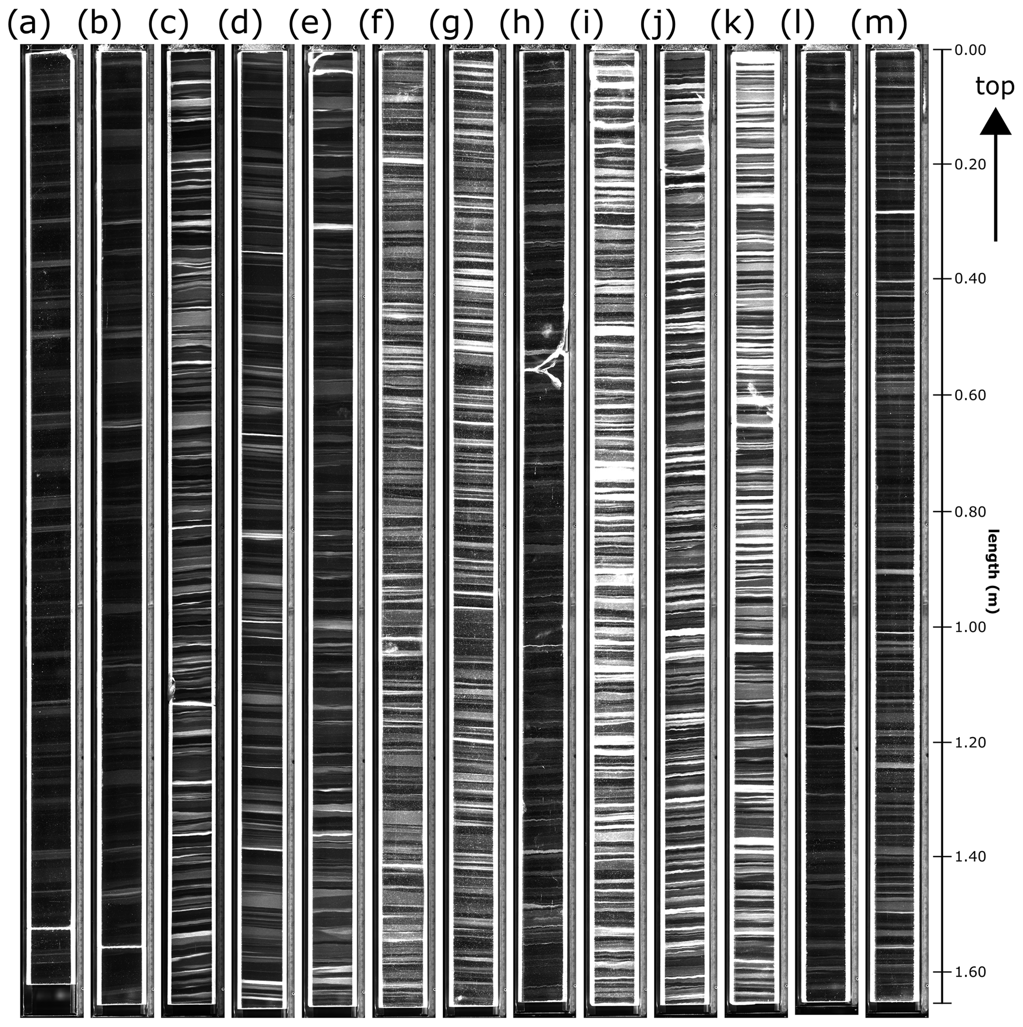
Figure A1 Visual stratigraphy images of the 13 ice core samples partly analysed with Raman spectroscopy. Each sample is 1.65 m long and 8–9 cm wide. Scans consist of three images with different focus planes and apertures. The samples cover the depth regime between 1360 and 2115 m and an age regime between 14.4 and 49.8 ka, i.e. the Last Glacial (Gerber et al., 2021).

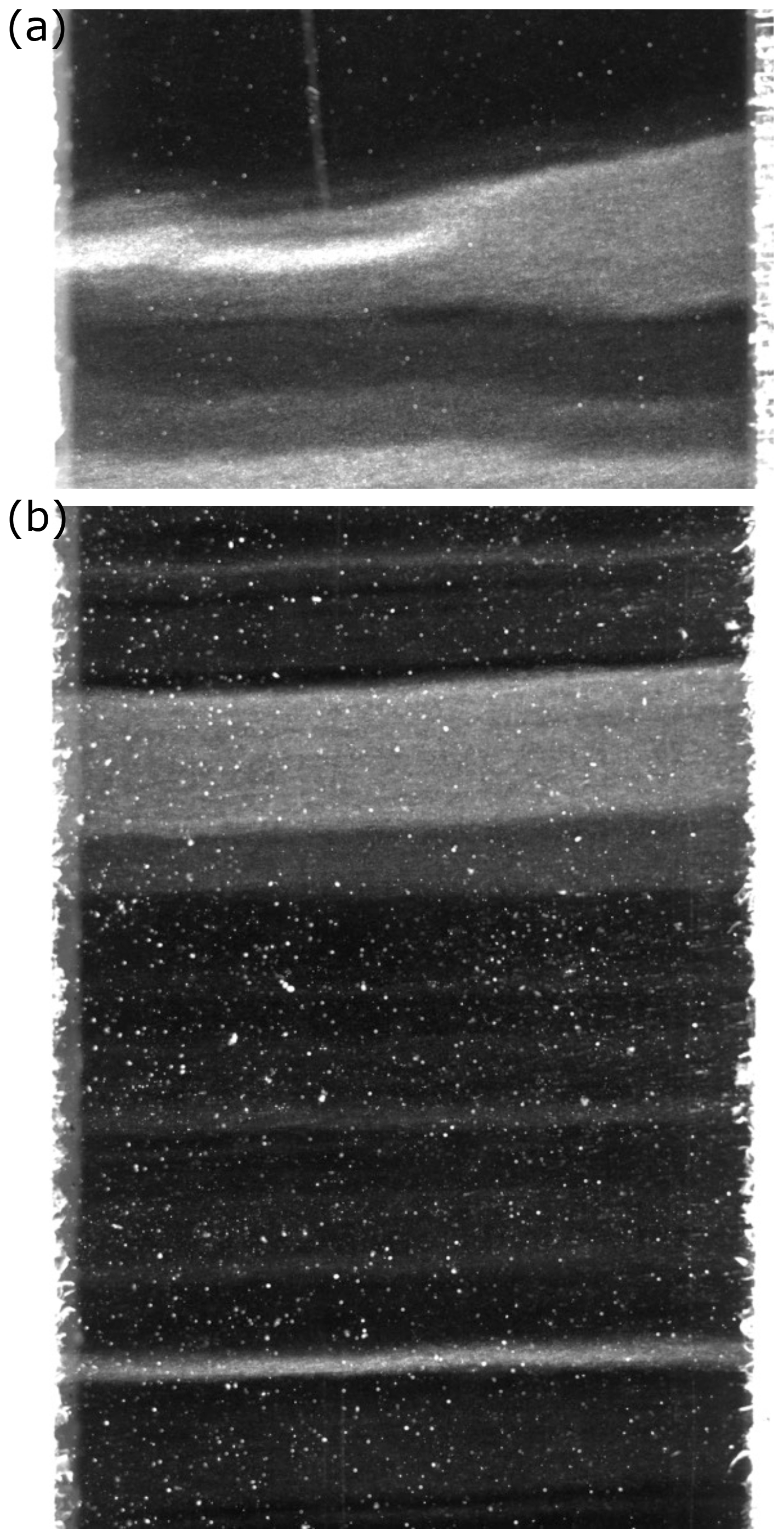
Figure A2 Examples of cloudy bands classified as unknown. (a) The cloudy band fulfils the criteria of being in more than one group. The bright layer on the left side disappears halfway through the cross section; the cloudy band thus belongs to the group centre on the left side and homogeneous on the right side. These cases are rare because we only chose bags with very few folds. Therefore, they are included as unknown to avoid bias in the overview statistic. (b) Distinct cloudy bands at the top of the image, a bright layer with a darker one below, and a thin cloudy band at the bottom. Between these two, we identify at least two dark cloudy bands, which are too dark to classify and thus fall into the category unknown. Enhancing the image brightness would make the cloudy bands visible, yet we refrain from doing this, as all images should be analysed with the same brightness settings.

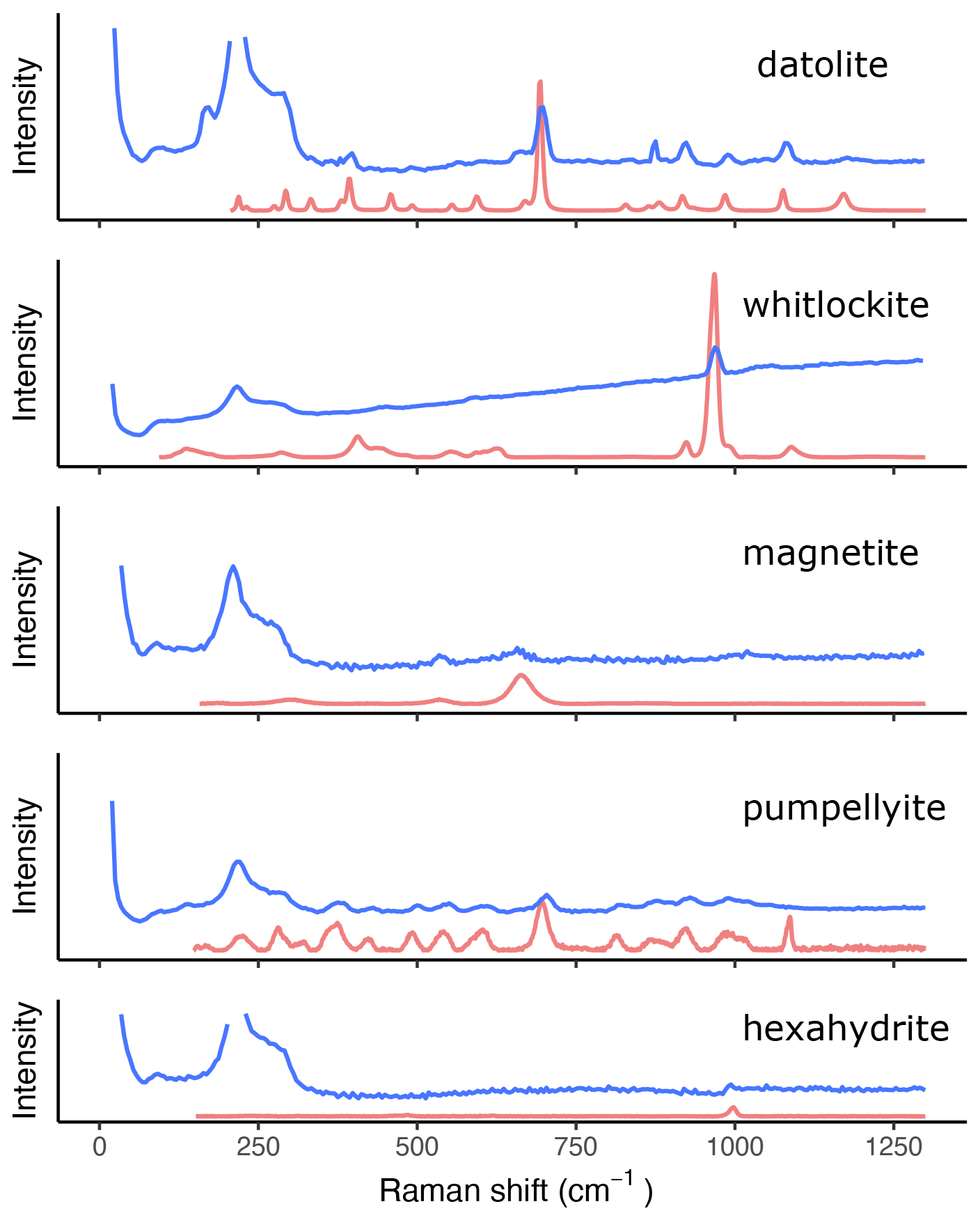
Figure A3 Measured spectra (blue) of datolite, whitlockite, magnetite, pumpellyite, and hexahydrite compared to reference spectra (red) from the RRUFF database (Lafuente et al., 2015). Small deviations are due to the overlaying ice spectrum and differences in the used devices.

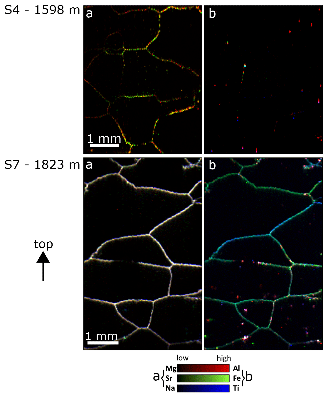
Figure A4 LA-ICP-MS 2D impurity images of S4 and S7 in 20 µm resolution for Mg, Sr, Na and Al, Fe, and Ti.

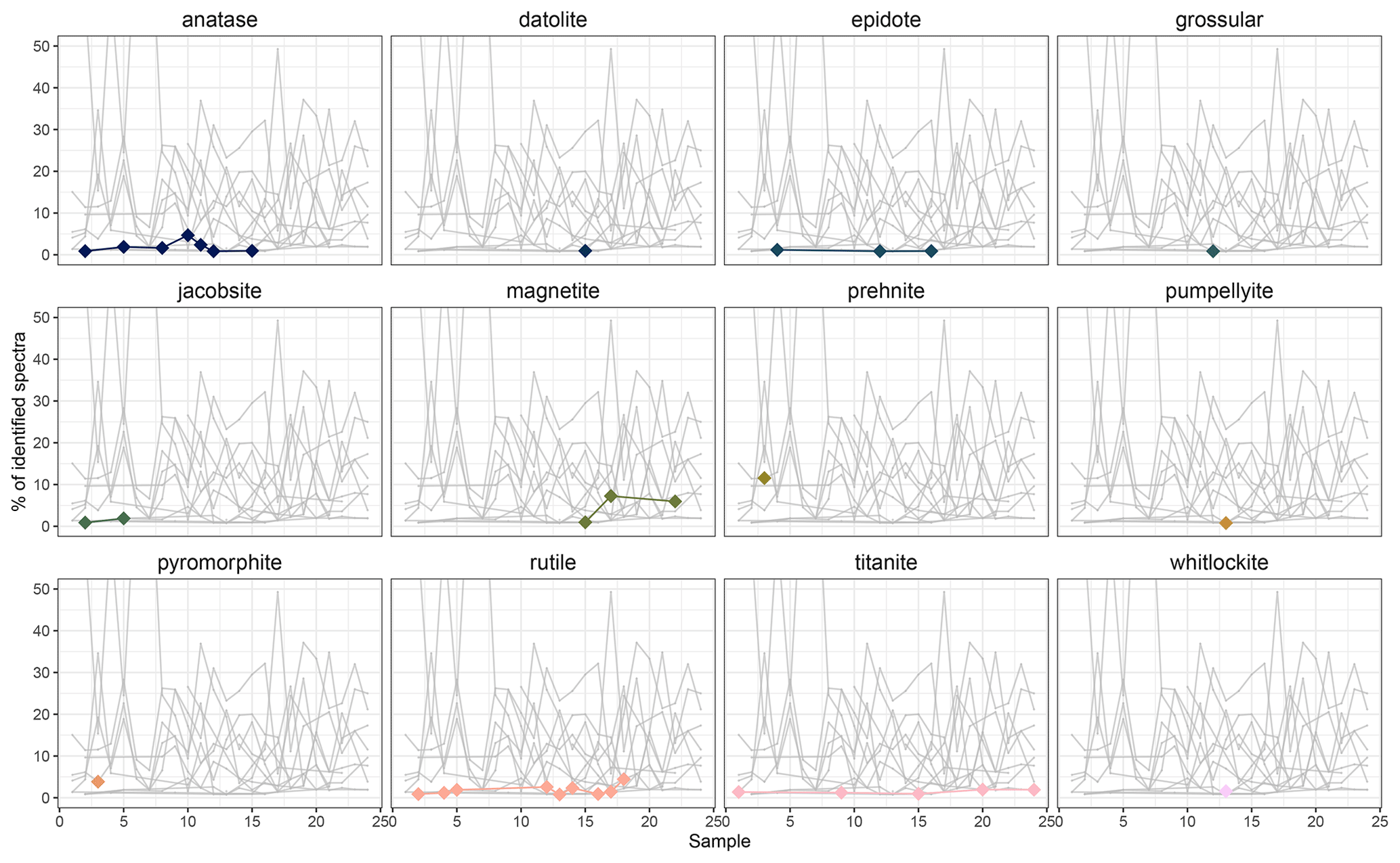
Figure A5 Sparsely observed minerals (always below 20 % relative share) throughout 24 samples within the EGRIP ice core. Data from the first 11 samples from the Holocene from Stoll et al. (2022). Note the changes on the y axes compared to Fig. 8.

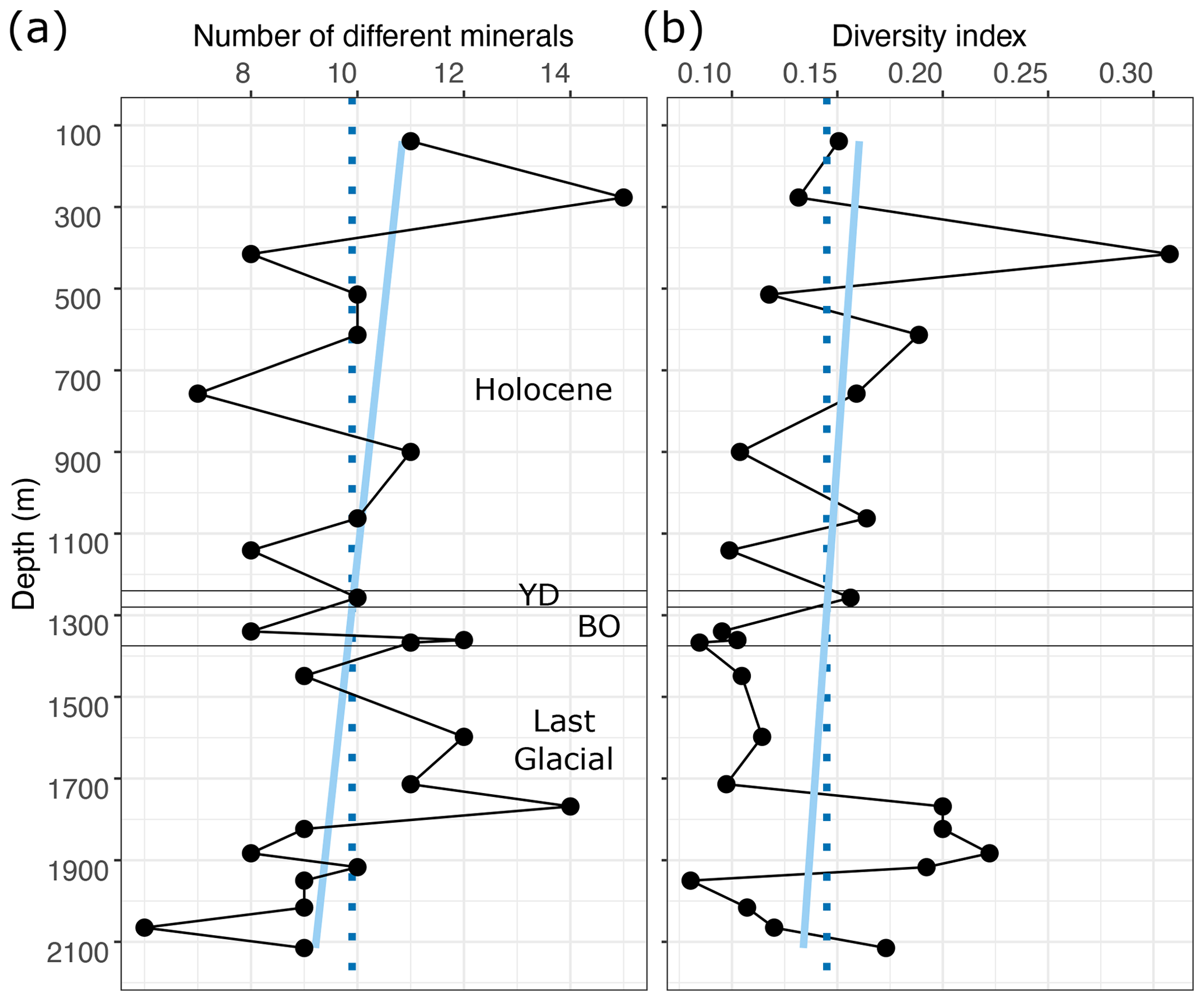
Figure A6 Mineral number and diversity with depth in EGRIP ice down to 2115 m. (a) Absolute numbers of different minerals per sample. (b) Diversity index values calculated following Eq. (1) from Stoll et al. (2022). The light blue lines are linear regressions, and the dotted blue lines are the mean values (a 9.9 and b 0.145). Higher diversity index values indicate a larger mineral diversity in relationship to the amount of identified Raman spectra per sample. YD stands for Younger Dryas, and BO stands for Bølling–Allerød, following Mojtabavi et al. (2020).

Table A1 Identified Raman spectra in EGRIP glacial ice.