Reversible ice sheet thinning in the Amundsen Sea Embayment during the Late Holocene

Cosmogenic-nuclide concentrations in subglacial bedrock cores show that the West Antarctic Ice Sheet (WAIS) at a site between Thwaites and Pope glaciers was at least 35 m thinner than present in the past several thousand years and then subsequently thickened. This is important because of concern that present thinning and grounding line retreat at these and nearby glaciers in the Amundsen Sea Embayment may irreversibly lead to deglaciation of significant portions of the WAIS, with decimeter- to meter-scale sea level rise within decades to centuries. A past episode of ice sheet thinning that took place in a similar, although not identical, climate was not irreversible. We propose that the past thinning–thickening cycle was due to a glacioisostatic rebound feedback, similar to that invoked as a possible stabilizing mechanism for current grounding line retreat, in which isostatic uplift caused by Early Holocene thinning led to relative sea level fall favoring grounding line advance.

1 Overview and background

During the 2019–2020 Antarctic field season, we used a lightweight minerals exploration drill adapted for polar use (Boeckmann et al., 2021) to collect four bedrock cores from 30–40 m beneath the ice sheet surface on the northern side of the Mount Murphy massif, a volcanic edifice located between Thwaites and Pope glaciers in the Amundsen Sea Embayment of West Antarctica (Figs. 1, 2). These and nearby glaciers are experiencing rapid grounding line retreat and thinning, with the result that this sector of Antarctica is the largest contributor to global sea level rise at present (The IMBIE team, 2018; Smith et al., 2020). Retreat and thinning of major Amundsen Sea glaciers is of concern because these glaciers are retreating into overdeepened basins in which ice is grounded well below sea level. Mercer (1978) and, subsequently, many others have proposed that this geometry is inherently unstable because, in general, the rate of ice loss at a marine ice margin increases with the water depth; thus, ice margin retreat into an overdeepening will result in a runaway increase in the retreat rate that continues until the entire overdeepening is fully deglaciated. We refer to this scenario as “irreversible retreat”. As the overdeepening in this case underlies much of the present West Antarctic Ice Sheet (WAIS), this would imply that the present episode of ice thinning and grounding line retreat in this region will inevitably lead to the loss of a large portion of the WAIS, with globally significant sea level impacts. Thus, recent modeling studies (Favier et al., 2014; Joughin et al., 2014; Rosier et al., 2021) have focused on whether or not further retreat inboard of present grounding line positions implies irreversible deglaciation of large segments of West Antarctica. These model simulations and others predict accelerating retreat in the coming decades to centuries, which is consistent with the hypothesis that present grounding line positions are unstable and that irreversible retreat is underway.

The purpose of the drilling program was to apply luminescence dating and cosmogenic-nuclide exposure dating of subglacial bedrock to establish whether or not similar thinning episodes have taken place in the geologically recent past. There is some evidence (Johnson et al., 2022) that portions of the Antarctic ice sheets were thinner than present, with grounding lines inboard of present positions, in the last several thousand years. This implies that past thinning and retreat of grounding lines inboard of present positions in at least some parts of Antarctica were followed by readvance and thickening to the present configuration, rather than continued and irreversible retreat. Thus, determining if and when Amundsen Sea grounding lines have been inboard of their present positions during the geologically recent past is important for understanding the significance of present thinning and retreat. In coastal regions of Antarctica near present grounding lines, ice thickness is closely coupled to grounding line position; therefore, ice thickness changes, which can be investigated by subglacial bedrock exposure dating, are a potential proxy for grounding line position.

Luminescence dating and cosmogenic-nuclide exposure dating of subglacial bedrock are complementary, but not equivalent, methods. Luminescence dating detects past exposure of mineral grains to sunlight (Aitken, 1998). Thus, it can be used to determine whether a rock surface that is ice covered now was ice-free in the past. Detection of past ice sheet thinning using luminescence dating, however, is only possible if the rock surface became completely ice-free (or nearly so, depending on the optical properties of the basal ice). Cosmogenic-nuclide exposure dating, on the other hand, relies on trace nuclides that are produced by cosmic-ray interactions with rocks that are near, but not necessarily exactly at, the surface. Detectable cosmic-ray production extends up to several meters below the ice surface (Dunai, 2010). Thus, it is possible to detect that ice was thinner in the past using cosmogenic-nuclide measurements on subglacial bedrock, even if the rock surface was not completely ice-free.

A much more common use of cosmogenic-nuclide exposure dating is to estimate the deglaciation age of rock surfaces that are ice-free now and were exposed by past deglaciation. This approach has been widely applied to glacial deposits preserved above the present ice surface throughout Antarctica to reconstruct ice sheet change during times in the past when ice sheets were larger than they are now (e.g., Stone et al., 2003). Reconstructing ice sheet change during warm periods when ice sheets were smaller, on the other hand, is necessary for predicting the response to projected climate warming, but it is more difficult because the evidence that an ice sheet was smaller is inaccessible beneath the present ice sheet (Johnson et al., 2022). Here, we show that this obstacle can be overcome by a targeted drilling program.

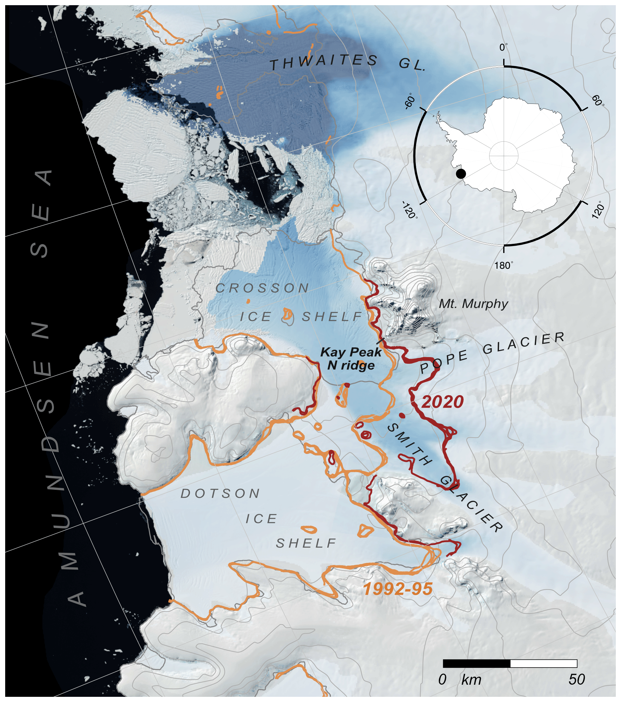
Figure 1 Map of the central Amundsen Sea coast generated using data sets from Quantarctica version 3 (Matsuoka et al., 2021) and showing major glaciers, the drill site at Kay Peak Ridge, and historical grounding line positions in the Thwaites–Pope–Smith Glacier region. The 1992–1995 and 2020 grounding line positions are from Rignot et al. (2011) and Milillo et al. (2022), respectively. The blue shading is a qualitative representation of ice flow velocity and is intended to highlight major glaciers.

Exploiting past exposure of subglacial bedrock as a means of detecting ice sheet thinning is only possible at a site where bedrock is above sea level and thinning will progressively increase the extent of exposed rock adjacent to the ice margin (Spector et al., 2018). The Mount Murphy massif is the only such location in the vicinity of Thwaites and Pope glaciers. On the north side of the massif, several ice-free ridges descend towards Pope Glacier and Crosson Ice Shelf (Fig. 1). At one of these ridges, the north ridge of Kay Peak, a subsidiary peak of the Mount Murphy massif (henceforth “Kay Peak Ridge”), we collected a series of bedrock samples on the exposed part of the ridge from the ice margin to 200 m above the ice surface as well as several bedrock cores from beneath 30–40 m of ice on the subglacial extension of the ridge.

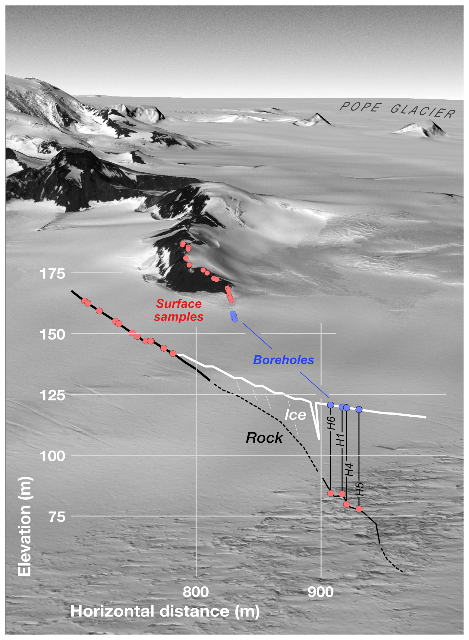
Figure 2 Synthetic oblique view of the drill site at the north ridge of Kay Peak generated from WorldView imagery (© 2018, Maxar) and the Reference Elevation Model of Antarctica (REMA) digital elevation model (Howat et al., 2019). View direction is to the south, as indicated in Fig. 1, from the position of a viewer located over the Crosson Ice Shelf and looking up Pope Glacier. The overlay is an elevation profile along the axis of Kay Peak Ridge showing the relationship between samples collected from the exposed portion of the ridge, drill sites, and subglacial bedrock samples. Note that the vertical scale of the inset profile excludes many samples collected from above 170 m elevation on the ice-free portion of the ridge; Fig. 4 shows the elevation distribution of the entire sample set.

Observations in recent decades show that the ice thickness at Kay Peak Ridge is likely coupled to the position of the grounding line of Pope Glacier. Like Thwaites Glacier, Pope Glacier has experienced rapid grounding line retreat in recent decades, from immediately adjacent to our drill site in 1992–1995 to ∼10 km landward of the site in 2014 (Fig. 1; Milillo et al., 2022). Correspondingly, comparison of 1966 aerial photographs with 2018–2019 satellite imagery indicates expansion of the area of exposed rock on the ridge, which requires thinning of adjacent ice by at least 31 m in 52 years (Fig. 3). Lacking surface mass balance data for the 1966–2020 period, it is not possible to conclusively prove that ice thinning at the drill site is solely a dynamic response to nearby grounding line retreat, but the coincidence of thinning and retreat is consistent with a grounding line control on ice thickness in this area.

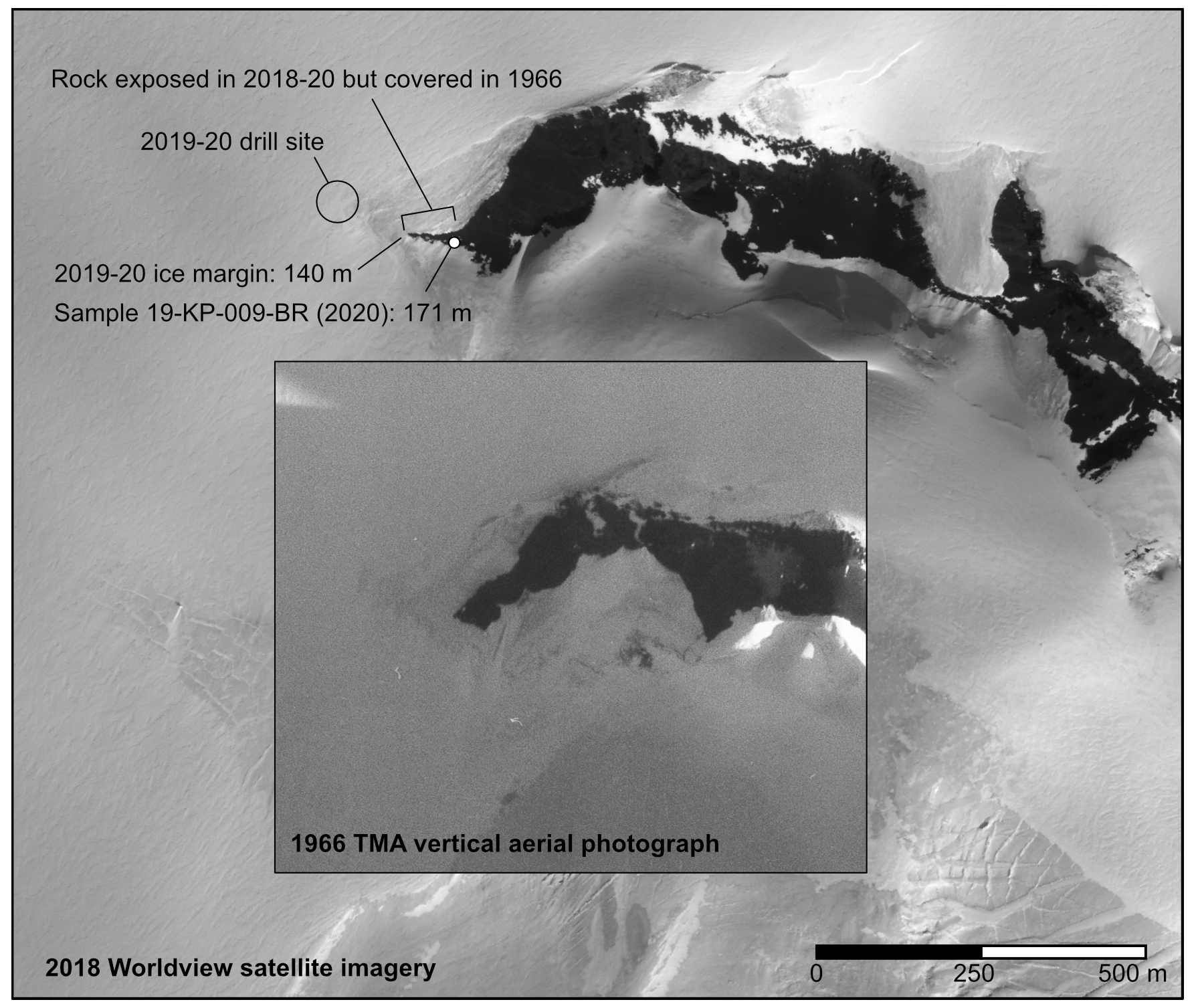
Figure 3 WorldView satellite imagery (© 2018, Maxar) collected on 8 December 2018 (main image) showing the north end of Kay Peak Ridge, compared with a US Navy vertical trimetrogon aerial (TMA) photograph (inset image) taken on 5 January 1966 (TMA1720, frame 231V). The 1966 photograph is not geolocated, so the images were adjusted to a common scale by matching bedrock features on the lower ridge. This comparison does not attempt to correct for look angle, so comparison of the extent of exposed rock is not quantitative. However, the shape of the ice margin clearly indicates that a portion of the lower ridge exposed in 2018 was not exposed in 1966. In fieldwork in 2019–2020, we collected samples from the portion of the ridge that was ice covered in 1966 and surveyed sample locations and the lowest exposed rock on the ridge using a combination of handheld GPS, differential GPS, and barometric elevation measurements. Based on the image comparison, the highest sample that was clearly ice covered in 1966 has a present elevation of 171 m. As the present ice margin is at 140 m elevation, the elevation of the ice margin decreased at least 31 m between 1966 and 2020.

Exposure-age data from the ice-free portion of the ridge, collected in previous research (Johnson et al., 2020) and supplemented by additional measurements in this work (Methods 2 and Tables S1 and S5 in the Supplement), include measurements of ¹⁴C and ¹⁰Be produced in situ in quartz (Fig. 4). The important difference between ¹⁴C and ¹⁰Be exposure ages is that the 5700-year half-life of ¹⁴C precludes the survival of any significant ¹⁴C concentration from surface exposure prior to the Last Glacial Maximum (LGM) 15 000–25 000 years ago. Although measured ¹⁰Be concentrations could be, and often are, the result of surface exposure during both the present interglaciation and one or more previous ones, ¹⁴C can only be the result of post-LGM exposure (Nichols et al., 2019). As described by Johnson et al. (2020), ¹⁰Be exposure ages from bedrock and erratics on Kay Peak Ridge are spuriously old due to ¹⁰Be inheritance, but ¹⁴C exposure ages from the ridge agree with a large set of other data from the overall Mount Murphy massif in recording progressive exposure of the ridge by Early Holocene ice sheet thinning from 200 m above the present ice surface at 6–10 ka to near present conditions at 4–7 ka. The ¹⁰Be exposure ages from a nearby small outcrop 1 km to the west of Kay Peak Ridge (Fig. 4; Adams et al., 2022) also indicate deglaciation at 6–7 ka. Although the ¹⁴C exposure ages from Kay Peak Ridge scatter more than expected from measurement uncertainties, likely because of the complex effect of both regional ice surface lowering and the retreat of fringing ice fields in uncovering the ridge axis, they agree with other exposure-age data sets throughout the Amundsen Sea region that uniformly show rapid Early and Middle Holocene thinning reaching the present ice surface between 4 and 7 ka (Johnson et al., 2014, 2020). Early Holocene thinning was associated with, and presumably caused by, the coeval retreat of glacier grounding lines across the adjacent continental shelf (Hillenbrand et al., 2017).

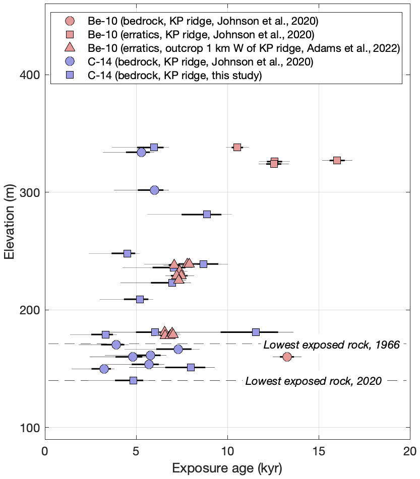
Figure 4 Apparent ¹⁰Be and ¹⁴C exposure ages for bedrock and erratic samples from the ice-free section of Kay Peak Ridge, including data already published in Johnson et al. (2020) and additional measurements in this study (see Methods 2 and Tables S1 and S5 in the Supplement). All data are also available through the ICE-D:ANTARCTICA database at http://www.ice-d.org (last access: 22 April 2023). Apparent ¹⁰Be exposure ages from an adjacent outcrop 1 km west of Kay Peak Ridge, described in Adams et al. (2022), are also shown. Error bars indicate the 68 % (thick line) and 95 % (thin line) confidence intervals. “Apparent exposure ages” are exposure ages calculated from measured nuclide concentrations with the assumption that samples have experienced a single period of exposure at their present location without burial or surface erosion.

There are no exposure-age data in the Amundsen Sea region indicating thicker than present ice after 4 ka (Johnson et al., 2022). Thus, existing observations require either (i) zero change in ice thickness in the last several thousand years or (ii) continued thinning below the present ice surface, followed by thickening to the present configuration. Zero change in ice thickness for millennia appears unlikely given dynamic Late Holocene boundary conditions, including relative sea level (RSL) change forced by eustatic and glacioisostatic effects, climate and oceanographic changes (Walker and Holland, 2007; Hillenbrand et al., 2017), and changes in grounding line position elsewhere in Antarctica (Venturelli et al., 2020; King et al., 2022). In addition, apparent ¹⁴C exposure ages of 4–7 ka on samples below the 1966 ice surface (Fig. 4) require at least some period in the Holocene during which the ice was thinner than it was in 1966.

Relative sea level in coastal Antarctica rose between the LGM and Early Holocene because meltwater addition to the ocean from disintegrating LGM ice sheets outpaced local isostatic rebound, but this relationship reversed in the Late Holocene as global ice volume stabilized but isostatic equilibration to Early Holocene mass loss was not yet complete (Lambeck et al., 2014). As relative sea level is a primary control on grounding line position at marine ice margins (e.g., Gomez et al., 2010), this sequence of events predicts grounding line advance and associated thickening in the Late Holocene (Johnson et al., 2022), and isostatic response to ice sheet thinning has also been proposed as a potential stabilizing feedback for present grounding line retreat and thinning (e.g., Barletta et al., 2018). The aim of the drilling program was to determine if this process was active in the past by detecting and, if present, quantifying a hypothesized Holocene thinning–thickening cycle.

2 Drilling and sample collection

We located the subglacial extension of Kay Peak Ridge using ice-penetrating radar. Ice within ∼200 m of the lowest exposed rock on the ridge was crevassed and unsafe for drilling, so the survey began at the closest accessible point to the exposed ridge, where ice was ∼25 m thick, and extended away from the ice margin until the ridge crest was below the depth feasible for drilling (∼60 m). This identified an approximately 70 m long section of subglacial ridge where drilling was possible (Figs. 2, 5).

We conducted the survey with a ski-towed radar system consisting of a Geophysical Survey Systems, Inc. (GSSI) SIR 4000 control unit and model 3108 100 MHz monostatic transceiver, coupled to a Garmin GPSMap 78 handheld GPS unit. We also installed a series of snow stakes in a 70 m × 100 m grid with 10 m spacing overlying the subglacial ridge and marked these stakes on radar profiles collected along grid lines (Fig. 5). This provided higher-resolution spatial referencing than possible using the GPS alone. The antenna was oriented perpendicular to the direction of travel and towed at approximately 1 km h⁻¹. Scans were recorded for 2400 ns with 1024 32-bit samples per scan and 30–50 scans per second, translating to ∼90 scans per meter. Data were recorded with range gain and post-processed with (i) high-pass (25 MHz) and low-pass (300 MHz) filters to reduce noise, (ii) distance corrections based on the 10 m spaced grid stakes, and (iii) stacking (5–10 stacks) to improve the signal-to-noise ratio. We then applied a basic Kirchhoff migration of the data using hyperbolae from bedrock and internal reflectors to estimate relative permittivity as well as associated velocities and depths to bedrock. We did not apply more advanced processing techniques in the field because the survey was conducted immediately (1 d) before we began drilling. Hence, we selected drill sites as close as possible to the ridge axis by locating the apparent high point on each ridge crossing in the migrated data.

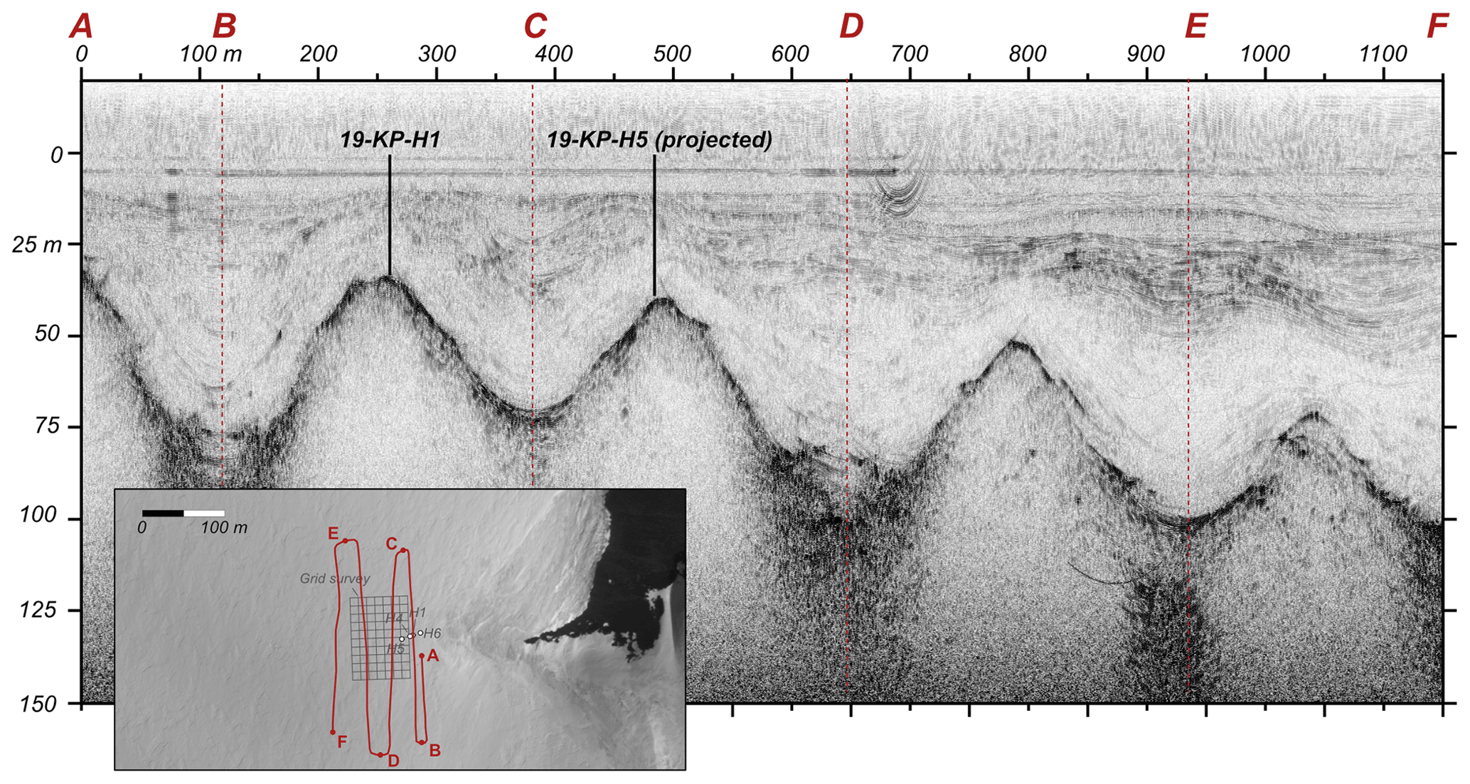
Figure 5 Example 100 MHz radar profile collected prior to drilling in 2019–2020 that crosses the subglacial portion of Kay Peak Ridge four times (see inset map). The profile has been distance normalized, and a Kirchhoff migration was applied to improve bedrock depth estimates. Core 19-KP-H1 lies on the radar line, as shown, and the nearest projected location of 19-KP-H5 is also shown. The projected locations of two other cores, 19-KP-H4 and 19-KP-H6, would be near 19-KP-H1 in this figure. The location of the grid survey that was also used for drill site selection is shown in gray.

We collected subglacial bedrock samples using a two-stage drilling process. First, we made an access hole through the ice, extending as close as possible to the bedrock surface, using a Badger-Eclipse cable-suspended ice core drill, which produces a 113 mm borehole. Drilling with this system stopped when the sediment concentration in basal ice became high enough to dull the cutting bit and halt progress. We then occupied the access hole with a “Winkie” pipe-string, normal circulation compact rock coring drill, modified for polar use by the US Ice Drilling Program (Boeckmann et al., 2021). We set casing in the ice at the bottom of the access hole using an inflatable packer to enable fluid circulation and cored through the remaining sediment-rich basal ice into underlying bedrock. The ice–bedrock interface was frozen at all core sites, and we did not observe loss of drilling fluid into the ice–bed interface.

We reached bedrock 36–41 m below the surface at four boreholes (Fig. 2, Table S1). In all boreholes, we observed a firn–ice transition 12–17 m below the surface and then a transition from clean glacier ice to a 40–120 cm layer of sediment-rich basal ice in contact with bedrock. Note that the presence of debris-rich, optically opaque basal ice is important in this study because resetting of luminescence signals could not occur through thin ice; detection of ice thinning using luminescence dating would require complete removal of basal ice and direct sunlight exposure of the bedrock surface. At three holes, we recovered 114–137 cm long, 33 mm diameter cores of the underlying bedrock, whose lithology is a biotite gneiss identical to the bedrock exposed at the ice margin. At the fourth borehole (19-KP-H6) we recovered 7 cm of fragmented rock with the same lithology. However, this section of the core included fragments of both rock and debris-rich basal ice, so it was not possible to determine whether this sample represented (1) part of a densely jointed or rubbly bedrock surface or (2) one or more loose clasts within the basal ice. At two of the boreholes, we were able to extract bedrock core tops from the core collection barrel within a lightproof bag so that they were not exposed to sunlight, permitting infrared stimulated luminescence (IRSL) measurements on the bedrock surface. In the next sections, we describe IRSL measurements on two core tops and measurements of the cosmic-ray-produced radionuclides ¹⁰Be, ¹⁴C, and ²⁶Al in quartz from three cores.

3 Infrared stimulated luminescence (IRSL) depth profiles

3.1 Methods

We made IRSL depth profile measurements (Sohbati et al., 2011, 2012) in the uppermost 4 cm of the two core top samples that we were able to remove from the core barrel without exposure to sunlight (19-KP-H1 and 19-KP-H4). In addition, to establish kinetics of bleaching during sunlight exposure for this lithology, we collected equivalent depth-profile data on a rock surface above the present ice margin that had been newly exposed by collection of a rock sample 4 years earlier (Johnson et al., 2020).

Depth-profile measurements were made by slicing rock samples parallel to the exposed surface using a low-speed, water-cooled lapidary saw with a 0.38 mm fine-kerf blade. Each slice was then approximately broken into quarters, each of which was disaggregated using gentle crushing in a mortar and pestle to yield mineral grains suitable for IRSL measurement, and all were analyzed separately in order to better capture the natural variability in the luminescence response at each depth. We then used a post-infrared infrared-stimulated luminescence (pIRIR) protocol (Buylaert et al., 2009) to determine sensitivity-corrected natural luminescence intensities ($L_{\mathrm{N}}/T_{\mathrm{N}}$) as well as the dose response and fading characteristics of each sample. This pIRIR protocol yields measurements of two luminescence signals: the more bleachable IR₅₀ signal, which originates from both Na- and K-rich feldspars and has higher signal-fading rates, and the less bleachable pIRIR₂₂₅ signal, which is mostly from K-rich feldspars and fades less (Thomsen et al., 2018). Further details of the measurements are given in Methods 1 and Table S2 in the Supplement.

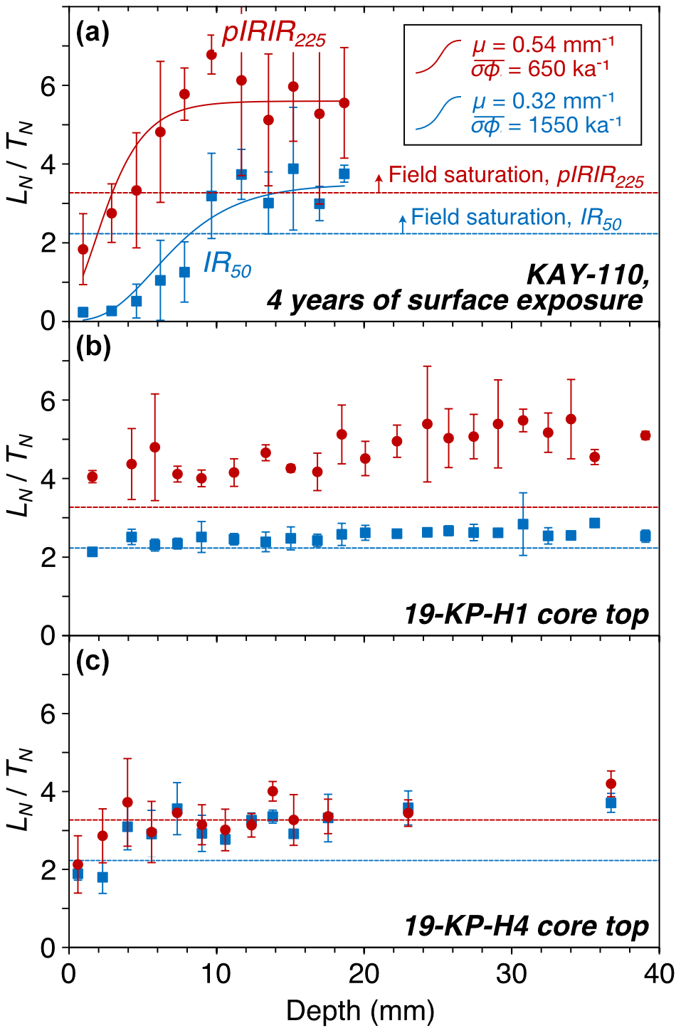
Figure 6 Sensitivity-corrected luminescence intensity for the IR₅₀ and pIRIR₂₂₅ signals, with the IR₅₀ signal being more bleachable when exposed to sunlight. The depth profiles for both signals in both core tops (b, c) are indistinguishable from field saturation, the 95 % confidence level for which is indicated with horizontal dashed lines. By comparison, KAY-110 (a), which was exposed to sunlight for 4 years prior to measurement, shows reduced intensity near the surface due to signal bleaching. For KAY-110, solid lines show a bleaching model fitted to the data to yield estimates of the detrapping rate at the rock surface, $\stackrel{\mathrm{‾}}{\mathit{\sigma }\mathit{\varphi }}$ (ka⁻¹), and the sunlight attenuation coefficient, μ (mm⁻¹) (Methods 1 and Table S2 in the Supplement).

3.2 Results

The depth profile in the surface sample shows significant bleaching, manifested as values of $L_{\mathrm{N}}/T_{\mathrm{N}}$ for both luminescence signals that approach zero at the surface and are significantly below field saturation values in the uppermost 1 cm, after 4 years of exposure (Fig. 6). If the core tops had been exposed to sunlight during the Holocene, they would also show values of $L_{\mathrm{N}}/T_{\mathrm{N}}$ systematically below saturation at shallow depths. They do not. Rather, IRSL signals in core tops are indistinguishable from calculated field saturation at all depths. This means that the bedrock surfaces of the core tops were not exposed to sunlight during the period required to approach saturation. We estimate the period required to approach saturation as 200–280 kyr based on estimated dose rates and measured fading properties (Methods 1 in the Supplement). Therefore, bedrock at these two core sites was not ice-free during the Holocene.

4 Cosmogenic-nuclide measurements

4.1 Methods

We sectioned bedrock cores into 10 cm segments, separated quartz from each segment, and measured concentrations of cosmic-ray-produced ¹⁰Be and ¹⁴C in quartz separates from three cores as well as ²⁶Al in quartz from one core. As discussed above in the introduction, the purpose of measuring multiple cosmogenic nuclides in the core samples is to distinguish Holocene from pre-Holocene exposure of bedrock. ¹⁰Be and ²⁶Al have relatively long half-lives (1.4 and 0.7 Ma, respectively); thus, if the core sites were not affected by subglacial erosion during the LGM, ²⁶Al and ¹⁰Be produced in near-surface rocks in a previous ice-free period prior to the LGM could be preserved to the present. Observing cosmogenic ¹⁰Be or ²⁶Al in subglacial bedrock would prove that the surface had been exposed at some time in the past, but it would not prove that the surface had been exposed in the Holocene. In contrast, ¹⁴C has a half-life of 5700 years, so ¹⁴C produced prior to the LGM would be removed by radioactive decay. Cosmogenic ¹⁴C observed in subglacial bedrock unambiguously requires Holocene exposure.

In brief, ²⁶Al and ¹⁰Be analysis employs an isotope dilution method in which quartz is dissolved in hydrofluoric acid in the presence of a known quantity of the common isotopes ⁹Be and ²⁷Al, Be and Al are separated by column chromatography, and ¹⁰Be and ²⁶Al concentrations are quantified by accelerator mass spectrometer (AMS) measurement of the ${}^{\mathrm{10}}\mathrm{Be}{/}^{\mathrm{9}}\mathrm{Be}$ and ${}^{\mathrm{26}}\mathrm{Al}{/}^{\mathrm{27}}\mathrm{Al}$ ratios. ¹⁴C produced in situ in quartz is measured by fusing quartz with a lithium metaborate flux in a high-purity O₂ atmosphere to release ¹⁴C as CO₂, followed by CO₂ purification, barometric measurement of the total amount of CO₂, and conversion to graphite for AMS measurement of the ${}^{\mathrm{14}}\mathrm{C}{/}^{\mathrm{12}}\mathrm{C}$ ratio. The detection limit for all three nuclides is quantified by measurement of process blanks. The ¹⁰Be and ²⁶Al concentrations in core samples are 2000–7000 and 16 000–44 000 atoms g⁻¹, 2–5 times the detection limit inferred from process blanks and within the range routinely measured for exposure-dating applications. The ¹⁴C concentrations in quartz in the core samples are in the range of 10 000–50 000 atoms g⁻¹. These concentrations are 2–3 times the typical detection limits for in situ ¹⁴C in quartz, but they are significantly lower than routinely measured. Thus, we characterized the distribution of process blanks by analyzing 50 process blanks during the period in which sample analysis took place. In addition, we made replicate analyses of multiple aliquots of quartz for nearly all samples. Analytical methods, blank-correction procedures, and determination of detection limits are described in detail in Methods 2 and Tables S3–S5 in the Supplement as well as in Balco et al. (2022).

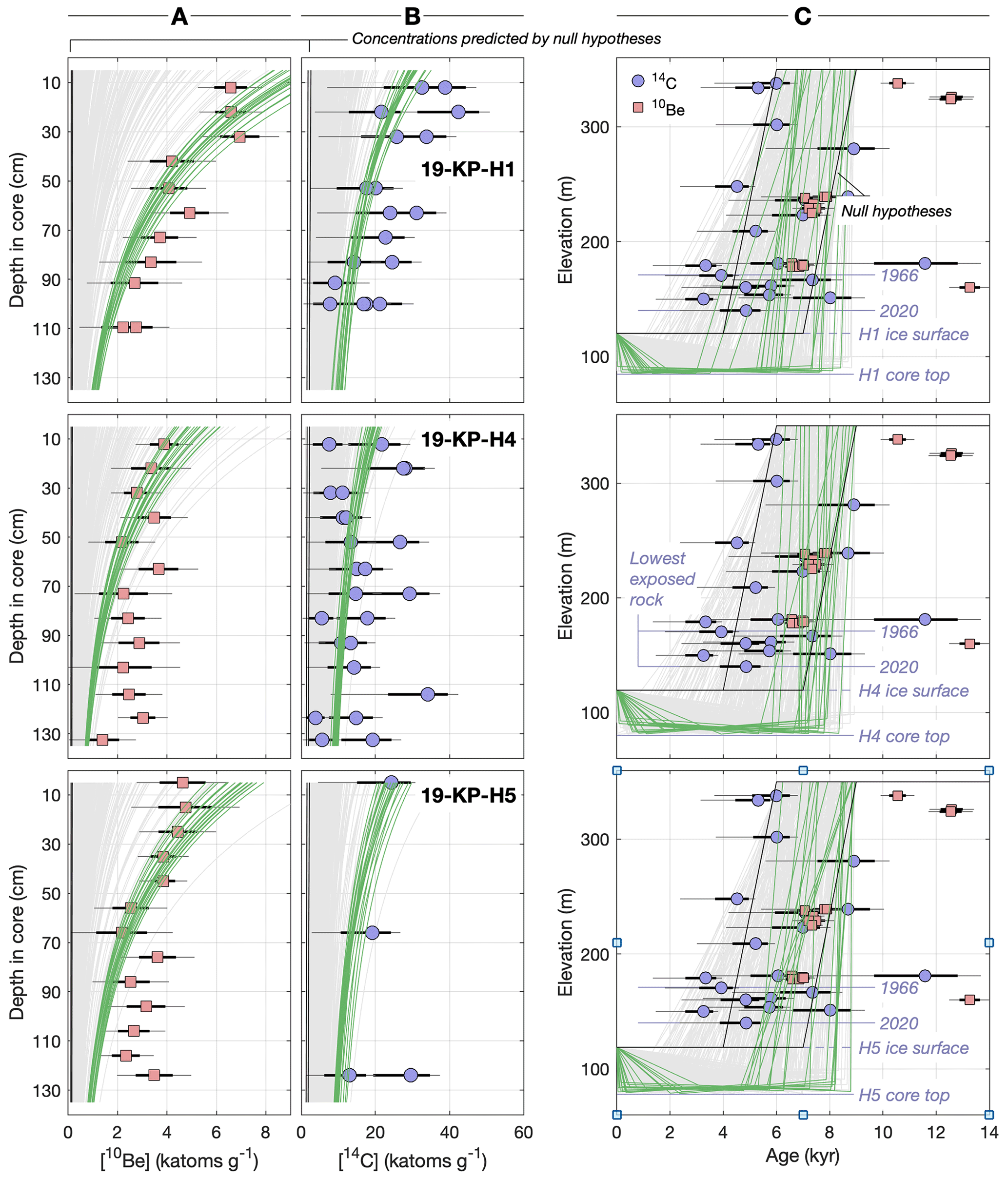
Figure 7 ¹⁰Be and ¹⁴C concentrations in core samples compared to the null hypothesis for zero Holocene thinning and to results of the random search algorithm. Columns (a) and (b) compare measured and predicted in situ ¹⁰Be and ¹⁴C concentrations in quartz in three subglacial bedrock cores. Green and gray lines show concentrations predicted by ice thickness change histories generated by the random search algorithm that best fit data from each core. Results shown in green are the best-fitting 1 % of the random search iterations, and others are shown in gray. Likewise, column (c) compares the thickness change histories that do and do not fit the core data to ¹⁰Be and ¹⁴C exposure-age data from above the present ice surface on the north ridge of Kay Peak. The same exposure-age data are redundantly shown in all three panels in column (c). The ²⁶Al data for core 19-KP-H1 are equivalent to ¹⁰Be results and are omitted here for clarity (Methods 3 in the Supplement). In all plots, the 68 % and 95 % confidence intervals on nuclide concentrations and exposure ages are shown as thick and thin error bars. Black lines labeled “Null hypotheses” represent a range of variations on a null hypothesis scenario in which the ice sheet thins rapidly to its present thickness in the Early to Middle Holocene and does not change thereafter. Predicted nuclide concentrations for the null hypothesis are also shown as black lines in columns (a) and (b) (very close to the y axes), highlighting that they are not consistent with observed concentrations.

4.2 Results

¹⁰Be and ²⁶Al concentrations decrease with depth in all cores (Fig. 7). Thus, ¹⁰Be and ²⁶Al concentrations are the result of near-surface cosmic-ray production. Although ¹⁰Be and ²⁶Al concentrations in one core conform to the production ratio and are therefore consistent with recent exposure, the presence of cosmic-ray-produced ¹⁰Be and ²⁶Al alone, as discussed above, does not necessarily show that ice at this site was thinner during the Holocene. Observed concentrations could have been produced during an interglacial period prior to the LGM and not subsequently removed by subglacial erosion.

Concentrations of ¹⁴C are also above background in core samples and inversely correlated with depth in all cores (Fig. 7), again requiring near-surface cosmic-ray production. The ¹⁰Be and ²⁶Al data require cosmic-ray exposure at some point, not necessarily in the Holocene, but the ¹⁴C data require Holocene cosmic-ray exposure.

In contrast to the IRSL data, the cosmogenic-nuclide data require that ice at the core sites was thinner sometime during the Holocene than it is now. We show this quantitatively by considering a null hypothesis that (i) any preexisting nuclide inheritance was removed by subglacial erosion during the LGM; (ii) the ice thinned rapidly during the Early to Middle Holocene, as indicated by exposure-age data from ice-free areas in the region; (iii) the ice thickness reached its present value between 4 and 7 ka; and (iv) the ice thickness did not change subsequently. In this hypothesis, ice overlying core sites was never thinner than present, so ¹⁰Be, ²⁶Al, and ¹⁴C production rates were never higher than ∼0.01, ∼0.1, and ∼0.3 atoms g⁻¹ yr⁻¹, their respective values under ∼40 m of ice. The hypothesis predicts ¹⁰Be, ²⁶Al, and ¹⁴C concentrations in the range of 100–200, 900–1500, and 1300–2600 atoms g⁻¹, respectively (Fig. 7), and is thus clearly rejected by the observations. Therefore, the ice sheet was thinner during the Holocene than it is now.

The cosmogenic-nuclide data from the cores, with exposure-age data from the ice-free portion of the ridge and observations during drilling, also provide information on whether or not subglacial erosion at the core site is possible. In general, subglacial erosion is an important consideration for subglacial bedrock exposure dating because even if a rock surface was ice-free in the past, if several meters of subglacial erosion took place during subsequent ice cover, the cosmogenic-nuclide inventory produced during the ice-free period could be removed. Thus, failing to find cosmogenic-nuclide concentrations above background in core samples does not prove that the ice sheet was never thinner at the core site. However, the opposite is not true: finding cosmogenic-nuclide concentrations above background in core samples, as we have done here, not only requires that the ice was thinner at the core site in the past but also strictly limits the possible amount of later subglacial erosion. Thus, the presence of ¹⁴C above background in core samples requires Holocene thinning and precludes significant subsequent erosion. This is not surprising, as subglacial erosion is effectively glaciologically impossible at this site under Holocene conditions. At present, ice at the core sites is frozen to the bed and, given the mean annual temperature at Kay Peak of near −15 ^∘C, basal melting would only be predicted if the ice thickened by hundreds of meters. Glacial-geological observations and exposure-age data from other sites in coastal West Antarctica (Sugden et al., 2005; Balco et al., 2013), where the LGM ice surface was hundreds of meters above present, show this clearly: evidence for basal melting and subglacial erosion during the LGM is only present near the present ice margin where LGM ice cover was thickest, and it is not present at higher elevations, implying that the freezing isotherm at the LGM was near the elevation of the present ice margin. Likewise, at Kay Peak Ridge, the LGM ice surface was hundreds of meters higher than present, but there is no geomorphic evidence of erosion on the ice-free portion of the ridge, and pre-Holocene ¹⁰Be exposure ages in erratics and bedrock further preclude subglacial erosion. However, sediment-rich basal ice at the core sites requires entrainment and transport of subglacial sediment at some point, which likely indicates that basal ice was close to the pressure-melting point during LGM conditions. Taking all of this into account, we conclude the following. First, as at other coastal sites in Antarctica, the coincidence of evidence precluding glacial erosion above the present ice margin with debris-rich basal ice at core sites indicates that the basal melting isotherm was near the present ice margin when the ice was hundreds of meters thicker at the LGM. Second, Late Holocene thickness changes that were likely in the range of tens of meters rather than hundreds could not result in basal melting at the core sites. Thus, subglacial erosion did not occur at the core sites after the lowstand required by the cosmogenic-nuclide data.

5 Ice thickness change inference from the forward model for cosmogenic-nuclide concentrations

To quantify Holocene ice thickness change at the core sites, we used a constrained random search algorithm, coupled to a forward model for cosmogenic-nuclide production, to identify ice thickness change histories that fit the observations.

The input to the forward model is a history of ice surface elevation change at a sample site, expressed as a series of (t,H) pairs, where t is the time in years before present and H is the ice surface elevation in meters above sea level. Surface elevation H(t) is converted to an ice and/or firn thickness $Z\left(t\right)=H\left(t\right)-H_{\mathrm{0}}$, where H₀ is the current elevation of the sample. This procedure implicitly disregards glacioisostatic elevation change and assumes that the sample elevation is constant. It would be possible to estimate glacioisostatic elevation change by reference to model simulations or to relative sea level data from Pine Island Bay (Braddock et al., 2022) indicating approximately 20 m of relative sea level fall during the Late Holocene. However, elevation change of this magnitude would imply no more than a 2.5 % variation in cosmogenic-nuclide production rates, which is not significant.

The mass thickness of ice and firn z(t) (g cm⁻²), which is necessary to compute nuclide production rates when a sample is ice covered, is obtained from the following relationship:

$$\begin{array}{}\text{(1)}& z\left(t\right)=Z\left(t\right){\mathit{\rho }}_{\mathrm{ice}}-D\left[\mathrm{1}-\exp {\displaystyle \frac{Z\left(t\right)}{L}}\right],\end{array}$$

where Z(t) has units of centimeters, ρ_ice is the density of glacier ice (0.917 g cm⁻³), and D (680 g cm⁻²) and L (1130 cm) are constants obtained from fitting this equation to ice and firn densities measured in the field during drilling (Fig. 8).

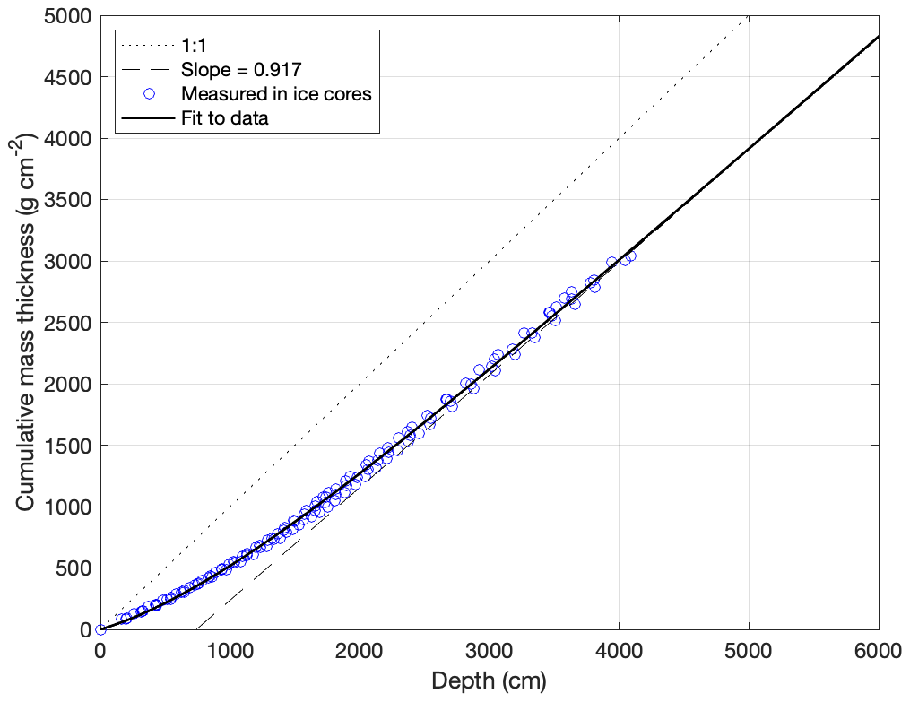
Figure 8 Relationship between linear thickness and mass thickness for ice and firn at Kay Peak core sites. Blue circles are observed cumulative mass thickness derived from downcore measurements of firn and ice density at all core sites. The solid black line is Eq. (1) with fitted values of D and L.

Cosmogenic-nuclide production rates P(H,z) (atoms g⁻¹ yr⁻¹) are calculated from surface elevation H(t) and mass thickness z(t) as the sum of near-surface production by high-energy neutron spallation and production by deeply penetrating muons. Spallogenic production is exponential with an attenuation length of 140 g cm⁻² (Balco, 2017). Surface production rates due to spallation use the scaling method of Stone (2000) and the Antarctic atmosphere approximation of Radok et al. (1996), as implemented by Balco et al. (2008). Spallogenic ¹⁰Be and ²⁶Al production is calibrated using the “primary” calibration data set of Borchers et al. (2016). Spallogenic ¹⁴C production is calibrated from measurements at Tulane of the ¹⁴C concentration in the CRONUS-A intercomparison standard (Jull et al., 2015), which was collected from a site in the Antarctic Dry Valleys, and the assumption of production–decay equilibrium at that sample site (Balco et al., 2019; Goehring et al., 2019; Nichols et al., 2019). Production rates due to muons use Model 1A of Balco (2017) with cross-sections for ¹⁰Be, ²⁶Al, and ¹⁴C production as calibrated in that reference. Given the production rate P(H(t),z(t)), the nuclide concentration at the present time is the integral:

$$\begin{array}{}\text{(2)}& N=\underset{\mathrm{0}}{\overset{t_{\max }}{\int }}P\left(H\right(t),z(t)+z_{\mathrm{s}})e^{-\mathit{\lambda }t}\mathrm{d}t,\end{array}$$

where z_s is the mass depth of a core sample below the bedrock surface (g cm⁻²) and λ is the decay constant (year) for the nuclide in question. Samples are assumed to have a zero nuclide concentration at the beginning of the elevation change history (t=t_max). For computational efficiency, P(H,z) is precalculated on a 2 d mesh in H and z and is used as a lookup table during integration. Interpolation in z is log-linear to improve accuracy. We used the default numerical integration routine provided by MATLAB numerical computation software.

The random search algorithm generates piecewise-linear age–elevation histories H(t) that are constrained by geological and geochronological observations, applies the forward model for cosmogenic-nuclide production to compute predicted nuclide concentrations in the core samples corresponding to the age–elevation history, and then compares predicted to observed concentrations to identify H(t) that fit the observations. The randomly generated age–elevation histories have the following properties. First, the ice surface is at 350 m elevation between 35 ka and the Early Holocene (Johnson et al., 2020). An elevation of 350 m is chosen because it is slightly above the elevation of the highest glacial erratics with post-LGM exposure ages found on Kay Peak Ridge (Johnson et al., 2020). The LGM surface may have been higher, but the exact value chosen is not significant in this calculation because cosmogenic-nuclide production rates under >100 m of ice are insignificant in our calculation. Second, the beginning of deglaciation is drawn from a uniform random distribution between 9 and 6 ka. These limits are selected to be consistent with regional exposure-age data (Johnson et al., 2020; Adams et al., 2022). Third, the elevation change history after initial deglaciation consists of three piecewise-linear segments between the beginning of deglaciation and the present time. These are generated by selecting two times from a uniform random distribution within this interval as well as two surface elevations from a uniform random distribution between the elevation of the top of sediment-rich ice at a core site (0.7–1.2 m above the bedrock surface) and 100 m elevation (20–25 m above bedrock at the core sites). The 100 m upper limit was chosen after initial experiments to exclude regions of the parameter space that would be certain to yield poor fits to the data, thus improving the efficiency of the random search algorithm. Constraining the minimum thickness to be the thickness of sediment-rich ice observed at present is based on the assumption that the dirty basal ice is the result of subglacial erosion at the LGM and that if the ice had been thinner following the LGM, this unit would no longer be present. Fourth, the ice at the core site reaches its present (2019–2020) elevation at t=0. Omitting post-1966 thinning to simplify this constraint does not have a significant effect on the results. Finally, following the reasoning in the previous section, subglacial erosion during the Holocene is assumed to be zero. Note that the assumption that nuclide concentrations are zero at t=t_max means that it is not necessary to specify subglacial erosion during LGM conditions. Alternatively, the zero initial condition assumption could be considered an assumption that meter-scale erosion did take place during the LGM.

We quantify the fit of predicted to observed ¹⁰Be and ¹⁴C concentrations in cores using an error-weighted sum-of-squares statistic M:

$$\begin{array}{}\text{(3)}& M={\displaystyle \frac{\mathrm{1}}{n}}\sum _{i=\mathrm{1}}^n{\left[{\displaystyle \frac{(N_{\mathrm{m},i}-N_{\mathrm{p},i})}{\mathit{\sigma }{N}_{\mathrm{m},i}}}\right]}^{\mathrm{2}},\end{array}$$

where N_m,i is the measured nuclide concentration (atoms g⁻¹) in analysis i, N_p,i is the nuclide concentration predicted by the forward model for the sample on which analysis i was made, and σN_m,i is the uncertainty in the measured nuclide concentration. This formulation implies a normal uncertainty distribution for N_m,i. As this is not the case for the ¹⁴C measurements (Methods 2 in the Supplement), we approximate the uncertainty distribution for ¹⁴C measurements as an asymmetrical normal distribution with different values of σN_m,i above and below. Because ²⁶Al measurements were only made in one core (19-KP-H1), we use only ¹⁰Be and ¹⁴C data in computing M, thereby standardizing the calculation for all cores. However, as discussed below, ²⁶Al data are exactly consistent with the ¹⁰Be measurements, so including or excluding them in calculating M for core 19-KP-H1 does not affect the results. If we assume that all measurement uncertainties are correctly characterized, the model correctly represents all operative processes, and predicted and observed values differ only due to measurement uncertainties, then the expected value of M is near 1. However, these assumptions are not completely correct. For example, we have disregarded uncertainty in production rates due to muon interactions, which may be 10 % or greater (this was omitted because production rate uncertainties are correlated between core samples, which complicates interpretation of a misfit statistic). Thus, we view minimum values of M near 2 generated by the random search algorithm as acceptable fits. All results of the random search algorithm are shown in Methods 3 in the Supplement.

Ice thickness change histories generated by the random search algorithm that fit the bedrock core data uniformly include a period of several thousand years during which the ice was several meters thick at the core sites (Figs. 9 and 7 as well as Methods 3 in the Supplement). Ice thickness during this lowstand is in the range of 2–5, 3–6, and 4–7 m at 19-KP-H1, 19-KP-H4, and 19-KP-H5, respectively, implying 30–35 m of thinning relative to present. Although we only assessed the model fit against data from the bedrock cores and not against the exposure-age data from the exposed ridge, scenarios that fit the subsurface data follow the older bound of the surface data, which is consistent with the hypothesis that scatter in these data is the result of locally derived snow and ice fields that persisted after ice surface lowering. Scenarios with shorter lowstands, or thicker ice during the lowstands, predict systematically lower cosmogenic-nuclide concentrations than observed (Fig. 7).

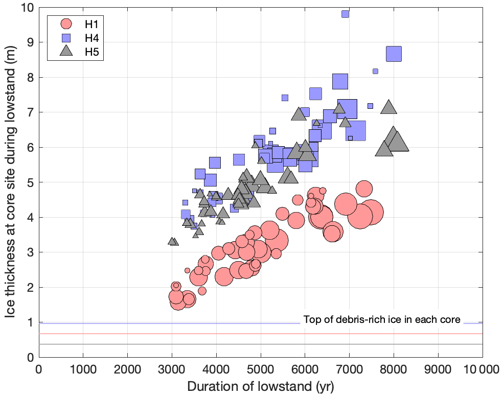
Figure 9 Trade-off between lowstand duration and ice thickness during lowstand in fitting measured ¹⁰Be and ¹⁴C concentrations. This shows the 50 (out of 2000) best-fitting iterations of the random search algorithm applied to each core, where the ice thickness history in each iteration is simplified by representation as the duration of a Late Holocene ice thickness minimum and the mean ice thickness during that period. Relatively long lowstands with relatively thick ice fit the observations similarly to relatively short lowstands with relatively thin ice. The size of the symbols reflects goodness of fit: scenarios represented by larger symbols have lower values of M. For best readability, the symbol size is scaled to the respective range of M in each core. This highlights that scenarios with longer lowstand durations are slightly, but not strongly, favored. This figure also shows that ice thickness histories that fit data from each core are systematically offset: regardless of the duration of the lowstand, ice covering H1 is required to be ∼2 m thinner during the lowstand than ice covering H4 and H5.

Ice thickness change histories that fit the measured nuclide concentrations display a trade-off between lowstand duration and ice thickness during the lowstand. A longer lowstand duration predicts higher nuclide concentrations, and thicker ice during the lowstand predicts lower nuclide concentrations. A longer-duration lowstand with thicker ice therefore yields a similar fit to data as a shorter-duration lowstand with thinner ice during the lowstand. Thus, it is not possible to choose a single best-fitting thickness change history or to accurately date the beginning and end of the lowstand. For example, a 4000-year period with 3 m thick ice fits the data for core H1 as well as a 7000-year period with 5 m thick ice (Fig. 9.). However, all cores require a lowstand period of no less than 3000 years during which ice was no thicker than several meters (Figs. 7, 9).

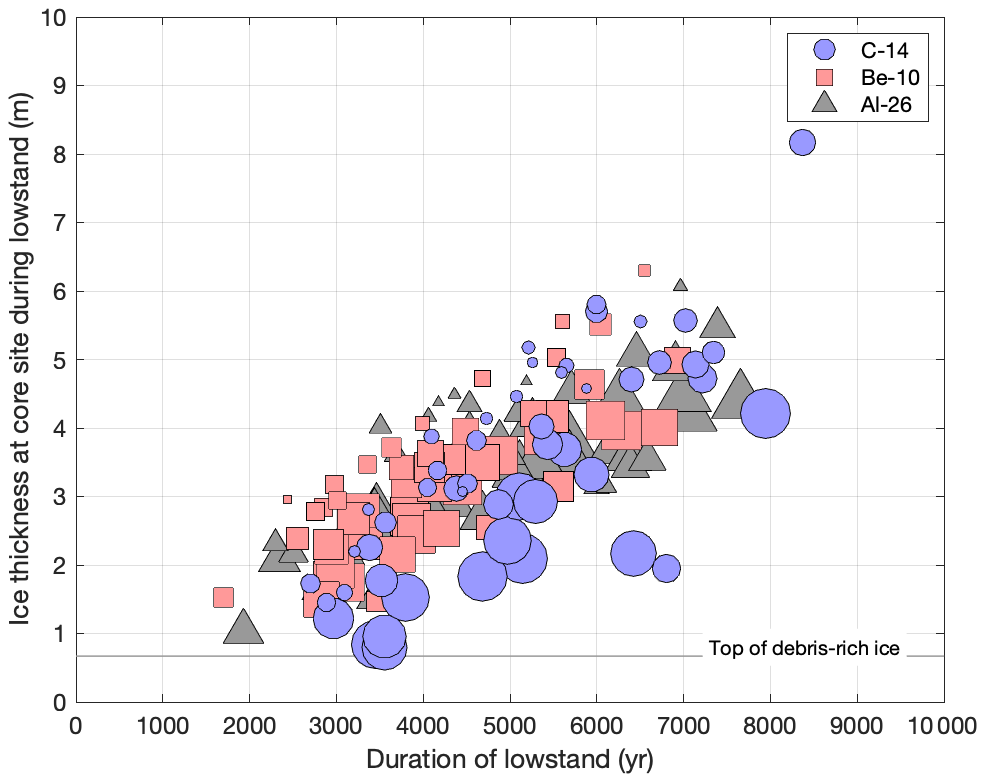
Figure 10 Elevation change histories that fit ¹⁰Be, ²⁶Al, and ¹⁴C data sets, considered separately, for core 19-KP-H1. As in Fig. 9, each elevation change history is represented by a lowstand duration and a mean ice thickness during the lowstand. The best-fitting 50 (out of 1000) results are shown for each nuclide, and, following Fig. 9, the symbol size is proportional to goodness of fit. Fitting to ¹⁰Be and ²⁶Al measurements separately yields identical results. Although a wider range of lowstand thicknesses are permitted by the ¹⁴C data because they have larger measurement uncertainties and therefore more scatter, concentrations of all three nuclides require a lowstand of similar magnitude and duration.

Finally, the fact that the same Late Holocene lowstand scenarios are inferred from fitting ¹⁰Be, ¹⁴C, and ²⁶Al measurements separately (Fig. 10) precludes the possibility that any significant fraction of the measured ¹⁰Be or ²⁶Al inventory was inherited from pre-Holocene exposure, perhaps in an interglacial period prior to the LGM. If this were the case, corresponding inherited ¹⁴C would have been removed by radioactive decay, and a longer period of exposure would be required to fit the ¹⁰Be and ²⁶Al data than the ¹⁴C data. Subglacial erosion during the last glacial cycle, as also suggested by the presence of debris-rich basal ice and IRSL data precluding sunlight exposure in the last 200–300 ka, likely removed rock surfaces exposed during prior interglaciations.

To summarize, although IRSL data show that bedrock at the core sites was not ice-free in the Holocene, the cosmogenic-nuclide data show that ice at the core sites was 30–35 m thinner than present for at least 3000 years, and possibly as long as 8000 years, during the Middle to Late Holocene. The coincidence of IRSL data that preclude direct exposure of rock surfaces to sunlight and cosmogenic-nuclide data that require significant ice thinning is consistent with the present geometry of ice and rock on the exposed portion of Kay Peak Ridge. Locating the ridge axis using single-channel ice-penetrating radar, as we did, is not expected to be precise at the meter scale because of limits on instrument resolution and the likelihood of off-axis reflections from irregular bedrock topography. The currently exposed portion of the ridge is mantled by ice fields on both sides that extend to within meters of the ridge axis and thicken with distance from the axis (Fig. 2). In addition, lowstand ice thicknesses inferred from the random search algorithm vary between cores over a range of 2–3 m (Fig. 9), but the core top elevations vary over a range of 6 m. These observations suggest that ice with a thickness of several meters present during the lowstand does not reflect a flat ice surface uniformly 35 m below the present surface but instead reflects a condition like what we observe now, in which fringing ice fields of varying thickness covered drill sites that are slightly off the ridge axis. This, in turn, indicates that the estimate of 35 m of thinning is a minimum. Areas farther from the ridge axis nearly certainly thinned more.

6 Summary and conclusions

Our subglacial bedrock exposure-dating results are direct, unambiguous evidence for ice thinning and subsequent thickening of at least 35 m during the past several thousand years. Ice thinning below present conditions earlier in the Holocene was not followed by further runaway thinning and significant regional ice loss. Instead, it was followed by thickening to the present ice sheet configuration. The significance of this observation with respect to the question of whether or not grounding line retreat and thinning observed in recent decades is or is not irreversible depends on whether or not the ice thickness at Kay Peak is an accurate proxy for grounding line position. If one accepts that simultaneous thinning at Kay Peak and retreat of the Pope Glacier grounding line observed in recent decades are dynamically linked, then our observation that mid-Holocene thinning below the present ice thickness was reversible implies that mid-Holocene grounding line retreat inboard of present positions was also reversible. By analogy with present conditions, thinning and subsequent thickening of 35 m or more may have been associated with grounding line retreat tens of kilometers upstream of present locations, and subsequent readvance.

These observations, with independent evidence for falling relative sea level in the nearby Pine Island Bay region during the past 4000 years (Braddock et al., 2022), most likely indicate that a grounding line retreat–advance cycle driven by glacioisostatic rebound–RSL feedback took place during the Holocene. Observations from elsewhere in Antarctica (Bradley et al., 2015; Kingslake et al., 2018; Venturelli et al., 2020; King et al., 2022; Johnson et al., 2022) indicate that this likely took place at many marine ice margins around the continent. In general terms, therefore, our results provide supporting evidence for the hypothesis that glacioisostatic rebound can provide an important stabilizing feedback on grounding line retreat. However, boundary conditions during a Late Holocene retreat–readvance cycle were not identical to present conditions. Applying evidence for a Holocene retreat–readvance cycle to determine the importance of glacioisostatic rebound feedback in stabilizing present grounding line retreat in the Amundsen Sea region also requires understanding the following: (i) the difference between isostatic responses to large-scale LGM-to-Holocene thinning that took place over thousands of years and thinning of lesser magnitude observed in recent decades; (ii) the relative importance (to the grounding line position) of relative sea level change, ice shelf buttressing, and sub-ice-shelf melting driven by oceanographic conditions, which cannot be deduced from any data presented here; and (iii) past and present bed topography in the region of grounding lines. In addition, the past thinning–thickening cycle that we have detected spanned a duration of at least 3000 years, which is geologically rapid but slow by comparison to the timescale of projected sea level rise impacts of present ice sheet thinning.