Climatic control on seasonal variations in mountain glacier surface velocity

Accurate measurements of ice flow are essential to predict future changes in glaciers and ice caps. Glacier displacement can in principle be measured on the large scale by cross-correlation of satellite images. At weekly to monthly scales, the expected displacement is often of the same order as the noise for the commonly used satellite images, complicating the retrieval of accurate glacier velocity. Assessments of velocity changes on short timescales and over complex areas such as mountain ranges are therefore still lacking but are essential to better understand how glacier dynamics are driven by internal and external factors. In this study, we take advantage of the wide availability and redundancy of satellite imagery over the western Pamirs to retrieve glacier velocity changes over 10 d intervals for 7 years and for a wide range of glacier geometry and dynamics. Our results reveal strong seasonal trends. In spring/summer, we observe velocity increases of up to 300 % compared to a slow winter period. These accelerations clearly migrate upglacier throughout the melt season, which we link to changes in subglacial hydrology efficiency. In autumn, we observe glacier accelerations that have rarely been observed before. These episodes are primarily confined to the upper ablation zone with a clear downglacier migration. We suggest that they result from glacier instabilities caused by sudden subglacial pressurization in response to (1) supraglacial pond drainage and/or (2) gradual closure of the hydrological system. Our 10 d resolved measurements allow us to characterize the short-term response of glaciers to changing meteorological and climatic conditions.

1 Introduction

Glaciers and ice caps are shrinking around the world in response to current global warming caused by human activities (IPCC, 2021). Projecting their future change is critical to assess the associated impacts in terms of sea-level rise, naturals hazards and water resources (Azam et al., 2021). Such projections rely on our ability to observe and understand glaciological processes at various temporal and spatial scales. A key manifestation of glacier dynamics is surface velocity (hereinafter referred to as “velocity” for brevity), which depends on both internal (e.g., glacier geometry, bed types) and external (e.g., air temperature, precipitation) factors. Although field-based measurements can provide very accurate data about glacier processes (e.g., Stevens et al., 2022; Nanni et al., 2022; Vincent et al., 2022), they require human presence and are generally limited to accessible areas, resulting in poor spatial and temporal coverage. In contrast, satellite imagery provides wide spatial coverage and is therefore an effective approach for retrieving glacier-flow characteristics in remote areas and on a large or even global scale (Li et al., 1998; Berthier et al., 2005; Scherler et al., 2008; Rignot et al., 2011; Dehecq et al., 2015, 2019; Gardner et al., 2019; Millan et al., 2022).

When using satellite imagery to study glacier flow, cross-correlation techniques are often used to track the movement of features on the glacier surface (Scambos et al., 1992; Strozzi et al., 2002; Kääb et al., 2002; Leprince et al., 2008; Heid and Kääb, 2012). Obtaining an accurate glacier velocity depends on the ability to obtain a high signal-to-noise ratio (SNR) for the expected glacier displacement (meters to kilometers per year). The SNR depends on the methods chosen and the quality of the images (e.g., resolution, georeferencing, orthorectification) used for cross-correlation (Heid and Kääb, 2012; Millan et al., 2019). The time interval between optical images that are correlated is an important parameter, as a larger time interval will increase the signal (i.e., the displacement) relative to the noise of the measurement. Annual to multi-year time periods allow expected displacements to be large relative to the noise, so that automated procedures can effectively recover accurate velocity variations on global (e.g., ice sheets, mountain ranges) and local (e.g., a small mountain glacier) scales (Quincey et al., 2009; Rignot et al., 2011; Scherler et al., 2011; Dehecq et al., 2015; Mouginot et al., 2017)

These observations, when coupled with appropriate modeling and complementary datasets (e.g., ice thickness), allow the monitoring of surface-mass balance changes over long periods (several years) and assessing the glacier response to climate change (Tedstone et al., 2013; Kjeldsen et al., 2015; Dehecq et al., 2019). On seasonal timescales, velocity variations have been documented on outlet glaciers and large mountain glaciers, where displacements are large enough to be well above the noise level (Scherler and Strecker, 2012; Armstrong et al., 2017; Altena and Kääb, 2017; Usman and Furuya, 2018; Derkacheva et al., 2020; Riel et al., 2021; Yang et al., 2022; Beaud et al., 2022). Various processes are responsible for seasonal variations in glacier dynamics as well as glacier surges and flow instabilities and probably result from hydrological controls (Tedstone et al., 2013; Moon et al., 2014; Quincey et al., 2015; Stearns and Van Der Veen, 2018; Derkacheva et al., 2021; Bouchayer et al., 2022). On shorter timescales (weeks to months), the expected displacement is often on the same order as the noise for commonly used satellite imagery (Millan et al., 2019), which limits the retrieval of accurate glacier velocities. Most studies that have looked at changes in glacier flow between weeks and months tend to focus on individual glaciers (Scherler and Strecker, 2012; Armstrong et al., 2016; Derkacheva et al., 2020; Riel et al., 2021; Beaud et al., 2022), and only a few studies have conducted such investigations over larger areas (Altena et al., 2019; Yang et al., 2022), demonstrating the opportunity to better understand how glacier dynamics (e.g., basal sliding) and glacier instability are affected by climatic conditions (Tedstone et al., 2013; Stearns and Van Der Veen, 2018; Kääb et al., 2018; Beaud et al., 2022).

Systematic acquisition planning and new generations of medium-resolution, short-recurrence-time optical sensors, such as Landsat 8 (15 m resolution in the panchromatic band, maximum 16 d recurrence time; operational since 2013) and Sentinel-2 (10 m resolution in the visible bands, maximum 5 d recurrence time; operational since 2016), have fostered new methodological developments to measure glacier velocity variations on relatively short (< month) timescales (Armstrong et al., 2017; Altena et al., 2019; Derkacheva et al., 2020; Riel et al., 2021). When using these medium-resolution images, it is crucial to preserve the true signal while removing poor correlations during post-processing, preferably in an automated manner to be applied over large areas. Recent studies have proposed efficient and accurate use of the large database of available satellite imagery to retrieve accurate short-term changes in glacier velocity (Altena et al., 2019; Derkacheva et al., 2020; Riel et al., 2021; Hippert-Ferrer et al., 2020). However, most of these studies have focused on fast outlet glaciers (Derkacheva et al., 2020; Riel et al., 2021) or other fast glaciers with large monthly-scale velocity changes (Altena et al., 2019; Millan et al., 2019; Hippert-Ferrer et al., 2020). It is not yet clear whether these approaches can be used to study the short-term dynamics of mountain glaciers in general or only for some of the largest and fastest glaciers. Large-scale assessments of velocity changes on short timescales and over complex areas such as mountain ranges are therefore still lacking.

In this study, we examine short-term (weekly to monthly) changes in glacier velocity in the western Pamirs, a mountain range that hosts a wide variety of glaciers in terms of geometry and dynamics. Our study aims to assess the temporal and spatial extent to which significant changes in glacier velocity can be retrieved using the latest generation of optical sensors with global coverage. We first present a semi-automated processing protocol designed to examine changes in velocity on weekly to monthly timescales over entire mountain ranges. We then apply our methodology in the western Pamir region to investigate its performance, as this region features glaciers with different characteristics (e.g., velocities) and geometries (e.g., glacier length) as well as low cloud cover, compared to other regions such as the Karakoram or the Alaskan Range. We finish by discussing the observed velocity variations and the ability of our approach to provide information on the interactions between climatic conditions and glacier dynamics.

2 Study site

The western Pamirs in Tajikistan (Fig. 1) is characterized by high peaks, steep slopes and deep narrow valleys that are home to abundant mountain glaciers, of which the 72 km long Fedchenko Glacier is the largest mountain glacier outside the polar regions. The regional equilibrium line altitude (ELA) lies between 4600 and 4800 m above sea level (a.s.l.) (Aizen, 2011). Average glacier velocities have been stable in this region since 2008, and the glaciers have been interpreted to be close to equilibrium by Dehecq et al. (2019). The climate is characterized by westerly-controlled snowfall during winter and warm and dry summers (Yao et al., 2012). Long-term temperature measurements at the Goburnov station (elevation of 4200 m, close to the Fedchenko Glacier) show positive daily mean air temperatures from late May to early October (Lambrecht et al., 2014, 2018; Fig. S1 in the Supplement). We focus our study on seasonal variations in glacier velocity that repeat from year to year and do not investigate surges or inter-annual dynamics.

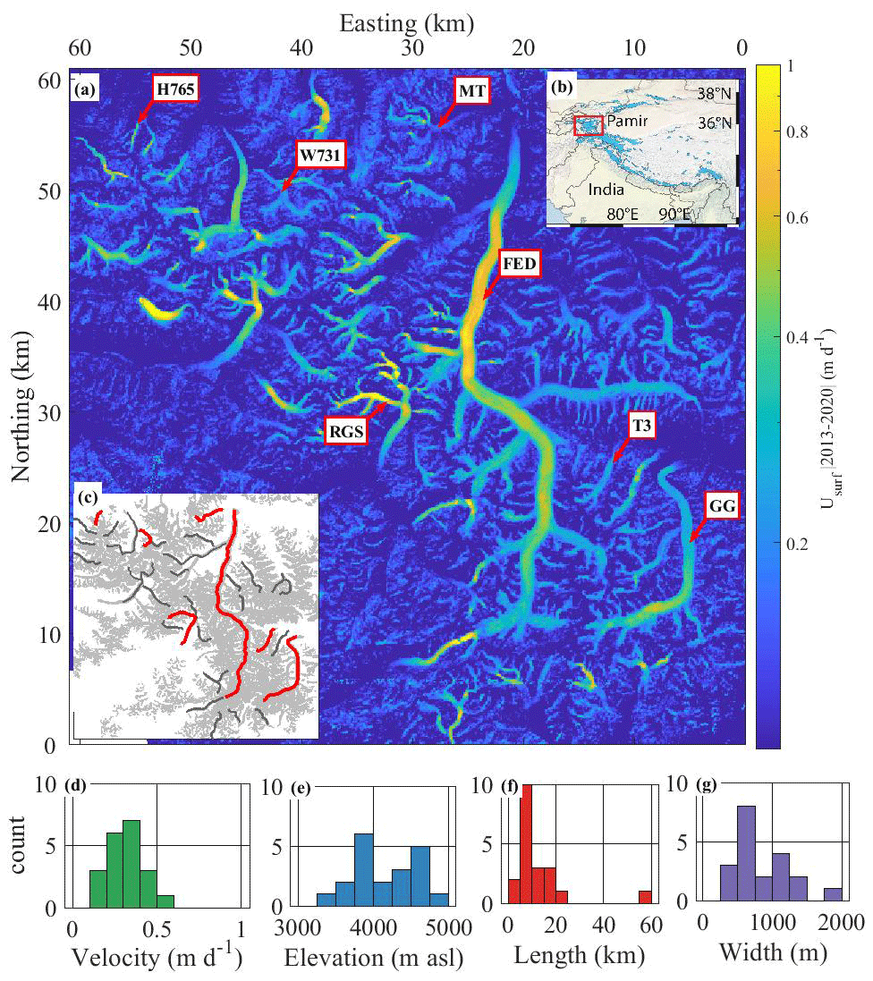
Figure 1 (a) Glacier velocity (m d⁻¹) mosaic of the western Pamir mountain range, averaged (median) over the time period 2013–2020. Velocity is obtained at a horizontal resolution of 40 m using 650 pairs of Sentinel-2 images and 400 pairs of Landsat 8 images (see the “Materials and methods” section for details). Color bar is coded on a logarithmic scale going from blue (no displacement) to yellow (fast displacement). Text boxes show the names (based on Randolph Glacier Inventory, 2017) of the seven glaciers investigated in detail: the Fedchenko Glacier (FED); the Tanymas 3 Glacier (T3); the Grumm-Grzhimaylo Glacier (GG); the Russian Geographical Society Glacier (RGS); the Walter 731 Glacier (W731); the Hadyrsha 765 Glacier (H765); Malyy Tanymas Glacier (MT). All of these glaciers flow northward, except for RGS, which flows southward. (b) Location of the western Pamirs in the regional context; blue areas show glacier coverage (Randolph Glacier Inventory, 2017); background shaded relief provided by ASTER (2019). (c) Glaciated area (gray), flowlines (red) of the seven glaciers previously mentioned and the flowlines (dark gray) of 31 additional glaciers investigated. (d, e, f, g) Characteristics of the studied 38 glaciers, in terms of median velocity, median elevation, length and median width. Easting and northing are relative to 38.39^∘ N, 72.63^∘ E in the UTM 32N projection.

Our study is focused on a 60 km × 60 km area that is approximately centered on the Fedchenko Glacier. We selected 38 out of 48 studied glaciers for further analysis based on the presence of clear seasonal variations and limited surge occurrence (lines in Fig. 1c). This selection contains a wide range of glacier geometries (see Fig. 1 caption for abbreviations): from small (< 5 km long) and narrow (< 500 m wide; e.g., the Hadyrsha 765 Glacier, H765) to mid-sized (e.g., the Russian Geographical Society Glacier, RGS) and very large glaciers (> 20 km long), such as the Grumm-Grzhimaylo Glacier (GG) and the Fedchenko Glacier (FED) (Fig. 1 d to g).

3 Materials and methods

3.1 Image selection and cross-correlation

We downloaded Landsat 8 and Sentinel-2 images that cover our study area for the time period 2013–2020 from USGS EarthExplorer (https://earthexplorer.usgs.gov/, last access: 9 September 2022) and the Copernicus Open Access Hub (https://scihub.copernicus.eu, last access: 9 September 2022), respectively. As we are interested in short-term changes in glacier velocity, we correlated images that are separated by 16 and 32 d for Landsat 8 and by 10, 20 and 30 d for Sentinel-2. These repeat cycles provide good temporal coverage while maintaining sufficient accuracy for measuring the expected glacier velocities in our region (Lambrecht et al., 2014; Millan et al., 2019). To minimize residual stereoscopic effects, we only correlated image pairs from the same sensor and tile (see Fig. S2 for the number of correlations per cycle and sensor). We used panchromatic band (B8, 15 m spatial resolution) imagery of the USGS/NASA Landsat 8 dataset for the years 2013–2020 and band 8 (10 m spatial resolution) imagery of the Copernicus Sentinel-2 dataset for the years 2017–2020, as its availability in this area started in 2017 (Figs. S2, S3 and S4 in the supporting information). These images are georeferenced and orthorectified with quality assessment bands (for Landsat 8), which contain information on surface, atmospheric and sensor conditions. Glacier contours provided by the Randolph Glacier Inventory (2017) are used to distinguish between glaciers and stable ground.

The displacement that occurs between the acquisition of two images is measured using ENVI's COSI-Corr add-on software (freely available at http://www.tectonics.caltech.edu/slip_history/spot_coseis/, last access: 9 September 2022). We used a frequency correlation with a search window size (w) that ranged from 64×64 to 32×32 pixels. Note that by apodizing with a 2D Hanning function, the spatial resolution is better than the correlation window size (Leprince et al., 2007). This technique had already been used on mountain glaciers and yielded a stated 1σ uncertainty of about $\mathrm{1}/\mathrm{10}$ of the pixel size (Scherler et al., 2008; Herman et al., 2011). The displacement is calculated in steps (s) of four pixels in the x and y directions, resulting in a displacement ground sampling distance of 60 m for Landsat 8 and 40 m for Sentinel-2. Steps smaller than the search window size allow for measurement redundancy (Leprince et al., 2008), which increases its accuracy compared to steps that are similar to the search window (Fahnestock et al., 2016). The output of COSI-Corr consists of three images: the east–west (EW) and north–south (NS) components of the displacement and the associated signal-to-noise ratio (SNR), which assesses the quality of the correlation at each pixel. The results of all correlations are combined into a single data cube for each sensor before applying our post-processing procedure.

3.2 Basic filtering

We applied a basic filtering procedure to the NS and EW components of each surface displacement that does not depend on the calculated total displacement. We started by setting a threshold for the signal-to-noise ratio (SNR ≥0.97) to exclude poor correlation results (Scherler et al., 2008). In addition, we used the quality assessment band for Landsat 8 images to flag and remove pixels, where clouds, including cirrus, are present in either one of the correlated images. After calculating the total displacement amplitude (hereinafter referred to as the velocity), we removed pixels associated with unrealistically high-velocity values that exceed a threshold value of 15 m d⁻¹ (5475 m yr⁻¹). The chosen value of this threshold was guided by previous estimates of annual glacier velocities (Dehecq et al., 2015) but set sufficiently high to allow for physically meaningful variations. Finally, to avoid edge effects, we removed a band as wide as the correlation window size from the edge of the image in all displacement maps.

3.3 Advanced filtering

3.3.1 Temporal redundancy of the velocity

We calculated the median magnitude of the NS and EW components (NS_med, EW_med) of the velocity and the associated median absolute deviation (MAD) and then removed all pixels where $\left|\mathrm{NS}-{\mathrm{NS}}_{\mathrm{med}}\right|>\mathrm{10}\cdot {\mathrm{NS}}_{\mathrm{MAD}}$, or $\left|\mathrm{EW}-{\mathrm{EW}}_{\mathrm{med}}\right|>\mathrm{10}\cdot {\mathrm{EW}}_{\mathrm{MAD}}$. This threshold is defined based on previous estimates of annual glacier velocities in the area (e.g., Dehecq et al., 2015). In doing so, we assume temporal coherence of the glacier velocity over time, which has the advantage of eliminating potential miscorrelations (Scherler et al., 2008) but at the risk of eliminating episodes during which glacier velocity changes dramatically. Our choice of threshold is motivated by the fact that we focus on short-term changes in glacier velocity rather than surge events, although the above filter can be easily adjusted to avoid exclusion of surge events. Our approach is simpler than the ones proposed by Derkacheva et al. (2020) and Riel et al. (2021), in which velocity time series are interpolated and filtered with multiple local regressions.

3.3.2 Spatial redundancy of the velocity

We assessed the validity of the measurement at each pixel by examining the similarity with neighboring values in a search area centered on the pixel in question. The measurement redundancy due to correlation depends on the window size w and the correlation step s and has a size of $\frac{\mathrm{2}w}{s}$ pixels (Leprince et al., 2007). This redundancy represents the distance to be covered to observe an independently recorded displacement. The search area is defined as a centered square with a half-length of $\mathrm{1}+\frac{\mathrm{2}w}{s}$ pixels, which means that half of the pixels are expected to have the same value within this square. Each pixel for which the surrounding square does not have at least half of its values similar (within 1 standard deviation) to that of the queried pixel is removed, both for the EW and NS components. This filtering procedure is similar to a spatial median filtering but based solely on the characteristics of the COSI-Corr correlation process, and it does not make any assumptions about the glacier flow (Leprince et al., 2007).

3.4 Calibration and stable ground correction

We further applied a filter to remove the bias introduced by uncorrected satellite attitude variations during orthorectification. To do this, we used non-glacial areas as defined by the RGI (assuming they represent stable ground), calculated the average velocity in the along-track and across-track directions of the EW and NS velocity, and removed them from the corresponding velocity maps. This procedure follows that of the COSI-Corr “destriping” tool, which has been shown to improve the accuracy of velocity measurements (Scherler et al., 2008). We then estimated the remaining bias from the distribution of the velocity measured over the non-glacial areas. We fitted the distribution of these measurements with a Gaussian curve using the least squares criterion and subtracted the Gaussian mean for each individual pair so that the distributions of the EW and NS velocity values were centered on 0. Finally, we removed isolated measurements, i.e., pixels surrounded by less than three non-zero values.

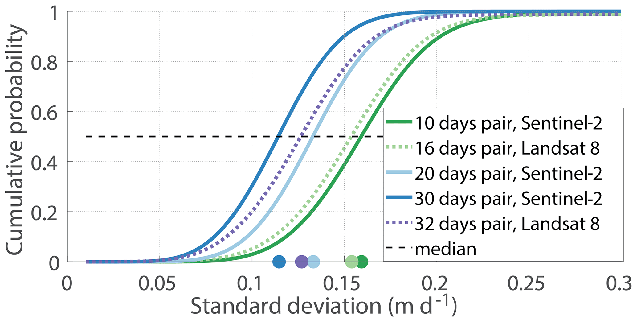
Figure 2 Cumulative distribution of the standard deviation of velocity in ice-free areas as a function of repeat cycle length for Sentinel-2 and Landsat 8 data. Colored points show the median value of the distribution for each repeat cycle, which represents the nominal precision achieved for each cycle.

3.5 Measurement precision

To assess the capability of each sensor to map short-term changes in velocity, we calculated the cumulative distribution of the standard deviation of the velocity in ice-free areas for different repeat cycle lengths (Fig. 2). We did not use the standard deviation in glaciated areas, as it likely represents natural fluctuation in velocity rather than the sensor precision (Fig. 1). The distribution is calculated for each pixel and based on all measured velocities. We assume that the median value of the distribution represents the nominal precision achieved for each cycle. Such an analysis of the standard deviation has been shown to reliably quantify sensor precision in mountain areas (Millan et al., 2019). We observe that the precision of velocity measurements used in our study ranges from 0.11 to 0.16 m d⁻¹ and decreases, as expected, with time separation between two acquisitions. For Sentinel-2 we obtain a precision of 0.16, 0.13 and 0.11 m d⁻¹ for 10, 20 and 30 d cycles, respectively. For Landsat 8, we obtain a precision of 0.15 and 0.12 m d⁻¹ for 16 and 32 d cycles, respectively. Similar results were achieved in the study by Millan et al. (2019). Note that the nominal precision obtained for Landsat 8 and Sentinel-2 is very similar. Assuming that the nominal precision depends only on image correlation, we calculated the sub-pixel matching precision as $\frac{{\mathit{\sigma }}_{\mathrm{cycle}}c}{\mathrm{ps}}$, where σ_cycle is the standard deviation of a given cycle, c is the cycle length and ps the pixel size. We find a sub-pixel image matching precision of 0.15 and 0.33 pixels for a 10 d cycle with Sentinel-2 and for a 32 d cycle with Landsat 8 imagery, respectively.

3.6 Retrieving velocity variations along the glacier flowline

We calculated the velocity magnitude as the norm of the NS and EW components. We then calculated the median velocity over the entire time period at each pixel location and used the resulting map (Fig. 1) to define the central glacier flowline (here done manually). For each correlation result, we extracted the velocity profile along the flowline by taking the median value from a three by three pixel square. In order to calculate a regularized time series over the period 2013–2019, we defined a time grid with a temporal resolution of 20 d. We chose this resolution because it represents the average time between pairs over the study period (Fig. S4). For each 20 d time step, we searched for velocity maps where the center of the time range falls in the 20 d period and calculated the median value of all available velocity estimates from different sensors and repeat cycles. This median-based approach has proven to be statistically robust when the sampling of the time series is sufficiently dense (Derkacheva et al., 2021), which is the case in our study. We did not use a weighted-median approach as we found that it introduced more noise than a regular median, which could be due to the fact that our repeat cycles are of similar length (i.e., 10 to 32 d). In agreement with Dehecq et al. (2019) we did not observe any clear long-term trend in the velocities that we could correct for. Finally, we calculated a characteristic annual velocity pattern with a 10 d resolution for each glacier by averaging the flowline profiles over a year using the same approach as described above. The higher resolution is made possible by the large number of image pairs available for each 10 d time step (Fig. S4).

3.7 Terminology

In the following, we refer to changes in velocity with respect to the annual median velocity. We express these changes both in absolute values (m d⁻¹) and in relative values (%); i.e., a value of −10 % corresponds to a velocity 10 % below the median velocity. We use the term “acceleration” to refer to abrupt changes in the velocity pattern, when the glacier velocity increases – typically – by more than 35 %. Such accelerations can have different onset dates at different elevations. We then consider any period of the year in which the velocity is typically 35 % above (below) the annual median velocity, a time of faster (slower) velocities.

4 Results

We analyzed 48 glaciers in the western Pamirs, from which we selected 38 that show clear seasonal changes in velocity over the 7-year period investigated (Fig. 1c, red and dark gray flowlines). We first present a detailed analysis for a selection of seven of these glaciers, which we consider to be representative of different geometries and dynamics, and then we present results for the full selection.

4.1 Seasonal velocity variations in the Fedchenko Glacier

In Fig. 3a, we show the 20 d changes in the velocity relative to the multi-annual median velocity calculated along the Fedchenko Glacier flowline (Fig. 1, FED) from spring 2013 to winter 2020–2021. We observe repeating seasonal variations in glacier velocity of up to 1 m d⁻¹ (Fig. 3a), which correspond to changes of up to 150 % near the glacier front (Fig. 3c). Such changes are 2 to 3 times higher than those described in the study of Lambrecht et al. (2014). In the ablation area (< 40 km upglacier distance), we observe pronounced changes relative to the median velocity with negative changes (−0.2 to −0.4 m d⁻¹) towards the end of each year (September to December) and positive changes (+0.3 to +0.7 m d⁻¹) around the second quarter of each year (March to July). Seasonal variations in the accumulation area are less pronounced, partly because the SNR is lower, which is probably related to areas of slow velocity and low texture due to snow cover (Fig. 3b). These seasonal variations are observed throughout the 7 years (Fig. 3a) but are more accurately represented during 2018 and 2019, likely because of the combination of Landsat 8 and Sentinel-2 data.

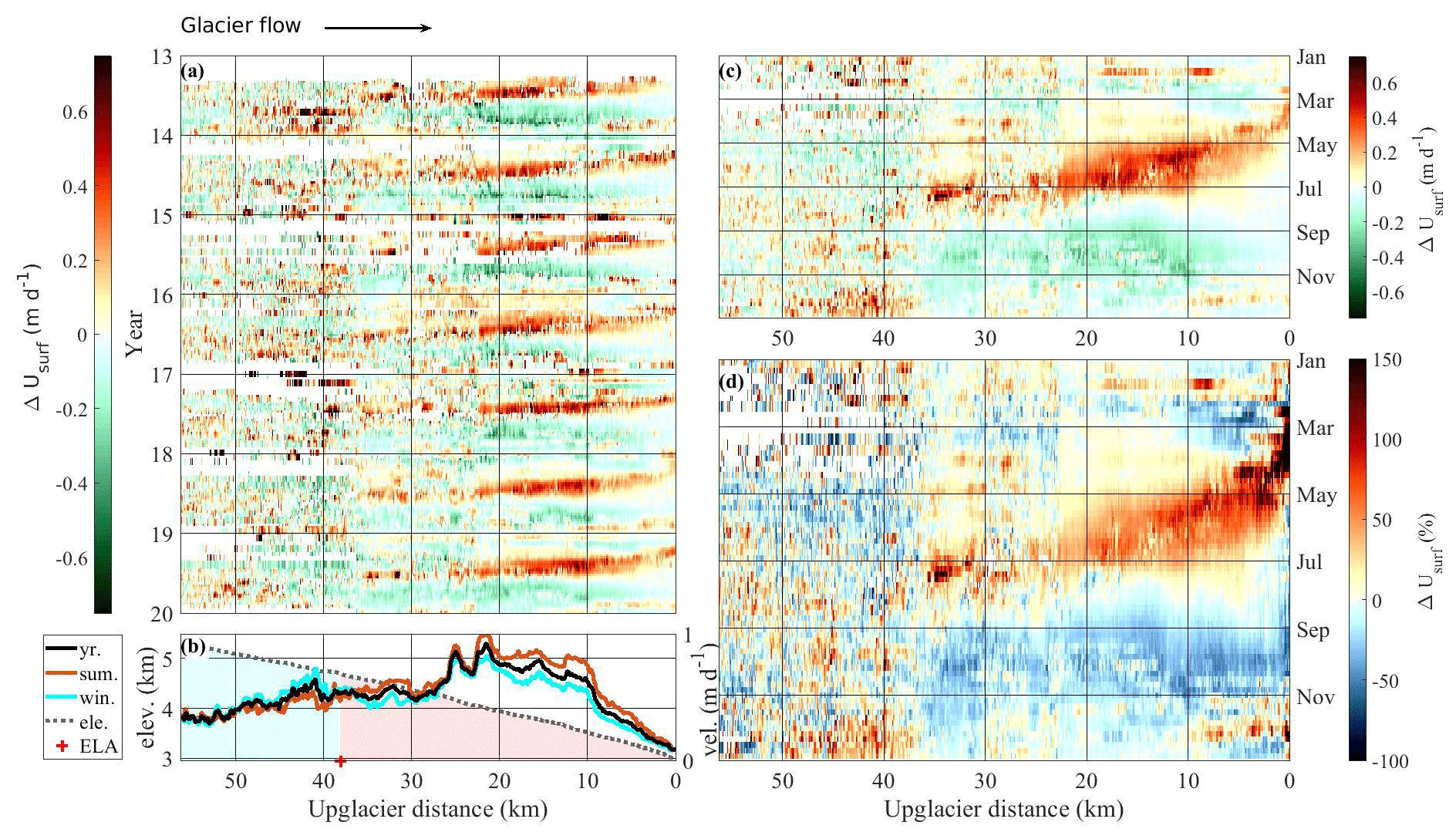
Figure 3 (a) Changes in glacier velocity relative to the multi-annual median velocity along the Fedchenko Glacier flowline averaged over 20 d and quantified using Sentinel-2 and Landsat 8 images. The color bar is coded on a linear scale from green (slower than the median velocity) to red (faster than the median velocity). The black arrow indicates the direction of glacier flow. (b) Seven-year median annual (black), summer (March to mid-August; brown) and winter (mid-August to February; cyan) velocity along the flowline (in m d⁻¹; right axis). Light gray line shows the elevation profile (in km; left axis), with the blue area located above the equilibrium line altitude (ELA) and the red area under the ELA. (c, d) Upglacier profile of characteristic annual absolute (c) and relative (d) changes in glacier velocity relative to the annual median velocity along the Fedchenko Glacier flowline, averaged over 10 d for each year. Changes in percent are evaluated relative to the median velocity; i.e., a change of −10 % corresponds to a velocity 10 % below the median velocity.

Stacking velocities of all individual years into a characteristic annual velocity time series removes some of the noise from individual years (Fig. 3c, d) and shows that the annual evolution of velocity changes follows a characteristic pattern, best described by an upglacier migration of glacier acceleration. At the end of February, the lowest part of the ablation zone (< 10 km upglacier distance), where the median velocity is about 0.25 m d⁻¹, accelerates by 0.3 m d⁻¹, i.e., by more than 100 %. Between April and May, the acceleration extends for about 10 km upglacier (45 km downglacier distance) with similar changes, and, simultaneously, the previously fast-flowing areas near the terminus start to slow down. By the end of June, the acceleration has migrated ca. 35 km upglacier, where the median velocity is about 0.5 m d⁻¹, reaching changes in velocity of more than +0.7 m d⁻¹, or +50 % to +150 %. In June and July, velocities in the upper part of the ablation zone (30–35 km upglacier distance), increased by 0.3 to 0.6 m d⁻¹ or 50 % to 100 %. Overall, the upglacier migration of this acceleration takes about 4 to 5 months. This acceleration is followed by a period of fast velocity lasting from 1 to 3 months over a given area of the glacier. In the following, we refer to this acceleration as the spring/summer acceleration. We observe that the area of fast velocity widens with time, which means that acceleration migrates up the glacier faster than the deceleration does. At the same time, it appears that the average acceleration becomes lower while moving upglacier, with acceleration above 100 % on a narrow section near the terminus (< 10 km upglacier distance) in April and acceleration of the order of 50 % in June–July further up the glacier. This period is then followed by slow velocities from August to October, when velocities are about 0.5 m d⁻¹ below the median velocity (range of −50 % to −75 %). Between November and December, we observe a short period of fast velocity over the lower part of the glacier (< 10 km upglacier distance) with an acceleration of up to 0.5 m d⁻¹, i.e., by 100 % to 150 %. This acceleration is well visible in the years 2018 and 2019 and also suggested in the years 2013 and 2016 (Fig. 3a). In the following, we refer to this second acceleration in the ablation zone as the autumn acceleration. In the next section, we show similar velocity patterns from other glaciers in the vicinity.

4.2 Similarities and differences in seasonal glacier velocity

In Fig. 4, we show the characteristic annual velocity time series along the flowline of each of the six selected glaciers (Fig. 1), based on velocity stacking from spring 2013 to winter 2019–2020. These glaciers cover a range of velocities, from rather slow (< 0.2 m d⁻¹) to fast (> 0.5 m d⁻¹), and a range of glacier sizes with glacier lengths from less than 5 km to 24 km. However, each velocity time series has its own particularity, which we describe below.

We observe a spring/summer acceleration for all six glaciers. Analogous to the Fedchenko Glacier, velocity changes are larger near the glacier front (> +100 %) than in the upper part (range of +25 % to +75 %), except for the Malyy Tanymas Glacier (MT) (Fig. 4j), which shows fast velocities ($\sim +\mathrm{150}$ %) along its entire length. The accelerations do not start at the same time for all glaciers, with an onset in early March for RGS (Fig. 4e, g) and MT (Fig. 4j, l) and a later onset in May to early June for T3 (Fig. 4a, c) and H765 (Fig. 4i, k). Furthermore, the accelerations affect the whole length of RGS (Fig. 4e), the Walter 731 Glacier (W731; Fig. 4f), H765 (Fig. 4i) and MT (Fig. 4j). For T3 (Fig. 4a) and GG (Fig. 4b), the accelerations are limited to the lower part, as for the Fedchenko Glacier. We note that these three glaciers reach higher altitudes than the four others (see associated elevation profiles in Figs. 3c and 4c, d). The upglacier migration of the acceleration is visible well on three of the six glaciers (Fig. 4a, i, j), which shows that such velocity variations can be observed both on large (e.g., the Fedchenko Glacier) and very small glaciers (e.g., H765 and MT).

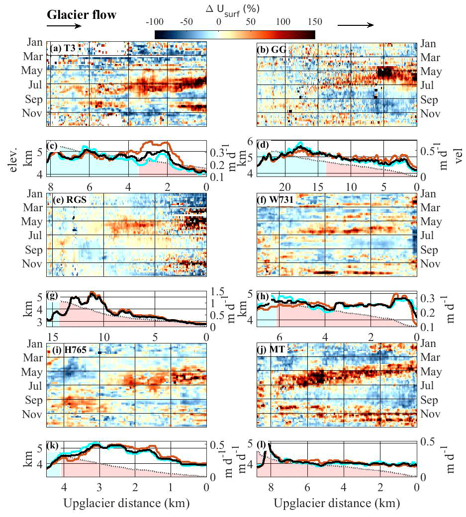
Figure 4 Annual pattern of glacier velocity changes relative to the annual median velocity along the flowline of the selected glaciers in Fig. 1a (green lines; except for the Fedchenko Glacier). Changes are expressed in percent to the annual median velocity for panels (a), (b), (e), (f), (i) and (j). (a, c) Tanymas 3 Glacier; (b, d) Grumm-Grzhimaylo Glacier; (e, g) Russian Geographical Society Glacier; (f, h) Walter 731 Glacier; (i, k) Hadyrsha 765 Glacier; (j, l) Malyy Tanymas Glacier. The 7-year median annual (black), summer (brown) and winter (cyan) velocity along the flowline is shown below each glacier (in m d⁻¹; right axis). Glaciers flow from left to right (black arrow). Light gray line shows the elevation profile (in km; left axis), with the blue area located above the ELA and the red area under the ELA. The color bar is the same for all glaciers. It is coded on a linear scale from blue (slower than the median velocity) to red (faster than the median velocity).

After the spring/summer acceleration, there is a period of slow velocity in September followed, in the case of four of the six glaciers (Fig. 4a, e, i, j), by an acceleration in autumn. This acceleration is very clear on MT with velocity changes of the same order of magnitude compared to the spring/summer acceleration. For this glacier, we also observe a clear downglacier migration of the acceleration. On the other three glaciers, this acceleration is of a smaller magnitude than the one during spring/summer, and it seems to affect only their lower parts. To assess factors controlling the timing and pattern of the periods of faster and slower velocity during the year, in the next section we present the spatiotemporal evolution of the spring/summer and autumn accelerations on the 38 glaciers indicated in Fig. 1a (gray lines).

4.3 Characteristics of the spring/summer and autumn accelerations

Out of the 48 investigated glaciers, we detected spring/summer accelerations on 38 glaciers and autumn accelerations on 24 glaciers (Figs. 1, S5).

4.3.1 Extraction of the acceleration onsets

For each of the studied glaciers, we automatically extracted the time and position of the onset of the acceleration along the flowline. To do this, we divided the characteristic annual velocity time series into two periods (black lines in Fig. 5), one between 15 February and 3 September, during which we searched for the onset of the spring/summer acceleration, and one between 3 September and 12 December, during which we searched for the onset of the autumn acceleration. We defined these periods according to the velocity patterns previously described (Fig. 5). For each period, we created a binary image of the velocity changes by keeping values > +35 % for spring/summer and > +20 % for autumn (Fig. S6). In this binary image we remove all components that are connected over a distance less than $\mathrm{1}/\mathrm{5}$th of the glacier length in spring/summer and $\mathrm{1}/\mathrm{10}$th in autumn. We used this image to select the onset of the accelerations along the flowline (position and elevation; green dots and blue squares in Fig. 5). We fitted these automatically picked points with a linear regression to determine the migration rate of the acceleration along the flowline as a function of upglacier distance (green and blue line in Fig. 5) and glacier elevation. In the following, such migration rates are referred to as upglacier (downglacier) migration rates if they have a positive (negative) slope. In Fig. 6, we show the onset date of the acceleration as a function of elevation (Fig. 6a, c) and distance along the flowline (Fig. 6b, d) for the spring/summer and autumn accelerations.

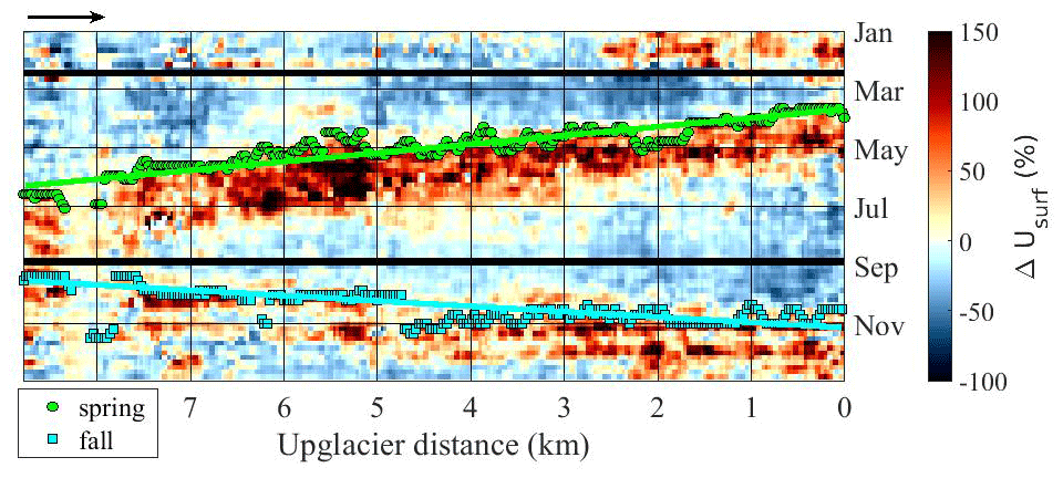
Figure 5 Illustration of our automatic picking of the onset of the spring/summer and autumn accelerations. The background is the annual pattern of relative changes in glacier velocity with respect to the annual median velocity along the flowline of the Malyy Tanymas Glacier (as in Fig. 4j). Round dots and squares show the automatically picked onset of the spring/summer and autumn accelerations, respectively. Green and light blue lines show the linear fits of the migration of accelerations as a function of along-flow distance. The black lines show the temporal limits to define the spring/summer and autumn periods.

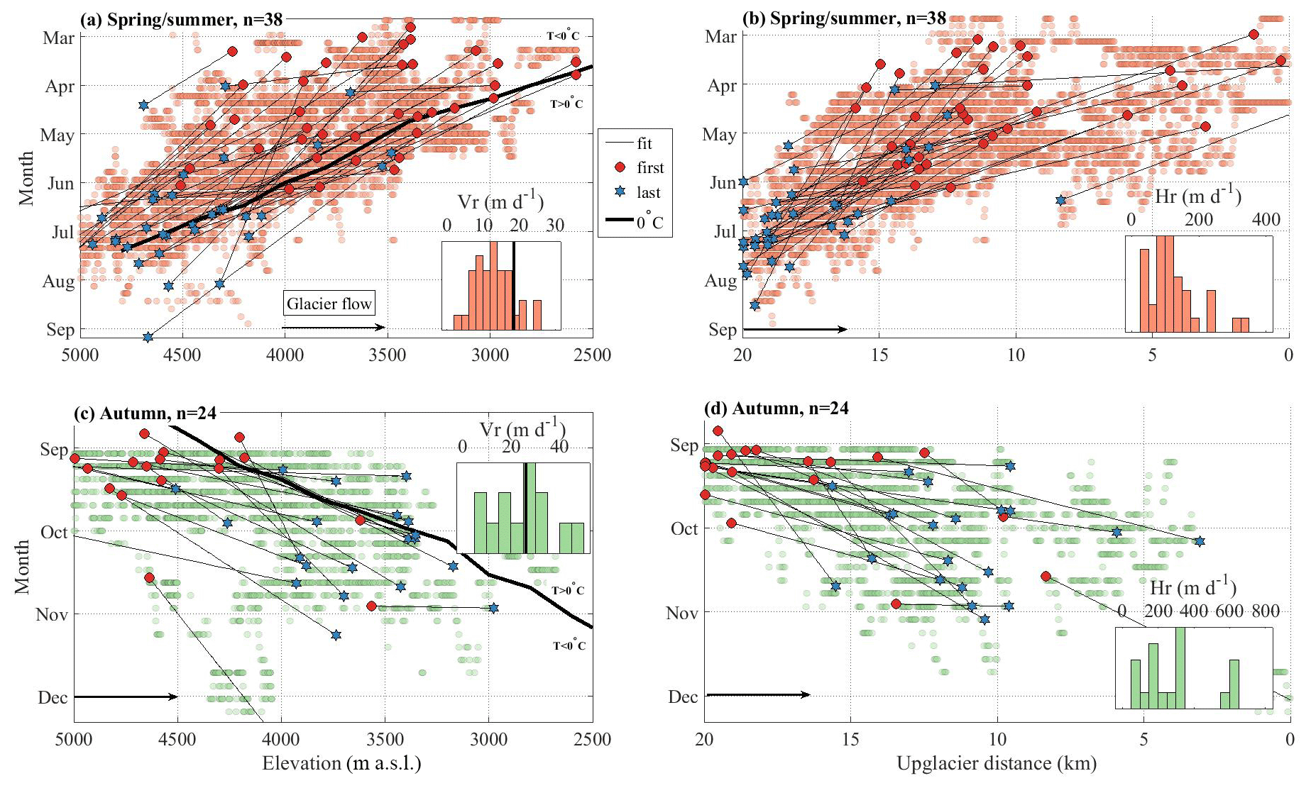
Figure 6 Observed time at which the acceleration starts along the flowline as a function of (a, c) the glacier elevation and (b, d) the upglacier distance for the spring/summer period (a, b) and the autumn period (c, d). Light orange and green dots show the automatically picked points (as described in Fig. 5), red points show the earliest onset date of the acceleration for each glacier and blue stars show the latest onset date obtained from the fitted line. Gray lines show the fitted migration rate of the acceleration along the flowline for each glacier. Histograms show the distribution of the vertical (Vr) and horizontal (Hr) migration rate. Bold black line in (a) shows the time and elevation at which daily averaged air temperature starts to be positive during the melt season; above this line temperatures are negative and under this line they are positive (Fig. S1). Bold black line in (c) shows the time and elevation at which air temperatures drop to negative values at the end of the melt season; above this line temperatures are positive and under this line they are negative (Fig. S1). Migration rates of these temperature changes with altitude are shown in bold black lines in the histograms.

4.3.2 Temporal characteristics

For the 38 glaciers that exhibit spring/summer accelerations, these usually starts between March and May at the glacier front and between June and August at higher altitudes, illustrating a clear upglacier migration (Fig. 6a, b). The rate at which the acceleration migrates with altitude (Fig. 6 a) is similar between glaciers (12±9 m d⁻¹) and comparable to the rate at which the mean daily air temperature increases with altitude in spring (18 m d⁻¹; black line in Fig. 6a). The onset of accelerations occurs about 1 month before the mean daily air temperature becomes positive (black line in Fig. 6a).

For the 24 glaciers that exhibit an autumn acceleration, it usually starts in September in the upper part of the glaciers and a few weeks to a few months later towards the glacier front, illustrating a downglacier migration (Fig. 6c, d). The rate at which this downglacier migration occurs (24±18 m d⁻¹) is twice as fast as the rate of upglacier migration during spring/summer. However, these rates are still comparable to the rate at which the mean daily air temperature decreases with altitude in autumn (24 m d⁻¹; black line in Fig. 6c; derived from the time series of temperature shown in Fig. S1). The onset of acceleration occurs within 1 month after the mean daily air temperature becomes negative (black line in Fig. 6c). Furthermore, we do not observe a significantly different geometry (i.e., slope, width, length, orientation, hypsometry) or glacier velocity between glaciers that exhibit such acceleration and those that do not (Fig. S5).

5 Discussion

5.1 Variations in migration rate

The onset time of the spring/summer accelerations appears to be positively correlated to the elevation at which it occurs (Fig. 6a, b): the accelerations start earlier at lower altitudes and they end later at higher altitudes (Fig. 7a, b). These trends do not appear to be influenced by the glacier orientation (marker color) or slope (marker size); instead, they appear to be similar to the trend in temperature change with altitude (solid lines in Fig. 7a, b). The acceleration generally starts in the 2 months before daily mean air temperatures reach positive values at the beginning of the melt season (Fig. 6a, b; Fig. 7a; R² of 0.17), and they reach their highest elevations when daily maximum air temperatures reach positive values at the end of the melt season (Fig. 6a, b; Fig. 7b; R² of 0.33). For some glaciers, the fraction (by length) of the glacier subject to acceleration appears to be positively related to the fraction of the glacier below the ELA (Fig. 7c). Glaciers that accelerate over 80 % to 100 % of their extent, however, defy this trend. The upglacier migration rate of the accelerations (i.e., the norm of the vertical and horizontal rates) appears to be negatively related to the slope of the glacier (Fig. 7d). In other words, the shallower the glacier slope, the faster the migration rate. When normalizing the migration rate by the glacier slope (Fig. 7d, c), we observe no obvious influence of the median glacier velocity on the migration rate (Fig. 7e) but a positive relation with the glacier width (Fig. 7f, R² of 0.63). However, when distinguishing by normalized migration rate, the migration rate tends to decrease with increasing glacier velocity for glaciers with a higher rate (> 1 km d⁻¹).

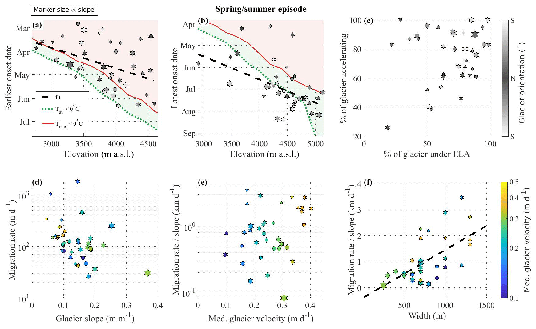
Figure 7 Characteristics of the upglacier migration rate of the spring/summer accelerations measured on 38 glaciers. (a) Earliest and (b) latest onset dates of the accelerations as a function of the glacier altitude where they occur. The dashed black lines show a linear fit with R² of 0.17 and 0.33 in (a) and (b), respectively. The red and green lines in (a) and (b) show when the daily maximum and daily mean temperature start to be positive during the melt season (Fig. S1). (c) Fraction of glacier length over which the acceleration is observed, relative to the fraction of glacier length below the ELA. Marker colors in (a)–(c) show glacier orientation. (d) Migration rate as a function of mean glacier slope. (e, f) Migration rate normalized by mean glacier slope as a function of median glacier velocity and glacier width, respectively. The dashed black line shows a linear fit with R² of 0.63. Marker colors in (d)–(f) show the median value of the velocity reached during the acceleration. The size of the marker represents the slope of the glacier: the smaller the marker, the shallower the slope.

Similar to the spring/summer accelerations, the timing of the autumn accelerations is related to the elevation at which it occurs (Fig. 6c, d): the acceleration starts earlier at higher altitudes and ends later at lower altitudes, thus depicting a clear downglacier migration. Most of the onset dates (∼80 %) occur after the daily mean air temperature has reached negative values at the end of the melt season (Fig. 8a, b). The fraction (by length) of the glacier subject to acceleration does not seem to depend significantly on the fraction of the glacier below the ELA (Fig. 8c). We observe that the autumn accelerations are restricted to a smaller and lower fraction of the glacier (Fig. 8c) than during the spring/summer accelerations, which is also indicated in Fig. 4. These patterns are not clearly influenced by the glacier slope (marker size) or the glacier orientation (marker color). As during the spring/summer accelerations, the migration rate of glacier acceleration appears to be negatively related to the glacier slope (Fig. 8d). When normalizing the migration rate with the slope of the glacier, the downglacier migration rate appears to be negatively correlated with the glacier velocity (Fig. 8e). As for the upglacier migration rates, we observe that downglacier migration rates increase with glacier width (Fig. 8f, R² of 0.68).

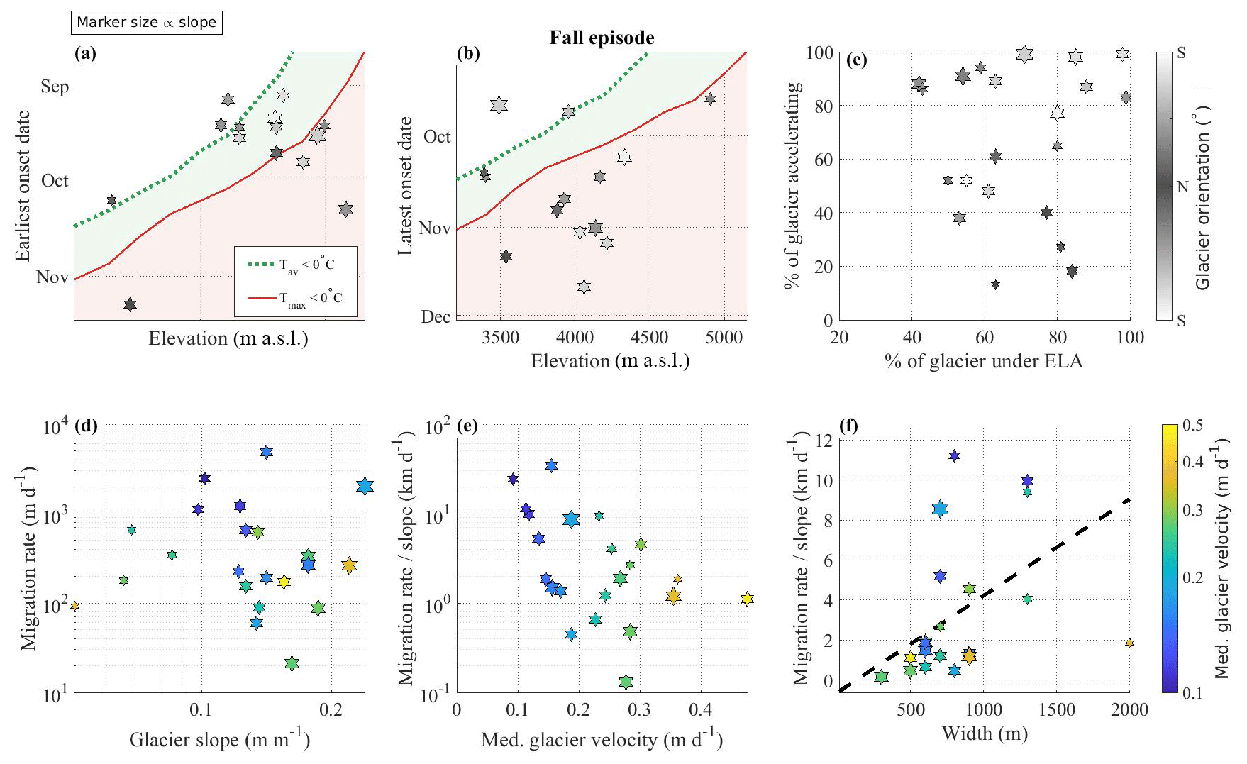
Figure 8 Characteristics of the downglacier migration rate of the autumn accelerations measured over 24 glaciers. (a) The earliest and (b) latest onset dates of acceleration as a function of glacier elevation where they occur. The red and green lines in (a), (b) show when the daily maximum and daily average start to be negative at the end of the melt season. (c) Fraction of glacier length over which acceleration is observed relative to the fraction of glacier length below the ELA. Marker colors in (a)–(c) show glacier orientation. (d) Migration rate as a function of mean glacier slope. (e, f) Migration rate normalized by mean glacier slope as a function of median glacier velocity and glacier width, respectively. The dashed black shows a linear fit with R² of 0.68. Marker colors in (d)–(f) show the median value of the velocity reached during the accelerations. The size of the marker represents the slope of the glacier: the smaller the marker, the shallower the glacier.

5.2 Causes of short-term velocity changes

5.2.1 Spring/summer

Of the 48 glaciers we studied, 38 of them show clear changes in glacier velocity between a slow winter period (November to February) and a fast spring/summer period (March to August), when many glaciers accelerate by up to 150 %–300 % (Figs. 3, 4). This behavior has already been observed on the Fedchenko Glacier (Lambrecht et al., 2014) and other large and/or fast-flowing mountain glaciers, for instance in the neighboring Karakoram Range (Quincey et al., 2009; Scherler and Strecker, 2012; Usman and Furuya, 2018), in the European Alps (Gordon et al., 1998; Vincent and Moreau, 2016), and in the Southern Alps of New Zealand (Purdie et al., 2008) or in Alaska (Armstrong et al., 2016), but it has not yet been documented on such a variety of mountain glaciers with high temporal resolution (Figs. 1, 4).

Our results show that the spring/summer accelerations are mainly confined to the ablation zone and depict an upglacier migration, which appears mainly controlled by altitude and air temperature (Figs. 4, 8). Elevation and air temperature are linearly related and exert a key control on melt rates, which is the main contributor to bed water supply in spring/summer (Yao et al., 2012; Lambrecht et al., 2018). Therefore, we suggest that the spring/summer accelerations are primarily caused by the evolution of the subglacial drainage system in response to changes in bed water supply. At the beginning of the melt season (March to May) and at low elevations (∼3000 m) the supply of meltwater to the bed increases rapidly due to positive air temperatures (Fig. S1) and inundates a likely inefficient drainage system, resulting in increased basal water pressure and consequently higher glacier velocity (Lliboutry, 1968; Iken and Bindschadler, 1986). This is supported by the earliest onset of acceleration at the lowest elevations (Figs. 6a, b, 7a). Later during the melt season, positive temperatures are also reached at higher altitude (Fig. 6) and the upper parts of the ablation zone are subject to an increased supply of meltwater to the bed, which likely induces an increase in basal slip. This is supported by the upglacier migration of the accelerations (Fig. 6) and the later onset of the acceleration at high elevations (Fig. 7a). Concomitantly, meltwater supply to the bed continues in the lower parts of the ablation zone, likely leading to the development of an efficient drainage system, which decreases the basal water pressure and thus the glacier velocity (Lliboutry, 1968; Iken and Bindschadler, 1986; Nanni et al., 2021). Indeed, a slowdown following an acceleration is observed towards the glacier front between May and July (Figs. 3, 4).

The spring/summer accelerations also appear to be influenced, although to a lesser extent, by glacier dynamics and geometry, as the rate of upglacier migration significantly increases with width and slightly decreases with glacier median velocity (Fig. 7d, e, f). Very fast migration rates (corrected by the influence of slope) mean that the accelerations occur almost at the same time along the entire length of the glacier. This kind of behavior could be promoted by glaciers where the drainage system responds quickly to water supply to the bed and/or the drainage system is very inefficient at the beginning of the melt season. Such conditions are expected for thick glaciers, which are typically also wide glaciers, as higher normal stresses promote the closure of the efficient drainage system during the winter period (Lliboutry, 1968), and for slow-moving glaciers where the drainage system is expected to be less efficient than for fast-moving glaciers (Kamb, 1987).

5.2.2 Autumn

Of the 48 glaciers we analyzed, 24 show clear acceleration in autumn, followed by a period of faster velocities (Figs. 3, 4, 5, 6). Such autumn accelerations have rarely been observed before, and we discuss potential causes here. As during spring/summer, the accelerations do not occur at the same time over the glacier. They often follow a downglacier migration related to the evolution of air temperature with elevation (Fig. 6c, d). The period of faster velocity subsequent to the autumn accelerations is of shorter duration (∼1 month) than the one following the spring/summer accelerations (∼ 1–4 months), and these faster velocities are often restricted to the lower part of the ablation zone (Figs. 6, 8).

Short acceleration periods during autumn (e.g., from days to weeks) have been observed previously and have been proposed to be caused by a reduced efficiency of the drainage system, making it more sensitive to sudden water supply (Hodge, 1974; Sugiyama and Gudmundsson, 2003; Harper et al., 2005; Hart et al., 2019). Gradual closure of the drainage system occurs when the water supply to the bed decreases and does not counteract the creep closure (Röthlisberger, 1972), which is probably the case of mountain glaciers at the end of the melt season (Nanni et al., 2020). As a consequence, the efficiency of the drainage system decreases, making it more sensitive to low water input. This process is consistent with the downglacier migration that we observe, as closure should first occur higher up, where meltwater inputs decrease earlier. It is also consistent with the fact that we observe such episodes mostly in the lower part of the glaciers, as enough water is needed for the drainage system to be pressurized again. This water input could be due to drainage from supraglacial ponds (Clason et al., 2015; Miles et al., 2018), rainfall events (Vieli et al., 2004; Horgan et al., 2015) or the gradual release of subglacially stored water, which has been observed to promote a sustained high velocity outside the melt season (Tedstone et al., 2013; Hart et al., 2019). In the western Pamirs, the autumn season is typically dry (Yao et al., 2012), making it unlikely that rainfall events are the main cause for the water input. Of the glaciers that exhibit this autumn acceleration, around 50 % have an ablation zone with significant debris cover (Mölg et al., 2018) and most of them show the presence of supraglacial ponds in the upper ablation zone (Fig. S7). Such ponds are generally small (< 100 m wide) and are similar to those observed in the Himalayan regions where the ice is crevassed and/or debris covered (Iwata et al., 1980; Sakai et al., 2000; Miles et al., 2017). Supraglacial ponds tend to form during the summer period and drain in late summer and/or early autumn (Miles et al., 2018), which is consistent with the timing of the autumn acceleration. We hypothesize that these drainage events could contribute to the sudden influx of meltwater to the bed in autumn. Water storage in firn has also been observed to delay runoff from days to months (Jansson et al., 2003); however very few studies have been conducted in the Pamir region, which makes it difficult for us to assess the extent to which water storage may occur in firn.

We therefore suggest that the autumnal accelerations result from glacier instability occurring in the upper ablation zone and propagating down the glacier. This instability could be caused by a sudden influx of meltwater, as discussed above, which triggers a local increase in basal water pressure, facilitated by a reduced capacity of the drainage system. Such a sudden change can be clearly seen in Fig. 5, with a rapid increase in velocity directly followed by a drop. This leads locally to a rapid change in basal stress, which can promote the propagation of an instability in a manner similar to surges (Thøgersen et al., 2019; Beaud et al., 2022) or glacier response to calving (Riel et al., 2021). The downward propagation reaches migration rates similar to those observed on alpine glaciers in the form of a kinematic wave (Hewitt and Fowler, 2008), which supports our hypothesis of a local disturbance. Such sensitivity to local disturbances may be favored by soft-bedded glaciers, which is probably the case of the glaciers studied because 70 % of them are suggested to be surge type glaciers because of soft beds (Goerlich et al., 2020). If our hypothesis that meltwater input by supraglacial pond drainage holds true, these events could represent the lower end of hydraulically controlled surges and glacial lake outburst floods (GLOFs), which play an important role in mountain natural hazards (Iribarren et al., 2018; Kääb et al., 2018; Bhambri et al., 2019; Yang et al., 2022).

5.3 Limits and opportunities in monitoring short-term velocity changes

Our approach resolves peak velocity changes as low as ±0.1 m d⁻¹ (36.5 m yr⁻¹) for glaciers with a median velocity as low 0.1 m d⁻¹ (Figs. 1, 4). Where the median velocity is of the order of 0.2 m d⁻¹ (73 m yr⁻¹), the observed accelerations can be as low as 25 % (0.05 m d⁻¹, 18.25 m yr⁻¹). We observe such changes for large glaciers (e.g., Fedchenko Glacier) but more importantly also for small glaciers that are less than 5 km long and 250 m wide (Fig. 4e). With pixel sizes of 10 and 15 m, for Sentinel-2 and Landsat 8, respectively, this corresponds to a precision of $\mathrm{1}/\mathrm{10}$th to $\mathrm{1}/\mathrm{15}$th of the pixel for low-velocity areas (∼0.1 m d⁻¹) and of $\mathrm{1}/\mathrm{20}$th to $\mathrm{1}/\mathrm{30}$th of the pixel for mid-to-fast-velocity areas (> 0.2 m d⁻¹). Such a sub-pixel image matching precision is higher than the 0.15 to 0.33 pixels that we calculated based on stable ground analysis (Fig. 2). It is also higher than the 0.1 pixel precision previously estimated for mountain areas (Scherler et al., 2008; Heid and Kääb, 2012). We suggest that the high precision we obtain when investigating peak velocity has two reasons. On the one hand, the stable-ground estimation might overestimate the error, especially in our mountainous study area where the standard deviation over ice-free areas can also be affected by natural surface displacement such as hillslope movements or riverbed changes. The precision obtained over glaciated area, where most of the displacements are caused by glacier flow, should not be influenced by displacements observed over ice-free areas and could therefore be higher (more precise). In addition, glaciers typically have lower slopes than their surroundings, which reduces the impact of inaccuracies in the elevation model used for the orthorectification (Scherler et al., 2008). Indeed, we observe significant changes in surface velocity of less than 0.1 m d⁻¹ over the shallow-sloping ablation zone over 10 to 20 d periods (Fig. 4). This higher precision could also be due to faster-flowing glaciers and more textured surfaces in the ablation zone compared to the accumulation zone and stable ground (Figs. S8, S9). On the other hand, we suggest that by combining multiple measurements (different sensors, time periods and years), we obtain an improved signal of seasonal and recurring glacier velocity changes. Such an approach has been shown to significantly increase measurement precision (Altena et al., 2019; Derkacheva et al., 2020). We have observed that Sentinel-2 imagery can help to resolve patterns that are only hinted at using Landsat 8 alone. However, the increase in spatial and temporal resolution obtained with the Sentinel-2 imagery does not offer a significant advantage, as shown by the similar resolution we obtain (Fig. 2). We suggest that further improvement in our protocol could be made using the approaches presented in Altena et al. (2019) and Derkacheva et al. (2020), which would allow combining velocity obtained from different sensors and over different time spans with more advanced statistical approaches. The incorporation of radar images in combination with optical images (Derkacheva et al., 2020) would also increase the accuracy of the velocity field as radar images can be used even for time periods with cloud cover.

The high precision we obtain shows the advantage of combining a statistical approach with a robust measurement of surface displacement to improve the level of comprehension of large satellite imagery datasets. This is made possible by the COSI-Corr algorithm and the medium-resolution high-quality satellite imagery we have used. This approach takes advantage of the large remote-sensing datasets that are now available and thus allows monitoring short-term (down to 10 d) changes in mountain glacier velocity, even for relatively slow-flowing glaciers (0.1 m d⁻¹) and/or on the slower parts of glaciers.

6 Conclusions

Our study demonstrates that the large amount of optical imagery that is now available from satellite programs such as Landsat 8 and Sentinel-2 can be effectively exploited to monitor surface velocity of mountain glaciers with a resolution down to 10 d. Our protocol requires minimal manual processing and is effective for a wide range of glacier geometries, from small (∼250 m wide, 5 km long) to large (> 50 km long). This protocol is not only applicable to glaciers but also to other types of surface movements. We observed a clear pattern of seasonal velocity changes that repeats over 7 years on 38 glaciers in the western Pamirs, with accelerations in spring–summer that start at the glacier front and propagate upwards. The upglacier migration rate correlates with the air warming rate, which supports a climatic driver. We link these accelerations to changes in the subglacial drainage system in response to changes in meltwater supply to the bed. We also observed autumn acceleration episodes on 24 glaciers that occur on an annual basis in the ablation zone and where the accelerations propagate downglacier, concurrent with the air-cooling rate. We link these acceleration episodes to local glacier instabilities, probably caused by drainage of supraglacial ponds and changes in drainage system efficiency. This shows the potential of our approach to investigate not only the well-known seasonal acceleration but also shorter-term dynamics, which it is crucial to capture in order to study the response of glaciers to changes in air temperature.