Central Asia's spatiotemporal glacier response ambiguity due to data inconsistencies and regional simplifications

We have investigated the drivers behind the observed spatiotemporal mass balance heterogeneity in Tien Shan and Pamir, in High Mountain Asia. To study the consistency of the different interpretations derived from the available meteorological reanalysis and remote sensing products, we used correlation analyses between climatic and static drivers with novel estimates of region-wide annual glacier mass balance time series. These analyses were performed both spatially using different spatial classifications of glaciers and temporally for each individual glacier. Our results show that the importance of the variables studied depends strongly on the dataset used and which spatial classification of glaciers is chosen. This extends to opposing results using the different products. Even supposedly similar datasets lead to different and partly contradicting assumptions on dominant drivers of mass balance variability. The apparent but false consistencies across studies using a single dataset are related, according to our results, to the chosen dataset or spatial classification rather than to the processes or involved environmental variables. Without a glaciological, meteorological, and hydrological in situ observation network providing data that allow for the direct calibration and validation of extensive datasets, our understanding of neither the changing cryosphere at the regional scale for Tien Shan and Pamir nor glacier response to climate change or the assessment of water availability for the region’s growing population can improve.

1 Introduction

Glaciers across Tien Shan and Pamir, in High Mountain Asia, have been observed to change heterogeneously in space (e.g., Barandun et al., 2021a; Shean et al., 2020; Brun et al., 2017; Miles et al., 2021). Under the assumption of equal climatology, glacier morphology has been found to explain up to 36 % of the mass balance variability for Tien Shan, 20 % for Pamir-Alay, and only 8 % for Western and Eastern Pamir (Brun et al., 2019). Thus, local topographic and glacier-specific morphological characteristics cannot wholly explain the diverse glacier responses to climate change (Fujita and Nuimura, 2011; Brun et al., 2019); these are also related to sharp contrasts in the local climatological settings, mainly to their different mass balance sensitivities to climate (Sakai and Fujita, 2017; Wang et al., 2019) (responsible for up to 60 % of spatially contrasting glacier response in High Mountain Asia; Sakai and Fujita, 2017). Mölg et al. (2014) and Farinotti et al. (2020) related a spatially heterogeneous glacier response for selected mountain ranges to different weather pattern constellations. These are reported to have changed in the past (Gerlitz et al., 2020), leading to increased climate variability; de Kok et al. (2020) argue that increased evapotranspiration might explain positive mass balances for solid-precipitation-sensitive glaciers. However, systematic analyses of drivers behind the observed spatiotemporal mass balance heterogeneity have attracted limited attention to date mainly due to (1) limited direct glaciological and meteorological measurements, (2) large uncertainties about meteorological variables, and (3) limited understanding of nonclimatic effects on glacier mass balance.

1. Glaciological measurements are conducted predominantly at an annual resolution and are limited to a few well-accessible glaciers. Geodetic methods, which have become state of the art to assess glacier mass balances, have a limited temporal resolution. Remote sensing provides a powerful tool to study inaccessible glaciers from space; however, robust mass change assessments remain limited to intervals of 5 years or more (e.g., Kääb et al., 2015; Brun et al., 2017; Wang et al., 2017; Shean et al., 2020; Wouters et al., 2019; Hugonnet et al., 2021). Barandun et al. (2021a) highlighted hotspots of spatiotemporal heterogeneity and increased mass balance variability in the different mountain ranges of Tien Shan and Pamir at an annual temporal resolution; however, their results were not purely observation based. Meteorological measurements are sparse and often discontinuous even for the most monitored glaciers in Central Asia, such as Abramov or Golubin glaciers (Kronenberg et al., 2021; Azisov et al., 2022). Replacement of old meteorological stations with modern sensors often lacks precise homogenization. Regional extrapolation from station data and use of existing time series as validation datasets for gridded products are thus problematic.

2. Identification of potential climatic drivers for mass balance variability is highly complicated; uncertainties in climatic state variables prevail due to the abovementioned lack of independent station data in the remote and largely inaccessible terrain. These data are crucial for validation and adjustment of gridded datasets (Zandler et al., 2019). Precipitation products, in particular from reanalysis, interpolation, and remote sensing, can show up to 1000 % difference in these remote locations (Palazzi et al., 2013; Pohl et al., 2015; Immerzeel et al., 2015) and can barely cover the large range of orographic processes that affect, for example, small-scale precipitation events (Roe et al., 2003). Reanalysis products, in most cases, are more suitable for capturing precipitation seasonality and spatial patterns in Pamir – albeit with overall intensities possibly not being well captured – due to problems in remote sensing snow retrieval, as well as precipitation in general, over complex topography (Zandler et al., 2019; Pohl et al., 2015). The spatiotemporal comprehensiveness of reanalysis data facilitates the inclusion of various climatic variables at a global scale in correlation analysis that is otherwise not available from simple meteorological stations or remote sensing/interpolation data products (e.g., Hugonnet et al., 2021).

3. Many glaciers in Central Asia are heavily debris covered with considerably different debris thicknesses (Kraaijenbrink et al., 2017; McCarthy et al., 2021). A scale-dependent debris cover–mass balance relationship and limited region-wide debris thickness assessments restrict the explanatory power of debris cover for region-wide glacier mass balance patterns in Central Asia (Brun et al., 2019; Miles et al., 2022). Both Tien Shan and Pamir are known to host numerous surge-type glaciers (Mukherjee et al., 2017; Kotlyakov et al., 2008; Gardelle et al., 2012; Guillet et al., 2022). After a surge, the mass balance regime of a glacier changes abruptly due to nonclimatic reasons. After such a pronounced advance, melt rates might increase greatly, uncoupled from current local climate conditions (Glasser et al., 2022). Guillet et al. (2022) show that no significant difference exists in mass balance between surge- and nonsurge-type glaciers. Avalanching represents another nonclimatic factor that influences glacier mass balance through mass redistribution. The quantification of its effect on glacier mass balance at regional scales is, however, not straightforward. As an approximation, Brun et al. (2019) used the avalanche contributing area as a potential morphological control. However, the authors found no significant correlation with their mass balance estimates for almost all regions assessed in High Mountain Asia.

The reasons mentioned above outline a lack of consistent understanding regarding the climatic and nonclimatic drivers of glacier mass balance variability in Tien Shan and Pamir. Therefore, a more comprehensive and rigorous analysis of the available datasets is indispensable to provide more conclusive and accurate results and interpretations on the drivers of glacier response to climate change in Central Asia. Therefore, we aim in this study for a rigorous analysis of different datasets to identify similarities and differences in the drivers found to explain the glacier mass balance changes in Pamir and Tien Shan, with the ultimate goal of advancing the understanding of the drivers behind heterogeneous mass balance changes in Central Asia. Our analysis benefits from newly available and advanced highly temporally resolved mass balance estimates and new reanalysis products. Given the often unconstrained uncertainties in climatological/meteorological datasets for data-sparse regions, we analyze (1) the consistency of the different meteorological and mass balance datasets and (2) which variables can explain in a statistically significant manner the variability found in mass balance datasets.

We follow a systematical approach to test three different reanalysis products that are or have been used extensively in the region. Additionally, due to existing differences in glacier mass balance time series, we incorporate the two available annual mass balance estimates for the region: the snowline-aided estimates by Barandun et al. (2021a) and the geodetic mass balances by Hugonnet et al. (2021). Mass balance time series are related to the most commonly used climatic variables of temperature (T) and precipitation (P) from the reanalysis datasets, snow cover (SC) from a remote sensing product, and glacier-specific topographic and morphological characteristics. Finally, to account for possible regional data issues or arbitrarily chosen regional divisions, the analyses are performed at different spatial subsets.

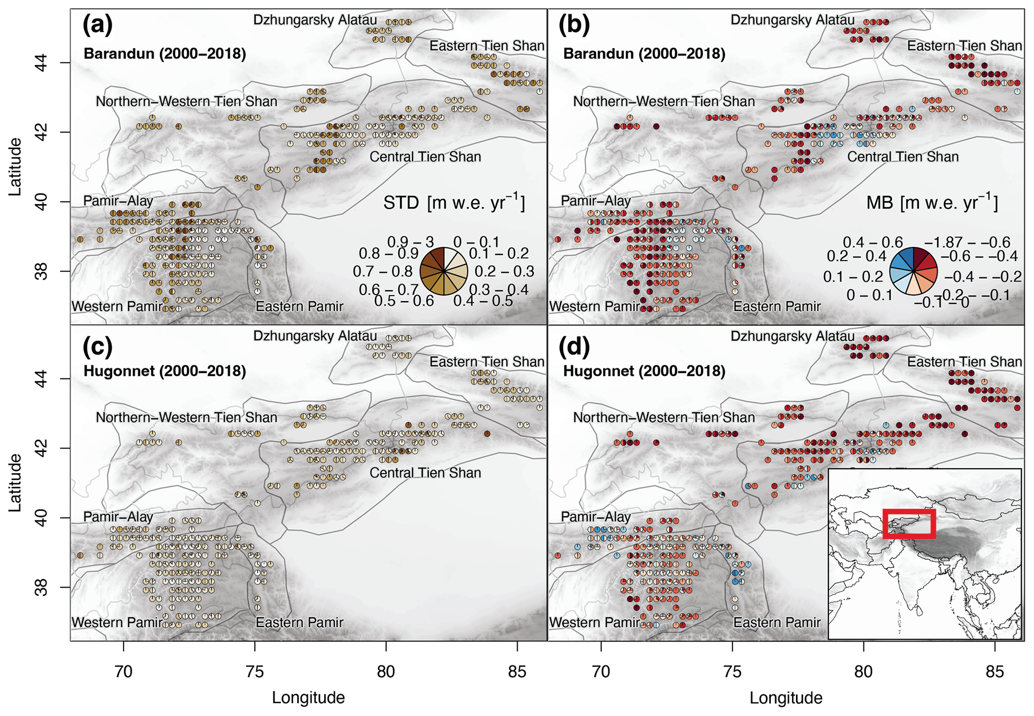
Figure 1 Overview map of the study region. (a, c) Glacier mass balance variability in terms of standard deviation (SD) and (b, d) average glacier mass balance (MB) estimates (a, b) from Barandun et al. (2021a) and (c, d) Hugonnet et al. (2021). Estimates from Hugonnet et al. (2021) include only the glaciers for which the transient-snowline-constrained modeling of Barandun et al. (2021a) provides estimates. The pie charts aggregate values per glacier into classes and the relative class frequencies. Pie charts are not scaled to glacier area. The seven subregions of the Hindu Kush Himalayan Monitoring and Assessment Programme (HIMAP) classification (Bolch et al., 2019) are shown in grey outlines.

2 Study sites and data

2.1 Study sites

2.1.1 Climate setting and variability

Central Asia is a mostly arid–semiarid region (Barry, 1992) with high seasonal precipitation variability due to its continentality (Haag et al., 2019). Synoptic large-scale meteorological conditions in Central Asia respond to the main direction of the zonal flow of the air masses from west to east. A deflection of westerly trade winds (westerlies) to the north and south at the western orogen margin of Tien Shan and Pamir causes intense precipitation in the west, and a barrier effect creates increasingly arid conditions towards the central and eastern part of the main mountain ranges (Pohl et al., 2015; Aizen et al., 2009, 1995). Meridional airflow can occur when tropical air masses enter from the south and southwest or when northwesterly, northerly, and sometimes even northeasterly cold air masses intrude into Central Asia (Schiemann et al., 2008, 2007). These mechanisms can provide some insights into the complex climate settings of High Mountain Asia that reanalysis products are expected to depict. These settings range from humid and maritime to continental and hyperarid (Bohner, 2006; Schiemann et al., 2007; Yao et al., 2012; Maussion et al., 2014).

Climate variability depends strongly on how and when the different weather types interact (Zhao et al., 2014; Wei et al., 2017; Gerlitz et al., 2020), guided principally by the position and strength of the jet stream. Schiemann et al. (2008) investigated in detail the seasonal cycle of Central Asian climate to show that the jet stream is situated over the north of Central Asia during the summer months and moves towards the south in autumn, creating atmospheric instabilities. Resulting precipitation occurs mainly at the western margin until mid-January. Subsequently, the influence of the jet stream weakens over Central Asia, and the Siberian high-pressure system creates clear and calm winter weather, especially reducing winter precipitation in the north and east (Aizen et al., 1997). By the end of February, the jet stream returns northwards and reaches the southern edge of Central Asia carrying warm and moist air. This creates temperature contrasts between the north and the south and strengthens the cyclonic activity over Central Asia (Schiemann et al., 2008). Consequently, the highest amount of precipitation, characterized by heavy showers and thunderstorms, occurs in March and April, culminating at the western parts of Tien Shan and Pamir. While the jet stream continues northwards during May, precipitation maxima are reached in Northern Tien Shan in June (Aizen et al., 2001). At the beginning of the summer, the cyclonic activity weakens, and heat lows start to form again. During summer, the Siberian anticyclonic circulation provides cold and moist air masses in Northern, Central, and Eastern Tien Shan, resulting in frequent spring or summer precipitation (Aizen et al., 1997). The most dominant moisture source at the southern margins of Pamir is the heavy rainfalls provided by the Indian summer monsoon (e.g., Cadet, 1979). Orographic shielding at the south and southeastern margin of Central Asia's mountain ranges strongly reduces this moisture supply and leads to very dry conditions in the central parts of Pamir (Boos and Kuang, 2010; Haag et al., 2019). The Tibetan anticyclone additionally influences the local climate along the eastern margin of Pamir (Archer and Fowler, 2004), leading to summer cooling (Forsythe et al., 2017) and summer rainfall (Aizen et al., 1997).

2.1.2 Topography and glaciation

Tien Shan and Pamir are the two main mountain ranges of Central Asia north of the Karakoram and Hindu Kush. In the present work, we choose a subdivision of the regions based on the commonly used Hindu Kush Himalayan Monitoring and Assessment Programme (HIMAP) regional division suggested in Bolch et al. (2019): Northern–Western Tien Shan, Eastern Tien Shan, Central Tien Shan, Dzhungarsky Alatau, Pamir-Alay, Western Pamir, and Eastern Pamir (Fig. 1). Tien Shan hosts almost 15 000 glaciers, covering a surface area of ≈12 300 km² (RGI, 2017a). Pamir, including Pamir-Alay (also Hissar-Alay), hosts around 13 000 glaciers, covering similarly a surface area of ≈12 000 km². The highest mountain ranges are found in Central Tien Shan and Western and Eastern Pamir, and the mass turnover is decreasing along a gradient of increasing continentality. Tien Shan and Pamir are typically classified as subcontinental–continental (western and northern part of Tien Shan and Pamir-Alay; central part of Tien Shan and central and eastern part of Pamir) glacier regimes (Wang et al., 2019). Barandun et al. (2021a) showed similar mass losses for Tien Shan and Pamir. Mass balance estimates of Barandun et al. (2021a) show the least negative mass balances from 2000 to 2018 to be in Central Tien Shan ($-\mathrm{0.13}\pm \mathrm{0.37}$ m w.e. yr⁻¹) and Eastern Pamir ($-\mathrm{0.12}\pm \mathrm{0.37}$ m w.e. yr⁻¹). Dzhungarsky Alatau ($-\mathrm{0.46}\pm \mathrm{0.37}$ m w.e. yr⁻¹) and Eastern Tien Shan ($-\mathrm{0.48}\pm \mathrm{0.37}$ m w.e. yr⁻¹) are the subregions with the strongest mass loss; mass balances for Pamir-Alay ($-\mathrm{0.32}\pm \mathrm{0.37}$ m w.e. yr⁻¹), Western Pamir ($-\mathrm{0.25}\pm \mathrm{0.37}$ m w.e. yr⁻¹), and Northern–Western Tien Shan ($-\mathrm{0.30}\pm \mathrm{0.37}$ m w.e. yr⁻¹) are close to the region-wide average of the time period (from 2000 to 2018).

2.2 Data

2.2.1 Annual mass balance time series

In the present study, we use the two existing annually resolved glacier-specific datasets for glacier mass balance estimates covering all of Tien Shan and Pamir: one based on transient-snowline observations and geodetic mass balances and the other based on digital elevation model (DEM) differences (Fig. 1).

The first dataset (MB_Barandunetal) comprises the annual time series provided by Barandun et al. (2021a), who used a mass balance model calibrated simultaneously with transient snowlines (as a proxy for surface mass balance) and geodetic mass changes. The model was driven with ERA-Interim reanalysis data (Dee et al., 2011) for each glacier and year separately (Barandun et al., 2021a, 2018). ERA-Interim was chosen because, unlike other reanalysis products (e.g., ERA5), in situ observations in mountain regions are assimilated (Orsolini et al., 2019). Barandun et al. (2021a) provided annual mass balance time series, closely tied to direct observations, with low sensitivity to meteorological input for roughly 60 % of the glaciers larger than 2 km² in the data-sparse Tien Shan and Pamir regions. For more details the reader is referred to Barandun et al. (2018, 2021a) for the methodological approaches for mass balance determination and model sensitivity, to Naegeli et al. (2019) for the automatic snowline mapping, and to Girod et al. (2017) and McNabb et al. (2019) for the geodetic estimates. Differences in ERA-Interim and ERA5 performance and output at high altitudes are highlighted in Orsolini et al. (2019) and Liu et al. (2021), showcasing the independence of the two datasets.

The second dataset (MB_Hugonnetetal) comprises the geodetic mass balance estimates by Hugonnet et al. (2021), which rely on DEM differences and filtering techniques. The predominant input is the 20-year-long archive of stereo images from the Advanced Spaceborne Thermal Emission and Reflection Radiometer (ASTER) used to derive time series of DEMs. Their estimates were validated at all glaciers worldwide with intersecting laser altimetry and elevations derived from high-resolution optical imagery data. The approach shows good agreement at the global scale, although it has varying uncertainties at the regional scale (Hugonnet et al., 2021) due to a sometimes limited performance of the method for individual glaciers (Hugonnet et al., 2021). Geodetic methods are more accurate at longer timescales as the signal-to-noise ratio improves. However, Hugonnet et al. (2021) also provide annual estimates connected to much higher uncertainties pointed out by the authors, which we use in this work. We select only the glaciers from this dataset for which estimates from Barandun et al. (2021a) are available. This serves as a consistent analysis of dominant drivers and to highlight the differences between the two mass balance estimates (Fig. 2).

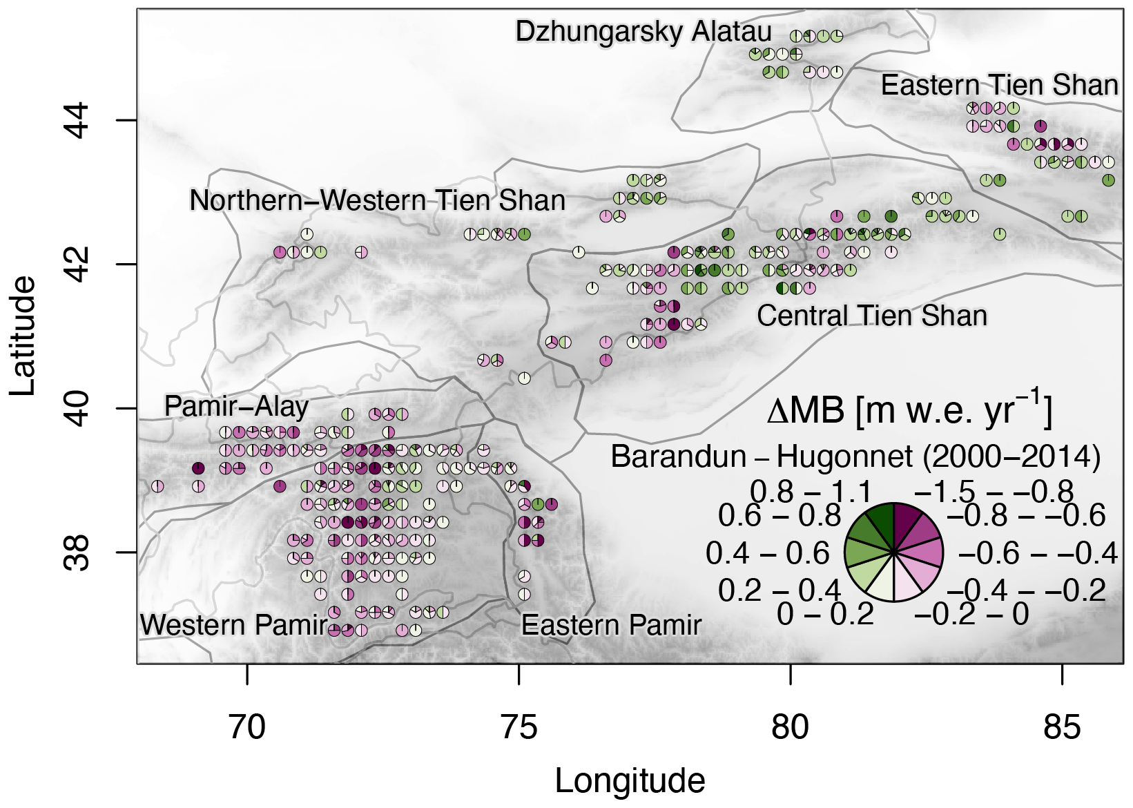
Figure 2 Difference in mean annual glacier mass balance between Barandun et al. (2021a) and Hugonnet et al. (2021) for the period 2000–2014 (see Fig. A1 for the period 2000–2018). Estimates from Hugonnet et al. (2021) only include the glaciers for which the transient-snowline-constrained modeling of Barandun et al. (2021a) provides estimates. The pie charts aggregate values per glacier into classes and the relative class frequencies. Pie charts are not scaled to glacier area.

Both datasets are tied to elevated uncertainties of the annual mass balance estimates. Barandun et al. (2021a) adopted mean uncertainties provided in Barandun et al. (2018) (±0.32 m w.e. yr⁻¹) associated with the snowline-constrained mass balance modeling and combined them with the error estimate from the geodetic surveys. This resulted in a rather conservative uncertainty of ±0.37 m w.e. yr⁻¹ and does not assume independence of the errors from year to year. Hugonnet et al. (2021) reported uncertainties of up to ±0.1 m w.e. yr⁻¹ for mean annual mass balance values of 5-year periods. Hugonnet et al. (2021) provide uncertainties in mass changes for periods shorter than 5 years only for the global or near-global estimates. Global annual mass balance uncertainties are reported to be around ±0.2 m w.e. yr⁻¹ (Hugonnet et al., 2021), and we expect higher ones for the mass balance time series of individual glaciers.

2.2.2 Glacier morphological characteristics

We use glacier outlines and areas from version 6 of the Randolph Glacier Inventory (RGI) (RGIv6; RGI, 2017a), kept unchanged over time, and the freely available void-filled Shuttle Radar Topography Mission (SRTM; Jarvis et al., 2008) digital elevation model as topographic input. We use the information provided in Scherler et al. (2018a) on the percentage of debris cover on individual glaciers for Tien Shan and Pamir and the data on surge activity from Guillet et al. (2022). The latter work provides multiple statistics on surge activity. We use occurrence of surge activity provided in this dataset to test whether a significant difference exists between surge- and nonsurge-type glacier mass balances in MB_Hugonnetetal and MB_Barandunetal. We do not include other variables such as avalanche processes due to insufficient data availability.

2.2.3 Meteorological data

We use precipitation and air temperature of three different reanalysis datasets to identify similarities and differences in the relationships of mass balance with key meteorological drivers (Figs. 3 and A2). The reanalysis products are (1) the European Centre for Medium-Range Weather Forecast (ECMWF) fifth-generation atmospheric reanalysis (ERA5) (Hersbach et al., 2020), (2) version 2.1 of the Climatologies at high resolution for the earth's land surface areas (CHELSA) time series (Karger et al., 2017, 2021), and (3) version 1.4 of the High Asia Refined (HAR) analysis at a 30 km spatial resolution (HAR30) (Maussion et al., 2011). The study time period is 2000–2018 (“long”) and 2000–2014 (“short”) for all datasets to match the limited temporal availability of HAR30 v1.4 (Maussion et al., 2011), for which only the second period was analyzed.

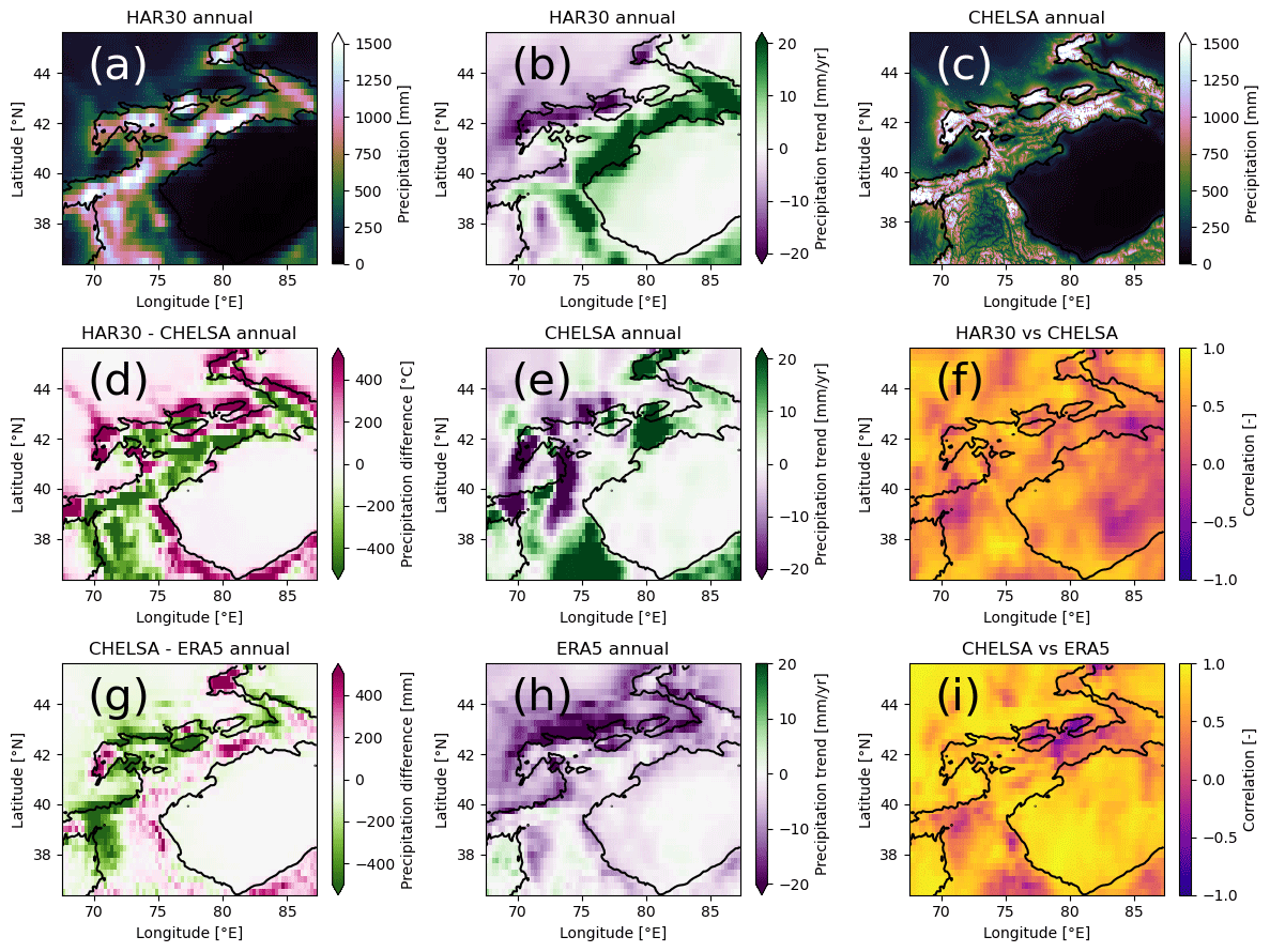
Figure 3 Sums of mean annual precipitation for (a) HAR30 and (c) CHELSA. Trends for (b) HAR30, (e) CHELSA, and (h) ERA5. Differences between (d) HAR30 and CHELSA and (g) CHELSA and ERA5 and the correlation between (f) HAR30 and CHELSA and (i) CHELSA and ERA5. CHELSA and ERA5 were spatially resampled bilinearly to the resolution of HAR30 for the differences and correlation. Black outlines correspond to 2000 m a.s.l. altitude. The same figure for temperature is provided in the Appendix (Fig. A2).

ERA5 monthly averaged data on single levels from 1979 to the present create an atmosphere reanalysis dataset (Hersbach et al., 2020) with a 0.25^∘ × 0.25^∘ (≈21 km) native spatial resolution. ERA5 incorporates a multitude of in situ and remote sensing data in an integrated forecasting system to produce hourly outputs of atmospheric variables. We obtained the monthly mean (sum) product from the ECMWF data store for temperature (precipitation). ERA5 data have not been thoroughly validated in hydrological or glaciological model applications in Pamir or Tien Shan. A significant overestimation of snow depth (Wang et al., 2021; Orsolini et al., 2019) is problematic for these applications and is also assumed to alternate the energy fluxes related to overestimated albedo (Wang et al., 2021). This renders the parameters for in- and outgoing energy fluxes problematic, and they are not consistently measured at the few meteorological stations in High Mountain Asia; we focus only on the two variables P and 2 m T. For our correlation analysis, a systematic and linearly scaled over-/underestimation does not pose a problem. Consequently, we focus on P and T for the other datasets too.

CHELSA time series version 2.1 is a processed and downscaled version of the ERA5 dataset which incorporates directional wind speeds and cloud cover observations to address precipitation biases and wind and leeward distributions (Karger et al., 2017). The final downscaled product presents a ≈1 km spatial and a monthly temporal resolution. By incorporating the CHELSA data, we provide a means to determine how state-of-the-art downscaling affects the correlation analysis.

HAR30 version 1.4 (Maussion et al., 2011) presents a 30 km spatial and a daily temporal resolution. Data result from a dynamical downscaling of global analysis data (final analysis data from the Global Forecasting System; National Centers for Environmental Prediction, National Weather Service, NOAA, 2000; dataset ds083.2) using the Weather Research and Forecasting–Advanced Research WRF (WRF–ARW) model (Skamarock and Klemp, 2008). The dataset has shown high consistency with temperature, precipitation, and snow cover measurements in several regions of High Mountain Asia, where uncertainties are especially large due to limited or nonexistent meteorological stations. This dataset has captured climatic extremes in the greater Pamir region that lead to floods and droughts (Pohl et al., 2015), has been used for glacier studies in the greater Himalayan region (Maussion et al., 2011; Mölg et al., 2014; Curio et al., 2015), and has been applied in hydrological studies (Pohl et al., 2015, 2017; Biskop et al., 2016). Despite the need to bias-correct HAR precipitation intensities in Pamir (Pohl et al., 2015) and the Tibetan Plateau (Biskop et al., 2016), the dataset has shown better correlation with in situ measurements than interpolated and remote sensing datasets in Pamir (Pohl et al., 2015). Due to large uncertainties in gridded meteorological datasets, we believe that the HAR dataset, validated at least to some degree in High Mountain Asia in several previous studies (e.g., Pohl et al., 2015, 2017; Biskop et al., 2016; Maussion et al., 2014), should be included in our analysis. We do not use HAR version 2 because ERA5 is used as input to downscale the version 2 output and shows strong differences with the validated HAR version 1 dataset.

2.2.4 Snow cover data

The snow cover product used in the present work is the Moderate Resolution Imaging Spectroradiometer (MODIS) monthly snow cover product MOD10CM version 6 (Hall and Riggs, 2015). MOD10CM is a monthly average snow cover dataset on a regular climate modeling grid with an approximately 5 km spatial resolution (Hall and Riggs, 2015). The snow cover is calculated using the Normalized Difference Snow Index (NDSI) constrained to positive values, providing snow cover values in the range between 0 % and 100 %. From the original snow cover fraction values, we also derive the temporal changes between consecutive time steps as a measure for snow accumulation or depletion events. Here, we refer to both variables as SC.

3 Methods

The mass balance estimates of Hugonnet et al. (2021) and Barandun et al. (2021a) provide average long-term values for the two study periods (2000–2014 and 2000–2018) and, more importantly, annual time series for individual glaciers that are only available from the year 2000 onwards. In turn, this allows us to run two kinds of analyses to determine potential drivers of mass balance variability: (1) a temporal individual analysis for each glacier correlating mass balance and meteorological time series and (2) a spatial analysis relating mean glacier mass balance with statistics of meteorological and morphological data, e.g., long-term averages, trends, or the standard deviation as a measure for mass balance or meteorological variability. Both types of analyses are based on multiple linear regression analysis to identify significant predictors in the group of meteorological or morphological variables (Fig. 4). In this study, we focus strictly on the determination of significant predictors in multiple linear regression analysis and neither report nor discuss obtained model coefficients or coefficients of determination in detail. This decision responds to the large uncertainties present in the outcomes of the analyses, as shown in the results. Focusing on whether variables show or do not show significant correlations allows for a streamlined highlighting of important variables and seasons.

For the correlation, each glacier provides a data point in the spatial analysis, and each time step of an individual glacier time series provides a data point in the temporal analysis. To systematically identify all significant (always at a significance level of α=0.05) independent variables while accounting for some complexity in glacier accumulation and ablation processes, we use all possible combinations of two independent predictors for each meteorological and morphological dataset. For the spatial analyses we report the number of identified significant predictor variables over the total number of variable combinations and refer to this as “relative importance”; for the temporal analyses, we identify all occurrences of significant predictor variables and present their frequency in pie chart maps. For the meteorological analysis, we constrain the variable combinations separately to each individual dataset product, i.e., only combinations from ERA5 or HAR or CHELSA. However, we also extend this analysis by adding the MODIS SC data to each reanalysis dataset in a second step. This allows for exploring whether the observational SC dataset adds more explanatory power than the reanalysis. The coarse spatial resolution of HAR30 and ERA5 can prevent the finding of correlations in the spatial analysis if the mass balance intergrid variability is lower than or equal to the variability within a grid cell. Using ERA5 and its CHELSA downscaled version for comparison provides a means to assess whether this effect occurs. In the temporal analysis, the spatial resolution does not affect the identification of significant correlations. A linearly downscaled (e.g., fixed temperature or precipitation lapse rate) higher-resolution independent variable yields the same result in a correlation analysis as the data with a coarser resolution. This is because a determined significance is independent from a scale factor applied to a variable. The temporal component is also included to some degree in the spatial analysis by using derived statistics from the meteorological time series, such as standard deviation and trend, which also yield the same results in the correlation analysis if adjusted linearly.

We do not run a separate collinearity test to identify and remove correlating predictors even though this is expected, for example, in the case of different temporal temperature aggregates or snow cover and precipitation data (Fig. 4). As our goal is to reveal possible inconsistent outcomes depending on the chosen glacier mass balance and meteorological dataset, we focus only on identifying significant predictors rather than model coefficients. A possible impact in the case of collinearity is a nonsignificance of one or both correlating predictors (Vatcheva et al., 2016); thus, an anticipated effect of collinearity is the concealing (removing) of significant variables, rather than the inclusion of more. The results can thus be interpreted as a more conservative identification of significant variables when not accounting for collinearity. Due to the large number of combinations for the meteorological dataset (n=1480 for the spatial analysis including MODIS SC), we expect randomly omitted predictors to show up in a different combination and not to be completely omitted.

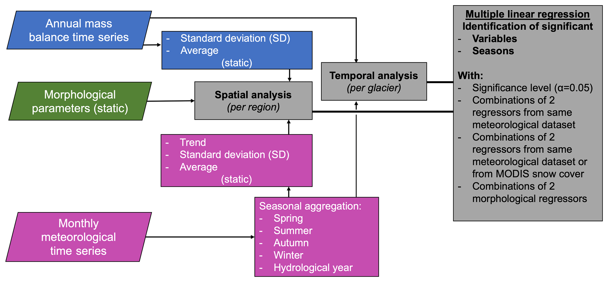
Figure 4 Workflow of spatial and temporal analyses using the mass balance estimates from Barandun et al. (2021a) and Hugonnet et al. (2021) and the meteorological data from the three different reanalysis products and MOD10CM snow cover (SC) as explained in the Data section. Focus in this study is to identify significant relationships rather than explain variance or other statistics. Therefore, identification of important variables and seasons is solely based on derived p values from multiple linear regression analyses. All significant correlations of a variable are used to produce the maps for the temporal analyses, and the reported relative importance in the spatial analysis is defined as the number of significant variables over the total number of tested variable combinations (see also Sect. 3).

3.1 Spatial correlation

The spatial correlation uses the derived average annual mass balances for each of the 1220 glaciers and provides results for either all of Tien Shan and Pamir or different regions divided according to two different classifications: HIMAP after Bolch et al. (2019) according (1) to main mountain range names (Fig. 1) and (2) to the mass balance variability found in Barandun et al. (2021a). The latter is determined using a k-means clustering with three fixed classes, where points are classified by minimizing their squared distance to the iteratively determined cluster centers (Pedregosa et al., 2011; Fig. 5). The k-means clustering is based on the standard deviation of the mass balance time series of Barandun et al. (2021a) and relies on an unsupervised classification that avoids a precise association of a class with, for example, a process. We arbitrarily chose a number of three clusters that would highlight the regions of high mass balance variability (hotspots) identified in Barandun et al. (2021a). The division is performed to determine whether different dominant predictors exist for these regions and, in general, to assess the effect of arbitrarily subdividing glaciers into different groups.

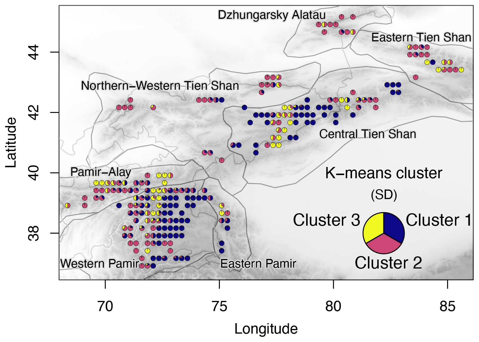
Figure 5 The k-means clusters according to mass balance variability (standard deviation – SD) for the 2000–2018 period from Barandun et al. (2021a). Classes represent glaciers with different variability.

We use either meteorological or morphological parameters as predictors. For meteorological predictors, we use the calculated average, standard deviation, and trend or tendency (derived slope from a temporal regression), each for the different seasons (spring, summer, autumn, winter) and the entire hydrological year (October–September) (Fig. 4). As static morphological predictors, we include the variables latitude, longitude, slope over the glacier tongue, median elevation, aspect, and glacier area from the RGI and debris cover from Scherler et al. (2018a). For aspect, we use the sine and cosine of the original values in the range between 0 and 360^∘ to obtain consistent value ranges in zonal and meridional directions. We showcase, additionally, any possible relationship with surge activity using separate histograms and boxplots where we simplify the complex information on surge activity provided in Guillet et al. (2022) as either (1) having experienced surge activity or (0) not during the 2000–2018 study period.

3.2 Temporal correlation

We run multiple linear regression analysis on the glacier mass balance time series per glacier to identify significant predictors over the time domain. Annual glacier mass balance time series represent the dependent variable; combinations of meteorological variables from individual reanalysis datasets represent the predictors. As this yields one result per glacier, we aggregate the results visually in the form of maps. We identify both significant variables and significant seasons to identify possible patterns and differences resulting from the use of a particular reanalysis or mass balance dataset.

4 Results

4.1 Comparison of reanalysis datasets

A comparison of the different reanalysis datasets is shown for precipitation in Fig. 3 and for temperature in Fig. A2. Only CHELSA provides a spatial resolution to resolve intra-mountain-range variability. Differences in precipitation amount and different trends exist independently of the spatial resolution (Fig. 3). However, for temperature, CHELSA is the temperature-conserving downscaled ERA5 product with matching trends and a correlation of 1 (Fig. A2i). For precipitation, CHELSA and ERA5 show deviating distribution patterns and trends, highlighting the nonlinear downscaling method (Fig. 3). The use of the datasets in their original spatial resolution in consecutive analyses allow for an assessment of how downscaling affects the correlation with mass balance data.

4.2 Spatial correlation

Despite a high number of significant correlations between mass balances and meteorological variables (70 %–90 %), the variability between the different datasets is high, leaving uncertain the interpretation on dominant drivers for Tien Shan and Pamir (Fig. 6). Obtained coefficients of determination (R²) are in the range of 5 % for all of Pamir and Tien Shan per variable and increase to up to 20 % for subregions (Fig. A3). When including remote sensing SC in addition to the reanalysis meteorological variables (T and P), SC represents about half the significant correlations. Without SC, a similar number of significant correlations indicates that SC explains a similar portion of the variance in mass balance but slightly more significantly than the variables from the reanalysis. The R² value remains low (Fig. A3). No dominant season can be identified in the analysis for Tien Shan or Pamir. Variability in the meteorological variables within each season and for the hydrological year are equally important (Fig. 6b and d).

Figure 6 Importance of (a, c) climatic variables, (b, d) season, and (e, f) morphological parameters for all of Tien Shan and Pamir. (a, b, e) Solid colors refer to MB_Barandunetal, and (c, d, f) semitransparent colors refer to MB_Hugonnetetal. Labels short and long refer to the periods 2000–2014 and 2000–2018, respectively. For the morphological analysis this refers to the glacier mass balance data.

Of the tested morphological parameters, 60 % to 70 % show a significant correlation with mass balances for all of Tien Shan and Pamir (Fig. 6e and f), and no individual morphological variable stands out as the most dominant one (Fig. 6). Each parameter is determined in 10 % of combinations as a significant predictor. Debris cover is not identified as an important variable in any case using mass balance datasets for either the short or long time period. This only changes in the regional division for some subregions (Fig. A4). However, depending on the mass balance estimates and subregion, the identified morphological parameters can change entirely. The mass balance distribution indicates no significant difference between surge- and nonsurge-type glaciers (Fig. A5). The small number of surge-type glaciers and the uneven distribution across the regions (Fig. A6) prevent a conclusive result.

Considering the different HIMAP regions (Bolch et al., 2019), the number of significant correlations between mass balance and meteorological variables varies strongly and depends on the mass balance dataset (Fig. 7). Overall, the total number of identified important variables is similar in both mass balance estimates. However, strong differences are apparent regarding which variable and temporal aggregation (seasons) is dominant. Likewise, the choice of a different reanalysis dataset results in different variable and temporal-aggregation importance. For example, a large number of significant correlations are present for Western Pamir and Northern–Western Tien Shan for MB_Barandunetal and for Central Tien Shan for MB_Hugonnetetal, whereas a medium number of significant correlations are present for Eastern and Central Tien Shan for MB_Barandunetal and for Western Pamir and Pamir-Alay for MB_Hugonnetetal (Fig. 7). For all other regions, the importance of meteorological variables is low and very variable from one dataset to another. For the majority of cases according to the HIMAP classification and for the entire region (Figs. 7, 6), the number of significant correlations is somewhat higher for the more highly spatially resolved CHELSA time series than for ERA5, despite CHELSA being based on ERA5 data as input. However, using the division according to the k-means clusters, this effect is not perceived (Fig. 8).

Snow cover increases the total number of significant correlations only for Central Tien Shan for MB_Barandunetal and for Eastern Tien Shan, Pamir-Alay, and Western and Eastern Pamir for MB_Hugonnetetal, despite contributing to at least half the significant combinations for most regions. For all other regions, T and P provide more significant correlations when SC is not considered. Combinations with SC barely show significant correlations in Eastern Pamir and Dzhungarsky Alatau (Fig. 7). Thus, incorporation of SC does not notably increase the number of significant correlations overall. Instead, a shift of important variables from P and T to SC occurs. This distinct shift from P and T to SC suggests that potential collinearity does not bias the general outcome.

We found clearly more significant combinations including P than those including T for Western Pamir and Pamir-Alay. T seems more significant for Eastern and Northern–Western Tien Shan and, to some degree, for Central Tien Shan. For Dzhungarsky Alatau, the results vary strongly between the different datasets, preventing a conclusion on the dominance of one of the meteorological variables. For Western Pamir and Eastern Tien Shan, winter and spring changes contribute to most of the significant combinations. The autumn season for Pamir-Alay and the summer and autumn seasons for Central and Northern–Western Tien Shan show the most significant correlations. For Eastern Pamir and Dzhungarsky Alatau, the different seasons contribute nearly equally to the number of significant combinations.

Besides the importance of the meteorological variables, the morphological-parameter importance is relatively high for Western Pamir (approx. 50 %; Fig. A4). However, no dominant morphological parameter could be identified, and variability across the different HIMAP regions and for the different mass balance estimates is high (Fig. A4). The only region in which both morphological and meteorological parameters show a high frequency of significant correlations is Western Pamir. In contrast, for Dzhungarsky Alatau and Eastern Pamir, none of these two categories of parameters show a high number of significant correlations with any of the mass balance estimates.

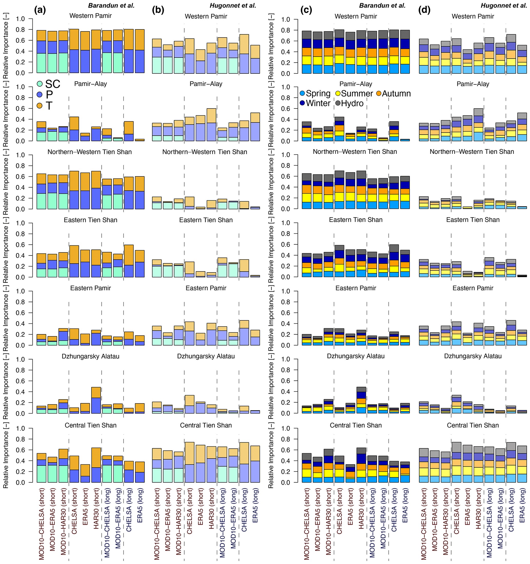
Figure 7 Importance of (a, b) meteorological variables and (c, d) seasons as the number of significant correlations identified using mass balance estimates from Barandun et al. (2021a) (solid color) and from Hugonnet et al. (2021) (semitransparent color) for the HIMAP regions. Labels short and long refer to the periods 2000–2014 and 2000–2018, respectively.

In contrast to the results for the regional HIMAP classification, a high number of significant correlations is always present within the k-means-derived hotspot regions of different mass balance variabilities (Fig. 8a and b). We found significant correlations for over 80 % of meteorological variables in cluster 1, slightly fewer in cluster 3 (60 %–80 %), and the lowest number, with high variability depending on the meteorological dataset used, for cluster 2 (40 %–70 %). Including SC did not increase the overall number of significant combinations for any of the three clusters, but this is the most important (relative highest number of correlations) variable for clusters 1 and 3. For cluster 1 (mainly positive and more balanced hotspot and low mass balance variability in MB_Barandunetal), P seems slightly more important than T; for cluster 2 (average mass balance with low variability, mainly along western/northwestern margins) T is dominant, and SC shows the lowest number of significant correlations compared with that of the other clusters; for cluster 3 (negative hotspot and high mass balance variability in MB_Barandunetal), T is slightly more dominant (Fig. 8).

For cluster 1, no clear dominance of either season is visible (Fig. 8c and d). In contrast, for clusters 2 and 3, some dominant seasons are apparent although dependent on the mass balance dataset. Generally, a more even distribution in seasonal importance is present for MB_Hugonnetetal than for MB_Barandunetal. The highest variability of dominant seasons was found for cluster 2 based on the reanalysis dataset used, with especially strong variability in the importance of spring and winter. Regarding the two mass balance estimates, MB_Barandunetal shows dominance in summer and autumn, while MB_Hugonnetetal shows dominance in winter and spring. The morphological variables show fewer significant correlations than the meteorological variables, especially for MB_Barandunetal in clusters 2 and 3 (Fig. A4).

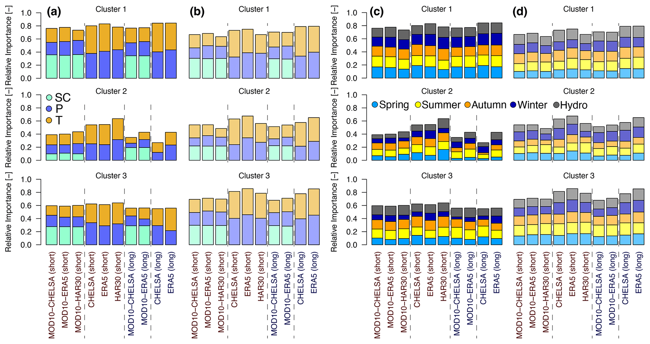
Figure 8 Same information shown in Fig. 7 but with glaciers aggregated according to similar glacier mass balance standard deviations (k-means clusters) found in Barandun et al. (2021a).

4.3 Temporal correlation

The explanatory power of the meteorological variables for the glacier-wide mass balance time series per individual glacier is between 30 % and 50 % (Fig. A7). However, similar to the spatial analysis, regional and dataset-dependent differences are apparent.

The importance of the variables depends strongly on the dataset used, and our analyses led to opposing results using the different products. This not only concerns the different reanalysis products but also the different mass balance time series. As an example, for Pamir-Alay, SC is the dominant variable for MB_Hugonnetetal, whereas T and P are the more important ones for MB_Barandunetal. A similar discrepancy was found for the different reanalysis datasets (Fig. 9); for example, for MB_Hugonnetetal, the central and southern parts of western Pamir are dominated by T using the HAR dataset, by SC using ERA5, and by P using CHELSA. This discrepancy is even clearer when SC is excluded from the analysis and only T and P are used as predictors for the mass balance time series (Fig. A8).

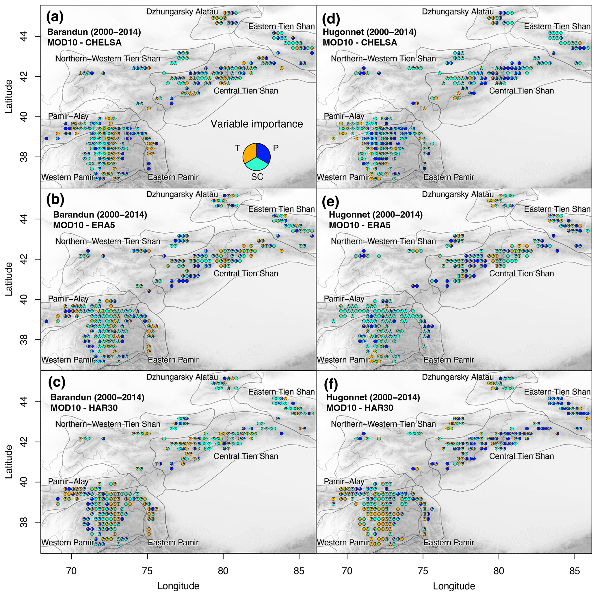
Figure 9 Importance of meteorological variables for the temporal analysis between annual mass balance estimates from (a–c) Barandun et al. (2021a) and (d–f) Hugonnet et al. (2021) and two meteorological variables from the different reanalysis datasets and SC.

Similarly, for the seasonal importance, results vary largely for the different glaciers depending on the dataset used and provide a more detailed view than that of the spatial analysis (Fig. 10). No consistency was found either for the same mass balance time series with different reanalysis products or for different mass balance time series with the same reanalysis product. When including SC, the pattern of variable importance becomes slightly more consistent in regions where SC replaces other variables as the most important variable (Fig. 10) without any apparent change in explained variance (Fig. A7).

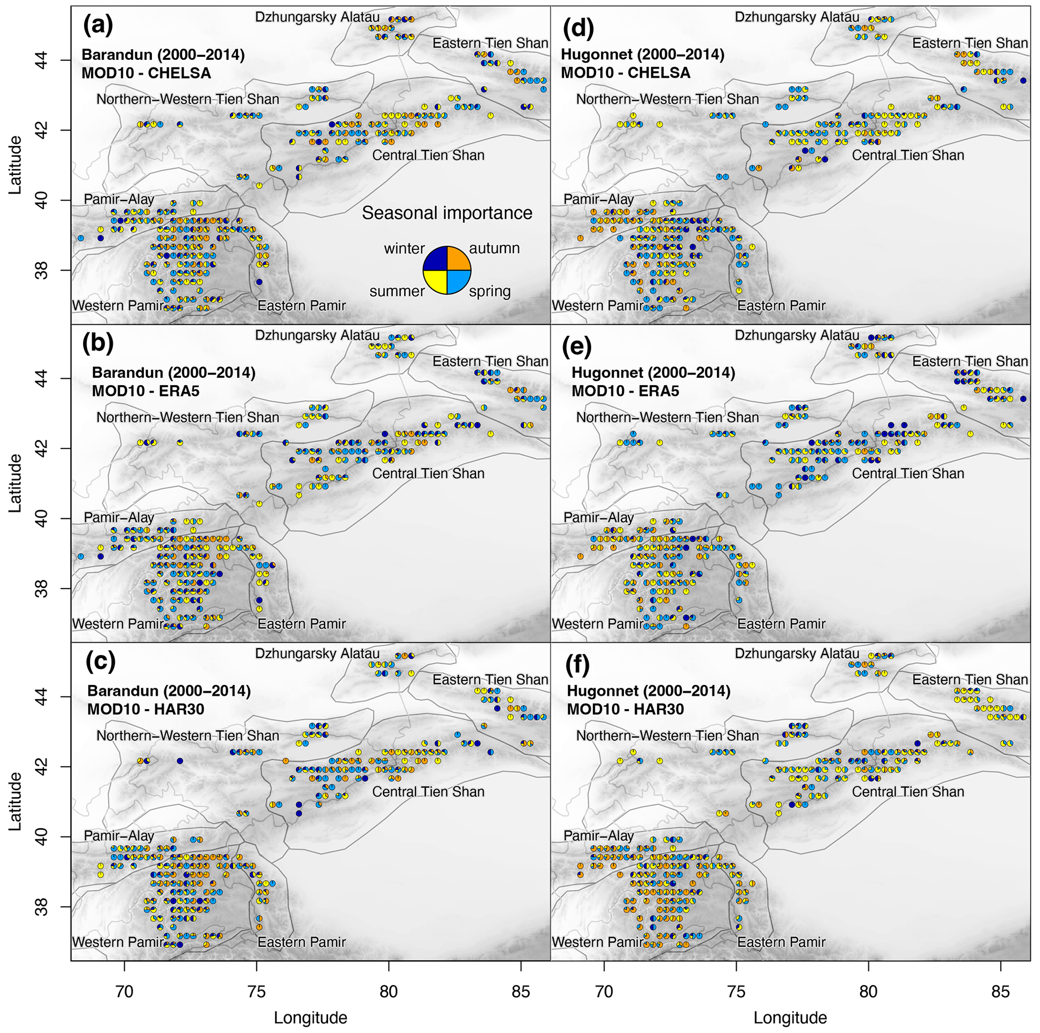
Figure 10 Seasonal importance from the temporal analysis between annual mass balance estimates from (a–c) Barandun et al. (2021a) and (d–f) Hugonnet et al. (2021) and two meteorological variables from the different reanalysis datasets; SC as indicated in the figure legends.

5 Discussion

Our temporal and spatial analyses (Sect. 4.1 and 4.3) offer radically different conclusions on the climatic drivers behind glacier mass balance response, independently of the mass balance estimate used or time period considered. According to our correlation analyses between the two mass balance estimates and different reanalysis products, in Pamir and Tien Shan, a clear identification of glacier-evolution-dominant drivers is impossible. Regional subdivision can significantly influence the outcome of a spatial analysis (Sect. 4.1), and aggregation or division of the total number of glaciers into regional clusters for comparison, although often required to summarize extensive study results (e.g., Brun et al., 2019), is somehow arbitrary. The use of temporal analysis based on annual mass balance time series can improve both the subregion definition and the aggregation process; however, this analysis depends strongly on the accuracy of the mass balance estimates at annual timescales, which are often highly uncertain, not observation based, or simply not available. In the present study, we discuss the uncertainty and danger of misinterpretations related to correlation analysis relying on individual data products.

5.1 Spatial resolution and downscaling

CHELSA is a processed and downscaled version of the ERA5 dataset. When using these two products, differences appear in the correlation analyses due to different spatial resolutions in the predictor variables; however, these differences only become striking when using the regional subdivision (Fig. 6). This might respond to a low number of data points with high mass balance variability within areas of encompassing meteorological grid cells, while the mass balance variability between the different encompassing grid cells in the regional subdivision is rather low. The nonlinearly downscaled precipitation of CHELSA (Fig. 3) compared with the conserving values for T (Fig. A2) can explain the higher number of significant correlations of this product compared with ERA5. As we use two predictor variables, the original P fields of CHELSA can change the significance of T. In the temporal analysis, the effect is even clearer, leading to partly opposing results (Figs. 9 and A8). We do not answer here how exactly any downscaling method can affect results, but we show that advanced downscaling methods (CHELSA's precipitation) can severely impact driver interpretation. Different outcomes can be expected depending on the downscaling technique used, adding subjectivity to the results.

5.2 Correlation analysis

Our results reveal a high number of significant correlations between T, P, and mass balance for the entire Pamir and Tien Shan region (Fig. 6), largely independent of the mass balance estimate or reanalysis product. The relative number of significant correlations remains similar when introducing SC, suggesting that the meteorological parameters from the reanalysis and SC relate similarly to the spatial variability in glacier mass balances.

When dividing glaciers regionally, the number of significant correlations between T, P, SC, and mass balance decreases, and the identified variables are shown to depend strongly on the datasets used (Figs. 7 and 8). The low number of significant correlations for certain subregions can respond to (1) data availability, (2) data quality and scale issues, and (3) process representation.

1. Due to the lower number of glaciers with mass balance time series available, especially for Eastern Pamir and Dzhungarsky Alatau, the robustness of the statistical analysis is reduced, making it difficult to find a significant correlation with the meteorological variables.

2. The meteorological variables used cannot represent on their own the relevant processes responsible for the mass balance variability. For example, at high elevations, the relevance of temperature and longwave radiation can decrease in favor of shortwave radiation, which could likewise explain lower numbers of significant correlations for T in Eastern Pamir, where the highest glaciers are located (Sicart et al., 2011; Yang et al., 2011). The larger changes in meteorological forcing needed for a glacier response in areas with lower mass balance sensitivity (regions with more continental climate regimes) are easier to capture in reanalysis than the small changes that can make glaciers react in areas with higher sensitivity (subcontinental regions). For example, small-scale processes (e.g., changes in pore space) close to the equilibrium line of altitude can change accumulation patterns to which such glaciers react sensitively (Kronenberg et al., 2022). This can explain the lower number of significant correlations found for more subcontinental settings. Such scale-related issues can also explain some of the contrasting patterns in the correlation analysis resulting from the different reanalysis products due to their different spatial resolution.

3. Changing mass balance variability, sensitivity, response times, or mass balance gradients and regimes can further complicate finding consistent relationships under climate change at a subregional scale. Based on station data, Wang et al. (2019) showed that subcontinental glaciers react mostly to air temperature variability, whereas continental glaciers, generally located at higher elevations, are sensitive to both air temperature and precipitation. Under ongoing climate change, glacier response to meteorological conditions undergo important changes due to changing mass balance sensitivity and variability (Azisov et al., 2022; Dyurgerov and Dwyer, 2000), partly related to a shift from continental to more subcontinental conditions, thus shifting the dependence on specific meteorological variables. Changes in mass balance gradient such as rotation (simultaneous increase of ablation with decreasing elevation and increase of accumulation with increasing elevation or vice versa) or parallel shifts of the mass balance gradients (simultaneous increased ablation and decreased accumulation or vice versa) have been observed for the region (Kronenberg et al., 2022; Dyurgerov and Dwyer, 2000; Azisov et al., 2022; Kuhn, 1980, 1984). Such shifts, in return, influence the mass balance sensitivity (Wang et al., 2017) and variability (Barandun et al., 2021a).

Our analysis reflects all of the above issues. Glaciers in cluster 2 (subcontinental climate regime) are more heterogeneously distributed spatially (Fig. 5), and this cluster shows the lowest number of significant correlations. In combination with the high variability within the datasets, our results suggest that glacier mass balance variability does not result from the investigated meteorological drivers for this cluster, suggesting that a similar mass balance variability is a response to different drivers within this cluster. Conversely, glaciers in clusters 1 (continental climate regime) and 3 (hotspots of mass balance variability) are much more aggregated spatially, and the investigated meteorological and morphological parameters better represent the subregional mass balance variability. At this point especially precipitation estimates are imprecise in general (Palazzi et al., 2013), as well as at the glacier scale as a result of, e.g., coarse resolution or insufficiently represented localized precipitation events such as orographic precipitation effects (Roe et al., 2003). What is responsible for the high variability within the data-scarce region of cluster 2 remains unclear. An interesting finding is the lower number of correlations when including SC for both mass balance estimates. This is especially pronounced for cluster 2 (Fig. 8), where a low fraction of variable combinations identifies SC in combination with MB_Barandunetal. This can indicate that a crucial meteorological component is missing in our analysis and that T and P estimates are a surrogate for a process not related to snow dynamics. For these cases, glacier response might be more related to radiation, physical snow properties (e.g., albedo, grain size), or the amount of snow, which in total are better represented by simply using T and P than with the qualitative information of SC. In contrast, a similar number of correlations would indicate that T and P explain processes similarly to SC.

Our results indicate a tendency for stronger summer and autumn influence along the northwestern margin and, to some extent, for the negative hotspot that could be linked to either summer snowfall events or changing melt rates due to changes in air temperature. This contrasts the importance of autumn to spring for the positive mass balance anomalies in Western Pamir and Central Tien Shan, which can relate to changing snow cover dynamics and/or changes in solid–liquid precipitation ratios, supported by the high number of significant correlations including P. However, we have not identified a strong seasonal importance of the meteorological variables in our spatial analysis (Figs. 7 and 8).

5.3 What are the dominant climatic drivers?

Our results show a heterogeneous picture of dominant variables and seasons from 2000 to 2014 (2018), strongly dependent on the choice of datasets. An interpretation based on an individual dataset can contradict a different interpretation based on another set of data, both of them well supported by the literature. Here we show two somewhat contradicting but plausible interpretations of meteorological drivers for glacier mass balance changes based on the results of our temporal and spatial analysis to highlight the persistent difficulty to shed light onto the glacier–climate interaction in a heterogeneous and data-sparse region such as Central Asia.

5.3.1 Analysis I: HAR dataset and MB_Barandunetal

Mass balance data are based on MB_Barandunetal, and all drivers refer to the identified HAR meteorological variables in our results (Fig. 11a).

Air temperature increased by about 0.1 to 0.2 ^∘C per decade in Tien Shan from 1960 to 2007 (Aizen et al., 1996; Kutuzov and Shahgedanova, 2009; Kriegel et al., 2013). Air temperature is the dominant driver for the mass balance of most glaciers located in Tien Shan, most dominantly in spring and autumn (Fig. 9). In Eastern Tien Shan and Dzhungarsky Alatau, air temperature and snow cover in spring and summer are the dominant drivers identified for the high mass loss (Figs. 9c, 10c). This might relate to a pronounced snow cover decrease in Eastern Tien Shan (Notarnicola, 2020) as a result of increased air temperatures causing faster snow depletion in late spring and early summer. In line with that, Sakai and Fujita (2017) concluded that climatic settings were represented by the three factors of (i) summer temperature, (ii) temperature range, and (iii) summer precipitation ratio, which are the most important factors for mass balance variability.

Although Haag et al. (2019) reported a slight positive trend in summer, winter, and autumn precipitation for Tien Shan from precipitation anomaly time series for the period 1950 to 2016 for all of Central Asia, our analysis did not identify these changes as individually dominant drivers for mass balances at the regional scale (Fig. 6a and b). More locally, increasing spring and summer precipitation in combination with an autumn and summer cooling in Central Tien Shan (e.g., Li et al., 2022) aligns with the cluster of close-to-zero and slightly positive mass balances.

The positive mass balance anomaly in Barandun et al. (2021a) can be explained by a positive snow cover change matching its location (Notarnicola, 2020). A localized temperature decrease in Central Tien Shan in summer increases the frequency of solid-precipitation events that lower melt rates due to a positive albedo effect of fresh snow (e.g., Kronenberg et al., 2016). This is reflected by the importance of a changing snow cover and the seasonal importance from spring to autumn (Figs. 10c, 9c), in line with the heterogeneous and sharply contrasting snow cover changes reported by Notarnicola (2020). The neighboring negative mass balance anomaly in Central Tien Shan reflects the air temperature and spring importance, with a sharp decrease in snow cover duration (Notarnicola, 2020).

Mass balances of the glaciers located in the eastern part of Western Pamir can respond to the north-to-south gradient (summer cooling for northern Pamir and warming trend for southern Pamir) reported by Knoche et al. (2017). These mass balances are therefore mainly driven by air temperatures (Fig. 9c).

Despite the nonsignificant precipitation trends for all of Pamir (Pohl et al., 2017), winter precipitation has increased since 1950 in Pamir-Alay (Haag et al., 2019; Kronenberg et al., 2021). Winter precipitation changes, however, play a subordinate role in the glacier mass balance of Pamir-Alay, whereas spring and summer changes dominate (Figs. 9c, 10c). Figures 9c and 10c suggest that only glaciers with lower negative mass balances show a relation with winter precipitation, whereas the driver for the mass balance of most glaciers in the region is temperature (also snow cover changes in the eastern part of Pamir-Alay).

5.3.2 Analysis II: ERA5 dataset and MB_Hugonnetetal

Mass balance data are based on MB_Hugonnetetal, and all drivers refer to the identified ERA5 meteorological variables in our results (Fig. 11b).

Air temperature increased by about 0.1 to 0.2 ^∘C per decade in Tien Shan from 1960 to 2007 (Aizen et al., 1996; Kutuzov and Shahgedanova, 2009; Kriegel et al., 2013). However, precipitation and snow cover are more important drivers than temperature for the mass balance of glaciers located in all of Tien Shan (Figs. 7, 9). Whilst in the southwestern part, spring is the most important season, winter is more important in the northeastern part of Tien Shan, where glacier mass loss is especially pronounced (Fig. 10e). In the Eastern Tien Shan, decreasing precipitation and snow cover are the main drivers identified for the negative mass balances (Fig. 9e). For Dzhungarsky Alatau, however, mass loss seems mainly driven by temperature and snow cover (Fig. 9e).

Haag et al. (2019) reported a slightly positive trend in summer, winter, and autumn precipitation for Tien Shan that influences the close-to-zero and slightly positive mass balances at the southern margin of Tien Shan. This agrees with the increase of snow cover fraction reported in Notarnicola (2020).

At the western margin of Central Tien Shan, less negative mass balances are in line with reported positive precipitation changes (Aizen et al., 1996; Kutuzov and Shahgedanova, 2009; Kriegel et al., 2013). Therefore, the main drivers seem to be precipitation and snow cover in spring and summer (Figs. 9e, 10e).

Positive mass balances of the glaciers located in the western margin of Pamir-Alay can be related to increased snow cover (Notarnicola, 2020, reported a longer snow cover duration from 2000 to 2018) and decreasing temperatures during the transition from winter to summer; this allows snow to persist longer and an earlier snowfall in autumn to shorten the ablation season, acting favorably on the glacier mass balances.

Haag et al. (2019) showed that, despite the nonsignificant trend of annual precipitation amounts, summer precipitation had significantly increased by around 5 mm per decade for Western and Eastern Pamir. Summer and early-autumn precipitation represents the most important driver for the positive mass balances in Eastern Pamir, in combination with an important summer cooling reported for nearby Karakorum during the past decades (Fowler and Archer, 2006; Mölg et al., 2014; Forsythe et al., 2017). Summer snowfall, on the one hand, acts directly as a mass contributor and, on the other, lowers melt rates due to a positive albedo effect (e.g., Kronenberg et al., 2016); de Kok et al. (2020) suggest that low temperature sensitivities in combination with an increase in snowfall, largely due to increases in evapotranspiration from irrigated agriculture, explain the positive mass balances in this region.

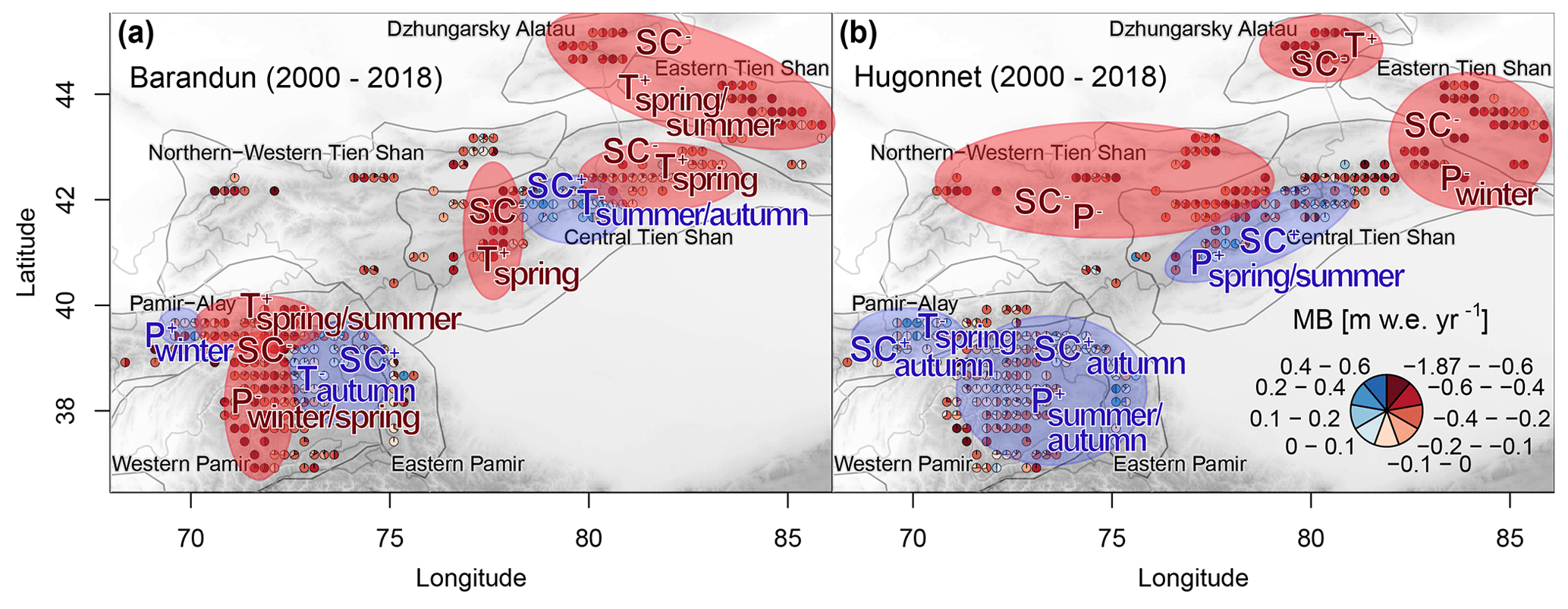
Figure 11 Summary of dominant drivers found for (a) Analysis I and (b) Analysis II. P denotes precipitation, T denotes air temperature, and SC denotes snow cover. A negative sign indicates a decrease, and a positive sign indicates an increase. Effects associated with more positive mass balances, such as an increase in precipitation and snow cover or a decrease in temperature, are highlighted in blue and vice versa in red.

5.4 Implications from the spatial and temporal analyses

The resulting importance of the seasons and meteorological variables from the temporal and spatial analyses is strongly dependent on the dataset used, sometimes suggesting even a contradicting relationship with glacier response. Clear nonclimatic drivers cannot be identified. Derived interpretations (from Analysis I and Analysis II) align with other reported findings in these regions, as shown in Sect. 5, rendering the interpretation and analysis even more difficult. Available time series fall short of robust evidence in the correlation analysis due to high meteorological and mass balance variability compared with rather slight trends and tendencies in these time series. Using different meteorological and mass balance estimates, our study highlights in all cases a highly complex glacier response to climate variability and change. The current lack of sufficiently detailed and qualitatively satisfying data prevents elucidating the complex relationship between glacier mass balance and climatic drivers in Tien Shan and Pamir.

A lack of regional-wide systematic cryospheric and atmospheric monitoring limits the validation of the available datasets for scientific applications, resulting in an elevated uncertainty for mass balance modeling and interpretation on the underlying processes of glacier response to climate change. We cannot rate the different products. Cryological, hydrological, and meteorological monitoring at high elevation throughout the different subregions of Tien Shan and Pamir needs to improve for a better understanding of glacier response to climate change. In several subregions, no glaciers are systematically monitored (Barandun et al., 2020), in situ snow monitoring is not established, and hydrological monitoring is very limited (Unger-Shayesteh et al., 2013; Hoelzle et al., 2019). Meteorological measurements are underrepresented at high elevation and, for certain subregions, completely lacking (Unger-Shayesteh et al., 2013; Sorg et al., 2012). Most existing data are inaccessible. The needed long-term systematic monitoring of the different components of the water cycle often lacks financial support, know-how, and personpower (Hoelzle et al., 2019; Barandun et al., 2020). When using only one specific dataset, differences in reanalysis products and elevated uncertainties tied to the available annual mass balance time series for Tien Shan and Pamir underpin the ambiguity in the interpretation of the results of a correlation analysis. As highlighted by the two scenarios presented in Sect. 5, any derived understanding of glacier–climate interactions depends strongly on the dataset used. When a thorough quality assessment of the different reanalysis products for further application cannot be assured, the limitations of these datasets cascade into an increase of uncertainties. This especially affects the modeling of future glacier response, hydrological modeling, and the equifinality problem related to too many unknowns in the cryohydrological cycle (e.g., Beven, 2006; Farinotti et al., 2015) or reconstruction of glacier mass change without a good calibration dataset. Traditionally, many studies have been based on a single reanalysis dataset, used either for bias correction or directly as model input, and direct calibration data are generally limited to a few individual locations, insufficient for regional applications. Remote sensing can partly bridge the gap in observational data, and progress has been made to increase temporal resolution of geodetic mass balance estimates (Beraud et al., 2022). Furthermore, integration of different and sometimes unconventional datasets with information on the atmospheric conditions, the earth surface energy balance, glacier response, and other water storage changes (Farinotti et al., 2015; Pohl et al., 2017; Naegeli et al., 2022; Key et al., 1997) is valuable for assessing and possibly quantifying uncertainties related to the presented datasets and, eventually, rating their quality. Modern downscaling techniques such as those provided in Fiddes and Gruber (2014, 2012) facilitate the inclusion of small-scale topographic effects. Standardizing sophisticated downscaling methods can improve the spatial representations of the reanalysis datasets. Despite potential improvements (remote sensing, Beraud et al., 2022; integration of unconventional datasets, Farinotti et al., 2015; Pohl et al., 2017; Naegeli et al., 2022; Key et al., 1997; and modern downscaling technics, Fiddes and Gruber, 2014, 2012), we recommend not relying on a single product for either correlation analysis or cryohydrological modeling.

6 Conclusions

The extreme scarcity of in situ observations for both meteorological variables and glacier mass balance in Central Asia leaves much space for different interpretations regarding how glaciers may evolve in this region within a changing-climate scenario. As a result, water availability assessment for the growing population is uncertain. Our study shows that even supposedly similar datasets such as ERA5 and its CHELSA derivative lead to different and partly contradicting assumptions of drivers for mass balance variability. The ease of use and great availability of datasets such as ERA5 might lead to a one-sided use of certain datasets to the detriment of those less comprehensive but more thoroughly validated ones such as HAR v1.4, whose shortcomings are better known. Our study points to a trend in which apparent but false consistencies across studies using a single dataset can largely relate to the chosen dataset rather than to the processes or involved environmental variables. We showcase how important variables change with the use of the two different mass balance datasets even though said datasets agree at the regional scale; differences at individual glacier scale are stark. Regionally aggregated mass balance estimates are useful for summarizing and reporting results, e.g., following the HIMAP classification or our glacier mass balance (MB_Barandunetal) standard-deviation-based k-means clusters. However, derived interpretations about important drivers carry a large subjective and arbitrary aspect, as these interpretations can change significantly based on the chosen clustering. This effect is largely remediated in the temporal analysis, where each glacier–meteorological relationship is preserved. Such analysis, however, requires mass balance time series that geodetic methods cannot provide by default and with the trade-off of increasing uncertainty at short timescales.

The aspects, from highest to lowest impact, for deriving conclusive results are

• differences in meteorological data

• differences in mass balance data

• regional classifications and aggregations.

In the present work, we cannot reach a conclusion about the driving meteorological and morphological variables of mass balance variability in Tien Shan and Pamir. In this data-scarce region, where meteorological or mass balance datasets cannot be rigorously validated with ground truth data, the only honest option from a scientific point of view is to “suggest” rather than “state” the existence of found relationships and inferred dependencies.

Appendix A

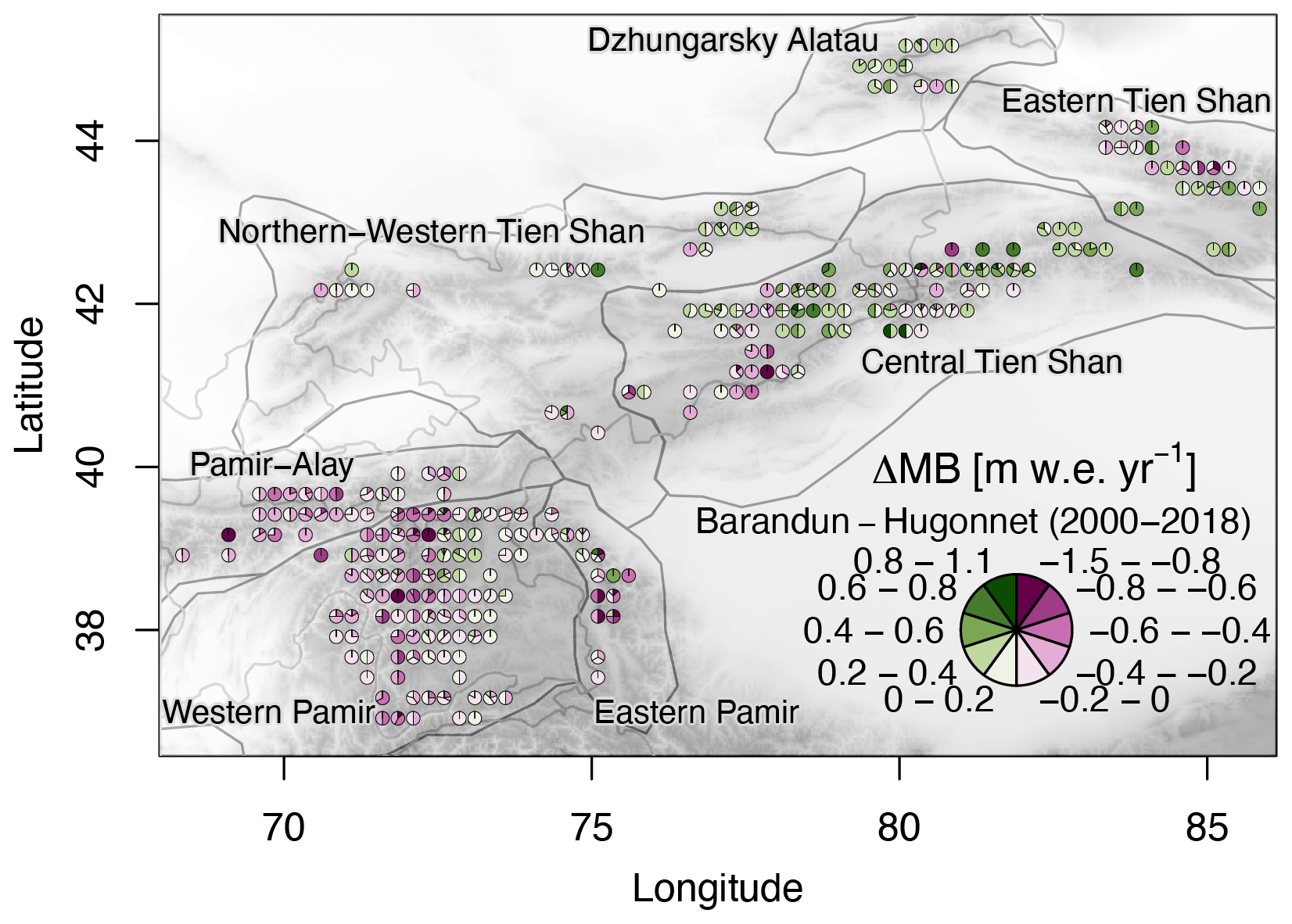
Figure A1 Difference in mean annual glacier mass balance between Barandun et al. (2021a) and Hugonnet et al. (2021) for the period 2000–20018. Estimates from Hugonnet et al. (2021) only include the glaciers for which the transient-snowline-constrained modeling of Barandun et al. (2021a) provides estimates. The pie charts aggregate values per glacier into classes and the relative class frequencies. Pie charts are not scaled to glacier area.

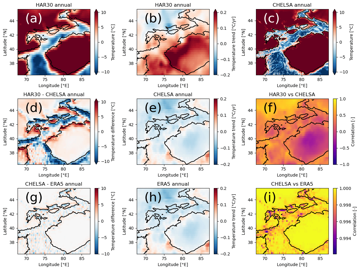
Figure A2 Mean annual temperature for (a) HAR30 and (c) CHELSA. Trends for (b) HAR30, (e) CHELSA, and (h) ERA5. Differences between the datasets (d) HAR30 and CHELSA and (g) CHELSA and ERA5 and the correlation between (f) HAR30 and CHELSA and (i) CHELSA and ERA5. CHELSA and ERA5 are spatially resampled to the resolution of HAR30 for the differences and correlation. Note the different scale for the correlation in (i). Black outlines correspond to 2000 m a.s.l. altitude.

file

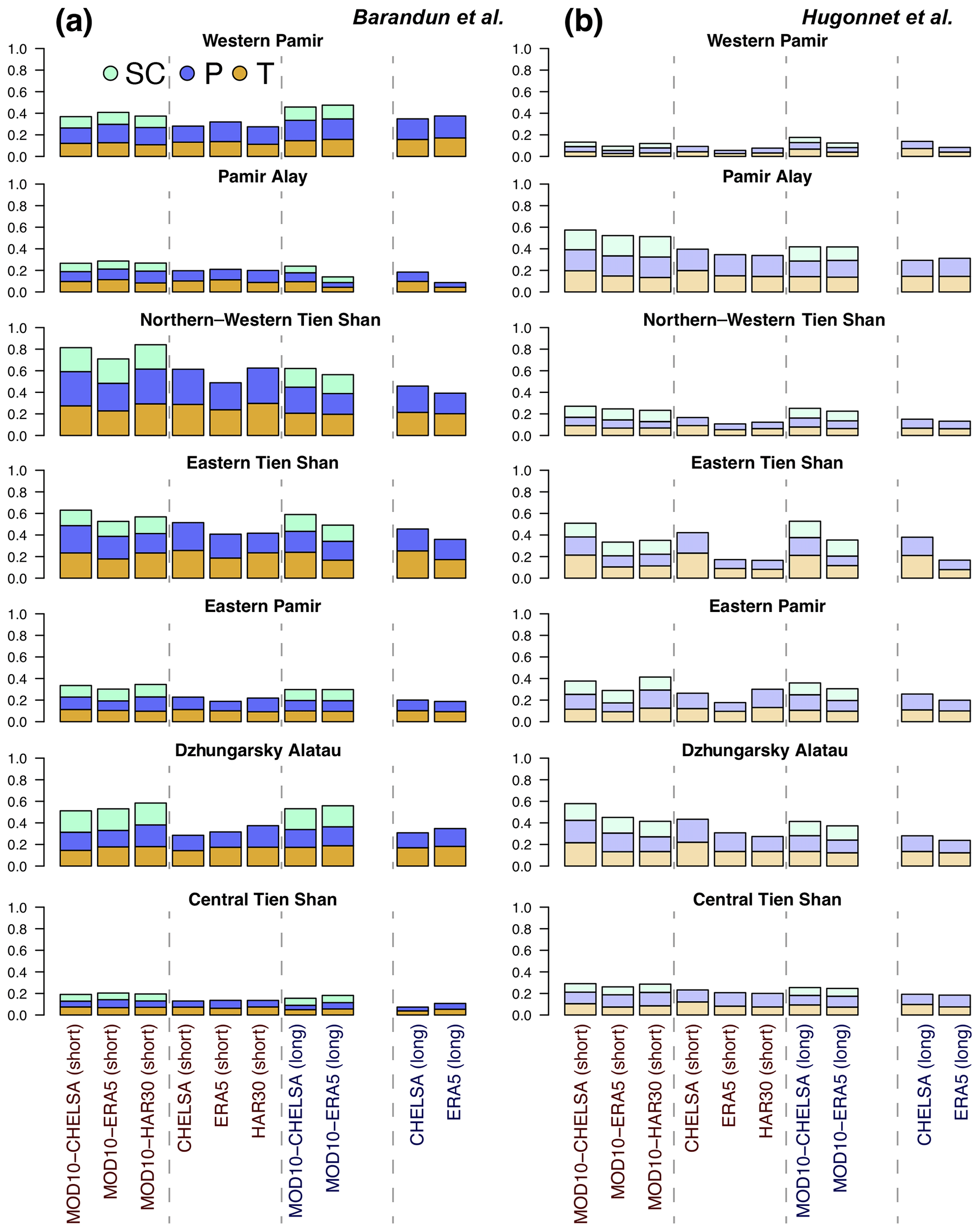
Figure A3 Coefficient of determination (R²) for variables in the spatial analysis. The shown R² is the average for all variable combinations in which the displayed meteorological variable (SC, P, T) is contained. Mass balance estimates of (a) Barandun et al. (2021a) and (b) Hugonnet et al. (2021).

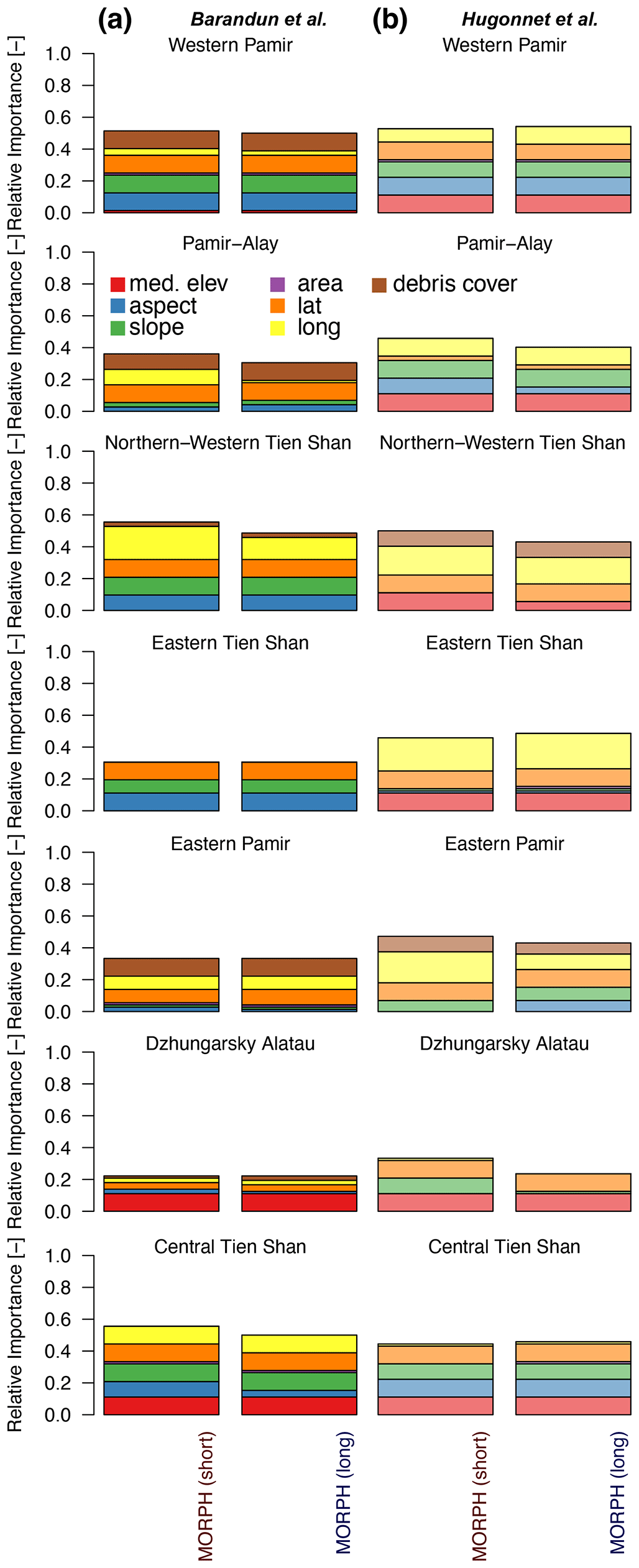
Figure A4 Frequency of significant morphological variables for the HIMAP regions and for the two mass balance estimates by (a) Barandun et al. (2021a) and (b) Hugonnet et al. (2021).

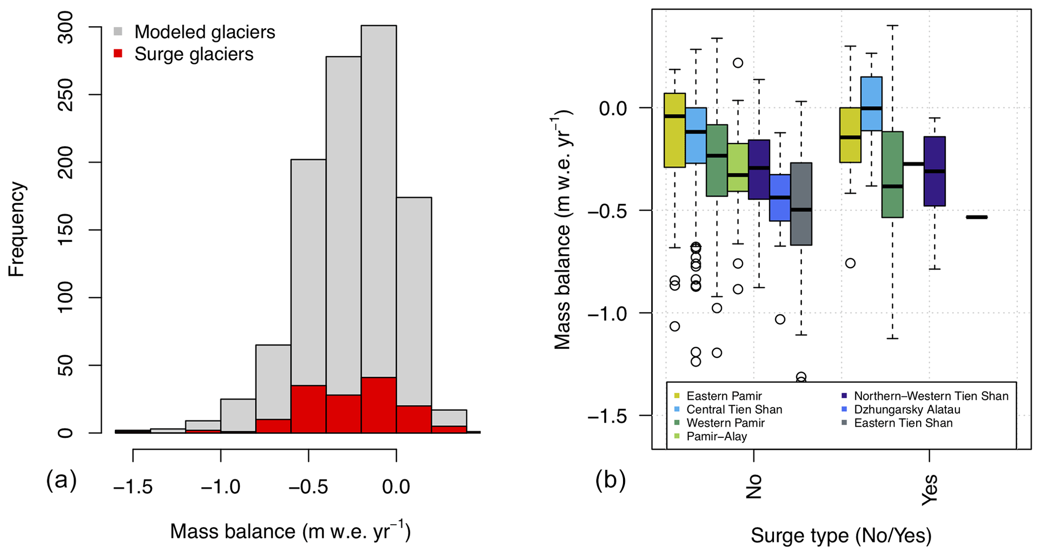
Figure A5 Distribution of surge-type glaciers and mass balance range (a) of all glaciers and (b) for the HIMAP regions. The regional comparison shows that no systematic difference was found between the relationship of surge- and nonsurge-type glaciers with mass balance.

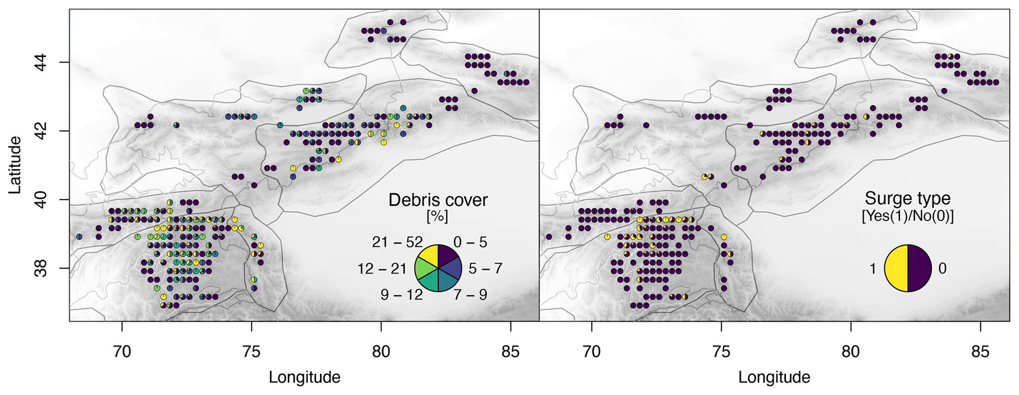
Figure A6 Surge-type glacier (Guillet et al., 2022) and debris cover (Scherler et al., 2018a) distribution in Tien Shan and Pamir.

Figure A7 Coefficient of determination (R²) of temporal analysis between annual mass balance estimates from Barandun et al. (2021a) and Hugonnet et al. (2021) and two meteorological variables from the different reanalysis datasets as indicated in the figure legends. Upper two panels without and lower two panels including snow cover.

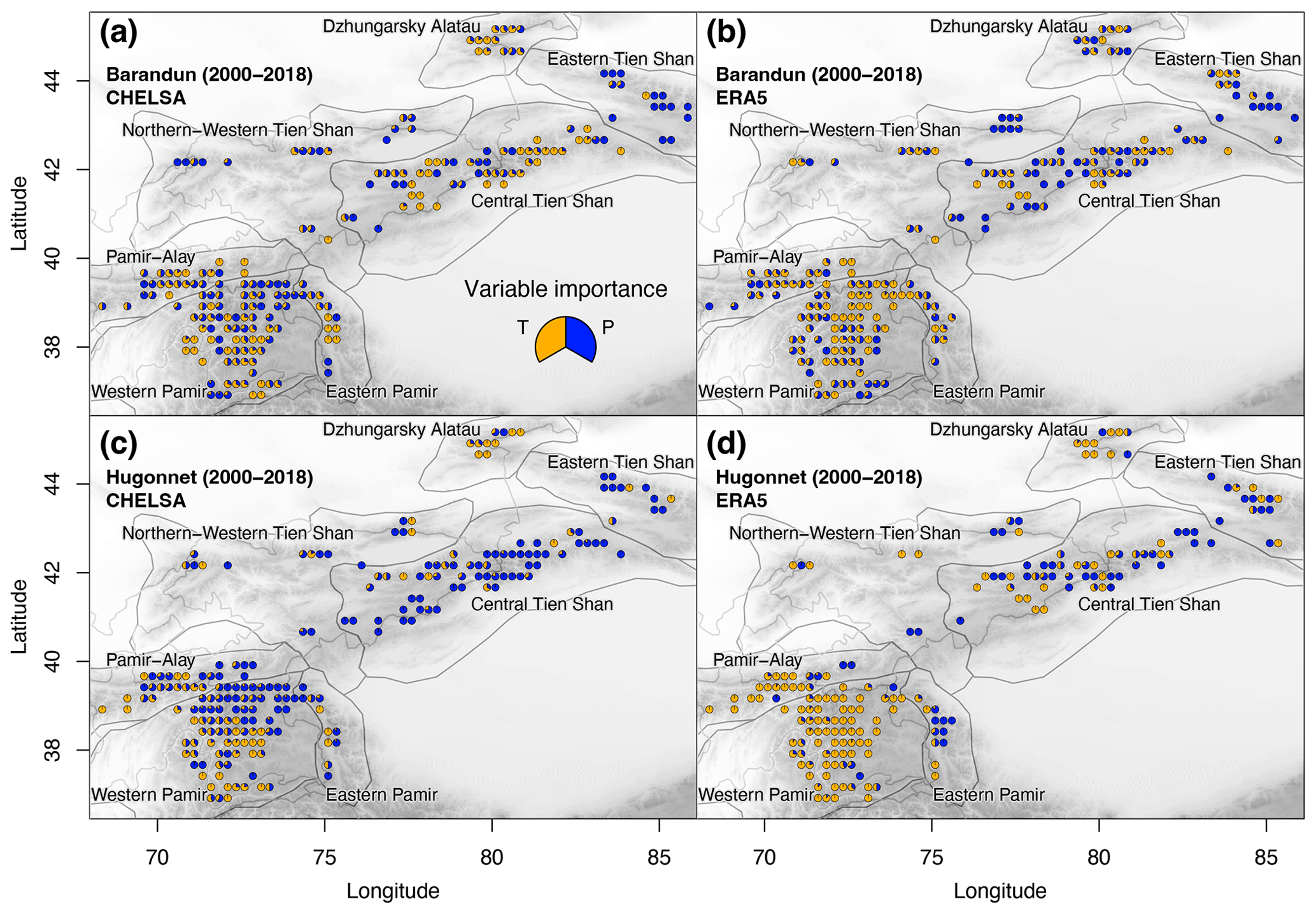
Figure A8 Importance of meteorological variables for temporal analysis between annual mass balance estimates from (a, b) Barandun et al. (2021a) and (c, d) Hugonnet et al. (2021) and two meteorological variables (T and P) from the different reanalysis datasets.