the Creative Commons Attribution 4.0 License.
the Creative Commons Attribution 4.0 License.
 | 10 Mar 2023
Exploring the role of snow metamorphism on the isotopic composition of the surface snow at EastGRIP
Romilly Harris Stuart
Anne-Katrine Faber
Sonja Wahl
Maria Hörhold
Sepp Kipfstuhl
Kristian Vasskog
Melanie Behrens
Alexandra M. Zuhr
Hans Christian Steen-Larsen
Stable water isotopes from polar ice cores are invaluable high-resolution climate proxy records. Recent studies have aimed to improve our understanding of how the climate signal is stored in the stable water isotope record by addressing the influence of post-depositional processes on the isotopic composition of surface snow. In this study, the relationship between surface snow metamorphism and water isotopes during precipitation-free periods is explored using measurements of snow-specific surface area (SSA). Continuous daily SSA measurements from the East Greenland Ice Core Project site (EastGRIP) during the summer seasons of 2017, 2018 and 2019 are used to develop an empirical decay model to describe events of rapid decrease in SSA linked to snow metamorphism. We find that SSA decay during precipitation-free periods at the EastGRIP site is best described by the exponential equation , and has a dependency on wind speed. The relationship between surface snow SSA and snow isotopic composition is primarily explored using empirical orthogonal function analysis. A coherence between SSA and deuterium excess is apparent during 2017 and 2019, suggesting that processes driving change in SSA also influence snow deuterium excess. By contrast, 2018 was characterised by a covariance between SSA and δ18O highlighting the inter-annual variability in surface regimes. Moreover, we observed changes in isotopic composition consistent with fractionation effects associated with sublimation and vapour diffusion during periods of rapid decrease in SSA. Our findings support recent studies which provide evidence of isotopic fractionation during sublimation, and show that snow deuterium excess is modified during snow metamorphism.
- Article
(7110 KB) - Full-text XML
- BibTeX
- EndNote


The traditional interpretation of stable water isotopes in ice cores is based on the linear relationship between local temperature and first-order parameters δ18O and δD of surface snow on ice sheets (Dansgaard, 1964). Accurate reconstruction requires consideration of precipitation intermittency (Casado et al., 2020; Laepple et al., 2018), past variations in ice-sheet elevation (Vinther et al., 2009), sea ice extent (Faber et al., 2017; Sime et al., 2013), and firn diffusion (Johnsen et al., 2000; Landais et al., 2006; Holme et al., 2018), which influence the water isotopic composition in ice cores. The second-order parameter deuterium excess (d-excess) is defined by the deviation from the near-linear relationship between δ18O and δD which is driven by non-equilibrium (kinetic) fractionation (d-excess = δD O). d-excess in ice cores is understood to reflect moisture source conditions (Dansgaard, 1964; Merlivat and Jouzel, 1979; Johnsen et al., 1989) and changes in moisture source region (Masson-Delmotte et al., 2005), and can be modified during snow crystal formation in supersaturated clouds (Ciais and Jouzel, 1994; Sodemann et al., 2008). Recent studies have documented isotopic composition change in the surface snow during precipitation-free periods (Steen-Larsen et al., 2014; Ritter et al., 2016; Casado et al., 2018; Hughes et al., 2021), linked to synoptic variations in atmospheric water vapour composition and subsequent exchange with the surface snow (Steen-Larsen et al., 2014; Ritter et al., 2016; Madsen et al., 2019; Hughes et al., 2021; Wahl et al., 2021; Casado et al., 2021). Post-depositional processes at the surface involve additional kinetic effects adding complexity to the interpretation of d-excess (Hughes et al., 2021; Casado et al., 2021). Here we focus on processes influencing the isotopic composition of the surface snow after deposition while exposed to surface processes, and concentrate on the second-order parameter d-excess due to its sensitivity to kinetic effects.
After deposition, snow grains undergo structural changes known as “snow metamorphism”, which is active at the surface and at greater depths, depending on temperature (gradient) conditions (Colbeck, 1983; Pinzer and Schneebeli, 2009). Surface snow metamorphism is initially driven by a reduction in the snow–air interface to reach thermodynamic stability (Colbeck, 1980; Legagneux and Domine, 2005). The snow–air interface can be described by the widely used parameter snow-specific surface area (SSA), which is dependent on optical grain radius and density of ice (SSA = ) (Gallet et al., 2009) and can be used as an indicator for snow metamorphism (Cabanes et al., 2002, 2003; Legagneux et al., 2002). Freshly deposited snow has a high SSA which decreases with time under both isothermal (<10 ∘C m−1) and temperature gradient (>10 ∘C m−1) conditions within the snow (Cabanes et al., 2002; Legagneux et al., 2004; Domine et al., 2007; Genthon et al., 2017). A decrease in SSA in dry snow is predominantly the result of water vapour transfer among grains, with smaller grains feeding the growth of larger grains (Legagneux et al., 2004; Flin and Brzoska, 2008; Sokratov and Golubev, 2009; Pinzer et al., 2012). Ventilation by wind can accelerate SSA decrease by enhancing water vapour transfer rates (Picard et al., 2019). Under natural conditions, SSA decrease is driven by a combination of these processes depending on surface conditions (Cabanes et al., 2003; Pinzer and Schneebeli, 2009), each potentially modifying the isotopic composition of the snow (Ebner et al., 2017).
Models can provide a quantitative description of SSA decrease after deposition. Previous studies have proposed SSA decay models using a combination of field measurements and controlled laboratory experiments (Cabanes et al., 2002, 2003; Legagneux et al., 2003, 2004; Flanner and Zender, 2006; Taillandier et al., 2007). Exponential models are documented to produce the best fit to in situ SSA decay data given that they can account for temperature effects under various wind conditions while being simple in their formulation (Cabanes et al., 2003). A subsequent physical-based model was defined by Legagneux et al. (2004) to describe SSA decay based on grain growth theory, which was then further developed by Flanner and Zender (2006), who defined parameters based on surface temperature, temperature gradient and snow density. Existing SSA decay models have rarely been applied to polar ice sheet surface snow (Linow et al., 2012; Carmagnola et al., 2013). Conditions for surface snow on polar ice sheets are not necessarily comparable to other alpine and arctic regions due to negligible melt and the high-latitude radiation budget. Moreover, while continuous surface SSA measurements exist from Antarctica (Gallet et al., 2011, 2014; Picard et al., 2014), those from Greenland focus on the depth evolution of SSA (Linow et al., 2012; Carmagnola et al., 2013). Continuous datasets of daily SSA and corresponding isotopic composition measurements from the accumulation zone of the Greenland Ice Sheet are required for understanding the influence of surface snow metamorphism on surface energy budget (Picard et al., 2012), and for the interpretation of ice core water isotope records (Casado et al., 2021; Wahl et al., 2022). In this study we focus on the latter, which is of particular importance owing to observations of isotopic fractionation during snow metamorphism documented in laboratory studies (Ebner et al., 2017) and field experiments (Casado et al., 2021; Hughes et al., 2021; Wahl et al., 2021). Nonetheless, few studies have focused on the direct relationship between physical snow properties, such as SSA, and post-depositional changes in isotopic composition.
In this paper, the aim is to explore the behaviour of surface snow metamorphism on polar ice sheets using daily SSA measurements from northeast Greenland during summer, and to compare the change in physical properties with the isotopic composition measurements. The primary focus is to document events where changes in SSA occur rapidly over a number of precipitation-free days, which we use as a proxy for snow metamorphism. Events of rapid SSA decrease (SSA decay events) are used to (1) quantify and model surface snow metamorphism in polar snow and (2) assess isotopic change during surface snow metamorphism in situ. The data presented here have great value for our understanding of the influence of post-depositional processes on physical and isotopic changes in the polar ice sheet surface snow. This allows for a deeper understanding of snow properties at remote regions of polar ice sheets and contributes to the interpretation of stable water isotopes in polar ice cores.
2.1 EastGRIP site overview and meteorological data
All data used in this paper were collected as part of the Surface Program corresponding to the international deep ice core drilling project at the East Greenland Ice Core Project site (EastGRIP, 75.65∘ N, 35.99∘ W; 2,700 m a.s.l.) during summer field seasons (May–August) of 2017, 2018 and 2019. The local accumulation rate is approximately 12 ± 2 cm w.e. yr−1 (Schaller et al., 2017).
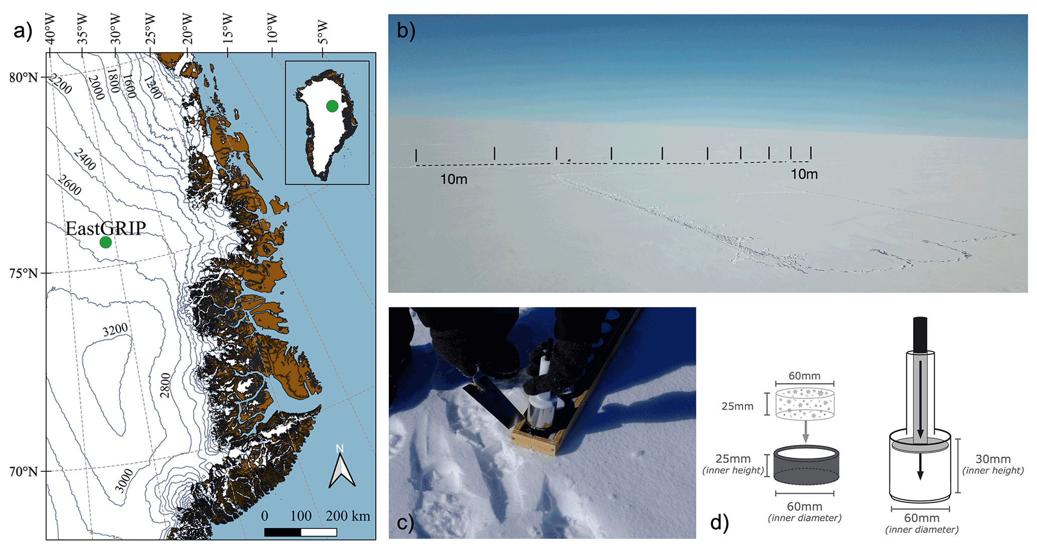
Figure 1(a) A map of Greenland with a green dot indicating the EastGRIP site (Wahl et al., 2021). (b) A photograph of the clean snow area at the field site (Credit: Bruce Vaughn), black lines indicate the SSA sampling transect with 10 m spacing shown as dashed lines. (c) A photograph of SSA sampling cups (Credit: Sonja Wahl), and (d) an illustration of the sampling device from Klein (2014).
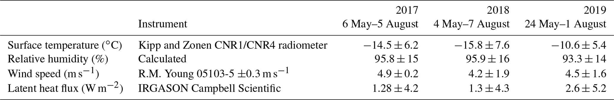
Meteorological data used for this study are from the Program for Monitoring of the Greenland Ice Sheet (PROMICE) Automatic Weather Station set up by the Geological Survey of Denmark and Greenland (GEUS) at EastGRIP in 2016 (Fausto et al., 2021). The data are 10 min mean values for a number of variables. In addition to the surface variables, snow temperature was measured using a thermistor string at 0.1 m intervals during 2017 and 2018 but was modified to 1 m intervals in 2019. An additional thermistor string was thus installed in May 2019, from which we use the 0.1 m measurements. Relevant weather variables for this study are surface temperature (calculated from longwave radiation down and longwave radiation up with longwave emissivity set at 0.97), air temperature and wind speed (Van As, 2011). Mean weather conditions vary between sampling years, as outlined in Table 1, with prevailing westerly winds throughout the sampling seasons.
An eddy covariance (EC) measurement tower was set up at EastGRIP for every summer observation period (Madsen et al., 2019; Wahl et al., 2021). Here we use the 30 min latent heat flux (LE) measurements which are calculated from the measurement of humidity fluxes between the surface and atmosphere. Positive LE indicates upwards energy flux in the form of sublimation in Table 1. Observations of weather conditions such as ground fog, drifting snow and snowfall were documented each day in the EastGRIP field diary.
Table 1Weather statistics for summer field campaigns in 2017, 2018 and 2019. Mean and standard deviation for weather variables during the three sampling seasons. Surface temperature, relative humidity with reference to ice and wind speed use PROMICE weather station based on 10 min measurements. Latent heat flux, a 30 min mean upwards flux from the eddy covariance tower.
2.2 Accumulation, snow sampling and subsequent measurements
Each summer season of 2017, 2018 and 2019, snow samples were taken once a day, primarily in the morning, from May to August at 10 sampling sites. Each site was marked by a stick, along a 90 m transect running perpendicular to the prevailing wind direction (285∘ N (Wahl et al., 2021)) with 10 m spacing upwind of the EastGRIP camp to ensure clean snow (Fig. 1b). The specific dates for each season are given in Table 1. The precise location of each sample was marked by a small stick to ensure the adjacent snow is sampled the next day and to avoid sampling snow from different depths. A 6 cm diameter sampling device (cup) collected the top 2.5 cm of surface snow (Fig. 1c and d). Snow density is determined using the weight of each snow sample with a known volume. Sticks were placed at each sampling site at the start of each season to measure snow height, that is, the distance between the snow surface and top of the stick with a ruler with an uncertainty margin of ±0.5 cm. Accumulation, used here to describe the change in snow height (cm), was calculated using the cumulative sum of the daily difference between measurements of snow height from each site. The resultant datasets consist of daily measurements of four parameters at each of the 10 sampling sites: SSA, density, snow accumulation and stable water isotopes. The field season for 2018 started on 5 May, 9 d earlier than 2017 (14 May), and 22 d earlier than 2019 (27 May). The meteorological data are re-sampled to the SSA sampling time periods.
2.3 SSA measurements
Each snow sample is placed into the Ice Cube sampling container below an infra-red (IR) laser diode (wavelength of 1310 nm), where the SSA is calculated based on IR hemispherical reflectance, as explained in Gallet et al. (2009). More information on the Ice Cube device can be found in Zuanon (2013). Gallet et al. (2009) show that SSA measurements for snow with density of 200 kg m−3 and SSA of 35 m2 kg−1 mostly reflect the top 1 cm of a 2.5 cm snow sample when using 1310 nm radiation, due to the e-folding depth. The properties of each 2.5 cm snow sample will determine the e-folding depth (i.e. the depth to which the light irradiances within the snowpack is reduced to (approximately 37 %) of its initial value), with higher SSA and density causing a decreased e-folding depth. Given that the mean snow density from all field seasons is 293 kg m−3 (307 ± 40, 278 ± 47, 294 ± 50 kg m−3 for 2017, 2018 and 2019 respectively) and the mean SSA is 37.5 m2 kg−1, the measurement of the SSA values will be weighted towards the top <1 cm of the 2.5 cm sample. However, recent studies have shown that the SSA values obtained from the instrument used here (Ice Cube) agree well with measurements from computed microtomography on the same samples (Martin and Schneebeli, 2022). Further, our data are in fairly good agreement with remote sensing products (Kokhanovsky et al., 2019; Vandecrux et al., 2022). Thus we consider our SSA values as representative for the upper 2.5 cm surface snow.
The light reflected from the snow samples is converted into inter-hemispheric IR reflectance using a calibration curve based on methane absorption methods (Gallet et al., 2009). A radiative-transfer model is used to retrieve SSA from inter-hemispherical IR reflectance. To avoid influence from solar radiation, SSA was measured inside a white tent or in a snow cave kept at temperatures between −5 and −20 ∘C. We assume an uncertainty of 10 % for SSA measurements between 5 and 130 m2 kg−1 (Gallet et al., 2009).
2.4 Surface snow isotopes
Individual SSA samples were put in separate bags and subsequently measured for water isotopic composition. Thus, every day the 10 SSA samples have a corresponding isotopic composition. The resultant isotope value is the average composition over the top 2.5 cm of snow. Each sample was kept frozen during transportation and storage. The samples were then analysed at Alfred Wegener Institute in Bremerhaven using cavity ring-down spectroscopy instruments (Picarro L-2120-i and L-2140-i) following the protocol of Van Geldern and Barth (2012). This technique produces δ18O and δD measurements with an estimated uncertainty of 0.15 ‰ and 0.8 ‰ respectively. The values calculated for d-excess have an estimated uncertainty of 1 ‰.
2.5 Data analysis
2.5.1 Defining SSA decay events
Freshly deposited snow has a high SSA that slowly decreases through time due to snow metamorphism. Based on this understanding, two terms are defined:
-
SSA increase: Increases in SSA indicate deposition events in the form of precipitation or deposited snowdrift.
-
SSA decrease: Decreases in SSA are due to snow metamorphism and other post-depositional processes such as wind scouring and, in a few cases, surface hoar formation, where the SSA decreases.
SSA decays are primarily identified in the time series to quantify snow metamorphism and corresponding isotopic change during precipitation-free periods. Surface conditions are considered to remove events with surface snow layer perturbations via deposition or erosion by the wind.
A threshold is derived to systematically identify periods of rapid SSA decay – hereafter referred to as “SSA decay events”. SSA decay events captured by this threshold are defined by the peak SSA value (Day-0), through to the next increase in SSA. A set of criteria are applied to the SSA decay events to avoid events with wind-perturbed surfaces. While in Antarctica, drifting of unconsolidated snow has been observed at mean hourly wind speeds as low as 4.5 m s−1 at 2 m height above the surface (Birnbaum et al., 2010), a study from northeast Greenland, with similar conditions to EastGRIP, documented snowdrift starting at 6 m s−1 (Christiansen, 2001), due to warmer temperatures facilitating bonding of the surface snow (Li and Pomeroy, 1997). Additional field-diary observations from EastGRIP document significant snowdrift when wind speeds exceed 7 m s−1. Based on these observations, two wind speed categories are defined.
-
Low-wind events: The first includes events with daily maximum wind speed (computed from 10 min averaged wind speed) consistently below 6 m s−1, hereafter referred to as “low-wind events”, where negligible surface perturbation is ensured.
-
Moderate-wind events: A second category considers events with daily maximum wind speed between 6 and 7 m s−1, hereafter “moderate-wind events”. The inclusion of these events facilitates an assessment of the influence of wind speed on SSA decay.
Subsequent isotopic analysis is first broadly applied to both low- and moderate-wind events over 1 and 2 d periods, followed by a focused assessment of isotopic change, and corresponding temperature flux is applied to low-wind events alone given the assurance of unperturbed snow. All events with wind speed above 7 m s−1 are excluded from analysis.
2.5.2 Modelling surface snow metamorphism
The first empirical SSA decay model, Eq. (1), was proposed by Cabanes et al. (2003), who described a temperature-dependent exponential decay based on snow samples collected from the Alps (Cabanes et al., 2003) and the Canadian Arctic (Cabanes et al., 2002). Legagneux et al. (2003) found Eq. (2) to best describe experimental SSA decay under controlled laboratory conditions.
In both Eqs. (1) and (2), SSA(t) is the SSA value at a time, t, in days since the initial SSA value, SSA0, and α is the decay rate. Parameters A and B in Eq. (2) were found to be arbitrarily related to the decay rate and initial SSA of each sample. To improve the physical basis of the model, the theory of Ostwald ripening, describing grain growth driven by thermodynamic instability, was implemented into the model (Legagneux et al., 2004). Equation (3) has two parameters, τ and n; τ is the decay rate and n relates to theoretical grain growth. The physical model was further developed by Flanner and Zender (2006) to incorporate a physical quantification of the parameters including information about temperature, temperature gradient, and density. Based on these three conditions, they created a look-up table for τ and n.
Taillandier et al. (2007) proposed two equations based on Eq. (2) to define the decay rate under isothermal and temperature gradient conditions where they were able to directly incorporate a mean surface temperature parameter (Tm). Here we use the model for temperature gradient conditions (Eq. 9 in Taillandier et al., 2007).
Building upon these previous studies, we define an empirical SSA decay model using continuous daily SSA measurements from EastGRIP to describe the behaviour of surface snow SSA in polar summer conditions (Cabanes et al., 2002, 2003; Flanner and Zender, 2006; Legagneux et al., 2002, 2003; Taillandier et al., 2007). A recent study at EastGRIP has shown the significant heterogeneity in surface snow due to post-depositional reworking from the wind (Zuhr et al., 2021), and therefore each sample location is treated individually to avoid the smoothing out of localised signals when averaging.
3.1 EastGRIP meteorological conditions
Meteorological variables over the three sampling seasons vary substantially, as shown in Fig. 2. Air temperatures were below −30 ∘C between 5–8 May in 2018. Such low temperatures were not recorded for 2017 and 2019. Moreover, when comparing the period from 27 May with 5 August of each year (duration of 2019 season), 2018 air temperatures (−13.3 ∘C) were still 0.5 ∘C lower than 2017 and 3.2 ∘C lower than 2019 (Table 1).
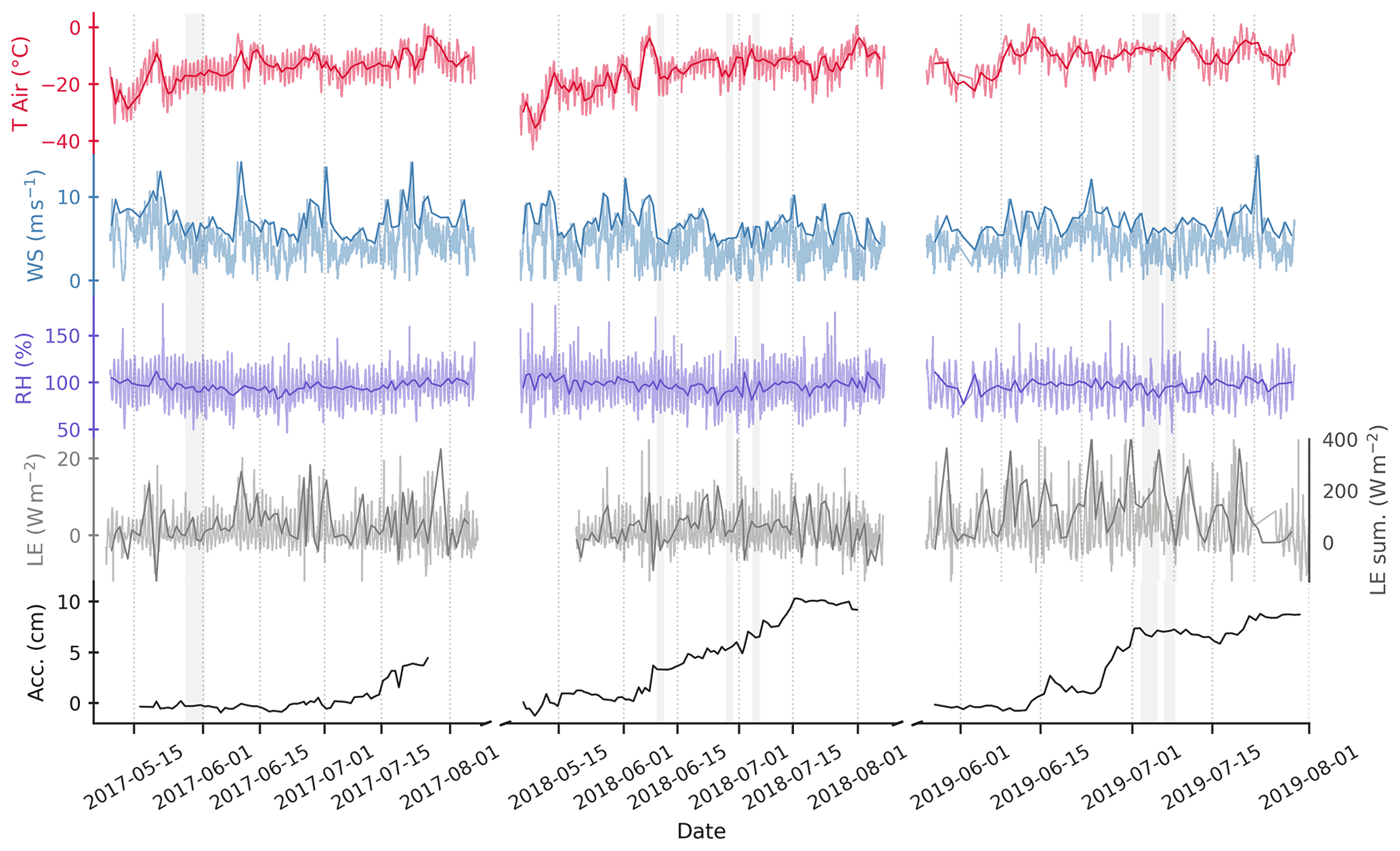
Figure 2Time series of the ambient conditions during the sampling periods. Data cover the specific sampling periods each year. The 10 min mean data from the AWS are presented for air temperature, wind speed and relative humidity. Mean values (bold lines) are shown for air temperature and relative humidity, while daily maximum is shown for wind speed. Latent heat flux data are 30 min averages from the eddy covariance tower, with the daily sum shown in bold. Snow accumulation is presented in the lower panel as the daily mean over the 10 sampling sites (see Sect. 2.2). Grey bars indicate the derived SSA decay events.
The 2017 season was characterised by high wind intrusions of >13 m s−1 at approximately 20 d intervals. Considering all three sampling years, the average daily maximum wind speed is 7 m s−1, with 209 out of the total 237 sampling days having maximum wind speed above 5 m s−1. The distributions of daily maximum wind speed compared to 10 min mean values are found in the Appendix Fig. A1. Net accumulation was observed during all seasons, with 4.8, 9.3 and 8.6 cm accumulated for the 2017, 2018 and 2019 field seasons respectively. In addition, the total sum of LE during 2019 was 30 % greater than in 2018 indicating strong sublimation. Eddy covariance LE measurements are supported by LE from AWS observations which indicate the same magnitude of difference between the years.
3.1.1 Spatial and temporal snow surface variability
Spatial and temporal variability – defined as the daily standard deviation over transect and the standard deviation of the daily mean values over the season respectively – is observed in SSA, δ18O and d-excess throughout the field seasons of 2017, 2018 and 2019 (Fig. 3), with highest spatial variability in isotopic composition. SSA is characterised by peaks, often corresponding to high spatial variability, followed by gradual decreases over a number of days, the SSA decay feature which is most prominent during 2017 and corresponds to negligible or decreasing accumulation. High SSA values at the start of the 2018 season (daily mean 88 m2 kg−1) correspond to low and spatially homogeneous δ18O.
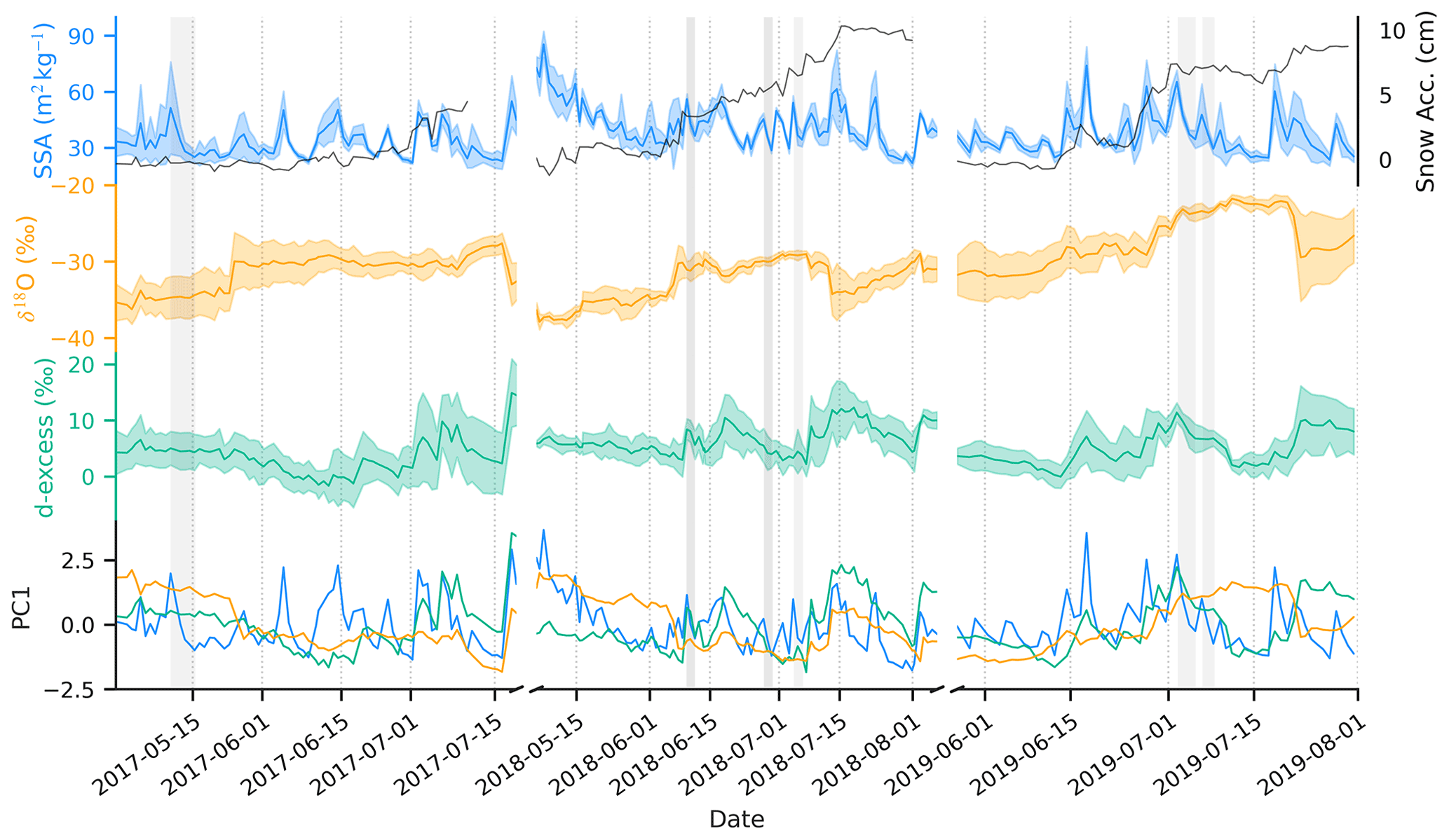
Figure 3Time series of SSA (blue), δ18O (orange), d-excess (green) and the first principal components (PC1) of each variable in the lower panel. Bands in the upper three panels show spatial standard deviation between the 10 sampling sites. The secondary y axis in the top panel shows the average snow accumulation. The grey bars indicate the SSA decay events.
Inter-annual difference is observed in δ18O, with seasonal mean values of −31.6 ± 2.1 ‰, −32.7 ± 1.3 ‰ and −27.3 ± 2.1 ‰ for 2017, 2018 and 2019 respectively (Fig. 3). Throughout the season δ18O follows a gradual increasing trend from May to August concurrent with increasing temperatures. Cases of abrupt decreases (−10 ‰) are observed in the late summer, for example, on 12 July in 2018 and 25 July in 2019, originating from late-summer snowfall events. Note that the 2019 field season started approximately 15 d later than 2017 and 2018, resulting in a bias towards mid-summer conditions. No clear seasonal trend is observed in d-excess, but rather there are periods of gradual decrease in d-excess during periods with no accumulation in all years. The most apparent is from 15 May to 14 June in 2017 corresponding to 0 cm net-accumulation (Fig. 3). The maximum daily spread in δ18O and d-excess is approximately 15 ‰, indicating strong surface heterogeneity.
Empirical orthogonal function (EOF) analysis is applied to the data to identify the dominant modes of variance in both the temporal and spatial dimensions for each parameter – SSA, δ18O and d-excess. Using a confidence interval of 95 % (p<0.05), the relationship between SSA and isotopic composition is tested for all 10 identical samples, covering the entire measurement period. The spatial and temporal principal components returned for each variable by the EOF are presented in Fig. 3. During 2017, 2018 and 2019 all variables have one dominant mode of variance, or principal component (PC1). PC1 of SSA (PC1SSA) explains 61 %, 77 % and 72 % of the variance for the respective years, PC1 of δ18O (PC1) explains 69 %, 83 % and 75 % of the total variance respectively, while PC1 of d-excess (PC1dxs) explains 47 %, 51 % and 60 %.
Results from the EOF analysis reveal distinct differences between the sampling years, most prevalent is the opposing regime from 2018 to 2019. During 2018, PC1 and PC1dxs have an inverse correlation in the spatial dimension (), and a significant positive correlation between PC1 and PC1dssa in the temporal dimension (p<0.05, r=0.5) (Figs. A2 and A3). By contrast, data from 2019 are characterised by significant positive correlations between PC1SSA and PC1dxs in both the spatial (p<0.05, r=0.75) and temporal dimensions (p>0.05, r=0.3), while no relationship is observed between PC1 and PC1dxs. During 2017, there is a weak positive correlation for the temporal component of PC1SSA and PC1dxs (p<0.05, r=0.3), and the temporal PC1 and PC1dxs (p<0.05, r=0.4). There is an apparent shift after 15 July where PC1dxs transitions from co-varying with PC1 to co-varying with PC1SSA. Figures A2 and A3 in the Appendix illustrate the spatial and temporal components of the EOF results.
3.2 SSA decay events
3.2.1 Observations
In agreement with Eq. (1), we observe a relationship between the initial SSA and the subsequent magnitude of decrease when evaluating the SSA decay events (Fig. 3). From the years 2017, 2018 and 2019 a total of 21 events are identified that fulfil the SSA decay criteria (as defined in Sect. 2.5.1). These events are named E1, E2 etc. (Table A1). Using the thresholds defined in Sect. 2.5.1, 15 out of the 21 events are excluded from the analysis due to risk of surface perturbations. Of the six events, two are in the low-wind category (E10 and E11), and four in the moderate-wind category (E1, E13, E18 and E19). Both E10 and E11 had consistent clear sky conditions. Note that E11 was preceded by ground fog, and not snowfall (Table A1).
The rate of SSA decay is strongly influenced by the initial SSA during the decay period (Fig. 4), showing that the rate of change is proportional to the absolute value, as described by an exponential decay law ( and for low- and moderate-wind events respectively). The mean air temperature for all SSA decay events was between −17.3 and −7 ∘C. The first day of each event is characterised by the largest change in SSA, followed by a decrease in magnitude over the subsequent days, with negligible change in SSA below 22 m2 kg−1.
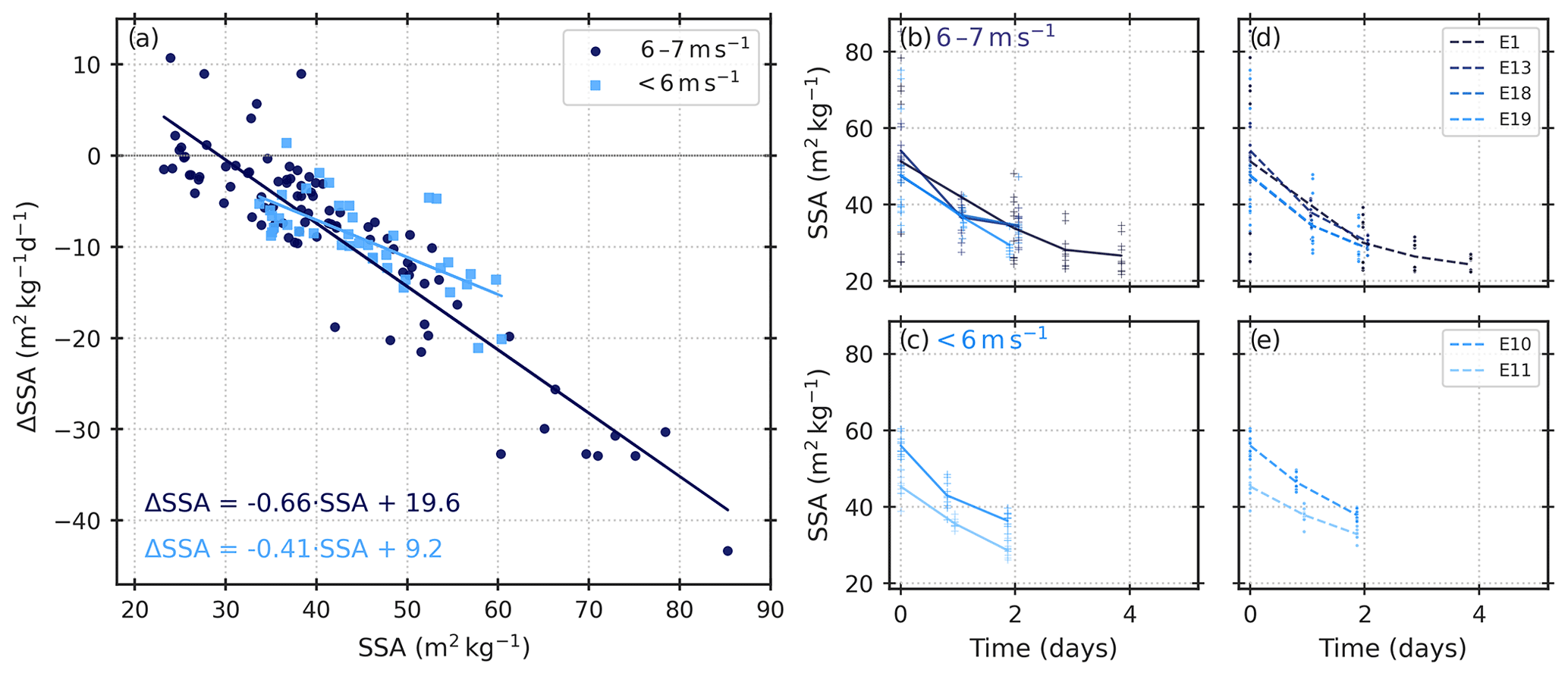
Figure 4Linear regressions for change in SSA against the SSA for the low-wind (light blue) and moderate-wind (dark blue) SSA decay events (a) considering all individual samples. The observed SSA decays are shown for the moderate-wind events (b), and the low-wind events (c), followed by the modelled SSA decays for the respective events in (d) and (e). The legend in (d) and (e) corresponds to the SSA decay event number in Table A1.
3.2.2 Model
The SSA decay rate is quantified by plotting the rate of change in SSA per day against the absolute SSA value for all 10 sampling sites for low- (E10 and E11) and moderate-wind (E1, E13, E18 and E19) events (Fig. 4a). We observe a linear relationship between the change in SSA from one day to the next (ΔSSA) and SSA.
The SSA decay model for EastGRIP is constructed using the differential equation for the linear relationship between ΔSSA and absolute SSA. Solving the differential equation with respect to time (t) produces the SSA decay model defined as Eq. (5), which follows the equation structure of Eq. (1):
where SSA(t) is the SSA measurement at a given time in days since the first measurement (initial SSA), SSA0 is the initial SSA value, and α is the decay rate. An offset of 22 m2 kg−1 is required to account for the non-zero asymptote, and is defined as the SSA value where the derivative of SSA is equal to 0 m2 kg−1. The decay rate, determined by the slope of the linear regressions in Fig. 4, is higher for moderate-wind SSA decay events (−0.66 m2 kg−1 d−1) than for low-wind SSA decay events (−0.41 m2 kg−1 d−1). Within the temperature range of low- and moderate-wind SSA decay events from this study, there is no observable temperature dependence of the SSA decay rate. However, such a temperature dependence is clear in events which were excluded due to potential surface perturbations, where there is a decrease in decay rate and an increase in the background SSA value with low temperatures (Fig. A4). Our results indicate a slower rate of decay under decreased wind speed conditions.
3.2.3 Model performance comparison
Model performance is tested by comparing daily predicted decrease with the 10 daily observations, and by comparing model predictions from this study with those from Flanner and Zender (2006), hereafter referred to as “FZ06”, and the model defined by Taillandier et al. (2007), hereafter “T07”, as defined in Sect. 2.5.2. Residuals between our model and the observations are normally distributed, suggesting no systematic errors in model predictions. The RMSE between our model predictions and observed SSA is 2.48 and 2.60 m2 kg−1 for the low-wind and moderate-wind SSA decay events respectively.
Table 2RMSE values for model evaluation. Model predictions are compared with observations for both the daily mean SSA values (Mean) and the 10 individual SSA measurements (Individual). For the low-wind events, α in Eq. (5) is −0.41 m2 kg−1 d−1. For moderate-wind events α in Eq. (5) is −0.66 m2 kg−1 d−1. FZ06 parameters τ and n are defined from the look-up table in Flanner and Zender (2006). T07 uses the mean surface temperature for each event as an input parameter.
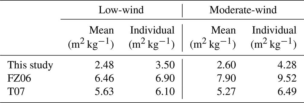
Parameter values for τ and n in FZ06 are defined for each event based on mean density, surface temperature and temperature gradient using the extensive look-up table referenced in Flanner and Zender (2006). FZ06 consistently overestimates the SSA decay rate, with residuals increasing throughout the events (Fig. A5). T07 generally underestimates the SSA decay rate of low- and moderate-wind events, with the largest errors associated with E1, the event featuring the lowest temperatures and highest wind speeds. RMSE values presented in Table 2 show that the model from this study predicts the observed SSA decay with the least error.
3.3 Isotopic change during SSA decay events
3.3.1 Low- and moderate-wind event analysis
The following sections assess the snow isotopic change during the low- and moderate-wind events. For both low- and moderate-wind events, the change in d-excess is plotted against the change in SSA (Fig. 5), after the first and second day of each event. Here, we include the analysis of the change in d-excess after the second day (referred to as “a 2 d change”), presented in Table 3 for each low- and moderate-wind event.
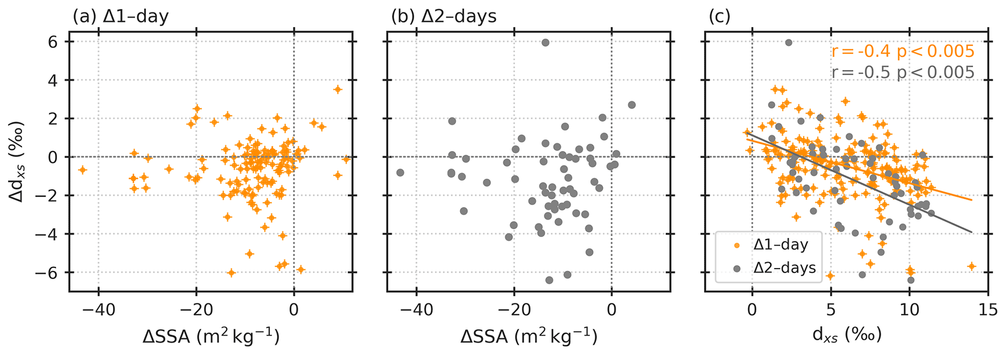
Figure 5Isotopic changes during all of the analysed events are shown, with each point indicating a specific sampling site. The daily change in d-excess (dxs) and SSA is presented in (a), change in d-excess and SSA over the first 2 d of each event is shown in (b), and the respective changes in d-excess are plotted against the absolute d-excess values in (c). Linear regressions are included for daily change (orange) and 2 d change (grey).
Table 3Table of isotopic change for decay events. Mean values on Day-0 and Day-2 of each event, and percentage change over this 2 d period are presented for δ18O, d-excess and SSA. Low-wind events (bold text) and moderate-wind events are presented.
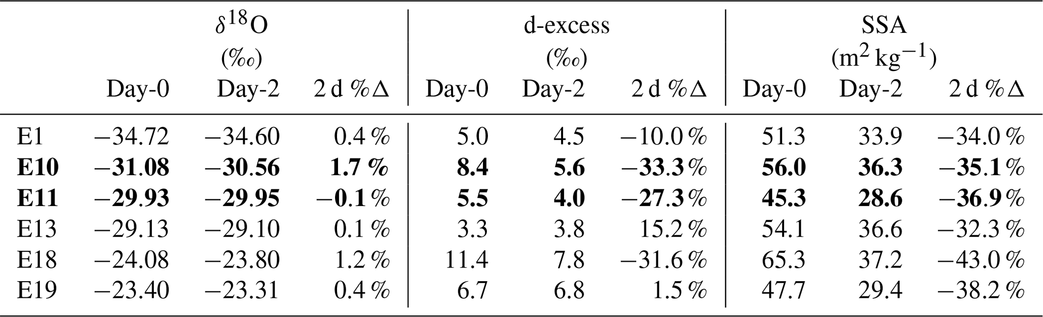
Both δ18O and d-excess change from the initial value (Day-0) in all events, with the percentage change in d-excess being the same order of magnitude as for SSA, and an order of magnitude higher than that of δ18O. Three out of six events are characterised by increasing δ18O and decreasing d-excess after 2 d. E1, E13 and E19 deviate from this pattern. E13 and E19 both correspond to total increase in δ18O and d-excess, whereas E11 is characterised by a slight decrease in δ18O and decrease in d-excess (Table 3). The Δd-excess over a 1 d period indicates a slight negative skew around a mean of −0.3 ‰. Four of six events (61 % of all sample sites) experience a decrease in d-excess by Day-2. The mean is shifted to −1.2 ‰ over a 2 d period with decreases in d-excess documented in 45 out of the 60 samples (75 %) during precipitation-free periods with minimal surface perturbation. Initial d-excess is observed to have a significant influence on the magnitude of d-excess decrease over the defined period (Fig. 5c), with high initial d-excess corresponding to the largest decreases in d-excess.
3.3.2 Low-wind event analysis
The following section focuses on latent heat flux (LE) and near-surface temperature gradients (TG) corresponding to isotopic change during low-wind events only. This is to ensure that the surface layer we are analysing is constant throughout the event to avoid inaccurate interpretation of isotopic change. As mentioned in Sect. 3.2, ground fog preceded the SSA peak in E11, concurrent with negligible accumulation recorded. By contrast, the day prior to E10 corresponds to the observation of snowfall (Table A1). Figure 6 shows the relationship between the daily change in isotopic composition for E10 and E11 (Δd-excess and Δδ18O) and SSA (ΔSSA). During E10, significant inverse correlations are observed between Δδ18O and Δd-excess, and between ΔSSA and Δd-excess (, ), while Δδ18O and ΔSSA are positively correlated (r=0.6). By contrast, no significant relationship is observed between the Δ-parameters during E11, where there is negligible change in surface snow δ18O (<0.7 ‰).
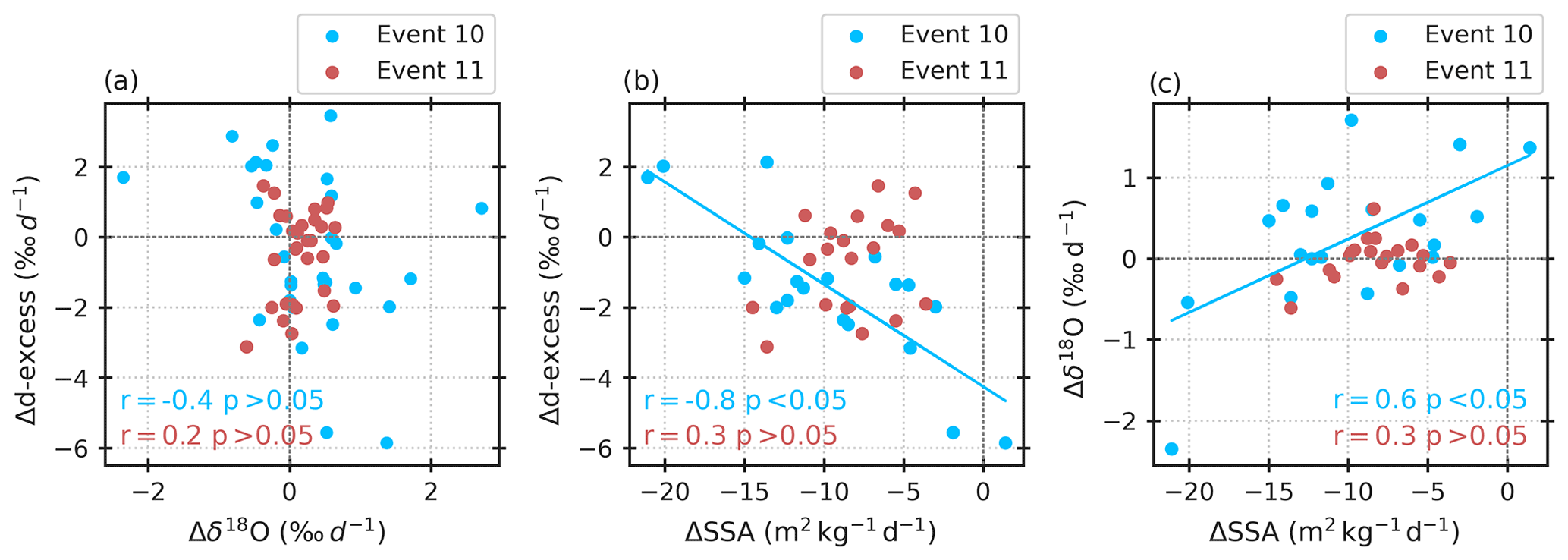
Figure 6Isotopic change analysis for low-wind events, E10 and E11. Panel (a) shows daily change in d-excess against change in δ18O for E10 and E11, (b) shows change in d-excess against change in SSA, and (c) shows change in δ18O and change in SSA. The r and p values for each regression are indicated in the corresponding colours. Only significant linear regressions are indicated with a line.
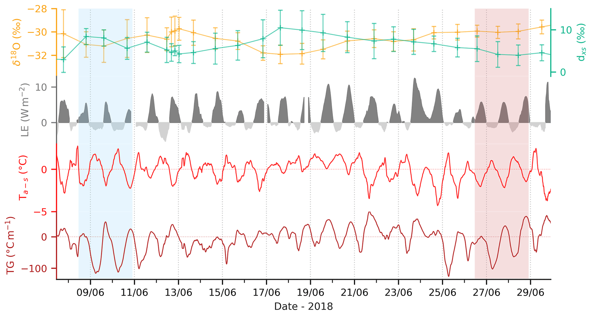
Figure 7LE and temperature gradients for low-wind events. Latent heat flux (LE) (grey), air-surface temperature gradient (TG) (bright red) and surface-10 cm subsurface TG (dark red) during June 2018. E10 (blue) and E11 (red) are highlighted. Dark grey shading in LE indicates sublimation and light grey shows deposition.
The direction of vapour fluxes is inferred using temperature gradients determined from air, surface and subsurface (10 cm depth) temperature data, and LE, measured as an upwards flux. Net sublimation is observed during both E10 and E11, with a total sum of 33.9 and 55.8 W m−2 for the respective events. LE is inversely related to the TG between the air and the surface, with strong sublimation (>10 W m−2), corresponding to a negative TG of 2.5 ∘C between the air and surface on 10 June 2018 (E10). A concurrent upwards vapour flux is observed between the subsurface and surface, most apparent on 11 June 2018 (Day-2 of E10). Negative LEs up to −4 W m−1 are documented each night corresponding to the transition from a negative to positive TG between the air and surface. Net-deposition was recorded between sampling on 9 June at 15:30 UTC and 10 June 10:30 UTC 2018 (first day of E10) corresponding to a decrease in δ18O and d-excess. The subsequent day, characterised by net sublimation, had a large increase in δ18O and a larger decrease in d-excess. Contrary to E10, E11 is characterised by a large decrease in d-excess and a small decrease in δ18O, both concurrent with net-sublimation and strong negative surface-subsurface TG. The air-surface TG during E11 has a lower mean and reduced diurnal amplitude than E10 facilitating sublimation for a longer period.
The new SSA and snow isotopic composition datasets presented in this study have revealed concurrent decreases in d-excess (and δ18O to a lesser degree) and SSA during precipitation-free periods with minimal snow drift. A simple empirical model describing the SSA decay rate under different wind regimes reveals more rapid SSA decay when wind speeds are higher. The following sections look first at why existing models tend to be inaccurate when predicting in situ SSA decay at the surface, followed by a second section discussing the possible mechanisms driving the relationship between SSA and d-excess during precipitation-free periods.
4.1 SSA decay at EastGRIP
Events of rapid SSA decay at EastGRIP are best described by an exponential decay function, in agreement with observations from Cabanes et al. (2003). No cold events ( ∘C) are captured within the event criteria, potentially indicating that warmer temperatures are needed to induce such change in SSA over the time period, or that the local synopticity favours precipitation (bringing snow with high SSA) coincident with low temperature and high winds during the summer. Events captured by the threshold with mean temperatures below −20 ∘C are likely capturing wind erosion that exposes sub-surface snow with low SSA. The narrow temperature range of SSA decay events does not facilitate a conclusive definition of a temperature-dependent decay rate (Cabanes et al., 2003; Legagneux et al., 2003; Flanner and Zender, 2006; Taillandier et al., 2007). We instead assess the influence of wind speed on the SSA decay rate and observe a more rapid SSA decay with increased wind speed, which can be explained by increased ventilation of saturated pore air acting as a catalyst for snow metamorphism (Cabanes et al., 2003; Flanner and Zender, 2006; Neumann and Waddington, 2004). While wind erosion cannot be definitively ruled out even after applying the criteria described in Sect. 2.5.1, high wind speeds are documented to increase SSA via the re-deposition of fragmentation and sublimated snow crystals after suspension (Domine et al., 2009), meaning that SSA changes of this nature would not be captured in our analysis.
Unsurprisingly, given the parameters are fit to the data, the model defined in this study predicts observed SSA decay for the low- and moderate-wind events with the lowest RMSE. T07 (Eq. 4) underestimated the observed SSA decay rate in all the low- and moderate-wind events, except for E18. The largest error is associated with E1, which also had the highest mean wind-speed (6.9 m s−1) of all analysed events. The tendency for T07 to underestimate the observed SSA decay can be explained by the additional influence of wind speed which accelerates SSA decay (Cabanes et al., 2002) but is not considered in either T07 or FZ06. By contrast, FZ06 consistently overestimates the observed SSA decay rate, most pronounced in E10 and E18. The original parameter values τ and n of FZ06 were tuned to data from alpine regions, potentially explaining the poor fit.
The simple empirical model presented here is limited to conditions at EastGRIP within a narrow temperature range (−18 to −7 ∘C) and therefore might be unsuitable for sites with different conditions. However, large errors when using the models from the literature indicate that the low-latitude tuning and exclusion of wind effects are not optimal for predicting surface snow SSA decay at EastGRIP. Our study is limited by a relatively small number of unperturbed SSA decay events, hampering statistical evaluation over longer timescales.
4.2 Isotopic change during SSA decay events
4.2.1 Low-wind events
In the absence of snowfall or other surface perturbations, multi-day periods of snow metamorphism correspond to change in snow isotopic composition. We observe decreasing d-excess with SSA through time suggesting that the mechanisms driving snow metamorphism also influence the isotopic composition. However, the mechanisms linking these changes are unclear and are not always consistent in space and time. The following section explores the possible mechanisms driving isotopic change during SSA decay events, by assessing the LE and TG conditions during events with minimal surface perturbations.
Two key mechanisms are expected to drive the rapid SSA decay and concurrent change in snow isotopic composition: (1) snow grain growth via diffusion of interstitial water vapour due to near-surface temperature gradients (Colbeck, 1983; Ebner et al., 2017; Touzeau et al., 2018), observed to cause a decrease in d-excess and slight increase in δ18O in the defined snow layer (Colbeck, 1983; Ebner et al., 2017; Touzeau et al., 2016); (2) grain rounding via sublimation from convex regions of snow grains (Neumann and Waddington, 2004), causing an increase in δ18O and a significant decrease in d-excess of the remaining snow (Ritter et al., 2016; Madsen et al., 2019; Casado et al., 2021; Hughes et al., 2021; Wahl et al., 2021). Sublimation is enhanced by ventilation of the saturated pore air, known as “wind-pumping” (Neumann and Waddington, 2004). We note that isothermal metamorphism driven by Ostwald ripening also causes a decrease in SSA (Ebner et al., 2015), but is associated with minimal change in bulk isotopic composition which was not observed in our analysis. However, conditions that favour Ostwald ripening were not observed in our analysis.
Increases in δ18O and decreases in d-excess during E10 can be attributed to a combination of (1) and (2) based on the observation of net-sublimation and high amplitude diurnal TG variability over the course of the event. Net-deposition was measured during the period between 9 June at 15:30 UTC and 10 June 10:30 UTC 2018, corresponding to an overall decrease in δ18O, agreeing with previous studies (Stenni et al., 2016; Casado et al., 2021; Feher et al., 2021), and a minimal decrease in d-excess, which is not necessarily expected during deposition. However, disequilibrium between water vapour isotopic composition and snow isotopic composition may explain the deviation from expectation (Wahl et al., 2022). Although ground fog was documented on the day preceding E11, no significant deposition is observed in the LE data in the day preceding E11, indicating the absence of lasting surface hoar formation. The 30 % decrease in d-excess concurrent with no change in δ18O suggests strong kinetic fractionation during E11. Continuous variations in δ18O and d-excess throughout June 2018 (Fig. 7) show no clear relationship to total LE or temperature gradients. Field experiments looking at sub-diurnal variability show a stronger dependence of snow isotopic composition on LE (Hughes et al., 2021), potentially explaining the lack of a strong diurnal relationship.
Conclusively identifying these mechanisms requires measurements of water vapour isotopes to model the fractionation effects. In the absence of these data, we infer potential explanations for isotopic change during the low-wind events. Our analysis suggests that SSA of the surface snow is strongly influenced by surface-subsurface TG and wind speed, while the changes in isotopic composition are likely to be influenced by other factors, such as the magnitude of vapour–snow isotopic disequilibrium during sublimation (Wahl et al., 2022). Decoupling the influence of sublimation and interstitial diffusion within the snow requires additional measurements of isotopic composition of atmospheric water vapour to model associated fractionation effects (Wahl et al., 2022). Our results show that while snow isotopic composition does indeed change during SSA decay events, predicting the magnitude, and even the sign, of the isotopic change associated with snow metamorphism is not possible when information about the interstitial vapour isotopic composition is missing.
4.2.2 Inter-annual variability
The recurring difference in snow characteristics and temperature conditions during 2019 compared to 2017 and 2018 could be explained by the shifting phase of the North Atlantic Oscillation (NAO), which is in positive phase during 2017 and 2018 (below-average temperatures) and in negative phase during 2019. A similar pattern is observed in the snow isotopes when considering the period between 27 May and 1 August where the mean δ18O value during 2019 was −27.3 ‰, which is 4.3 ‰ higher than 2018 (−31.6 ‰) and 3.6 ‰ higher than 2017 (−30.9 ‰). While the difference in mean δ18O can plausibly be explained by a 3.2 ∘C mean air temperature difference, the isotope-SSA covariance is not so straightforward.
The positive mode of PC1SSA (Fig. 3) can be interpreted as increases in SSA from depositional events, such as precipitation, and wind-fragmented snowdrift (Domine et al., 2009), while the negative mode is associated with snow metamorphism or wind erosion (Cabanes et al., 2002, 2003; Legagneux et al., 2003, 2004; Taillandier et al., 2007; Flanner and Zender, 2006). Based on this interpretation, a covariance between PC1SSA and PC1dxs or PC1 indicates that the mechanisms controlling SSA variability also influence the isotopic composition. We observe a decoupling of the temporal variance in d-excess from that of δ18O (Fig. 3) in 2019. This difference may be related to the recorded transition from winter to summer in 2017 and 2018, but not in 2019.
Ongoing work to disentangle the processes driving change in isotopic composition – sublimation from surface or interstitial vapour diffusion between layers in the pore space – is vital for precise climate reconstruction in ice cores (Touzeau et al., 2018; Casado et al., 2021; Hughes et al., 2021; Wahl et al., 2021). Future studies would benefit from obtaining direct measurements of the isotopic composition of precipitation and surface hoar, to determine the fraction of such deposits in the SSA samples. Furthermore, a quantitative representation of vapour fluxes in the surface snow rather than the temperature-gradient-based approximation used in this study would provide a basis from which to quantify the relative influence of fractionation during sublimation and interstitial diffusion.
4.3 Implications and perspectives
Documented changes in snow isotopic composition during surface snow metamorphism have potential implications for interpretation of stable water isotope records from ice cores, given that the current interpretation assumes the precipitation signal is preserved (Dansgaard, 1964). Variations of d-excess in ice core records are attributed to changes in source region, source region conditions and kinetic fractionation occurring during snow crystal formation in supersaturated clouds (Stenni et al., 2010; Jouzel and Merlivat, 1984). However, we show that there are substantial changes in d-excess during precipitation-free periods supporting recent work showing that post-depositional factors add complexity to the traditional interpretation of ice core water isotope records. Greenland ice core records show abrupt decreases in d-excess corresponding to warming transitions, which is attributed to change in moisture source regions (Steffensen et al., 2008). Results presented in our study document decreases in snow d-excess during surface snow metamorphism associated with temperature gradients and sublimation, potentially contributing to the low d-excess values during warm periods.
The findings of this exploratory study reiterate the importance of quantifying the isotopic fractionation effects associated with processes driving snow metamorphism during precipitation-free periods. Moreover, the inter-annual variability observed at EastGRIP between 2018 and 2019 suggests that precipitation intermittency, temperature (gradients) and wind regimes play a role in isotopic change, which is not readily identified in the surface snow SSA data.
This study addresses the rapid SSA decay driven by surface snow metamorphism. In particular, the study aims to explore how rapid SSA decay relates to changes in isotopic composition of the surface snow in the dry accumulation zone of the Greenland Ice Sheet. Ten individual snow samples were collected daily over a 90 m transect at EastGRIP in the period between May and August of 2017, 2018 and 2019. SSA and isotopic composition were measured for each sample. Periods of snow metamorphism after deposition events were defined using SSA measurements to extract periods of rapid decreases in SSA. An exponential SSA decay model () was constructed to describe empirically surface snow metamorphism in summer conditions for polar snow, with surface temperatures above -20 ∘C and with minimal surface perturbation. Two event categories were defined based on wind speed, with an upper threshold of 7 m s−1 to minimise chance of snowdrift. Higher wind speeds increase the SSA decay rate due to enhanced snow metamorphism with increased ventilation of the pore space.
Changes in isotopic composition corresponding to post-depositional processes driving SSA decay are observed in all low- and moderate-wind events. A decrease in d-excess from Day-0 to Day-2 is observed in four out of the six events with no precipitation. Further analysis of low-wind SSA decay events indicates that the combined effects of vapour diffusion and diurnal LE variability causes isotopic fractionation of the surface snow in the absence of precipitation. The differing fractionation effects are expected to be the result of vapour–snow isotopic disequilibrium. A strong correlation observed between SSA and d-excess found in 2019 was not present for 2018. We suggest that this is due to strong sublimation corresponding to high temperatures during 2019.
In summary, our results support documentation of fractionation during sublimation and deposition between the snow surface and atmosphere, indicating that the precipitation isotopic composition signal is not always preserved during the processes driving surface snow metamorphism. Observations of post-depositional decrease in d-excess during rapid SSA decay hints at local processes influencing the d-excess signal, and therefore an interpretation as source region signal alone is insufficient.
Table A1Description of conditions for SSA decays captured by decreased threshold. Duration and conditions for all 21 events defined by the threshold. Observations were made of snowfall, snowdrift and ground fog. Presented here are the dates, event number, mean surface temperature (ST), maximum wind speed (WS), accumulation (A), and surface conditions including those recorded during the day (24 h) preceding each event (Day-1), cloud cover, observations of surface perturbations during the events based on field observations (Day-0–n), and finally the wind speed category for SSA decay event analysis (Event category). In the “Surface conditions” columns, S, SD and F stand for snowfall, snowdrift and ground fog respectively. C in “Cloud cover” indicates clear sky and O indicates overcast.
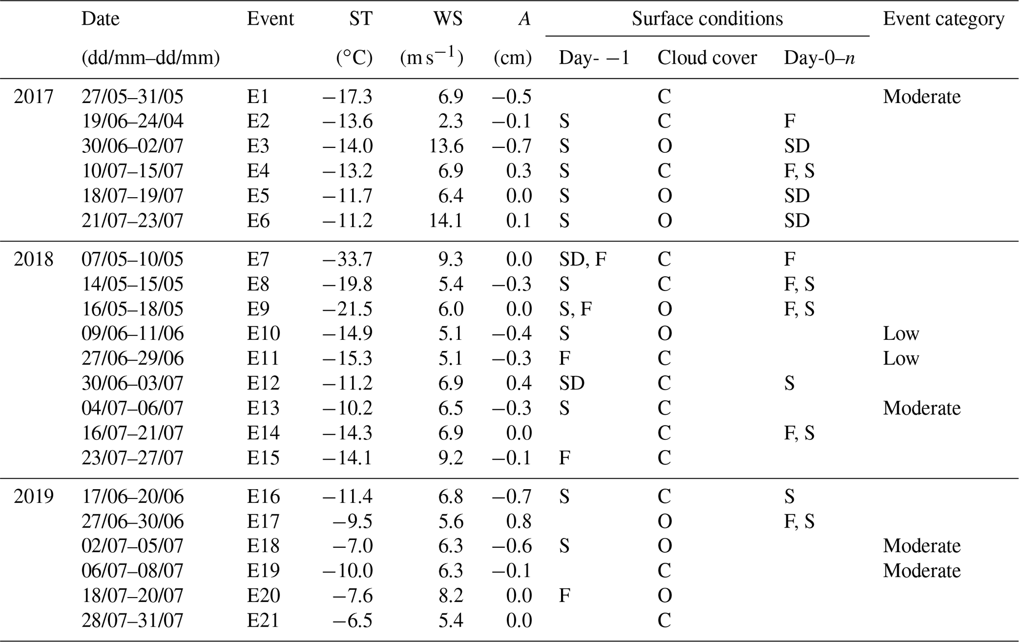

Figure A1Histograms showing (a) the daily maximum values and (b) the 10 min mean values for all sampling days of 2017, 2018 and 2019. The black line indicates the mean.
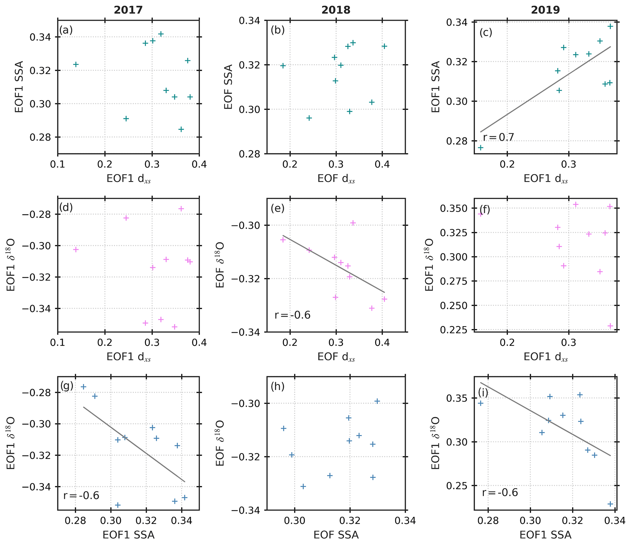
Figure A2Results from the EOF analysis showing the relationship between SSA, d-excess and δ18O in the spatial dimension. Linear regressions are included in plots with significant correlations (p<0.05) between variables.
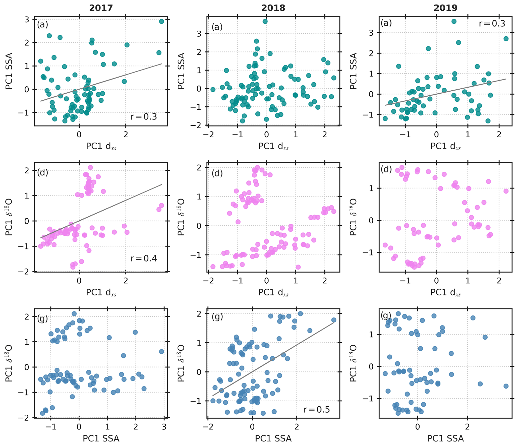
Figure A3Results from the EOF analysis showing the relationship between SSA, d-excess and δ18O in the temporal dimension. Linear regressions are included in plots with significant correlations (p<0.05) between variables.
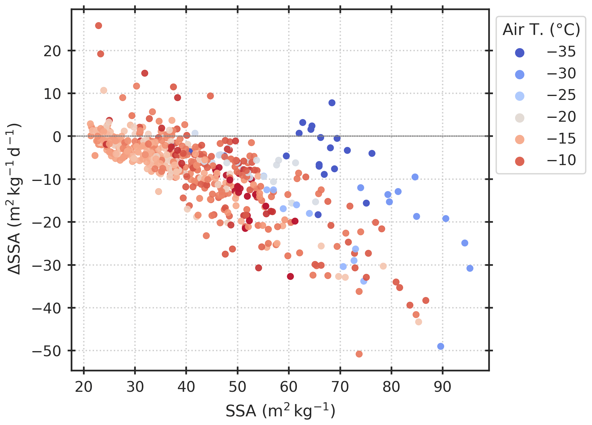
Figure A4The change in SSA after 1 d (Day-1 to Day-0) plotted against the absolute value from Day-0 for all 21 SSA decay events (E1–E21 in Table A1) captured by the decrease threshold described in Sect. 2.5.1. The markers are coloured by mean air temperature between samplings (i.e. the mean air temperature from the time between sampling on Day-0 and Day-1).
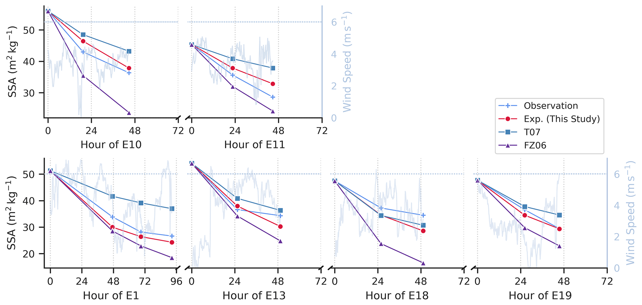
Figure A5SSA decay model evaluation and a comparison with observations. Included models are the decay model from this study and the existing decay models from Flanner and Zender (2006), FZ06, and Taillandier et al. (2007), T07. The 10 min averaged wind speed is shown on the secondary y axis, with the 6 m2 kg−1 thresholds indicated. Low-wind events E10 and E11 are shown in the upper panel, and moderate-wind events are shown in the lower panel (E1, E13, E18 and E19).
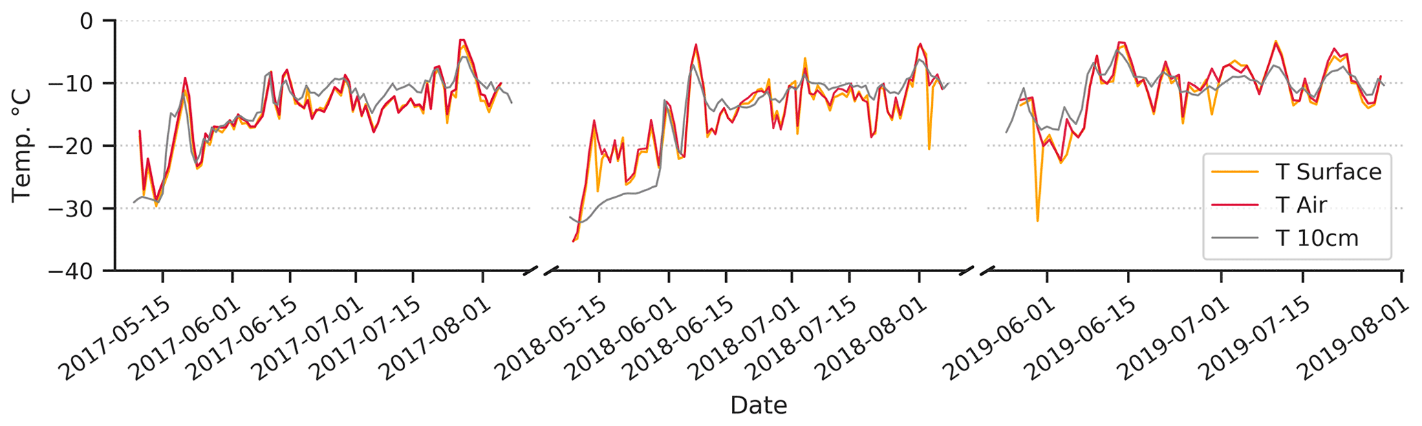
Figure A6Daily mean 2 m air temperature (red), surface temperature (yellow) and 10 cm subsurface temperature (grey). The data are presented for the 2017, 2018 and 2019 measurement campaigns.
The SSA, density and accumulation data for all sampling years is available on the PANGAEA database with the DOI: https://doi.org/10.1594/PANGAEA.946763 (Steen-Larsen et al., 2022). Snow isotope data is available at DOI: https://doi.pangaea.de/10.1594/PANGAEA.946729 (Hörhold et al., 2022). Data from the Programme for Monitoring of the Greenland Ice Sheet (PROMICE) 400 were provided by the Geological Survey of Denmark and Greenland (GEUS) at http://www.promice.dk (last access: 1 October 2021, Fausto et al., 2021). Eddy Covariance Tower measurement are available on the PANGAEA database with the DOI: https://doi.org/10.1594/PANGAEA.928827 (Steen-Larsen and Wahl, 2021).
HCSL, AKF and RHS designed the study together. AKF, SW, MH, MB, AZ, SK and HCSL carried out the data collection and measurements. RHS, AKF and HCSL worked directly with the data. RHS, AKF, KV and HCSL prepared the manuscript with contributions from all co-authors. AKF contributed largely to the manuscript text and structure. HCSL designed and administrated the SNOWISO project.
The contact author has declared that none of the authors has any competing interests.
Publisher’s note: Copernicus Publications remains neutral with regard to jurisdictional claims in published maps and institutional affiliations.
This project has received funding from the European Research Council (ERC) under the European Union’s Horizon 2020 research and innovation program: Starting Grant-SNOWISO (grant agreement 759526). EastGRIP is directed and organised by the Centre for Ice and Climate at the Niels Bohr Institute, University of Copenhagen. It is supported by funding agencies and institutions in Denmark (A. P. Møller Foundation, University of Copenhagen), USA (US National Science Foundation, Office of Polar Programs), Germany (Alfred Wegener Institute, Helmholtz Centre for Polar and Marine Research), Japan (National Institute of Polar Research and Arctic Challenge for Sustainability), Norway (University of Bergen and Bergen Research Foundation), Switzerland (Swiss National Science Foundation), France (French Polar Institute Paul-Emile Victor, Institute for Geosciences and Environmental research), and China (Chinese Academy of Sciences and Beijing Normal University).
This research has been supported by the H2020 European Research Council (SNOWISO (grant no. 759526)).
This paper was edited by Melody Sandells and reviewed by Florent Dominé and Dorothea Elisabeth Moser.
Birnbaum, G., Freitag, J., Brauner, R., König, G., König-Langlo, K., Schulz, E., Kipfstuhl, S., Oerter, H., Reijmer, C. H., Schlosser, E., Faria, S. H., Ries, H., Loose, B., Herber, A., Duda, M. G., Powers, J. G., Manning, K. W., and Van Den Broeke, M. R.: Strong-wind events and their influence on the formation of snow dunes: observations from Kohnen station, Dronning Maud Land, Antarctica, J. Glaciol., 56, 891–902, 2010. a
Cabanes, A., Legagneux, L., and Dominé, F.: Evolution of the specific surface area and of crystal morphology of Arctic fresh snow during the ALERT 2000 campaign, Atmos. Environ., 36, 2767–2777, https://doi.org/10.1016/S1352-2310(02)00111-5, 2002. a, b, c, d, e, f, g
Cabanes, A., Legagneux, L., and Dominé, F.: Rate of evolution of the specific surface area of surface snow layers, Environ. Sci. Technol., 37, 661–666, https://doi.org/10.1021/es025880r, 2003. a, b, c, d, e, f, g, h, i, j, k
Carmagnola, C. M., Domine, F., Dumont, M., Wright, P., Strellis, B., Bergin, M., Dibb, J., Picard, G., Libois, Q., Arnaud, L., and Morin, S.: Snow spectral albedo at Summit, Greenland: measurements and numerical simulations based on physical and chemical properties of the snowpack, The Cryosphere, 7, 1139–1160, https://doi.org/10.5194/tc-7-1139-2013, 2013. a, b
Casado, M., Landais, A., Picard, G., Münch, T., Laepple, T., Stenni, B., Dreossi, G., Ekaykin, A., Arnaud, L., Genthon, C., Touzeau, A., Masson-Delmotte, V., and Jouzel, J.: Archival processes of the water stable isotope signal in East Antarctic ice cores, The Cryosphere, 12, 1745–1766, https://doi.org/10.5194/tc-12-1745-2018, 2018. a
Casado, M., Münch, T., and Laepple, T.: Climatic information archived in ice cores: impact of intermittency and diffusion on the recorded isotopic signal in Antarctica, Clim. Past, 16, 1581–1598, https://doi.org/10.5194/cp-16-1581-2020, 2020. a
Casado, M., Landais, A., Picard, G., Arnaud, L., Dreossi, G., Stenni, B., and Prié, F.: Water Isotopic Signature of Surface Snow Metamorphism in Antarctica, Geophys. Res. Lett., 48, e2021GL093382, https://doi.org/10.1029/2021GL093382, 2021. a, b, c, d, e, f, g
Christiansen, H. H.: Snow-cover depth, distribution and duration data from northeast Greenland obtained by continuous automatic digital photography, Ann. Glaciol., 32, 102–108, 2001. a
Ciais, P. and Jouzel, J.: Deuterium and oxygen 18 in precipitation: Isotopic model, including mixed cloud processes, J. Geophys. Res., 99, 793–809, https://doi.org/10.1029/94JD00412, 1994. a
Colbeck, S. C.: Thermodynamics of snow metamorphism due to variations in curvature, J. Glaciol., 26, 291–301, 1980. a
Colbeck, S. C.: Theory of metamorphism of dry snow., J. Geophys. Res., 88, 5475–5482, https://doi.org/10.1029/JC088iC09p05475, 1983. a, b, c
Dansgaard, W.: Stable isotopes in precipitation, Tellus, 16, 436–468, https://doi.org/10.3402/tellusa.v16i4.8993, 1964. a, b, c
Domine, F., Taillandier, A. S., and Simpson, W. R.: A parameterization of the specific surface area of seasonal snow for field use and for models of snowpack evolution, J. Geophys. Res.-Earth, 112, F02031, https://doi.org/10.1029/2006JF000512, 2007. a
Domine, F., Taillandier, A.-S., Cabanes, A., Douglas, T. A., and Sturm, M.: Three examples where the specific surface area of snow increased over time, The Cryosphere, 3, 31–39, https://doi.org/10.5194/tc-3-31-2009, 2009. a, b
Ebner, P. P., Schneebeli, M., and Steinfeld, A.: Tomography-based monitoring of isothermal snow metamorphism under advective conditions, The Cryosphere, 9, 1363–1371, https://doi.org/10.5194/tc-9-1363-2015, 2015. a
Ebner, P. P., Steen-Larsen, H. C., Stenni, B., Schneebeli, M., and Steinfeld, A.: Experimental observation of transient δ18O interaction between snow and advective airflow under various temperature gradient conditions, The Cryosphere, 11, 1733–1743, https://doi.org/10.5194/tc-11-1733-2017, 2017. a, b, c, d
Faber, A.-K., Møllesøe Vinther, B., Sjolte, J., and Anker Pedersen, R.: How does sea ice influence δ18O of Arctic precipitation?, Atmos. Chem. Phys., 17, 5865–5876, https://doi.org/10.5194/acp-17-5865-2017, 2017. a
Fausto, R. S., van As, D., Mankoff, K. D., Vandecrux, B., Citterio, M., Ahlstrøm, A. P., Andersen, S. B., Colgan, W., Karlsson, N. B., Kjeldsen, K. K., Korsgaard, N. J., Larsen, S. H., Nielsen, S., Pedersen, A. Ø., Shields, C. L., Solgaard, A. M., and Box, J. E.: Programme for Monitoring of the Greenland Ice Sheet (PROMICE) automatic weather station data, Earth Syst. Sci. Data, 13, 3819–3845, https://doi.org/10.5194/essd-13-3819-2021, 2021. a, b
Feher, R., Voiculescu, M., Chiroiu, P., and Perşoiu, A.: The stable isotope composition of hoarfrost, Isot. Environ. Health S., 57, 386–399, https://doi.org/10.1080/10256016.2021.1917567, 2021. a
Flanner, M. G. and Zender, C. S.: Linking snowpack microphysics and albedo evolution, J. Geophys. Res.-Atmos., 111, D12208, https://doi.org/10.1029/2005JD006834, 2006. a, b, c, d, e, f, g, h, i, j, k
Flin, F. and Brzoska, J. B.: The temperature-gradient metamorphism of snow: Vapour diffusion model and application to tomographic images, Ann. Glaciol., 49, 17–21, https://doi.org/10.3189/172756408787814834, 2008. a
Gallet, J.-C., Domine, F., Zender, C. S., and Picard, G.: Measurement of the specific surface area of snow using infrared reflectance in an integrating sphere at 1310 and 1550 nm, The Cryosphere, 3, 167–182, https://doi.org/10.5194/tc-3-167-2009, 2009. a, b, c, d, e
Gallet, J.-C., Domine, F., Arnaud, L., Picard, G., and Savarino, J.: Vertical profile of the specific surface area and density of the snow at Dome C and on a transect to Dumont D'Urville, Antarctica – albedo calculations and comparison to remote sensing products, The Cryosphere, 5, 631–649, https://doi.org/10.5194/tc-5-631-2011, 2011. a
Gallet, J.-C., Domine, F., Savarino, J., Dumont, M., and Brun, E.: The growth of sublimation crystals and surface hoar on the Antarctic plateau, The Cryosphere, 8, 1205–1215, https://doi.org/10.5194/tc-8-1205-2014, 2014. a
Genthon, C., Piard, L., Vignon, E., Madeleine, J.-B., Casado, M., and Gallée, H.: Atmospheric moisture supersaturation in the near-surface atmosphere at Dome C, Antarctic Plateau, Atmos. Chem. Phys., 17, 691–704, https://doi.org/10.5194/acp-17-691-2017, 2017. a
Holme, C., Gkinis, V., and Vinther, B. M.: Molecular diffusion of stable water isotopes in polar firn as a proxy for past temperatures, Geochim. Cosmochim. Ac., 225, 128–145, https://doi.org/10.1016/j.gca.2018.01.015, 2018. a
Hörhold, M., Behrens, M., Steen-Larsen, H. C., Faber, A.-K., Kipfstuhl, S., Madsen, M., Meyer, H., Vladimirova, D., Wahl, S., Zuhr, A., Stuart, R. H.: 10 daily measurements of water isotopic composition of the surface 2.5 cm of snow from EastGRIP during summer of 2017–2019, PANGAEA [data set], https://doi.pangaea.de/10.1594/PANGAEA.946729 (last access: 27 February 2023), 2022. a
Hughes, A. G., Wahl, S., Jones, T. R., Zuhr, A., Hörhold, M., White, J. W. C., and Steen-Larsen, H. C.: The role of sublimation as a driver of climate signals in the water isotope content of surface snow: laboratory and field experimental results, The Cryosphere, 15, 4949–4974, https://doi.org/10.5194/tc-15-4949-2021, 2021. a, b, c, d, e, f, g
Johnsen, S. J., Clausen, H. B., Cuffey, K. M., Hoffmann, G., Schwander, J., and Creyts, T.: Diffusion of stable isotopes in polar firn and ice: the isotope effect in firn diffusion, in: Physics of Ice Core Records, Hokkaido University Press, 121–142, http://hdl.handle.net/2115/32465 (last access: 1 October 2021), 2000. a
Johnsen, S. J., Dansgaard, W., and White, J. W.: The origin of Arctic precipitation under present and glacial conditions, Tellus B, 41, 452–468, https://doi.org/10.3402/tellusb.v41i4.15100, 1989. a
Jouzel, J. and Merlivat, L.: Deuterium and oxygen 18 in precipitation: modeling of the isotopic effects during snow formation, J. Geophys. Res., 89, 749–757, https://doi.org/10.1029/jd089id07p11749, 1984. a
Klein, K.: Variability in dry Antarctic firn – Investigations on spatially distributed snow and firn samples from Dronning Maud Land, Antarctica, PhD thesis, University of Bremen, https://doi.org/10013/epic.44893, 2014. a
Kokhanovsky, A., Lamare, M., Danne, O., Brockmann, C., Dumont, M., Picard, G., Arnaud, L., Favier, V., Jourdain, B., Meur, E. L., Di Mauro, B., Aoki, T., Niwano, M., Rozanov, V., Korkin, S., Kipfstuhl, S., Freitag, J., Hoerhold, M., Zuhr, A., Vladimirova, D., Faber, A. K., Steen-Larsen, H. C., Wahl, S., Andersen, J. K., Vandecrux, B., van As, D., Mankoff, K. D., Kern, M., Zege, E., and Box, J. E.: Retrieval of snow properties from the Sentinel-3 Ocean and Land Colour Instrument, Remote Sensing, 11, 2280, https://doi.org/10.3390/rs11192280, 2019. a
Laepple, T., Münch, T., Casado, M., Hoerhold, M., Landais, A., and Kipfstuhl, S.: On the similarity and apparent cycles of isotopic variations in East Antarctic snow pits, The Cryosphere, 12, 169–187, https://doi.org/10.5194/tc-12-169-2018, 2018. a
Landais, A., Barnola, J. M., Kawamura, K., Caillon, N., Delmotte, M., Van Ommen, T., Dreyfus, G., Jouzel, J., Masson-Delmotte, V., Minster, B., Freitag, J., Leuenberger, M., Schwander, J., Huber, C., Etheridge, D., and Morgan, V.: Firn-air δ15N in modern polar sites and glacial-interglacial ice: A model-data mismatch during glacial periods in Antarctica?, Quaternary Sci. Rev., 25, 49–62, https://doi.org/10.1016/j.quascirev.2005.06.007, 2006. a
Legagneux, L. and Domine, F.: A mean field model of the decrease of the specific surface area of dry snow during isothermal metamorphism, J. Geophys. Res.-Earth, 110, F04011, https://doi.org/10.1029/2004JF000181, 2005. a
Legagneux, L., Cabanes, A., and Dominé, F.: Measurement of the specific surface area of 176 snow samples using methane adsorption at 77 K, J. Geophys. Res.-Atmos., 107, 4335–4350, https://doi.org/10.1029/2001JD001016, 2002. a, b
Legagneux, L., Lauzier, T., Dominé, F., Kuhs, W. F., Heinrichs, T., and Techmer, K.: Rate of decay of specific surface area of snow during isothermal experiments and morphological changes studied by scanning electron microscopy, Can. J. Phys., 81, 459–468, https://doi.org/10.1139/p03-025, 2003. a, b, c, d, e
Legagneux, L., Taillandier, A. S., and Domine, F.: Grain growth theories and the isothermal evolution of the specific surface area of snow, J. Appl. Phys., 95, 6175–6184, https://doi.org/10.1063/1.1710718, 2004. a, b, c, d, e, f
Li, L. and Pomeroy, J. W.: Estimates of threshold wind speeds for snow transport using meteorological data, J. Appl. Meteorol., 36, 205–213, https://doi.org/10.1175/1520-0450(1997)036<0205:EOTWSF>2.0.CO;2, 1997. a
Linow, S., Hörhold, M. W., and Freitag, J.: Grain-size evolution of polar firn: A new empirical grain growth parameterization based on X-ray microcomputer tomography measurements, J. Glaciol., 58, 1245–1252, https://doi.org/10.3189/2012JoG11J256, 2012. a, b
Madsen, M. V., Steen-Larsen, H. C., Hörhold, M., Box, J., Berben, S. M., Capron, E., Faber, A. K., Hubbard, A., Jensen, M. F., Jones, T. R., Kipfstuhl, S., Koldtoft, I., Pillar, H. R., Vaughn, B. H., Vladimirova, D., and Dahl-Jensen, D.: Evidence of Isotopic Fractionation During Vapor Exchange Between the Atmosphere and the Snow Surface in Greenland, J. Geophys. Res.-Atmos., 124, 2932–2945, https://doi.org/10.1029/2018JD029619, 2019. a, b, c
Martin, J. and Schneebeli, M.: Impact of the sampling procedure on the specific surface area of snow measurements with the IceCube, EGUsphere [preprint], https://doi.org/10.5194/egusphere-2022-501, 2022. a
Masson-Delmotte, V., Landais, A., Stievenard, M., Cattani, O., Falourd, S., Jouzel, J., Johnsen, S. J., Dahl-Jensen, D., Sveinsbjornsdottir, A., White, J. W., Popp, T., and Fischer, H.: Holocene climatic changes in Greenland: Different deuterium excess signals at Greenland Ice Core Project (GRIP) and NorthGRIP, J. Geophys. Res.-Atmos., 110, D14102, https://doi.org/10.1029/2004JD005575, 2005. a
Merlivat, L. and Jouzel, J.: Global climatic interpretation of the deuterium-oxygen 16 relationship for precipitation., J. Geophys. Res., 84, 5029–5033, https://doi.org/10.1029/JC084iC08p05029, 1979. a
Neumann, T. A. and Waddington, E. D.: Effects of firn ventilation on isotopic exchange, J. Glaciol., 50, 183–194, 2004. a, b, c
Picard, G., Domine, F., Krinner, G., Arnaud, L., and Lefebvre, E.: Inhibition of the positive snow-albedo feedback by precipitation in interior Antarctica, Nat. Clim. Change, 2, 795–798, https://doi.org/10.1038/nclimate1590, 2012. a
Picard, G., Royer, A., Arnaud, L., and Fily, M.: Influence of meter-scale wind-formed features on the variability of the microwave brightness temperature around Dome C in Antarctica, The Cryosphere, 8, 1105–1119, https://doi.org/10.5194/tc-8-1105-2014, 2014. a
Picard, G., Arnaud, L., Caneill, R., Lefebvre, E., and Lamare, M.: Observation of the process of snow accumulation on the Antarctic Plateau by time lapse laser scanning, The Cryosphere, 13, 1983–1999, https://doi.org/10.5194/tc-13-1983-2019, 2019. a
Pinzer, B. and Schneebeli, M.: Temperature gradient metamorphism is not a classical coarsening process, in: ISSW 09 – International Snow Science Workshop, Proceedings, Davos, Switzerland, 27 September to 2 October 2009, 58–61, 2009. a, b
Pinzer, B. R., Schneebeli, M., and Kaempfer, T. U.: Vapor flux and recrystallization during dry snow metamorphism under a steady temperature gradient as observed by time-lapse micro-tomography, The Cryosphere, 6, 1141–1155, https://doi.org/10.5194/tc-6-1141-2012, 2012. a
Ritter, F., Steen-Larsen, H. C., Werner, M., Masson-Delmotte, V., Orsi, A., Behrens, M., Birnbaum, G., Freitag, J., Risi, C., and Kipfstuhl, S.: Isotopic exchange on the diurnal scale between near-surface snow and lower atmospheric water vapor at Kohnen station, East Antarctica, The Cryosphere, 10, 1647–1663, https://doi.org/10.5194/tc-10-1647-2016, 2016. a, b, c
Schaller, C. F., Freitag, J., and Eisen, O.: Critical porosity of gas enclosure in polar firn independent of climate, Clim. Past, 13, 1685–1693, https://doi.org/10.5194/cp-13-1685-2017, 2017. a
Sime, L. C., Risi, C., Tindall, J. C., Sjolte, J., Wolff, E. W., Masson-delmotte, V., and Capron, E.: Warm climate isotopic simulations : what do we learn about interglacial signals in Greenland ice cores?, Quaternary Sci. Rev., 67, 59–80, https://doi.org/10.1016/j.quascirev.2013.01.009, 2013. a
Sodemann, H., Masson-Delmotte, V., Schwierz, C., Vinther, B. M., and Wernli, H.: Interannual variability of Greenland winter precipitation sources: 2. Effects of North Atlantic Oscillation variability on stable isotopes in precipitation, J. Geophys. Res. Atmos., 113, D12111, https://doi.org/10.1029/2007JD009416, 2008. a
Sokratov, S. A. and Golubev, V. N.: Snow isotopic content change by sublimation, J. Glaciol., 55, 823–828, https://doi.org/10.3189/002214309790152456, 2009. a
Steen-Larsen, H. C. and Wahl, S.: 2 m processed sensible and latent heat flux, friction velocity and stability at EastGRIP site on Greenland Ice Sheet, summer 2019, PANGAEA [data set], https://doi.org/10.1594/PANGAEA.928827, 2021. a
Steen-Larsen, H. C., Sveinbjörnsdottir, A. E., Peters, A. J., Masson-Delmotte, V., Guishard, M. P., Hsiao, G., Jouzel, J., Noone, D., Warren, J. K., and White, J. W. C.: Climatic controls on water vapor deuterium excess in the marine boundary layer of the North Atlantic based on 500 days of in situ, continuous measurements, Atmos. Chem. Phys., 14, 7741–7756, https://doi.org/10.5194/acp-14-7741-2014, 2014. a, b
Steen-Larsen, H. C., Hörhold, M., Kipfstuhl, S., Faber, A.-K., Freitag, J., Hughes, A. G., Madsen, M., Behrens, M. K., Meyer, H., Vladimirova, D., Wahl, S., Zuhr, A., Stuart, R. H.: 10 daily surface measurements over 90 m transect, SSA, Density and Accumulation, from EastGRIP summer (May–August) of 2016–2019, PANGAEA [data set], https://doi.org/10.1594/PANGAEA.946763, 2022. a
Steffensen, J. P., Andersen, K. K., Bigler, M., Clausen, H. B., Dahl-Jensen, D., Fischer, H., Goto-Azuma, K., Hansson, M., Johnsen, S. J., Jouzel, J., Masson-Delmotte, V., Popp, T., Rasmussen, S. O., Röthlisberger, R., Ruth, U., Stauffer, B., Siggaard-Andersen, M. L., Sveinbjörnsdottir, Ø. E., Svensson, A., and White, J. W.: High-resolution greenland ice core data show abrupt climate change happens in few years, Science, 321, 680–684, https://doi.org/10.1126/science.1157707, 2008. a
Stenni, B., Masson-Delmotte, V., Selmo, E., Oerter, H., Meyer, H., Röthlisberger, R., Jouzel, J., Cattani, O., Falourd, S., Fischer, H., Hoffmann, G., Iacumin, P., Johnsen, S. J., Minster, B., and Udisti, R.: The deuterium excess records of EPICA Dome C and Dronning Maud Land ice cores (East Antarctica), Quaternary Sci. Rev., 29, 146–159, https://doi.org/10.1016/j.quascirev.2009.10.009, 2010. a
Stenni, B., Scarchilli, C., Masson-Delmotte, V., Schlosser, E., Ciardini, V., Dreossi, G., Grigioni, P., Bonazza, M., Cagnati, A., Karlicek, D., Risi, C., Udisti, R., and Valt, M.: Three-year monitoring of stable isotopes of precipitation at Concordia Station, East Antarctica, The Cryosphere, 10, 2415–2428, https://doi.org/10.5194/tc-10-2415-2016, 2016. a
Taillandier, A. S., Domine, F., Simpson, W. R., Sturm, M., and Douglas, T. A.: Rate of decrease of the specific surface area of dry snow: Isothermal and temperature gradient conditions, J. Geophys. Res.-Earth, 112, F03003, https://doi.org/10.1029/2006JF000514, 2007. a, b, c, d, e, f, g, h
Touzeau, A., Landais, A., Stenni, B., Uemura, R., Fukui, K., Fujita, S., Guilbaud, S., Ekaykin, A., Casado, M., Barkan, E., Luz, B., Magand, O., Teste, G., Le Meur, E., Baroni, M., Savarino, J., Bourgeois, I., and Risi, C.: Acquisition of isotopic composition for surface snow in East Antarctica and the links to climatic parameters, The Cryosphere, 10, 837–852, https://doi.org/10.5194/tc-10-837-2016, 2016. a
Touzeau, A., Landais, A., Morin, S., Arnaud, L., and Picard, G.: Numerical experiments on vapor diffusion in polar snow and firn and its impact on isotopes using the multi-layer energy balance model Crocus in SURFEX v8.0, Geosci. Model Dev., 11, 2393–2418, https://doi.org/10.5194/gmd-11-2393-2018, 2018. a, b
Van As, D.: Warming, glacier melt and surface energy budget from weather station observations in the Melville Bay region of northwest Greenland, J. Glaciol., 47, 208–220, https://doi.org/10.3189/002214311796405898, 2011. a
Vandecrux, B., Box, J. E., Wehrlé, A., Kokhanovsky, A. A., Picard, G., Niwano, M., Hörhold, M., Faber, A. K., and Steen-Larsen, H. C.: The Determination of the Snow Optical Grain Diameter and Snowmelt Area on the Greenland Ice Sheet Using Spaceborne Optical Observations, Remote Sensing, 14, 932, https://doi.org/10.3390/rs14040932, 2022. a
Van Geldern, R. and Barth, J. A.: Optimization of instrument setup and post-run corrections for oxygen and hydrogen stable isotope measurements of water by isotope ratio infrared spectroscopy (IRIS), Limnol. Oceanogr.-Meth., 10, 1024–1036, https://doi.org/10.4319/lom.2012.10.1024, 2012. a
Vinther, B. M., Buchardt, S., Clausen, H., Dahl-Jensen, D., Johnsen, S., Fisher, D., Koerner, R., Raynaud, D., Lipenkov, V., Andersen, K., Blunier, T., Rasmussen, S., Steffensen, J., and Svensson, A.: Holocene thinning of the Greenland ice sheet, Nature, 461, 385–388, 2009. a
Wahl, S., Steen-Larsen, H. C., and Reuder, J.: Quantifying the Stable Water Isotopologue Exchange between Snow Surface and Lower Atmosphere by Direct Flux Measurements, J. Geophys. Res.-Atmos., 126, e2020JD034400, https://doi.org/10.1029/2020jd034400, 2021. a, b, c, d, e, f, g
Wahl, S., Steen-Larsen, H. C., Hughes, A. G., Dietrich, L. J., Zuhr, A., Behrens, M., Faber, A., and Hörhold, M.: Atmosphere-Snow Exchange Explains Surface Snow Isotope Variability, Geophys. Res. Lett., 49, e2022GL099529, https://doi.org/10.1029/2022GL099529, 2022. a, b, c, d
Zuanon, N.: IceCube, a portable and reliable instrument for snow specific surface area measurement in the field, International Snow Science Workshop, Grenoble – Chamonix Mont-Blanc, 7–11 October 2013, 1020–1023, https://arc.lib.montana.edu/snow-science/item/1905 (last access: 1 October 2021), 2013. a
Zuhr, A. M., Münch, T., Steen-Larsen, H. C., Hörhold, M., and Laepple, T.: Local-scale deposition of surface snow on the Greenland ice sheet, The Cryosphere, 15, 4873–4900, https://doi.org/10.5194/tc-15-4873-2021, 2021. a