the Creative Commons Attribution 4.0 License.
the Creative Commons Attribution 4.0 License.
 | 14 Mar 2022
Arctic sea ice anomalies during the MOSAiC winter 2019/20
Klaus Dethloff
Stefan Hendricks
Younjoo J. Lee
Helge F. Goessling
Thomas Krumpen
Christian Haas
Dörthe Handorf
Robert Ricker
Vladimir Bessonov
John J. Cassano
Jaclyn Clement Kinney
Robert Osinski
Markus Rex
Annette Rinke
Julia Sokolova
Anja Sommerfeld
During the winter of 2019/2020, as the Multidisciplinary drifting Observatory for the Study of Arctic Climate (MOSAiC) project started its work, the Arctic Oscillation (AO) experienced some of its largest shifts, ranging from a highly negative index in November 2019 to an extremely positive index during January–February–March (JFM) 2020. The permanent positive AO phase for the 3 months of JFM 2020 was accompanied by a prevailing positive phase of the Arctic Dipole (AD) pattern. Here we analyze the sea ice thickness (SIT) distribution based on CryoSat-2/SMOS satellite-derived data augmented with results from the hindcast simulation by the fully coupled Regional Arctic System Model (RASM) from November 2019 through March 2020. A notable result of the positive AO phase during JFM 2020 was large SIT anomalies of up to 1.3 m that emerged in the Barents Sea (BS), along the northeastern Canadian coast and in parts of the central Arctic Ocean. These anomalies appear to be driven by nonlinear interactions between thermodynamic and dynamic processes. In particular, in the Barents and Kara seas (BKS), they are a result of enhanced ice growth connected with low-temperature anomalies and the consequence of intensified atmospherically driven sea ice transport and deformations (i.e., ice divergence and shear) in this area. The Davies Strait, the east coast of Greenland and the BS regions are characterized by convergence and divergence changes connected with thinner sea ice at the ice borders along with an enhanced impact of atmospheric wind forcing. Low-pressure anomalies that developed over the eastern Arctic during JFM 2020 increased northerly winds from the cold Arctic Ocean to the BS and accelerated the southward drift of the MOSAiC ice floe. The satellite-derived and simulated sea ice velocity anomalies, which compared well during JFM 2020, indicate a strong acceleration of the Transpolar Drift relative to the mean for the past decade, with intensified speeds of up to 6 km d−1. As a consequence, sea ice transport and deformations driven by atmospheric surface wind forcing accounted for the bulk of the SIT anomalies, especially in January 2020 and February 2020. RASM intra-annual ensemble forecast simulations with 30 ensemble members forced with different atmospheric boundary conditions from 1 November 2019 through 30 April 2020 show a pronounced internal variability in the sea ice volume, driven by thermodynamic ice-growth and ice-melt processes and the impact of dynamic surface winds on sea ice formation and deformation. A comparison of the respective SIT distributions and turbulent heat fluxes during the positive AO phase in JFM 2020 and the negative AO phase in JFM 2010 corroborates the conclusion that winter sea ice conditions in the Arctic Ocean can be significantly altered by AO variability.
- Article
(16074 KB) - Full-text XML
-
Supplement
(3369 KB) - BibTeX
- EndNote


The temporal evolution of the Arctic sea ice thickness distribution is the result of complex and highly variable interactions within the pack ice and its interactions with atmospheric and oceanic processes (e.g., Belter et al., 2021). Since the late 1970s, remotely sensed measurements have provided Arctic-wide information about changes in sea ice cover (https://nsidc.org/cryosphere/seaice/study/remote_sensing.html, last access: 3 April 2020), which has motivated the development of new satellite products (Zwally et al., 2002; Stern and Moritz, 2002; Spreen et al., 2008; Tilling et al., 2018; Neumann et al., 2019) as well as regionally focused coupled Arctic system models and sea ice prediction systems (e.g., Dorn et al., 2007, 2009; Maslowski et al., 2012) to address stakeholders' need for information related to shipping, resource extraction and climate monitoring. Oceanic heat inflows into the Arctic Ocean (through the Bering Strait from the Pacific side and through the Barents Sea (BS) and Fram Strait from the Atlantic side) and sea ice impact the vertical structure of the upper halocline downstream. Schlichtholz (2019) demonstrated that more than 80 % of the variance of the leading variability mode in the winter Arctic sea ice concentration from 1981–2018, with the main centers of action appearing in the BS region, can be explained by the preceding summertime temperature anomalies in Atlantic water inflow from the Norwegian Sea. The variability of Arctic sea ice distribution, its drift and deformation is connected to atmospheric teleconnection patterns and cyclonic systems, which both influence the dynamic ice redistribution and thermodynamic sea ice growth and melt. with impacts on the dynamic ice redistribution and thermodynamic sea ice growth and melt. Wind patterns affect the ice variability of the BS and Barents and Kara seas (BKS) through momentum transfer, advection of cold and dry or warm and humid air, the forcing of warm Atlantic water inflow into the BS, and increased or decreased turbulent surface heat fluxes.
Since the BS is a shallow marginal sea, the wind-driven circulation together with tidal mixing effectively move the bulk of the heat in the Atlantic water to the atmosphere, and only a small amount of this heat enters the deep Arctic Basin (Gammelsrød et al., 2009; Onarheim et al. 2015). Therefore, oceanic heat convergence and atmospheric winds appear to be the main drivers of the evolution of BS ice cover. Northerly winds influence sea ice advection mainly in winter during strong wind events, and processes related to large-scale atmospheric circulation patterns, cyclonic activity, the length of the freezing season and the remaining sea ice volume after the summer melt season are of also of importance to sea ice variability in winter.
The observed decline in Arctic sea ice was identified as a main contributor to changes in the large-scale Arctic Oscillation (AO) pattern and mid-latitude climate changes during winter; see, e.g., Cohen et al. (2014). The origin of AO changes between positive and negative phases has been attributed to declining sea ice in Arctic regions (Screen et al., 2013), planetary–synoptic circulation adjustment processes (Dethloff et al., 2006; Sokolova et al., 2007), changes in Siberian snow cover (Cohen et al., 2012), weakening and warming of the stratospheric polar vortex (Kim et al., 2014), natural variability (McCusker et al., 2016) and anthropogenic greenhouse gases (Johannessen et al., 2004). As pointed out by Ding et al. (2019), Arctic sea ice changes nonuniformly under the influence of multiple internal or external factors.
The BS has been considered a key region for the observed fast changes in the Arctic climate due to the intense air–sea interaction (as pointed out by Smedsrud et al., 2013) and anomalous turbulent heat fluxes that impact the AO winter phase via mediation of surface heat fluxes at the ocean–atmosphere interface (Liptak and Strong, 2014). An inflow of warm Atlantic water influences the sea ice cover in the BS, and its decline there has been connected to a northward shift of the Gulf Stream front (Sato et al., 2014). So far, despite many modeling efforts, no consensus has been reached with regard to the connection of Arctic sea ice reductions to AO phase changes, with some studies pointing to positive AO changes (e.g., Orsolini et al., 2013) while others suggest negative changes (Peings and Magnusdottir, 2014). Nakamura et al. (2015) showed that a stationary Rossby wave response to sea ice reduction in the BS might introduce an anomalous circulation pattern similar to the negative AO phase and tropospheric cyclonic anomalies over Siberia formed by the Rossby wave response to a wave source in the BKS region. Nie et al. (2019) emphasized the role of initial stratospheric conditions and wind anomalies in November. Westerly wind anomalies result in positive AO winter phases, and the reverse happens for easterly initial anomalies. Kolstad and Screen (2019) showed that the correlation between autumn BKS ice and the winter North Atlantic Oscillation is nonstationary and contains considerable decadal variability. They argued that the recently observed high correlation can be explained purely by internal variability, a view supported by Blackport et al. (2019). Gong et al. (2020) emphasized an Arctic wave train propagating from the subtropics through the mid-latitudes into the Arctic and back into the mid-latitudes, which is recharged and amplified in the Arctic through anomalous surface heat flux anomalies over the Greenland Sea and the BKS. The processes responsible for the observed sea ice loss in the Arctic are influenced by coupled nonlinear atmosphere–ocean–sea ice feedbacks in different regions of the Arctic Ocean basin, as discussed by Bushuk et al. (2019). The two-way interaction between the ocean, sea ice and atmosphere impacts (via surface turbulent heat fluxes) the lower troposphere, which feeds back with changed thermodynamic ice growth conditions and atmospheric wind stress forcing. Zhao et al. (2019) described positive and negative feedbacks related to the AO, as revealed by surface heat fluxes in the Nordic seas based on NCEP reanalysis data.
Platov et al. (2020) noted three modes of surface wind forcing on the Arctic sea ice. The first, the oceanic mode, is associated with cyclonic or anticyclonic circulation in the Arctic Ocean, as discussed by Proshutinsky and Johnson (1997). The second, the dipole mode, accelerates or slows down the Transpolar Drift. The third, the Atlantic mode, weakens or intensifies the cyclonic gyre in the northern North Atlantic, corresponding to the atlantification trend (Barton et al., 2018) in the BKS. Wang et al. (2021) studied the impact of atmospheric wind forcing on Arctic sea ice characteristics through simulations with a coupled ocean–sea ice model and identified spatial sea ice patterns connected with AO, Arctic Dipole (AD) and Beaufort High modes.
Trofimov et al. (2020) describe a temperature decrease of more than 1 ∘C for Atlantic water flowing into the BS since 2015 and argue that lower temperatures, in combination with a reduced inflow during winter, caused the increases in BS winter sea ice observed in recent years. The sea surface temperature averaged over the southern BS dropped significantly in 2019, and its annual mean value was the lowest since 2011. In the Eurasian Basin of the Arctic Ocean, Polyakov et al. (2020) noticed a weakening of the ocean stratification over the halocline, which isolates intermediate-depth Atlantic water from the surface mixed layer. The oceanic turbulent heat fluxes increased and were greater than 10 W m−2 for the winters of 2016–2018, with significant impacts on the sea ice loss in this region. These oceanic changes have the potential to increase baroclinic instability in the early Arctic winter troposphere, which impacts on synoptic-scale structures in autumn and planetary waves in late winter (Jaiser et al., 2012), increases Arctic storm activity, and plays an important role in meridional heat transport into the BKS (Long and Perrie, 2017).
The connection between sea ice and atmospheric circulation is critical to understanding the abrupt circulation changes experienced by the atmosphere and sea ice during winter 2019/20. The leading atmospheric variability pattern moved from a below-average negative AO phase in November 2019 to a highly positive and persistent AO phase during January–March 2020. The positive AO phase in the Arctic troposphere was accompanied by cold surface temperatures and enhanced near-surface wind anomalies, and was connected with an exceptionally strong and persistent cold stratospheric polar vortex (Lawrence et al., 2020). During the MOSAiC winter of 2019/20, the tropospheric wave activity and wave forcing was weak and the stratospheric vortex developed an unusual configuration that reflected planetary waves back into the troposphere and impacted the lower atmospheric circulation. The distribution and transport of Arctic sea ice is driven by near-surface wind fields that are dominated in winter by the Beaufort High, which yields an anticyclonic sea ice drift within the Beaufourt Gyre. Its northern branch, the Transpolar Drift, moves sea ice from the Siberian coast across the deep basin toward the Fram Strait and the Nordic seas. The positive (negative) AO is characterized by low (high) sea-level pressure anomalies over the Arctic that lead to cyclonic (anticyclonic) atmospheric circulation anomalies (Armitage et al., 2018), a contracted (expanded) Beaufort Gyre circulation (Kwok et al., 2013) and respective shifts of the Transpolar Drift. Proshutinsky and Johnson (1997) discussed the alternating appearance of cyclonic and anticyclonic circulation regimes of the wind-driven Arctic Ocean. During cyclonic regimes, low sea-level atmospheric pressure dominated over the Arctic Ocean, driving sea ice and the upper ocean counterclockwise, whereas during anticyclonic circulation regimes, high sea-level pressure dominated, leading to clockwise circulation. Circulation structures connected to the AD pattern have been discussed by Watanabe et al. (2006), Vihma et al. (2012) and Lei et al. (2019) in relation to its role in exporting sea ice from the Arctic.
During winter 2019/20, the international research project MOSAiC (Multidisciplinary drifting Observatory for the Study of Arctic Climate) used the research icebreaker RV Polarstern (Polarstern: Alfred-Wegener-Institut Helmholtz-Zentrum für Polar- und Meeresforschung, 2017), operated by the German Alfred Wegener Institute, Helmholtz Centre for Polar and Marine Research as a drifting platform. In October 2019, the RV Polarstern was docked to a stable sea ice floe north of the Laptev Sea and moved toward the Fram Strait. Following the drift pattern observed by Russian North Pole drifting stations since 1937 (AARI, 1993; Frolov et al., 2005), the ice floe traveled with the Transpolar Drift from October 2019 until July 2020. Krumpen et al. (2020) described the origin and initial conditions of the sea ice at the start of the MOSAiC experiment. Their results showed that the sea ice within 40 km of the MOSAiC Central Observatory was younger and thinner than the surrounding ice and was formed in a polynya event north of the New Siberian Islands at the beginning of December 2018. They determined that those sea ice conditions were due to the interplay between high ice export in the late winter preceding MOSAiC and high air temperatures during the following summer, which yielded the longest ice-free summer period of 93 d over the Siberian shelf seas since records began. The exchange of crew and researchers aboard the RV Polarstern in February/March 2020, which was carried out for the MOSAiC project by the Russian icebreaker RV Kapitan Dranitzyn, was significantly influenced and delayed by heavy sea ice conditions along the MOSAiC drift in the Arctic Ocean and in the BKS. Along the cruise track of the RV Kapitan Dranitzyn, in situ sea ice thickness measurements were carried out via the Arctic Shipborne Sea Ice Standardization Tool (ASSIST).
Here, we diagnose and focus on the regional processes in the Arctic at the ocean–sea ice interface during winter 2019/20, including the atmospheric conditions, thermodynamic sea ice growth, dynamic sea ice divergence and convergence, and ice shear processes. Although an investigation of the highly nonlinear mechanisms for AO changes is beyond the scope of this paper, the positive AO phase during January–March (JFM) 2020 was essential for achieving the observed sea ice changes. Radiative fluxes may change due to regional surface albedo changes and other factors such as clouds and water vapor in response to external climate forcing. As pointed out by Hall (2014), climate signals arising from thermodynamic warming are more credible than those arising from atmospheric circulation changes.
We based our analysis on satellite-derived sea ice thickness data and the output of the hindcast simulation performed using the fully coupled Regional Arctic System Model (RASM), with the AO phase nudged above 500 hPa, to examine the spectrum of nonlinear-process-driven interactions between the Arctic Ocean, sea ice and the atmosphere. As it is a regional climate model that is forced along the boundaries with a realistic global atmospheric reanalysis such as the National Centers for Environmental Predictions (NCEP) Coupled Forecast System (CFS) Reanalysis (CFSR), RASM offers a unique capability to reproduce the observed natural environmental conditions with respect to place and time. Given such capabilities, we (i) evaluate the skill of RASM at reproducing the sea ice thickness distribution from CryoSat-2/SMOS satellite-derived data from November 2019 until March 2020, (ii) diagnose the observed evolution of sea ice, and (iii) investigate the mechanisms of and the interplay between thermodynamic growth and dynamic sea ice processes for a positive AO phase. The synthesis of sea ice thickness distribution and growth simulated by RASM with the CryoSat-2/SMOS data allows an improved understanding of the regional drivers of sea ice changes within the positive AO variability pattern in winter 2019/20 determined from the European Reanalysis data ERA5. In Sect. 2, we provide details of the satellite-derived data and the model setup for the hindcast and forecast simulations. Section 3 presents results on the AO phase changes from November 2019 until March 2020 based on ERA5 data, sea ice thickness estimates from CryoSat-2/SMOS and the RASM hindcast, an evaluation of RASM simulations, the thermodynamic and dynamic contributions to the observed sea ice anomalies, and changes in the Transpolar Drift. We end this paper with results from the RASM ensemble forecasts to quantify the strength of internal variability driven by regional processes within the Arctic climate system and a comparison of RASM sea ice conditions and turbulent surface heat fluxes between the AO-positive winter of 2019/2020 and AO-negative winter of 2009/2010.
The algorithms and methods used for the satellite retrieval of sea ice thickness products, the RASM model and the ERA5 data are described in this section. Monthly gridded sea ice thickness information from remote sensing is based on the European Space Agency (ESA) CryoSat-2/SMOS Level 4 sea ice thickness data set, assessed by the Alfred Wegener Institute, Helmholtz Centre for Polar and Marine Research; https://earth.esa.int/eogateway/catalog/smos-cryosat-l4-sea-ice-thickness (last access: 3 November 2021). The data set was obtained by merging two independent sea ice thickness data sets from CryoSat-2 (Hendricks and Ricker, 2020) and SMOS (Tian-Kunze et al., 2014) by optimal interpolation (Ricker et al., 2017), resulting in sea ice thickness information that is free from gaps in the Northern Hemisphere and is sensitive to, e.g., snow cover depth across the full sea ice thickness spectrum.
The concept is described by Ricker (2020) in the CryoSat2-SMOS merged product description document. An optimal interpolation scheme (OI) that allows the merging of data sets from diverse sources on a predefined analysis grid is used. The data are weighted differently based on known uncertainties of the individual products and an estimated correlation length scale. OI minimizes the total error of observations with respect to a background field and provides ideal weighting of the observations at each grid cell. The background field consists of a weighted average of CryoSat-2 and SMOS data 2 weeks before and after the rolling observation period with a length of 7 d. The CryoSat2-SMOS product is then defined as the sea ice thickness analysis fields of the 7 d observation period, with the center date used as the reference time of each file. Melting does not allow the retrieval of sea ice thickness estimates from CryoSat-2 and SMOS during summer between May and September. Therefore, the merged product is limited to the period from mid-October to mid-April only due to the background field requirement.
Here, we use version 2.02 of the product (Ricker, 2020), which is available as a daily updated gridded product with a moving observation time window of 7 d between 15 October and 15 April for winter seasons since November 2010. We compute monthly sea ice thickness fields by attributing the reference time, defined as the center time in the 7 d period, to the calendar month and averaging all thickness fields within one calendar month. We also compute the sea ice thickness anomaly (the difference of the monthly sea ice thickness field from the average conditions) for each month in the CryoSat-2/SMOS data record (2010–2019) as both the difference in meters and the relative difference as a percentage of the average sea ice thickness. In addition, we use continuous, along-track, ship-based electromagnetic ice thickness measurements that were carried out onboard the Russian icebreaker RV Kapitan Dranitzyn during the second resupply voyage of the RV Polarstern between 6 and 14 March 2020. Detailed information about the measurement principles can be found in Haas (1998) and Haas et al. (1999).
Regional climate models offer exceptional spatiotemporal coverage and insights into processes and feedbacks not fully resolved in global Earth system models. They form part of a model hierarchy that is important for improving regional climate predictions and projections. The Regional Arctic System Model (RASM) has been developed and used to better understand the past and present operation of the Arctic climate system at process scales, and to predict changes in the system at timescales ranging from days up to decades; see Maslowski et al. (2012), Cassano et al. (2017) and Roberts et al. (2018). RASM is a high-resolution, limited-area, fully coupled climate model consisting of atmosphere, ocean, sea ice, marine biogeochemistry, land hydrology and river routing components. The model domain is pan-Arctic, as it covers the entire marine cryosphere of the Northern Hemisphere, terrestrial drainage to the Arctic Ocean, and its major atmospheric inflow and outflow pathways, with optimal extension into the North Pacific/Atlantic to model the passage of cyclones into the Arctic. Its pan-Arctic atmosphere and land component domains are identical and configured on a 50 km grid. The ocean and sea ice components use a ∘ (∼9.3 km, i.e., eddy-permitting) grid in both horizontal directions and 45 vertical layers. The regional model hindcast simulation was set up in the following way. The initial boundary conditions in the ocean and sea ice were derived from the standalone ocean and sea ice model 32-year (1948–1979) spin-up forced with the Coordinated Ocean-ice Reference Experiments phase II (CORE II; Large and Yeager, 2008) interannual atmospheric reanalysis. The ocean lateral boundary conditions were derived from the monthly University of Washington Polar Science Center Hydrographic Climatology version 3.0 (PHC3.0, Steele et al., 2001). The atmospheric lateral boundary forcing as well as the grid-point nudging of temperature and winds from 500 to 10 hPa were based on 6-hourly NCEP CFSR data for 1979 through March 2011 and then CFS version 2 (CFSv2) analyses. The hindcast simulation used here started in September 1979 and has been updated through 2020.
The RASM ensemble forecast simulations have been produced monthly since January 2019, with each ensemble (consisting of 28–31 members) initialized on the first of each month and run for 6 months to produce intra-annual forecasts of the Arctic environment (https://nps.edu/web/rasm/predictions, last access: November 2019). The ensemble forecasts used here were initialized on 1 November 2019 and finished by 1 May 2020. These forecasts use global output from the NCEP CFSv2 operational 9-month forecasts initialized at 00:00 UTC each day of the preceding month, meaning that the November 2019 ensemble consists of 30 members. The RASM ensemble forecast simulations were carried out from 1 November 2019 through 30 April 2020. Each ensemble member was initialized with the same sea ice and ocean conditions and on the same date, but the members were then forced by different NCEP forecast data sets, each of which was initialized at 00:00 on a unique day between 1 and 31 October 2019. The 30-member RASM ensemble was forced with different lateral boundary conditions from a 9-month forecast from the NCEP climate forecast system, applying linear nudging of the temperature and the zonal and meridional wind above 500 hPa.
For additional atmospheric analysis, ERA5 data over the Arctic region (as described by Hersbach and Dee, 2016) were used. ERA5 has several improvements compared to ERA-I as a result of higher temporal and spatial resolutions and more consistent sea surface temperatures and ice concentrations.

Figure 1(a) Time series of daily values of the AO index from October 2019 to April 2020 (black line) with the 7 d running mean (red line) and (b) the spatial AO pattern from 1979 to 2000 based on ERA5.
3.1 Analysis of atmospheric and sea ice conditions based on ERA5 and satellite data
3.1.1 Atmospheric circulation and states of the AO and AD patterns
The AO index is the leading pattern of the mean height anomalies at the surface, and a positive AO index means a lower than normal pressure in the Arctic and a higher pressure outside. Figure 1a presents daily values of the AO index in mean sea-level pressure (SLP) based on ERA5 from October 2019 until May 2020 with a 7 d running mean (red line), and Fig. 1b shows the spatial AO pattern north of 20∘ N. The AO pattern was defined as the leading mode from empirical orthogonal function analysis of the monthly mean SLP during the 1979–2000 period over the domain 20–90∘ N. This domain and this reference period were used for the calculation of the spatial AO patterns to ensure comparability with the widely used AO index provided by the NOAA Climate Prediction Center (CPC), which is based on the AO pattern calculated for the mentioned reference period and the NCEP/NCAR reanalysis data set. The daily AO indices (Fig. 1a) were obtained by projecting ERA5 daily SLP data from 1979 to May 2020 onto the AO pattern shown in Fig. 1b. For comparison, the loading pattern of the AO for the ERA5 reference period 2010–2019 was also computed (not shown), as was the corresponding AO index for the MOSAiC period, obtained by projecting the daily SLP anomalies onto this loading pattern. The time series of daily values of the AO index from October 2019 to April 2020 obtained by projecting the daily SLP anomalies onto the loading pattern from 2010–2019 agree entirely with Fig. 1a.
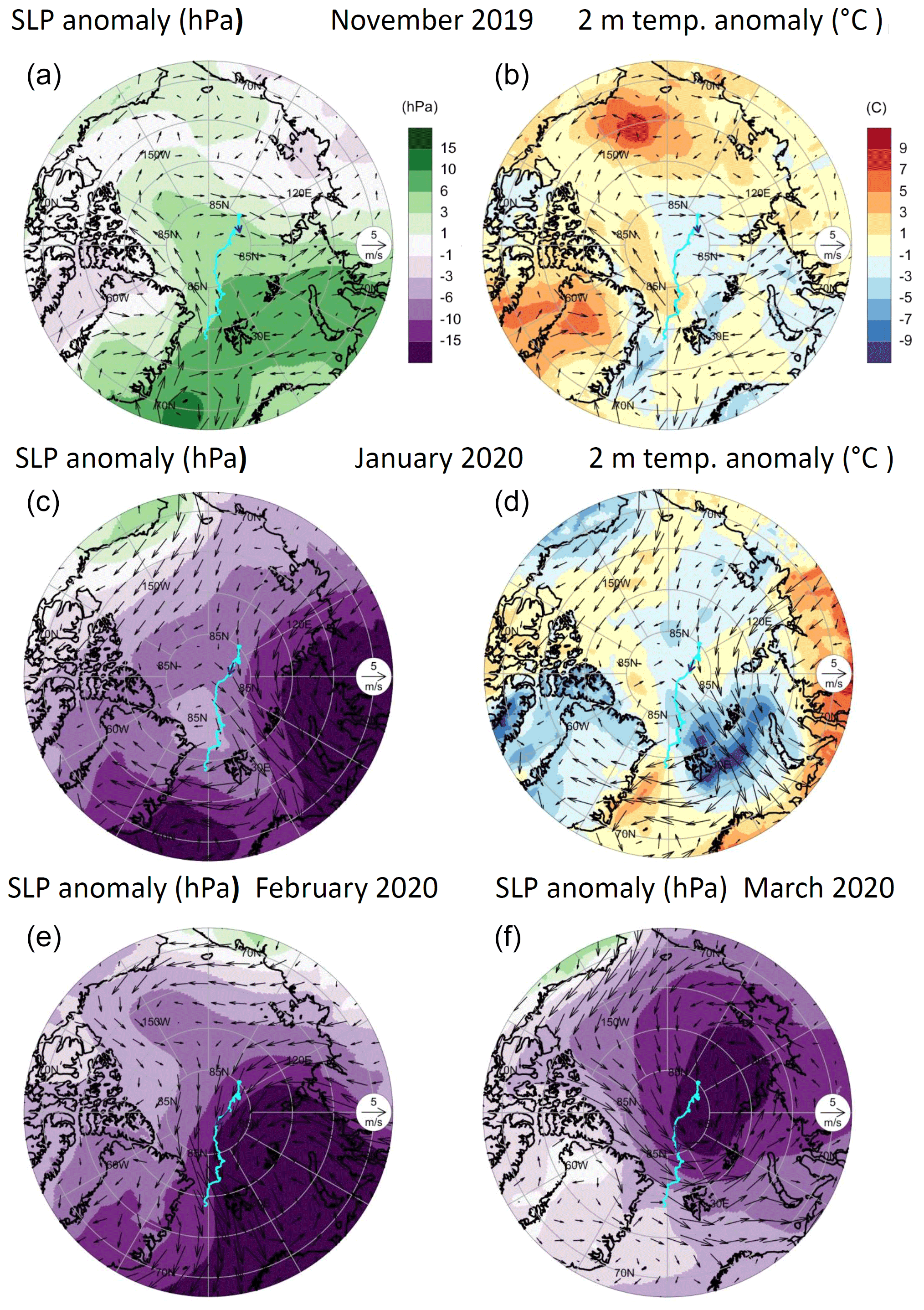
Figure 2Sea-level pressure anomaly (hPa) (a, c, e) and 2 m temperature anomaly (K) (b, d, f) for November 2019 (a, b) and January 2020 (c, d) compared to the 2010–2019 climate mean based on ERA5. Sea-level pressure anomalies (hPa) for February 2020 (a, c, e) and March (b, d, f) 2020 (e, f). Arrows display the direction and strength of 10 m atmospheric winds. Cyan lines indicate the MOSAiC ice floe track from October 2019 until August 2020. Small blue arrows indicate the location and drift of MOSAiC during the respective month.
The shift from a negative phase in November to the positive AO phase in January, February and March 2020 is displayed in Fig. 1. Figure S1 in the Supplement presents the PDFs of the daily AO indices for November and January–March (JFM) from 1979 until 2018/2019 (gray) in comparison to November 2019 (blue) and JFM 2020 (blue) with the prevailing positive AO index in 2020. Figure 2 displays the SLP anomaly and the 2 m temperature anomaly for November 2019 and January 2020 and the SLP anomalies for February 2020 and March 2020 compared to the mean for 2010–2019 based on ERA5 data. During November, the negative AO phase occurs with a higher-pressure anomaly over most regions of the Arctic Ocean and relatively warm temperatures in the Beaufort and Siberian seas. This pattern of near-surface atmospheric circulation coincides with low-level (10 m) winds from the southwest of Greenland and with an inflow of warm air masses into the western Arctic. During January 2020, a low-pressure anomaly developed over the eastern Arctic, along with a high-pressure anomaly over the western Arctic. This atmospheric flow configuration induced strong northerly winds from the cold Arctic Ocean to the BS and accelerated the southward drift of the MOSAiC ice floe in the Transpolar Drift. A regional cold-temperature anomaly developed in the northern part of BS. In February 2020, the low-pressure system stayed over the BKS and adjacent land regions and pushed sea ice into the BS, whereas the Kara Sea experienced southerly winds and thus warm anomalies. By March 2020, the low-pressure anomaly was located north of the Laptev Sea, inducing westerly wind anomalies that followed Arctic cyclone tracks in the BKS and keeping the cold air in the Arctic.
Besides the AO, the Arctic Dipole (AD) pattern is important for the Arctic circulation and sea ice motion (Wu et al., 2006; Cai et al., 2018; Watanabe et al., 2006; Zhang, 2015). In its positive phase, the AD pattern is connected with a negative pressure anomaly over the eastern Arctic and a positive pressure anomaly over the western Arctic, and leads to an acceleration of the Transpolar Drift, in agreement with Lei et al. (2016). Previous studies on the AD pattern in either summer (Cai et al., 2018) or winter (Wu et al., 2006) have often used a rather small domain (60–90∘ N or 70–90∘ N) and defined the AD pattern as the second EOF of monthly mean SLP fields. For these small areas, the domain boundaries do induce an artificial preference for particular pattern structures, as discussed by Legates (1993) and Overland and Wang (2010). Since neither EOF2 nor EOF3 of the abovedescribed analysis of the large domain 20–90∘ N revealed an AD pattern, an additional EOF analysis of monthly mean SLP over the smaller domain 60–90∘ N was performed over the same period (1979–2000) as before.
Figure S2 in the Supplement shows the first three EOFs and their daily indices. The first EOF again displays the AO pattern, and the daily indices over the MOSAiC period from November 2019 to May 2020 are highly correlated (0.95) with the AO index based on the EOF1 for the large domain (Fig. 1a). In this analysis, the AD pattern manifests itself as the third EOF, which indicates that the AD pattern is less stable than the AO pattern. The explained variances are 15 % for the second EOF and 13.6 % for the third EOF (AD). The positive AO phase from January to March 2020 is accompanied by a prevailing positive phase of the AD pattern (Fig. S2). The histogram of the daily AD indices for the period January to March 2020 indicates a higher variability of the AD index compared to the AO index (compare Fig. S1, right and Fig. S3 in the Supplement). Whereas the AO index remains positive from January to March 2020, the AD index shows a prevailing positive phase but with a smaller shift of the distribution towards positive values compared to the shift in the distribution of the AO index. The time series of the AD index reveals more positive values in January and March, but a shift to more neutral and negative values in February (see the time series for EOF3 in Fig. S2). This behavior of the AO and AD indices explains, to a large extent, the differences in the monthly mean SLP pattern over the Arctic for January, February and March, as displayed in Fig. 2.
Krumpen et al. (2021) analyzed shipborne observations of winds, air temperatures and sea-level pressures along the MOSAiC ice drift trajectory with ERA5 data for 2005–2020. Figure S4 in the Supplement compares the 10 m wind, 2 m temperature and sea-level pressure along the MOSAiC drift trajectory based on ERA5 data with the ERA5 climatology 2010–2019 applied in this study. The strongest deviations from the climatology occur during January–March 2020. In mid-February, a low surface pressure anomaly is connected to a strong synoptic cyclone event with values down to 985 hPa. This low-pressure anomaly is connected with warmer temperatures and higher wind speeds. In contrast, high pressure values at the beginning of March 2020 are connected with cold temperatures and lower wind speeds, indicating the important role of warm or cold advection in temperature changes.
Lei et al. (2016) investigated the sea ice motion from the central Arctic to the Fram Strait with ice-tethered buoys between 1979 and 2011 and showed that sea ice drift was mainly determined by near-surface winds. They detected an accelerated meridional sea ice velocity that followed the Arctic Dipole (AD) pattern, and a reduced meandering of the ice trajectories during the positive AD phase. The drift of the central MOSAiC Observatory was closely correlated with the ERA5 zonal and meridional components of the 10 m winds (blue and red curves in Fig. S5 in the Supplement). Compared to previous years, winds tended to have anomalies toward the Fram Strait, in particular in January, February and March 2020 (compare the red and black curves in Fig. S5, bottom), in line with corresponding sea-level pressure patterns (Fig. 2). Moreover, while the ice drift speed amounted to about 2 % of the 10 m wind speed on average, the drift component toward the Fram Strait was positively offset compared to the winds. The blue curve (ice drift towards the Atlantic) was positively relocated from the red curve (winds towards the Atlantic) over much of the year. In some months, the drift continued toward the Atlantic, even when the winds were temporarily blowing toward the Laptev Sea. In particular, from mid-February until the end of March, several short periods of wind toward eastern Siberia (negative values in Fig. S5, bottom) did not result in reversed drift; they only prompted the Transpolar Drift to slow (values close to zero in Fig. S5, bottom), likely due to the continued action of ocean currents and/or internal ice stress. From mid-June onwards, pronounced inertial motions were superimposed on the ice drift (Fig. S5), hinting at less concentrated sea ice (e.g., Gimbert et al., 2012). Covariability between the 10 m wind speed components and the sea ice velocity is visible during the positive-AO months of January–March 2020 (Fig. S5). The direct and accelerated MOSAiC drift towards the Fram Strait during January–March 2020 was a result of the positive AO phase (Fig. 1) accompanied by the prevailing positive AD phase (Fig. S2).
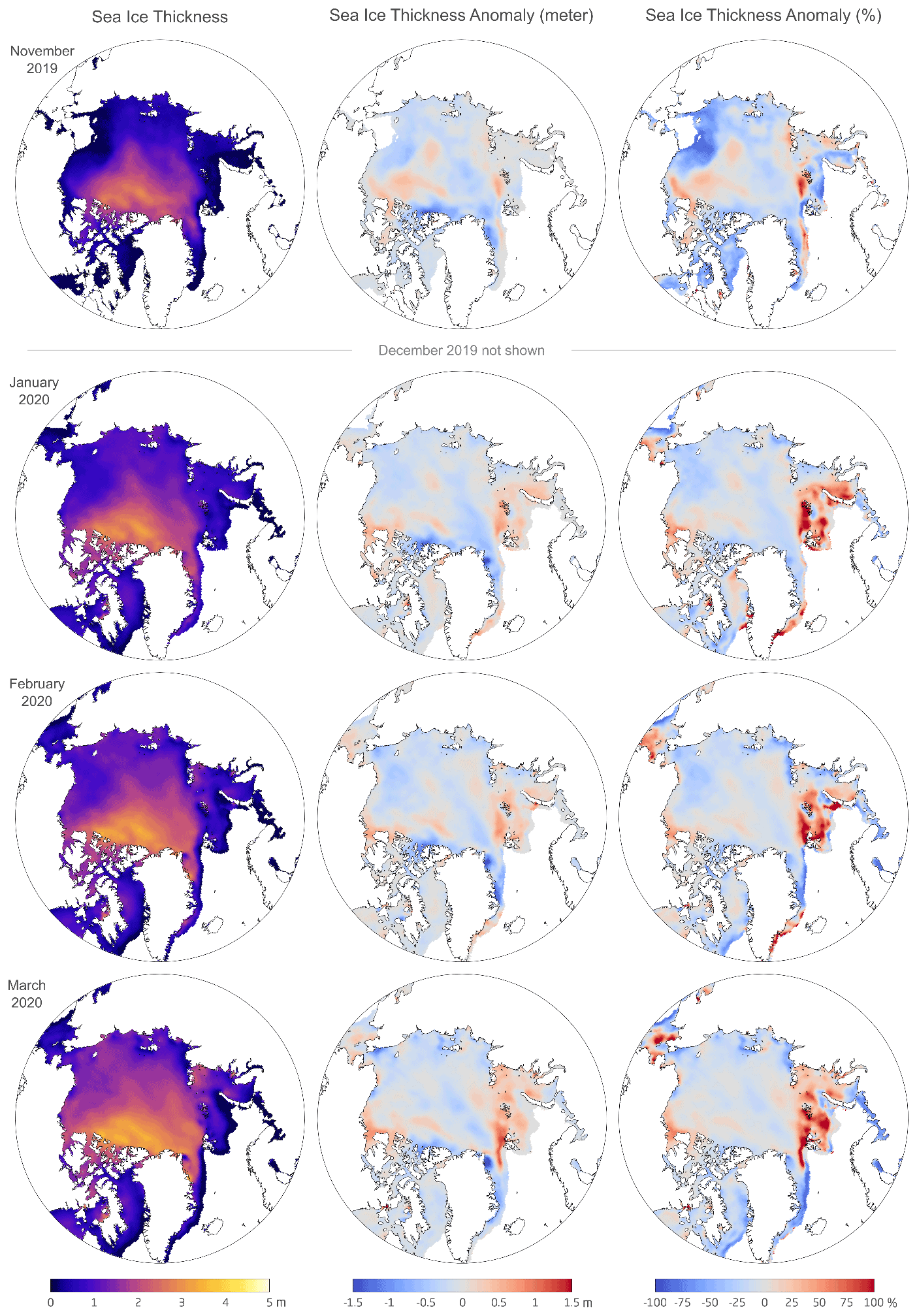
Figure 3Results based on CryoSat-2/SMOS satellite data analysis for sea ice thicknesses (left column) and anomalies in meters (middle column) and in percent (right column) from November 2019 (top row) through March 2020 (bottom row) (excluding December 2019). Note that values are given relative to the mean condition in the entire data record (2010–2019).
3.1.2 Sea ice thickness and extent
Sea ice thicknesses and anomalies from November 2019 through March 2020, based on CryoSat-2/SMOS satellite data analysis and compared to the mean condition in the entire data record (2010–2019), are presented in Fig. 3. The figure shows a regionally varying pattern of positive and negative sea ice anomalies. In November 2019, positive-thickness anomalies occurred in the Beaufort Sea (BS) and northeast of Spitsbergen. In the Bering Strait, a negative ice anomaly occurred. As early as December 2019 (not shown), weak sea ice anomalies developed in the BKS. In January 2020, a pronounced ice anomaly was visible in the BKS, which persisted with regional changes in the Kara Sea through February and into March 2020 when sea ice thickness increased west of Spitsbergen. Positive ice anomalies developed at the Bering Strait and the Canadian coast. In relative terms, the anomaly in the BKS is more significant, as it almost doubled the thickness in the first-year ice region, as seen in the relative sea ice thickness anomaly fields in the third column of Fig. 3. November 2019 was a month with a pronounced negative AO phase, whereas the months JFM 2020 were marked by a strong positive AO. Figure 3 shows enhanced sea ice anomalies in the BKS during JFM 2020. These sea ice anomalies occur at the same time as the persistent positive AO phase (Fig. 1). To understand the underlying thermodynamic and dynamic contributions to the observed sea ice thickness evolution, we now discuss simulation results from the fully coupled RASM model.
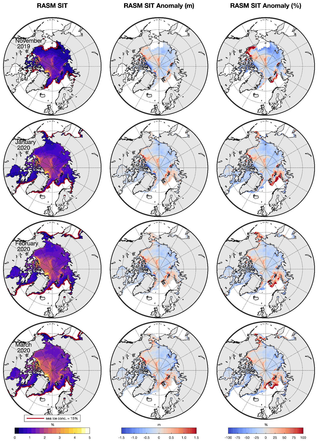
Figure 4Results based on RASM hindcast simulation for sea ice thicknesses (in meters, left column; black contour line represents a sea ice concentration of 15 %) and anomalies in meters (middle column) and in percent (right column) for November 2019 (top row), January 2020 (second row), February 2020 (third row) and March 2020 (bottom row). Note that values are given relative to the climate mean for 2010–2019.
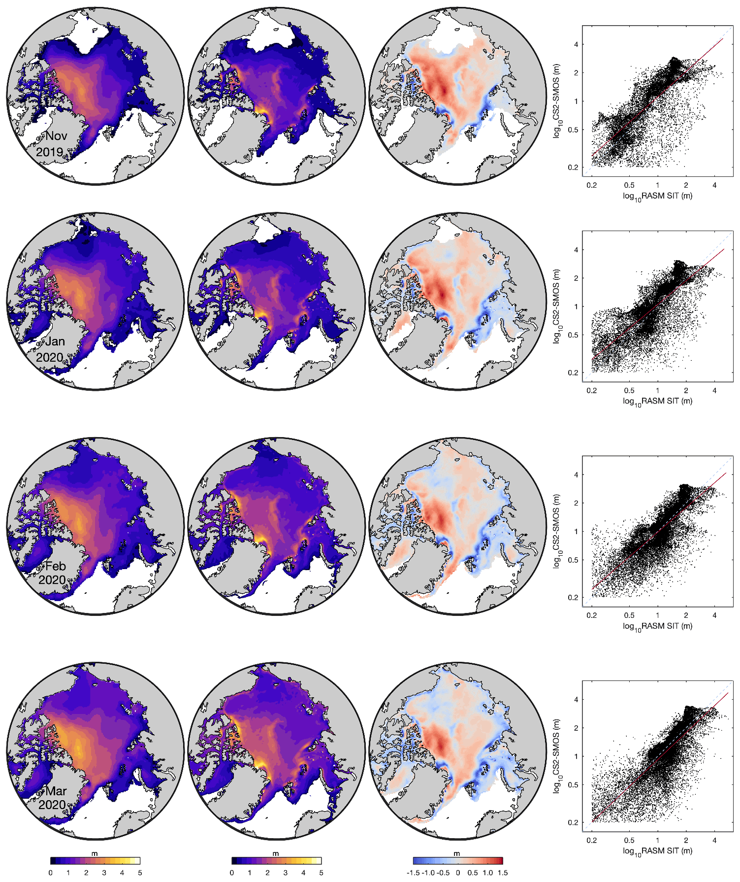
Figure 5Sea ice thicknesses (m) for November 2019 (top row), January 2020 (second row), February 2020 (third row) and March 2020 (bottom row), based on CryoSat2/SMOS (first column), RASM simulations (second column) and CryoSat2/SMOS minus RASM (third column). The fourth column shows scatterplots and the correlation between CryoSat2/SMOS data and RASM results.
3.2 Simulation of atmospheric and sea ice conditions in RASM
3.2.1 Model evaluation
Figure S6 in the Supplement presents the RASM-simulated atmospheric large-scale circulation for January 2020 (as an example), which compares well to the SLP anomalies in the positive AO phase shown in Fig. 1. The pronounced negative 2 m temperature anomaly observed in the BS in January 2020 (see Fig. 2) is also reproduced. The accurate simulation of this atmospheric circulation pattern is a result of grid-point nudging of the atmosphere above 500 hPa in RASM to the AO phase. The SLP and temperature anomalies simulated by RASM (Fig. S6) are associated with positive SIT anomalies in the BS and east of Spitsbergen (presented in the second and third rows of Fig. 4). The simulated ice-thickness anomalies for November 2019 and January, February and March 2020 are in qualitative agreement with the satellite-derived SIT anomalies for the same months (displayed in Fig. 3). The largest positive-thickness anomalies of between 1.0 and 1.5 m occur in the BS, along the northeastern Canadian coast and in the central Arctic Ocean. In all other regions, and especially over the Bering Strait and the Siberian Sea, the sea ice is thinner than the 2010–2019 mean. The RASM simulations (Fig. 4) also exhibit positive SIT anomalies for the Arctic Ocean northwest of Greenland that are not found in the CryoSat-2/SMOS-derived SIT anomalies (Fig. 3). A more in-depth comparison of the SITs for November 2019 and JFM 2020 (Fig. 5) indicates that there is thicker ice stretching further into the central basin from Greenland in the CryoSat2/SMOS-derived SIT compared to the RASM. In the BKS, the Laptev Sea and the Bering Strait, the RASM simulations indicate thicker sea ice ranging up to 1 m compared to the satellite-derived data. The SIT simulations in RASM were independently compared with other coupled and uncoupled model systems in a quality control by Roberts et al. (2018) and found to be in good agreement with the limited observations. A high correlation between CryoSat2/SMOS-derived SIT and RASM simulations is visible in the rightmost column of Fig. 5. The differences in SIT observed in Fig. 5 may be partly connected to the impact of surface roughness on the radar freeboards and the retrieval algorithms, as discussed by Landy et al. (2020).
The merged CryoSat-2/SMOS SIT data are dominated by the CryoSat-2 radar altimeter contribution in areas with multi-year sea ice. The radar freeboard in sea ice radar altimetry describes the height of the ice surface above local sea level as perceived by a radar altimeter. It differs from the sea ice freeboard – the actual height of the ice surface – by a correction that requires prior knowledge of the snow depth and density. The purpose of this correction is to remove the impact of the slower wave propagation speed of the radar pulse within the snow layer on the radar range and thus ice surface elevation. The corrected radar freeboard is then converted to the sea ice thickness using information on the densities of sea ice, ocean water and snow and by estimating the depth of snow that has accumulated on the ice surface based on climatological values (Hendricks and Ricker, 2020). In Landy et al. (2020), it is demonstrated that sea ice surface roughness may cause a systemic radar freeboard uncertainty, which represents one of the principal sources of pan-Arctic SIT uncertainty. In the CryoSat-2 retrieval algorithm of the CryoSat-2/SMOS SIT data set, this systemic bias might contribute to the higher CryoSat-2/SMOS thicknesses in the central Arctic (specifically, north of the Canadian Archipelago) with respect to RASM in Fig. 5. However, this assertion does not consider other systemic uncertainties present in the CryoSat-2 retrieval, such as the underestimation of the sea ice density for multi-year ice in recent years (Jutila et al., 2022), which might compensate for the radar freeboard bias to an unknown extent. In comparison to other SIT data sets, CryoSat-2/SMOS also yields thicker ice in the central Arctic compared to ICESat-2 estimates. Although the differences are within the range of SIT uncertainty resulting from different retrievals, they are still an indication of SIT overestimation by CryoSat-2/SMOS.
The 50 % threshold method was used to construct Fig. 5, and this threshold leads to thicker ice in the central Arctic compared to the ICESat-2 estimates. Landy et al. (2020) showed that variable ice surface roughness contributes a systematic uncertainty in sea ice thickness of up to 20 % for first-year ice and 30 % for multi-year ice, and represents one of the principal sources of pan-Arctic sea ice thickness uncertainty.

Figure 6(a) Target diagram of the normalized bias and the normalized unbiased root-mean-square difference (uRMSD) and (b) Taylor diagram of the normalized standard deviation and the correlation between the RASM sea ice thickness simulations and CryoSat2/SMOS data from November 2019 to March 2020. The filled black square indicates the reference (REF) value, i.e., a perfect model.
RASM's skill is assessed by comparing the root-mean-square difference (RMSD) against observational data. Figure 6a shows a target diagram (Joliff et al., 2009) displaying the unbiased RMSD (uRMSD; x axis) and bias (y axis) for monthly SIT on a single plot, i.e., RMSD2= bias2+ uRMSD2. These quantities are normalized by the standard deviation of the CryoSat2/SMOS SIT. Figure 6b is a Taylor diagram (Taylor, 2001) that shows the relative skill of RASM with respect to CryoSat2/SMOS. It provides an additional set of statistics in uRMSD by displaying the correlation and the ratio of the standard deviation between the RASM and CryoSat2/SMOS SITs for each month from November 2019 until March 2020.
Table 1Comparison between the CryoSat2/SMOS satellite data and RASM simulations in the mean (Mean) and standard deviation (SD) of the sea ice thickness from November 2019 until March 2020, along with the corresponding correlation, bias and root-mean-square error (RMSD) values.

A high correlation between satellite- and model-estimated SIT is observed for all of the considered months (Fig. 5, rightmost column). The bias and root-mean-square difference for RASM (Fig. 6a) and the standard deviation and correlation (Fig. 6b) relative to CryoSat2/SMOS for each month from November 2019 until March 2020 with respect to sea ice thickness show a high correlation (above 0.7) for all months and a low standard deviation of the model simulations from the satellite-based SIT. A comparison between the CryoSat-2/SMOS data and the RASM hindcast simulations in the monthly mean and standard deviation of the sea ice thickness from November 2019 until March 2020, along with the corresponding correlations, biases and root-mean-square differences, is shown in Table 1; high correlations of between 0.84 and 0.86 and low domain-averaged biases are seen. The domain-averaged bias is the difference between RASM and satellite data in all sea ice regions with boundaries at the DS (Davis Strait), FS (Fram Strait), BSO (Barents Sea Opening) and BS (Bering Strait), as defined in Fig. 12.
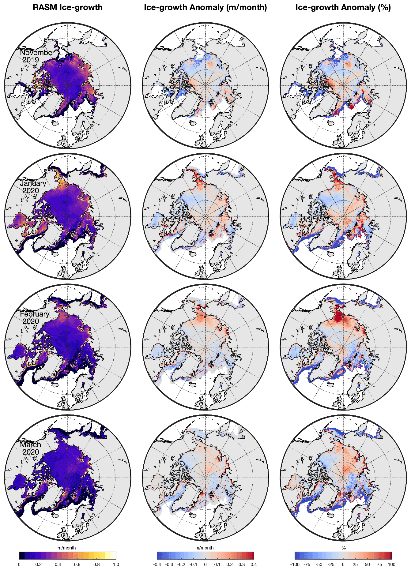
Figure 7The integrated sea ice growth (m/month; left) and sea ice growth anomalies in m/month (middle) and in percent (right) for November 2019 (top row), January 2020 (second row), February 2020 (third row) and March 2020 (bottom row) from the RASM hindcast simulation. Note that values are given relative to the climate mean for 2010–2019.
3.2.2 Interpretation of the positive sea ice anomaly in the BS
The integrated sea ice growth anomalies of RASM (Fig. 7) compared to the mean for 2010–2019 indicate regionally varying ice growth over the whole Arctic Ocean during polar night conditions and regions of enhanced ice growth, which start northwest of Greenland and along the sea ice border in the eastern Arctic in November 2019. In January 2020, strong ice growth takes place in the BKS, the Siberian Sea and the Bering Strait. In February 2020, the strongest ice growth anomalies are simulated over the Beaufort and Chukchi seas, and in March 2020 they are over the mid-Arctic Ocean, parts of the BS and the east coast of Greenland. In February and March 2020, weaker sea ice growth is modeled in the Laptev Sea, east of Greenland and in the Davis Strait.
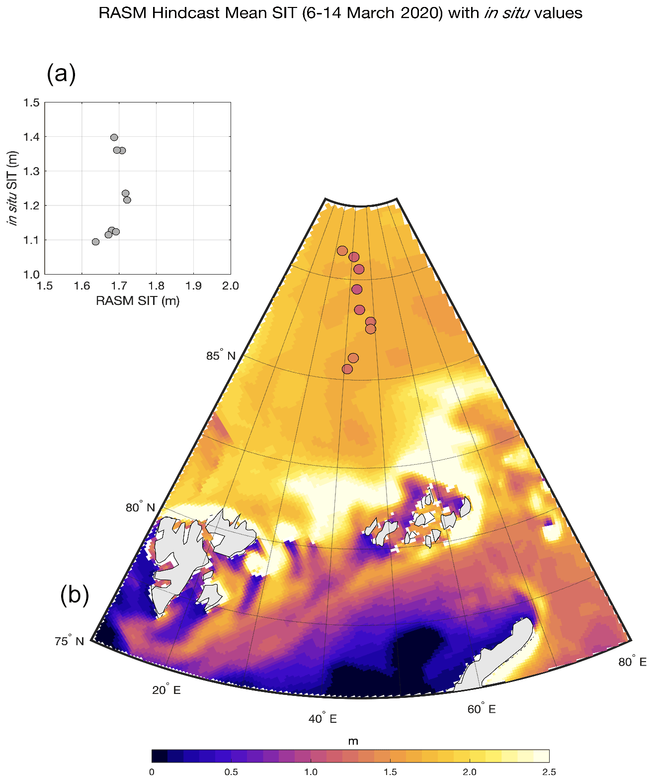
Figure 8Panel (a) compares the in situ sea ice thickness measurements (m) with the corresponding RASM simulations at all points indicated by circles in (b), which shows the mean sea ice thickness (m; shading) from the RASM hindcast simulation during 6–14 March and daily EM (Electromagnetic induction) ice thickness measurements (m; circles) taken on the RV Kapitan Dranitzyn from 6 to 14 March 2020.
The EM ice thickness measurements undertaken onboard the Russian icebreaker RV Kapitan Dranitzyn during the MOSAiC resupply voyage between 6 and 14 March 2020 indicated heavy sea ice conditions between 84 and 88∘ N in the BS. Mean daily modal thicknesses are compared to the mean RASM simulations between 6 and 14 March 2020 in Fig. 8. The ship-based measurements ranged between 1.3 and 1.5 m and are 0.3–0.5 m thinner than those from RASM. The ship-based sea ice thickness is also 0.3–0.4 m thinner than what was observed in ground-based measurements at the MOSAiC ice floe (not shown), where modal thicknesses between 1.7 and 1.8 m were measured. The main bias of the EM ship-based measurements is connected to the difficulty involved in calibration on the ramming icebreaker. The frequent ramming operations of the ship as it makes little progress over the undisturbed heavy ice make processing and filtering of the ship-based measurements challenging. However, the RASM results would agree more closely with observations if ∼0.4 m were to be added to the ship-based data. Consequently, the regional gradients in both data sets with thinner ice to the south are also well described. The movement of the RV Kapitan Dranitzyn to the RV Polarstern in the sectors of the BS in the Arctic Basin in February 2020 and March 2020 was carried out under severe ice conditions with thick first-year and second-year ice. The movement of the supply vessel slowed down significantly due to the absence of extensive leads in the meridional direction and compression (especially in February 2020 on the way to the RV Polarstern). Large sea ice leads were predominantly oriented in the zonal direction as a result of the positive AO. Compression weakening and the local fracture system allowed RV Kapitan Dranitzyn to gradually move forward towards RV Polarstern. Sea ice leads in the infrared channel of NOAA-20 satellite pictures from 5 March 2020 with a resolution of 375 m point to a more zonal orientation due to the low-pressure systems connected to the positive AO phase (Fig. 9). A snapshot of the divergence of the sea ice on 5 March 2020 from the RASM simulations (Fig. 9b) shows several leads in the BS and north of it that are similarly oriented to leads in the NOAA-20 image (Fig. 9a).
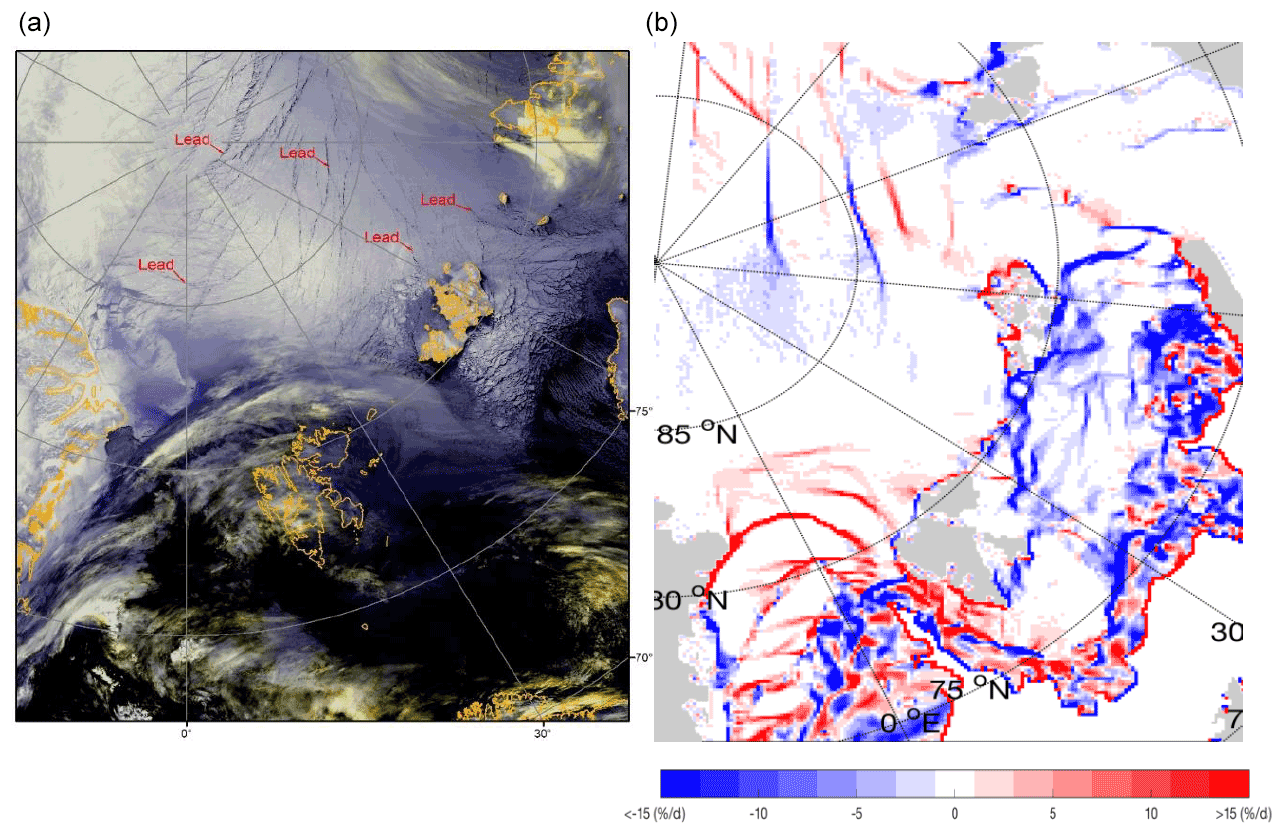
Figure 9(a) Sea ice lead structures in data taken on 5 March 2020 from infrared channel 5 of the NOAA-20 satellite with the highest possible resolution (375 m), with the identification of leads. These data were obtained using the VIIRS instrument (Visible/Infrared Imager Radiometer Suite) installed onboard the NOAA-20 satellite. (b) Daily mean sea ice divergence (% d−1) on 5 March 2020 in the RASM simulation. No data manipulation was done except for daily averaging.
Comparison of Figs. 4 and 7 indicates that positive sea ice growth anomalies in the BS occur in the region of positive-thickness anomalies during JFM 2020 as a result of enhanced ice growth due to colder temperature anomalies in this area (Figs. 2 and S6 in the Supplement). The temporal development of the ice anomalies shows rather good agreement between the satellite data and the RASM simulations (Figs. 3 and 4), especially in the BS region. The variety of processes and their interplay make it difficult for the coupled model simulation to reproduce the observed sea ice distribution and its trend in all geographical regions over the Arctic Ocean. Ice thickness anomalies are influenced by deformation parameters, e.g., divergence/convergence and shear, commonly generated in response to strong and/or persistent winds. Onarheim et al. (2015) demonstrated that changes in surface wind stress may explain 78 % of the sea ice extent variance in the BS. Oceanic heat transports are another essential driver of the ice distribution. Variability of oceanic heat transports and surface winds captures most of the sea ice variance in the BS. Momentum exchange due to turbulent atmospheric processes controls sea ice motion. Divergence generates open water areas where new sea ice growth may occur. Convergence leads to the formation of pressure ridges, and the SIT distribution in a region is influenced by the number and thickness of ice ridges present.
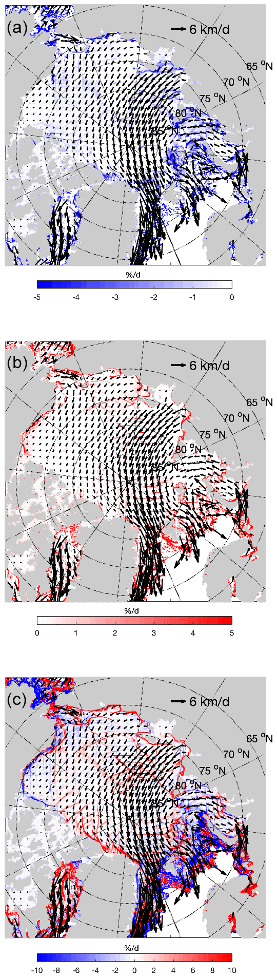
Figure 10Sea ice anomalies calculated from the RASM hindcast simulation for January–March (JFM) 2020 compared to the RASM climate mean for JFM 2010–2019 for negative divergence (a; blue shading represents less divergence) and positive divergence (b; red shading represents more divergence). Panel (c) displays ice shear anomalies (% d−1). The mean velocity vectors for the same period of JFM 2020 are overlaid in each plot.
The RASM-simulated positive and negative ice divergence anomalies and the ice shear anomaly for the JFM 2020 mean compared to the JFM 2010–2019 mean, together with the Transpolar Drift in km d−1, are indicated by black arrows in Fig. 10. In all three plots, the Transpolar Drift in km d−1 is indicated by thick black arrows. Longer vector arrows (black) in the Davis Strait, the east coast of Greenland and the BS indicate individual grid cells with very different drifts. Blue colors in Fig. 10a indicate regions with reduced convergence, and red colors in Fig. 10b indicate those with enhanced divergence. These grid cells likely reflect the free drifting of thinner sea ice in marginal ice zones, where the impact of atmospheric wind forcing on the drift ice is much less limited compared to when the drift occurs within pack ice.
The sea ice drift is a result of near-surface wind fields, which determine sea ice deformation, as described by, e.g., Spreen et al. (2011). Sea ice momentum changes are a result of air–ice and ice–ocean stresses, as discussed by, e.g., Martin et al. (2016).
Model deficits, which occur on daily timescales, drive differences in surface energy fluxes and hence sea ice growth and melt, and result in biases with respect to two-way feedbacks between sea ice area and thickness and sea ice growth and melt. To reduce the complexity of the feedbacks involved, we focus here on seasonal averages.
Negative ice divergence anomalies occur in the Fram Strait and the BS between Spitsbergen and Novaya Zemlya, and are displayed in Fig. 10a. Positive ice divergence anomalies are present in the Fram Strait and the west coast of Spitsbergen and are presented in Fig. 10b. This region also shows strong positive and negative values for the ice shear anomaly in Fig. 10c, which indicates a strong dynamic impact on sea ice formation and deformation in the BKS region. Reduced divergence, which corresponds to enhanced convergence, appears in a belt between West Greenland and the Kara Sea. In areas close to the ice edge, positive ice shear coincides with positive sea ice concentration anomalies, since there is more ice than usual there. The ice divergence anomalies are weaker and occur in the region of strongest sea ice growth, whereas ice shear processes due to wind stresses in Fig. 10c indicate positive anomaly values. The sea ice thickness anomalies in the BS region, where negative temperature anomalies occurred, are a result of wind stresses that enabled ice growth or ice deformation. Atmospheric surface wind stresses impact sea ice deformation, and the 10 m wind vectors show strong wind components from the north in the region east of Spitsbergen (see Fig. 2). The positive AO phase and the near-surface winds during JFM 2020 may be connected to an intensified and northward-shifted Atlantic storm track, as discussed by Serreze et al. (1997), Nie et al. (2008) and Inoue et al. (2012).
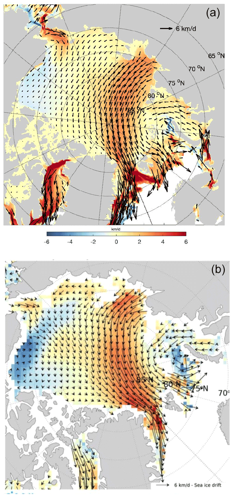
Figure 11RASM simulations of the sea ice velocity anomaly (a) and the satellite-derived sea ice velocity anomaly (km d−1) (b) for January 2020 to March 2020 compared to the climate mean for 2010–2019. The figures were plotted using IDL (Exelis Visual Information Solutions, Inc.).
3.2.3 Transpolar sea ice drift
The model-simulated sea ice velocity anomaly (Fig. 11, top) and satellite-derived sea ice velocity anomaly (Fig. 11, bottom) in km d−1, as computed from OSI-SAF low-resolution sea ice motion data during January–March 2020 and compared to the climate mean for 2010–2019, indicate strong acceleration of the Transpolar Drift during the MOSAiC winter, with intensified speeds of up to 6 km d−1. The Ocean Sea Ice Satellite Application Facilities (OSA-SAF) deliver satellite-derived scatterometer winds, sea surface temperatures and sea ice surface temperatures, radiative fluxes, sea ice concentrations, edges, types and sea ice drifts. The black arrows over the reddish shading in the eastern Arctic indicate the Transpolar Drift. Longer black arrows in the Davis Strait, the east coast of Greenland and the BS indicate the free drift of grid cells within marginal ice zones.
This drift is in general agreement with the 10 m winds displayed for January, February and March 2020 and the low-pressure anomalies presented in Fig. 2. The centers of the persistent low-pressure systems over the Arctic Ocean corresponding to the positive AO phase changed their positions during JFM 2020. In March 2020, the center moved toward Siberia, impacted the ice drift velocities in the BS region, and contributed to the increased sea ice thickness in the region around Spitsbergen. The low-pressure anomaly in March 2020 strengthened the drift towards the BS. Sea ice growth in the BS was caused by the combined effect of thermodynamic growth due to the colder temperatures there and dynamic SIT changes related to the positive AO phase and altered wind stresses, which affect the ice divergence. The simulated sea ice velocity anomalies agree well with the satellite-derived sea ice velocity anomalies, especially over the eastern part of the Arctic Ocean (Fig. 11). Over the Beaufort Sea and the western part of the Arctic Ocean, the sea ice drift in the RASM simulations is underestimated, and the direction differs from the satellite-derived data.
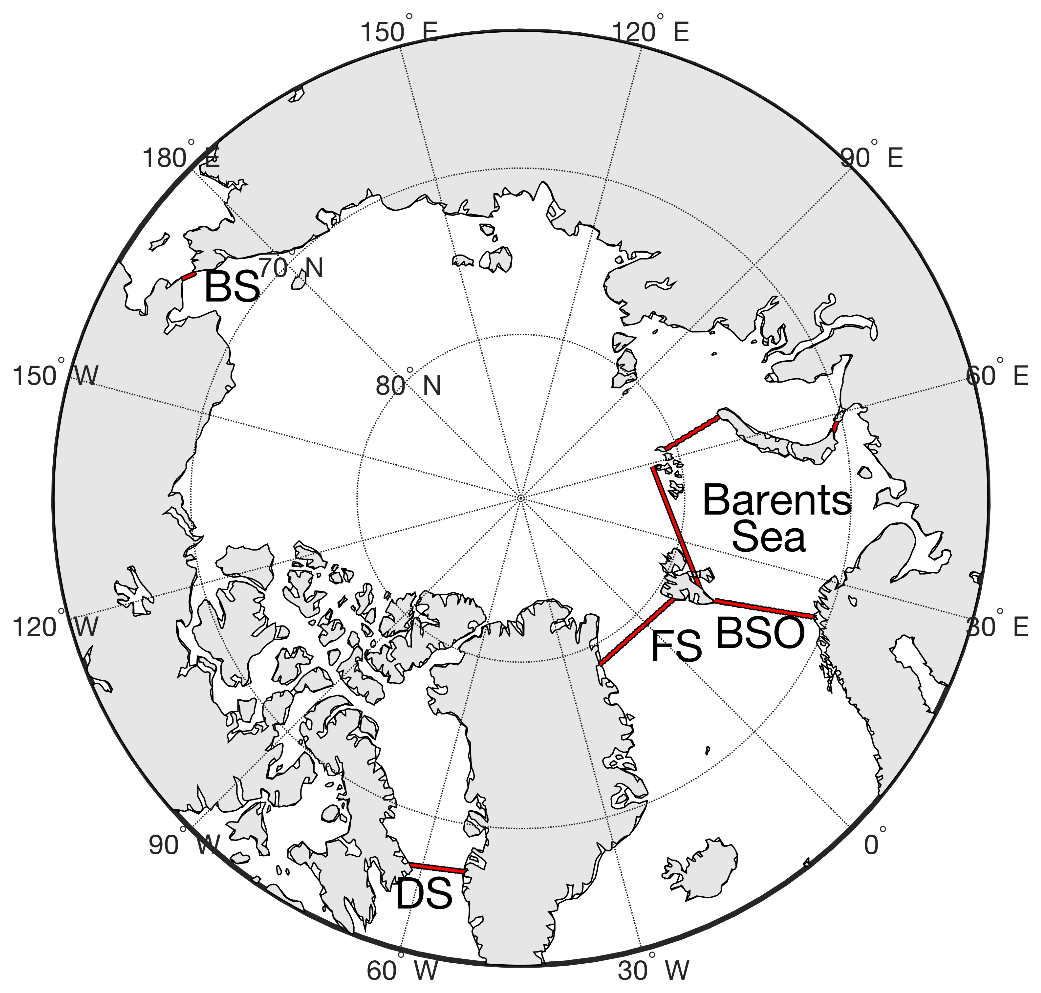
Figure 12The pan-Arctic and Barents Sea domains used for the computation of the sea ice volume tendencies shown in Fig. 13.
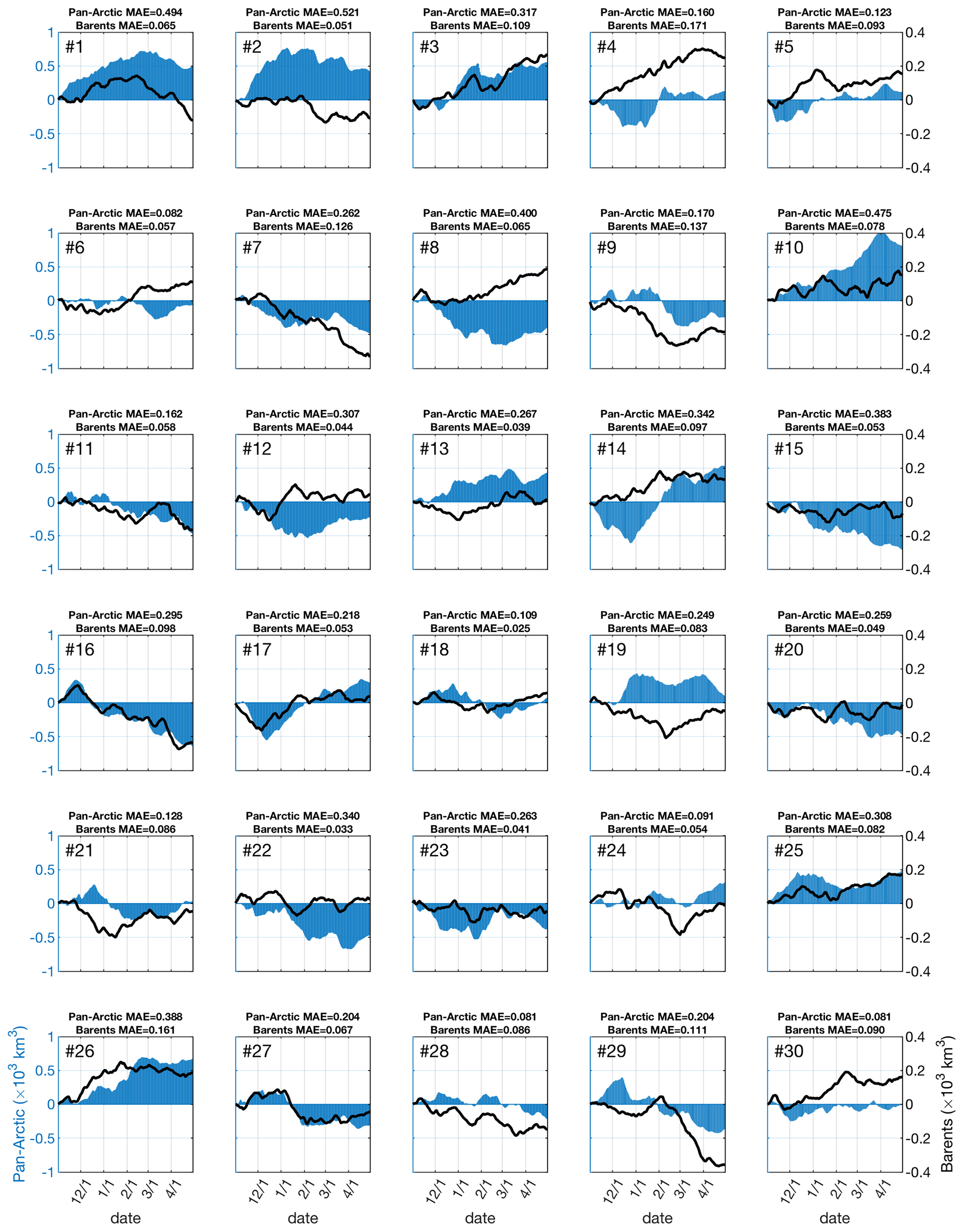
Figure 13Temporal evolution of the simulated mean absolute difference in sea ice volume (in 103 km3) from the ensemble mean for 30 ensemble members of RASM integrations from 1 November 2010 until 30 April 2020 in forecast mode for the pan-Arctic domain (blue) and the BS domain (black lines). Note the different y-axis scales used for the pan-Arctic (left) and BS (right) domains in the panels.
3.2.4 Internal variability
Previous work by Ding et al. (2019) and Nie et al. (2019) emphasized the importance of internal climate variations for the AO phase shifts. Here, we examine related regional sea ice variations in the pan-Arctic and BS domains (Fig. 12) with the nudged AO in ensemble forecasts. The pan-Arctic domain covers the whole Arctic Ocean, with borders at the Bering Strait (BSr), the Fram Strait (FS), the Barents Sea Opening (BSO) and the Davies Strait (DS). The temporal evolution of the mean absolute difference (relative to the ensemble mean) in the simulated pan-Arctic and BS sea ice volume for the RASM 30-member ensemble 6-month forecast simulations from 1 November 2019 through 30 April 2020 is shown in Fig. 13. The ensemble members were all initialized with the same sea ice and ocean conditions and on the same date, but were then forced by different NCEP Climate Forecast System (CFSv2) global forecasts initialized 24 h apart at 00:00 between 1 and 31 October 2019. The 30-member RASM ensemble was forced with different lateral boundary conditions from a 9-month forecast of the NCEP Climate Forecast System, applying linear nudging of the temperature and the zonal and meridional wind above 500 hPa. The differences among the 30 ensemble members for the pan-Arctic domain are in the range of 1000 km3 and show significant positive or negative departures from the ensemble mean volume. The results presented in Fig. 13 point to large internally generated variability of the pan-Arctic and BS sea ice volume changes in the coupled regional system and remote impacts from the mid-latitudes. Differences in modeled sea ice volume vary significantly between the pan-Arctic and the BS regions and can even have opposite signs, as seen for ensemble members 2 and 8, for example. The sea ice evolution differs for all 30 ensemble members, e.g., ensemble members 1, 2, 3, 10, 13, 19, 25 and 26 show positive sea ice volume differences of different strengths during winter 2019/20 in the pan-Arctic domain, whereas ensemble members 7, 8, 9, 15, 16, 22 and 23 show negative ice volume differences of various strengths. In the BS, ensemble members 2, 4, 8, 12, 19 and 30 show different ice volume trends in comparison to those in the pan-Arctic domain.
To quantify the underlying mechanisms for the Arctic ice volume differences and their temporal evolution, we analyze two integrated quantities that are readily available from the CICE sea ice model, i.e., dynamic (DVT) and thermodynamic (TVT) volume tendencies. These are defined as the net change in ice volume per unit area and per unit time (in m s−1) due to the integrated effects of dynamics/transport and thermodynamics, respectively (CICE Consortium, 2021, https://cice-consortium-cice.readthedocs.io/_/downloads/en/master/pdf, last access: 27 September 2021). Thermodynamic ice volume tendencies capture the temporal development of the ice thickness structure based on energy conservation principles, whereas dynamic tendencies determine the motions of sea ice based on the conservation of momentum. As per its definition, the DVT integrated over the total area of Arctic sea ice cover must be equal to zero. While observational estimates of these quantities are very limited in terms of both locations and dates, the evolution of an area-integrated temporal model of them provides useful information with regard to the mechanisms driving the sea ice state. In addition, an approach with a relatively large ensemble size allows probabilistic estimates of their importance to be obtained.
Compared to the hindcast values (yellow bars), the tendencies in different months vary for both the pan-Arctic and BS domains. In February 2020 and March 2020, the mean sea ice volume tendencies reach 73–58 km3 d−1 in the pan-Arctic domain. The standard deviation remains similarly strong from November 2019 to February 2020 and becomes weaker in March 2020. The thermodynamic sea ice volume tendencies in the BS during January 2020 and February 2020 are in the range of 6 km3 d−1, and are above 4 km3 d−1 during March 2020.
Standard deviations in the BS are highest in December 2019. In addition, we show the dynamic ice volume tendencies (DVT) in the BS (note that the pan-Arctic dynamic ice volume tendencies are zero by definition), which are weaker and indicate a sea ice decline in most ensemble members and during all months. Only six ensemble members show positive dynamic ice volume tendencies during January and February, but eight members did so in March. The hindcast simulation indicates that BS dynamic tendencies were near to zero in January, negative in February, but positive in March 2020.
The statistical properties of thermodynamic sea ice volume tendencies are based on differences in daily values. These tendencies for the pan-Arctic and BS domains and dynamic ice volume tendencies for the BS region from November 2019–March 2020 are shown in Figs. S7–S9 in the Supplement. The strong deviations due to internally generated variability in Arctic sea ice growth and dynamic ice deformations are visible. Ensemble members 2 and 8 have been selected to represent the maximum and minimum ice volume differences, respectively, for the whole pan-Arctic domain. However, those two ensemble members are not representative of the smaller BS domain, which is why ensemble members 4 and 9 were selected. In the RASM hindcast, the pan-Arctic thermodynamic sea ice volume tendencies increase due to ice growth from November 2019 until January 2020. The differences between the hindcast and the four selected forecast simulations (2, 4, 8 and 9) are large during all the months from November 2019 until February 2020, and can reach ∼20 km3 d−1, or ∼600 km3/month. The thermodynamic ice volume tendencies in BS for the same four ensemble members (2, 4, 8 and 9) are in the range of 3 km3 d−1 or ∼90 km3/month.
The SLP anomalies in November 2019 and January 2020 (Fig. S10 in the Supplement) for the hindcast simulation, pan-Arctic ensemble member 2 with a positive sea ice anomaly in Fig. 13, and pan-Arctic ensemble member 8 with a negative sea ice anomaly in Fig. 13 have been selected. The SLP pattern (Fig. S10) for ensemble member 8 shows a strong low-pressure anomaly in January over Siberia, and that for ensemble member 2 shows a high-pressure anomaly in January over the Arctic Ocean. The 500 hPa geopotential heights for the RASM hindcast and the two ensemble members (not shown) indicate a pronounced barotropic structure in the troposphere and emphasize the diverging development of the pressure, temperature and geopotential patterns and the important role of internally generated variability in sea ice formation, as pointed out by Ding et al. (2019). Compared to the brevity of atmospheric timescales (i.e., daily), the longer timescales of ocean and sea ice processes provide memory effects for seasonal sea ice forecasts, but the large atmospheric variability connects sea ice predictability to atmospheric wind predictions for up to 10 d, as discussed by Inoue (2021), and sets inherent limits on seasonal sea ice predictions, as pointed out by Serreze and Stroeve (2015).

Figure 14Thermodynamic sea ice volume tendencies (km3 d−1) for all 30 ensemble members and the RASM hindcast simulation (yellow) for the pan-Arctic (left column) and the Barents Sea (middle column) along with the combined ice-growth and ice-melt terms and the dynamic sea ice volume tendencies (km3 d−1) for the Barents Sea (right column). Four individual ensemble forecast members are selected: members 2 (red), 4 (orange), 8 (light blue) and 9 (dark blue).
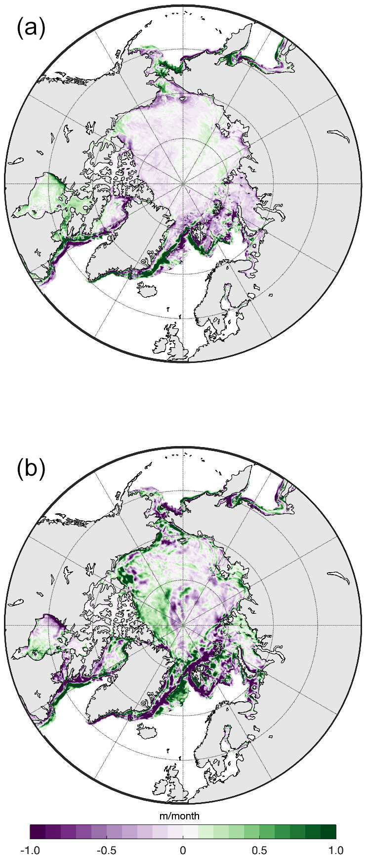
Figure 15Differences between RASM ensemble members 2 and 8 in accumulated (a) thermodynamic (m/winter) and (b) dynamic sea ice volume tendencies (m/winter) for JFM 2020.
The differences in thermodynamic and dynamic ice volume tendencies per model grid cell shown in Fig. 15 represent the sea ice redistribution between RASM pan-Arctic ensemble member 2 (positive ice difference in Fig. 13) and pan-Arctic ensemble member 8 (negative ice difference in Fig. 13). The largest sea ice volume increase occurs for both ensemble members in the BKS and on the northwest side of Greenland (Fig. 15). In both ensemble members, the thermodynamic ice growth is in the range between 0.5 and 1 m/winter, with more enhanced ice growth occurring in the Laptev Sea (not shown). The differences between the two forecast ensemble members are in the range of up to −0.5 m in the BKS and up to 0.3 m over the Arctic Ocean. The accumulated winter (JFM 2020) ice volume tendencies under dynamic and thermodynamic drivers are largest in the BS. Bigger ice volume differences occur northwest of Greenland, with differences of more than 0.5 m occurring during the winter. The pan-Arctic sea ice volume represents the coupled system response to large-scale forcing and is a better diagnostic of different sea ice regimes among ensemble members, since the sea ice extent and sea ice area are relatively similar in winter. Compared with the dynamic contributions, thermodynamic growth processes (Fig. 15) lead to the greatest differences between the two ensemble members in the BKS and at the ice edge region around Spitsbergen and Greenland. Thermodynamic and dynamic processes produce similar peak differences. Although the greatest differences occur at the ice edge regions, remarkable changes in the inner Arctic northwest of Greenland are visible, and the sea ice volume in this region is determined to a large extent by dynamic processes. For the BS, the strengths of the thermodynamic and dynamic contributions were determined using ensemble simulations (Fig. 14). A big spread in the strengths of thermodynamic and dynamic drivers of the sea ice state occurs, in agreement with West et al. (2021).
3.2.5 Case study of positive and negative AO winters
To contrast the sea ice conditions and the regional processes and feedbacks for positive and negative AO winters, we compare the RASM hindcast results for the MOSAiC winter 2020, when there was an exceptionally positive AO phase, against the exceptionally negative AO winter of 2009/2010. Figure S11 in the Supplement displays the time series of the AO index from October 2009 until May 2010, which indicates that there was a weakly positive AO phase in November 2009 and the strongest negative AO phase during the last 60 years in winter 2010 (L'Heureux et al., 2010). As discussed, e.g., by Zhao et al. (2019), the AO phase is closely related to sea ice variability over the Arctic Ocean. Surface heat fluxes in the coupled Arctic climate system in winter are influenced by different positive and negative feedbacks such as vertical ocean convection, atmospheric turbulence, latent heat and cloud formations, longwave radiation, oceanic currents, Arctic storms and atmospheric circulations, and can be considered an integrated quantity that is related to all these processes. This regional approach has obvious limits; e.g., Gong et al. (2020) showed the existence of a hemispheric planetary wave train that propagates from the subtropics through mid-latitudes and into the Arctic and back, recharging and amplifying over the Arctic through anomalous latent heating over the Greenland Sea and BKS.
Figure S12 in the Supplement shows the results of RASM simulations of SLP and 2 m temperature for January 2010, which represents a negative AO phase, given atmospheric nudging above 500 hPa in RASM. The nudging of the coupled RASM to different AO phases allows an efficient, albeit coarse, diagnosis of differences between the surface heat fluxes for the two AO phases. Comparison of Fig. S12 with Fig. S6 indicates an inverse temperature anomaly pattern between the western and eastern Arctic for positive and negative AO winters. Under positive AO conditions in winter (Fig. S6 shows January 2020 as an example), negative temperature anomalies occur over the eastern Arctic and positive anomalies occur over the Canadian Basin in the western Arctic. During the negative AO winter conditions in January 2010 (Fig. S12), the eastern Arctic reveals weak positive temperature anomalies and the western Arctic shows negative temperature anomalies.
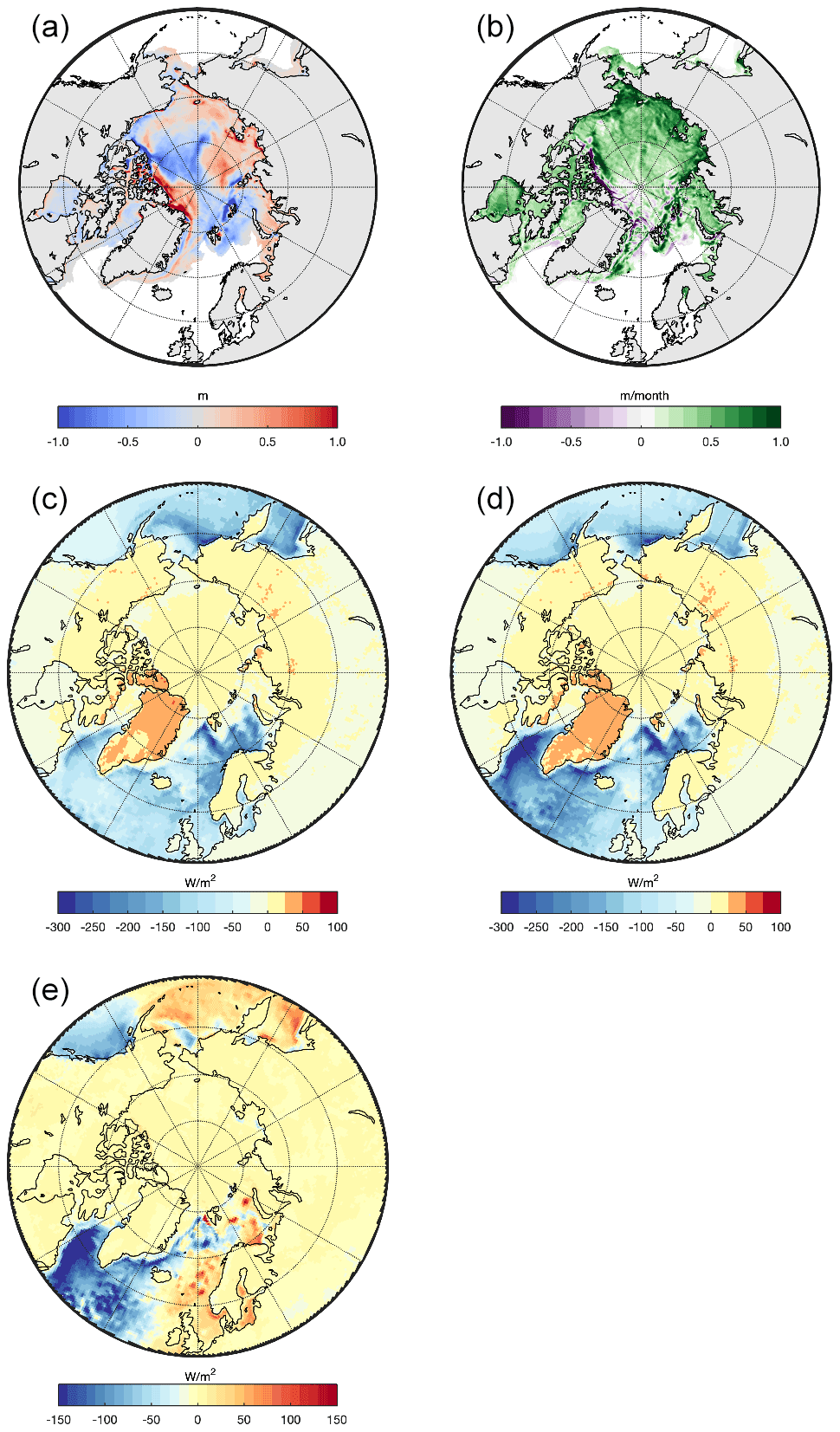
Figure 16Differences in SIT (a) and total volume tendencies (b) for JFM 2010 minus JFM 2020, mean combined sensible and latent heat fluxes (W m−2) for JFM 2010 (c) and JFM 2020 (d), and differences in surface heat fluxes for JFM2020 minus JFM 2010 (e) from the RASM hindcast simulation. Note that the flux convention means that negative fluxes are from the ocean into the atmosphere.
The SIT differences and thermodynamic ice volume differences between the JFM 2010 mean and the JFM 2020 mean were computed together with the turbulent surface heat fluxes for JFM 2010 and 2020 from the RASM hindcast simulations (Fig. 16), During the negative AO winter of 2010, the SIT was enhanced in the Beaufort and the Siberian seas and in a belt from the north coast of Greenland to the Canadian Arctic, with SIT differences of greater than 1 m. In the western part of the Arctic Ocean and the BKS, ice thickness was weaker in JFM 2010 compared to JFM 2020. The thermodynamic ice volume tendencies indicate stronger sea ice growth over most parts of the Arctic Ocean in JFM 2010 except north of Greenland and in parts of the BKS.
During winter, the surface heat budget is dominated by sensible and latent heat fluxes from the ocean to the atmosphere, which are maintained by the continuous inflow of warm Atlantic water. Compared to JFM 2010, the surface heat fluxes are stronger during the positive AO phase of winter 2020 in the North Atlantic Ocean south and east of Greenland, in the western BS region, and at the North American coast, on the Pacific side (Fig. 16). Negative values mean that the ocean is losing heat to the atmosphere. The difference plot in Fig. 16e identifies enhanced heat flux changes in the North Atlantic around and south of Greenland, along the eastern coast of Greenland, and in the western BS, with values of 150 W m−2 during the positive AO phase. The magnitude of surface heat fluxes in the BS is strongly linked to the inflow of warm Atlantic water from the Norwegian Sea (Smedsrud et al., 2013), hence enhanced surface heat fluxes during the winter of 2020 should be associated with reduced sea ice cover due to increased oceanic heat inflow. However, the BS ice extent during that winter was the largest since 2004 (https://cryo.met.no/en/sea-ice-index-bar, last access: 28 February 2022), which implies an increased and dominant role of dynamics (DVT) in the positive sea ice thickness anomalies in the region.
This difference structure on the North Atlantic side agrees very well with the NCEP-based surface heat flux analysis of Zhao et al. (2019), who showed a high correlation between the sensible heat fluxes in this North Atlantic region and the AO index (their Fig. 8a), with enhanced surface heat fluxes occurring during a more positive AO phase. The main factor mediating the turbulent surface heat fluxes is the meridional wind component in the Nordic Seas. Zhao et al. (2019) showed that when the AO index is positive, the atmospheric circulation enhances the transport of warm and humid air into the Arctic along the Norwegian coast through southerly winds as well as the transport of cold and dry air to the Atlantic along the Greenland Sea coast via northerly winds (see their Fig. 10). The view of Gong et al. (2020) (their Fig. 7f) that heating anomalies in Greenland, the BS and the Kara Sea are a possible source of planetary wave activity over the Arctic Ocean may be supported by our results (Fig. 16).
Monthly averaged sea ice thicknesses from remotely sensed data based on the ESA CryoSat-2/SMOS data set allowed the determination of Arctic-wide sea ice thickness distributions between 15 October 2019 and 15 April 2020. We analyzed and compared the satellite-derived sea ice thickness product with results from a hindcast simulation using the coupled RASM from November 2019 until March 2020.
From January to March 2020, the permanent positive AO phase was accompanied by a positive phase of the AD pattern. A comparison of the SITs for November 2019 and JFM 2020 indicated that there was thicker ice in the central Arctic in the CryoSat2/SMOS data compared to the RASM. In the BS, the Laptev Sea and the Bering Strait, RASM simulates up to 1 m thicker sea ice compared to the satellite-derived data. The ice anomalies in the BKS are due to enhanced ice growth following low-temperature anomalies and the result of intensified atmospherically driven sea ice transport and deformations. The Davies Strait, the east coast of Greenland and the BS all show thinner sea ice at the ice borders, an enhanced impact of atmospheric near-surface winds and accompanying convergence and divergence changes. Strong ice growth anomalies occurred in February 2020 in the Beaufort Sea and in March 2020 over the mid-Arctic Ocean, parts of the BS, and the east coast of Greenland. The positive sea ice thickness anomaly in the BS during January 2020 and March 2020 is a result of enhanced ice growth (related to the negative temperature anomalies in this area) and a consequence of intensified sea ice convergence and ice shear. The BS ice extent during these months was the largest since 2004, which implies an increased and dominant role of dynamics in the positive sea ice thickness anomalies in the region. Compared with the dynamic contributions, thermodynamic ice growth processes led to the greatest differences in the BKS and at the ice edge region around Spitsbergen and Greenland.
The simulated and satellite-derived sea ice velocity anomalies during January–March 2020 indicate a strong acceleration of the Transpolar Drift during the MOSAiC winter. Compared to previous years, winds tended to have anomalies toward the Fram Strait, in particular in January, February and March 2020, in line with corresponding sea-level pressure patterns.
To quantify the underlying mechanisms for the Arctic ice volume differences and different temporal evolutions, we computed the thermodynamic sea ice volume tendencies for all 30 ensemble members in the forecast mode for the pan-Arctic and BS domains. The internally generated sea ice volume differences among the 30 ensemble members for the Arctic domain are in the range of 1000 km3 and indicate strong internally generated variability due to Arctic feedbacks and remote impacts from the mid-latitudes. The integrated winter ice volume tendencies under dynamic and thermodynamic drivers are largest in the BS, and driven by thermodynamic ice-growth and ice-melt processes and the impact of dynamic surface winds on sea ice formation and deformation.
A comparison of the respective SIT distributions and turbulent heat fluxes during the positive AO phase in JFM 2020 and the negative AO phase in JFM 2010 corroborates the conclusion that winter sea ice conditions in the Arctic Ocean can be significantly altered by AO variability. During the negative AO winter of 2010, sea ice growth was enhanced in the Beaufort and Siberian seas and in a belt from the north coast of the Greenland Sea to the Canadian Arctic, with sea ice differences of greater than 1 m compared to the positive AO winter of 2020. An inverse temperature anomaly pattern occurs between the western and eastern Arctic for positive and negative AO winters. The surface heat fluxes for JFM 2010 and JFM 2020 point to much stronger heat fluxes for the positive AO winter phase of 2020 in the North Atlantic Ocean south of Greenland, whereas in the BS region and on the Pacific side, the patterns look similar. This result supports the idea of Sato et al. (2014) that sea ice changes in the BS are under the control of atmospheric circulation over the Norwegian Sea and an enhanced southerly atmospheric advection connected to the northward shift of the Gulf Stream. This interplay between external drivers and internally generated variability for variations in sea ice thickness in different years requires further in-depth investigations.
Codes or data are available from the authors by request.
The supplement related to this article is available online at: https://doi.org/10.5194/tc-16-981-2022-supplement.
KD and WM conceived the study and wrote the paper. SH, YJL, HFG, TK, CH, DH and RR undertook the data analysis and developed the methods. VB, JJC, JCK, RO, MR, AR, JS and AS contributed to the interpretation of results. All authors commented on the manuscript.
The contact author has declared that neither they nor their co-authors have any competing interests.
Publisher's note: Copernicus Publications remains neutral with regard to jurisdictional claims in published maps and institutional affiliations.
This work was carried out as part of the Multidisciplinary drifting Observatory for the Study of Arctic Climate (MOSAiC) funded by the German Ministry for Education and Research (BMBF) under grant N-2014-H-060_Dethloff.
The production of the merged CryoSat-SMOS sea ice thickness data v2.02 was funded by the ESA project SMOS & CryoSat-2 Sea Ice Data Product Processing and Dissemination Service, and data from November 2010 to April 2020 were obtained from AWI (ftp://ftp.awi.de/sea_ice/product/cryosat2_smos/v202/, last access: 3 November 2021). The ESA CryoSat-2/SMOS data set was produced and disseminated by the Alfred Wegener Institute, Helmholtz Centre for Polar and Marine Research.
The AO index computations allowed comparison with those provided by the NOAA Climate Prediction Center; https://www.cpc.ncep.noaa.gov/products/precip/CWlink/daily_ao_index/ao.shtml (last access: 10 February 2022).
The ERA5 data were provided by the European Centre for Medium-Range Weather Forecasts (ECMWF).
Sea ice thickness data used in this article were produced as part of the international Multidisciplinary drifting Observatory for the Study of the Arctic Climate (MOSAiC), with the tag MOSAiC20192020 and Project ID AWI_PS122.
Wieslaw Maslowski, Younjoo J. Lee, John J. Cassano and Jaclyn Clement Kinney acknowledge partial support for the RASM contribution from the following programs: the US Department of Energy (DOE) Regional and Global Model Analysis (RGMA), the Office of Naval Research (ONR) Arctic and Global Prediction (AGP) and National Science Foundation (NSF) Arctic System Science (ARCSS); and Robert Osinski acknowledges support from the Ministry of Science and Higher Education in Poland. The US Department of Defense (DOD) High Performance Computer Modernization Program (HPCMP) provided computer resources for RASM simulations analyzed here.
Klaus Dethloff, Dörthe Handorf and Annette Rinke acknowledge the funding by the Deutsche Forschungsgemeinschaft (DFG, German Research Foundation) of the project ArctiC Amplification: Climate Relevant Atmospheric and SurfaCe Processes, and Feedback Mechanisms (AC)3 (project number 268020496, TRR 172) within the Transregional Collaborative Research Center.
Thomas Krumpen, Dörthe Handorf and Annette Rinke acknowledge the project Quantifying Rapid Climate Change in the Arctic: regional feedbacks and large-scale impacts (QUARCCS), funded by the German and Russian Ministries of Research and Education.
The authors thank the reviewers and the editor for their careful reading of the manuscript and constructive suggestions, which helped to improve it. The authors express their thanks to Copernicus publications for careful type setting and adjustments.
The article processing charges for this open-access publication were covered by the Alfred Wegener Institute, Helmholtz Centre for Polar and Marine Research (AWI).
This paper was edited by Petra Heil and reviewed by three anonymous referees.
AARI: Russian North Polar Drifting Station Data from NSIDC, Res. Data Archive at NCAR, https://doi.org/10.5065/V47S-KW40, 1993.
Armitage, T. W. K., Bacon, S., and Kwok, R.: Arctic sea level and surface circulation response to the Arctic Oscillation, Geophys. Res. Lett., 45, 6576–6584, https://doi.org/10.1029/2018GL078386, 2018.
Barton, I., Lenn, Y.-D., and Lique, C.: Observed Atlantification of the Barents Sea causes the polar front to limit the expansion of winter Sea ice, J. Phys. Oceanogr., 45, 1849–1866, https://doi.org/10.1175/JPO-D-18-0003.1, 2018.
Belter, H. J., Krumpen, T., von Albedyll, L., Alekseeva, T. A., Birnbaum, G., Frolov, S. V., Hendricks, S., Herber, A., Polyakov, I., Raphael, I., Ricker, R., Serovetnikov, S. S., Webster, M., and Haas, C.: Interannual variability in Transpolar Drift summer sea ice thickness and potential impact of Atlantification, The Cryosphere, 15, 2575–2591, https://doi.org/10.5194/tc-15-2575-2021, 2021.
Blackport, R., Screen, J. A., van der Wiel, K., and Bintanja, A.: Minimal influence of reduced Arctic sea ice on coincident cold winters in mid-latitudes, Nat. Clim. Chang., 9, 697–704, https://doi.org/10.1038/s41558-019-0551-4, 2019.
Bushuk, M., Yang, X., Winton, M., Msadek, R., Harrison, M., Rosati, A., and Gudgel, R.: The value of sustained Ocean observations for sea ice predictions in the Barents Sea, J. Climate, 32, 7017–7035, 2019.
Cai, L., Alexeev, V. A., Walsh, J. E., and Bhatt, U. S.: Patterns, Impacts, and Future Projections of Summer Variability in the Arctic from CMIP5 Models, J. Climate, 31, 9815–9833, 2018.
Cassano, J. J., DuVivier, A., Roberts, A., Hughes, M., Seefeldt, M., Brunke, M., Craig, A., Fisel, B., Gutowski, W., Hamman, J., Higgins, M., Maslowski, W., Nijssen, B., Osinski, R., and Zeng, X.: Development of the Regional Arctic System Model (RASM): Near-Surface Atmospheric Climate Sensitivity, J. Climate, 30, 5729–5753, 2017.
CICE Consortium: CICE Documentation, 27 September 2021, internal report, https://cice-consortium-cice.readthedocs.io/_/downloads/en/master/pdf (last access: 27 September 2021), 2021.
Cohen, J., Furtado, J. C., Barlow, M. A., Alexeev, V. A., and Cherry, J. E.: Arctic warming, increasing snow cover and widespread boreal winter cooling, Env. Res. Lett., 7, 014007, https://doi.org/10.1088/1748-9326/7/1/014007, 2012.
Cohen, J., Screen, J. A., Furtado, J. C., Barlow, M., Whiileston, D., Coumou, D., Francis, J., Dethloff, K., Entekhabi, D., Overland, J., and Jones, J.: Recent Arctic amplification and extreme mid-latitude weather, Nat. Geosci., 7, 627–637, https://doi.org/10.1038/ngeo2234, 2014.
Dethloff, K., Rinke, A., Benkel, A., Koeltzow, M., Sokolova, E., Kumar Saha, S. H., Handorf, D., Dorn, D., Rockel, B., von Storch, H., Haugen, J. E., Roed, L. P., Roeckner, E., Christensen, J. H., and Stendel, M.: A dynamical link between the Arctic and the global climate system, Geophys. Res. Lett., 33, L03703, https://doi.org/10.1029/2005GL025245, 2006.
Ding, Q., Schweiger, A., L'Heureux, M., Steig, E. J., Battisti, D. S., Johnson, N. C., Blanchard-Wrigglesworth, E., Po-Chedley, S., Zhang, Q., Harnos, K., Bushuk, M., Markle, B., and Baxter, I.: Fingerprints of internal drivers of Arctic sea ice loss in observations and model simulations, Nat. Geosci., 12, 28–33, https://doi.org/10.1038/s41561-018-0256-8, 2019.
Dorn, W., Dethloff, K., Rinke, A., Frickenhaus, S., Gerdes, R., Karcher, M., and Kauker, F.: Sensitivities and uncertainties in a coupled regional atmosphere-ocean-ice model with respect to the simulation of Arctic sea ice, J. Geophys. Res., 112, D10118, https://doi.org/10.1029/2006JD007814, 2007.
Dorn, W., Dethloff, K, and Rinke, A.: Improved simulation of feedbacks between atmosphere and sea ice over the Arctic Ocean in a coupled regional climate model, Ocean Model., 29, 103–114, https://doi.org/10.1016/j.ocemod.2009.03.010, 2009.
Frolov, I. E., Gudkovich, Z. M., Radionov, V. F., Shirochkov, A. V., and Timokhov, L. A.: The Arctic Basin: Results from the Russian Drifting Stations, Praxis Publishing, Chichester, 270 pp., ISBN 9783540241423, 2005.
Gammelsrød, T., Leikvin, Ø., Lien, V., Budgell, W. P., Loeng, H., and Maslowski, W.: Mass and heat transports in the NE Barents Sea: Observations and models, J. Marine Syst., 75, 56–69, https://doi.org/10.1016/j.jmarsys.2008.07.010, 2009.
Gimbert, F., Marsan, D., Weiss, J., Jourdain, N. C., and Barnier, B.: Sea ice inertial oscillations in the Arctic Basin, The Cryosphere, 6, 1187–1201, https://doi.org/10.5194/tc-6-1187-2012, 2012.
Gong, T., Feldstein, S. B., and Lee, S.: Rossby Wave Propagation from the Arctic into the Midlatitudes: Does It Arise from In Situ Latent Heating or a Trans-Arctic Wave Train?, J. Climate, 33, 3619–3633, 2020.
Haas, C.: Evaluation of ship-based electromagnetic-inductive thickness measurements of summer sea-ice in the Bellingshausen and Amundsen Seas, Antarctica, Cold Reg. Sci. Technol., 27, 1–16, 1998.
Haas, C., Rupp, K.-H., and Uuskallio, A.: Comparison of a long track EM ice thickness profiles with ship performance data, POAC '99, Proc. 15th Int. Conf. on Port and Ocean Engineering Under Arctic Conditions, Espoo, Finland, 1999, edited by: Tuhkuri, J. and Riska, K., Helsinki Univ. Techn., Ship Lab, 1, 343–353, 1999.
Hall, A.: Projecting regional change, Science, 346, 1461–1462, 2014.
Hendricks, S. and Ricker, R.: Product User Guide & Algorithm Specification: AWI CryoSat-2 Sea Ice Thickness (version 2.3), https://epic.awi.de/id/eprint/53331/ (last access: 3 November 2021), 2020.
Hersbach, H. and Dee, D.: ERA5 reanalysis is in production, ECMWF Newsletter 147, https://www.ecmwf.int/en/newsletter/147/news/era5-reanalysis-production (last access: winter 2021/22), 2016.
Inoue, J.: Review of forecast skills for weather and sea ice in supporting Arctic navigation, Polar Sci., 27, 100523, https://doi.org/10.1016/j.polar.2020.100523, 2021.
Inoue, J., Hori, M. E., and Takaya, H.: The role of Barents Sea ice in the wintertime cyclone track and emergence of a warm-Arctic cold-Siberian anomaly, J. Climate, 25, 2561e2568, https://doi.org/10.1175/JCLI-D-11-00449.1, 2012.
Jaiser, R., Dethloff, K., Handorf, D., Rinke, A., and Cohen, J.: Impact of sea ice cover changes on the Northern Hemisphere atmospheric winter circulation, Tellus, 64, 1–11, https://doi.org/10.3402/tellusa.v64i0.11595, 2012.
Johannessen, O. M., Bengtsson, L., Miles, M. W., Kuzmina, S. I., Semenov, V. A., Alekseev, G. V., Nagurnyi, A. P., Zakharov, V. F., Bobylev, L. P., Pettersson, L. H., Hasselmann, K., and Cattle, H. P.: Arctic climate change: Observed and modelled temperature and sea ice variability, Tellus A, 56, 328–341, 2004.
Joliff, J. K., Kindle, J. C., Shulman, I., Penta, B., Friedrichs, M. A. M., Helber, R., and Arnone, R. A.: Summary diagrams for coupled hydrodynamic-ecosystem model skill assessment, J. Mar. Syst., 76, 64–82, 2009.
Jutila, A., Hendricks, S., Ricker, R., von Albedyll, L., Krumpen, T., and Haas, C.: Retrieval and parameterisation of sea-ice bulk density from airborne multi-sensor measurements, The Cryosphere, 16, 259–275, https://doi.org/10.5194/tc-16-259-2022, 2022.
Kim, B.-M., Son, S.-W., Min, S.-K., Jeong, J.-H., Kim, S.-J., Zhang, X., Shim, T., and Yoon, J.-H.: Weakening of the stratospheric polar vortex by Arctic sea-ice loss, Nat. Commun., 5, 1–8, https://doi.org/10.1038/ncomms5646, 2014.
Kolstad, E. W. and Screen, J. A.: Nonstationary relationship between autumn Arctic sea ice and the winter North Atlantic Oscillation, Geophys. Res. Lett., 46, 7583–7591, 2019.
Krumpen, T., Birrien, F., Kauker, F., Rackow, T., von Albedyll, L., Angelopoulos, M., Belter, H. J., Bessonov, V., Damm, E., Dethloff, K., Haapala, J., Haas, C., Harris, C., Hendricks, S., Hoelemann, J., Hoppmann, M., Kaleschke, L., Karcher, M., Kolabutin, N., Lei, R., Lenz, J., Morgenstern, A., Nicolaus, M., Nixdorf, U., Petrovsky, T., Rabe, B., Rabenstein, L., Rex, M., Ricker, R., Rohde, J., Shimanchuk, E., Singha, S., Smolyanitsky, V., Sokolov, V., Stanton, T., Timofeeva, A., Tsamados, M., and Watkins, D.: The MOSAiC ice floe: sediment-laden survivor from the Siberian shelf, The Cryosphere, 14, 2173–2187, https://doi.org/10.5194/tc-14-2173-2020, 2020.
Krumpen, T., von Albedyll, L., Goessling, H. F., Hendricks, S., Juhls, B., Spreen, G., Willmes, S., Belter, H. J., Dethloff, K., Haas, C., Kaleschke, L., Katlein, C., Tian-Kunze, X., Ricker, R., Rostosky, P., Rückert, J., Singha, S., and Sokolova, J.: MOSAiC drift expedition from October 2019 to July 2020: sea ice conditions from space and comparison with previous years, The Cryosphere, 15, 3897–3920, https://doi.org/10.5194/tc-15-3897-2021, 2021.
Kwok, R., Spreen, G., and Pang, S.: Arctic sea ice circulation and drift speed: Decadal trends and ocean currents, J. Geophys. Res.-Oceans, 118, 2408–2425, https://doi.org/10.1002/jgrc.20191, 2013.
Landy, J. C., Petty, A. A., Tsamados, M., and Stroeve, J. C.: Sea ice roughness overlooked as a key source of uncertainty in CryoSat-2 ice freeboard retrievals, J. Geophys. Res.-Oceans, 125, e2019JC015820, https://doi.org/10.1029/2019JC015820, 2020.
Large, W. G. and Yeager, S. G.: The global climatology of an interannually varying air–sea flux data set, Clim. Dynam., 33, 341–364, https://doi.org/10.1007/s00382-008-0441-3, 2008.
Lawrence, Z. D., Perlwitz, J., Butler, A. H., Manney, G. L., Newman, P. A., Lee, S. H., and Nash, E. R.: The remarkably strong Arctic stratospheric polar vortex of winter 2020: Links to record-breaking Arctic Oscillation and ozone loss, J. Geophys. Res., 25, 1–21, https://doi.org/10.1002/essoar.10503356.1, 2020.
Legates, D. R.: The effect of domain shapes on principal components analyses: a reply, Int. J. Climatol., 13, 219–228, 1993.
Lei, R., Heil, P., Wang, J., Zhang, Z., Li, Q., and Li, N.: Characterization of sea-ice kinematic in the Arctic outflow region using buoy data, Polar Res., 35, 22658, https://doi.org/10.3402/polar.v35.22658, 2016.
Lei, R., Gui, D., Hutchings, J. K., Wang, J., and Pang, X.: Backward and foreward drift trajectories of sea ice in the northwestern Arctic ocean in response to changing atmospheric circulation, Int. J. Climatol., 39, 4372–4391, 2019.
L'Heureux, M., Butler, A., Jha, B., Kumar, A., and Wang, W.: Unusual extremes in the negative phase of the Arctic Oscillation during 2009, Geohys. Res. Lett., 37, L10704, https://doi.org/10.1029/2010GL043338, 2010.
Liptak, J. and Strong, C.: The winter atmospheric response to sea ice anomalies in the Barents Sea, J. Climate, 27, 914–924, 2014.
Long, Z. and Perrie, W.: Changes in Ocean Temperature in the Barents Sea in the Twenty-First Century, J. Climate, 30, 5901–5921, https://doi.org/10.1175/JCLI-D-16-0415.1, 2017.
Martin, T., Tsamados, M., Schroeder, D., and Feltham, D.: The impact of variable sea ice roughness on changes in Arctic Ocean surface stress: A model study, J. Geophys. Res.-Oceans, 121, 1931–1952, https://doi.org/10.1002/2015JC011186, 2016.
Maslowski, W., Kinney, J. C., Higgins, M., and Roberts, A.: The Future of Arctic Sea Ice, Ann. Rev. Earth Plant. Sci., 40, 625–654, 2012.
McCusker, K. E., Kelly, E., Fyfe, J. C., and Sigmond, M.: Twenty-five winters of unexpected Eurasian cooling unlikely due to Arctic sea-ice loss, Nat. Geosci., 9, 838–842, https://doi.org/10.1038/ngeo2820, 2016.
Nakamura, T., Nakamura, T., Yamazaki, K., Iwamoto, K., Honda, M., Miyoshi, Y., Ogawa, Y., and Ukita, J.: A negative phase shift of the winter AO/NAO due to the recent Arctic sea-ice Reduction in late autumn, J. Geophys. Res., 120, 3209–3227, https://doi.org/10.1002/2014JD022848, 2015.
Neumann, T., Martino, T. A., Markus, T., Bae, S., Bock, M., Brenner, A., Brunt, K. M., Cavanaugh, J., Fernandes, S., Hancock, D., Harbeck, K., Lee, J., Kurtz, N., Luers, P., Luthcke, S., Magruder, L., Pennington, T., Ramos-Izquierdo, L., Rebold, T., Skoog, J., and Thomas, T.: The ice, cloud and land elevation satellite-2 mission, A global geolocated photon product, Rem. Sensing Environ., 223, 111325, https://doi.org/10.1016/j.rse.2019.111325, 2019.
Nie, J., Wang, P., Yang, W., and Tan, B.: Northern hemisphere storm tracks in strong AO anomaly winters, Atmos. Sci. Lett., 9, 153–159, https://doi.org/10.1002/asl.186, 2008.
Nie, Y., Scaife, A. A., Ren, H.-L., Comer, R. E., Andrews, M. B., Davis, P., and Martin, N.: Stratospheric initial conditions provide seasonal predictability of the North Atlantic and Arctic Oscillations, Environ. Res. Lett., 17, 034006, https://doi.org/10.1088/1748-9326/ab0385, 2019.
Onarheim, I. H., Eldevik, T., Årthun, M., Ingvaldsen, R. B., and Smedsrud, L. H.: Skillful prediction of Barents Sea ice cover, Geophys. Res. Lett., 42, 5364–5371, 2015.
Orsolini, Y., Senan, R., Balsamo, G., Doblas-Reyes, F. J., Vitart, F., Weisheimer, A., Carrasco, A., and Benestad, R. E.: Impact of snow initialization on sub-seasonal forecasts, Clim. Dynam., 41, 1969–1982, 2013.
Overland, J. E. and Wang, M.: Large-scale atmospheric circulation changes are associated with the recent loss of Arctic sea ice, Tellus, 62A, 1–9, https://doi.org/10.1111/j.1600-0870.2009.00421.x, 2010.
Peings, Y. and Magnusdottir, G.: Response of the wintertime Northern Hemisphere atmospheric circulation to current and projected Arctic sea ice decline: a numerical study with CAM5, J. Climate, 27, 244–264, 2014.
Platov, G., Iakshina, D., and Krupchatinikov, V.: Characteristics of Atmospheric Circulation Associated with Variability of Sea Ice in the Arctic, Geosciences, 10, 359, https://doi.org/10.3390/geosciences10090359, 2020.
Polarstern: Alfred-Wegener-Institut Helmholtz-Zentrum für Polar- und Meeresforschun, Polar Research and Supply Vessel POLARSTERN Operated by the Alfred-Wegener-Institute, Journal of large-scale research facilities, 3, A119, https://doi.org/10.17815/jlsrf-3-163, 2017.
Polyakov, I., Rippeth, T. P., Fer, I., Alkire, M. B., Baumann, T. M., Carmack, R. C., Ingvaldsen, R. , Ivanov, V. V., Janout, M., Lind, S., Padman, L., Pnyushkov, A. V., and Rember, R.: Weakening of Cold Halocline Layer Exposes Sea Ice to Oceanic Heat in the Eastern Arctic Ocean, J. Climate, 33, 8107–8123, https://doi.org/10.1175/JCLI-D-19-0976.1, 2020.
Proshutinsky, A., and Johnson, M.: Two circulation regimes of the wind-driven Arctic Ocean, J. Geophys. Res., 102, 12493–12514, https://doi.org/10.1029/97JC00738, 1997.
Ricker, R.: CryoSat-2/SMOS Merged Product, Description Document (PDD), Technical Report, https://earth.esa.int/eogateway/catalog/smos-cryosat-l4-sea-ice-thickness (last access: 3 November 2021), 2020.
Ricker, R., Hendricks, S., Kaleschke, L., Tian-Kunze, X., King, J., and Haas, C.: A weekly Arctic sea-ice thickness data record from merged CryoSat-2 and SMOS satellite data, The Cryosphere, 11, 1607–1623, https://doi.org/10.5194/tc-11-1607-2017, 2017.
Roberts, A. F., Hunke, E. C., Allard, R., Bailey, D. A., Craig, A. P., Lemieux, J.-F., and Turner, M. D.: Quality control for community-based sea-ice model development, Phil. Trans. R. Soc., A376, 2017.0344, https://doi.org/10.1098/rsta.2017.0344, 2018.
Sato, K., Inoue, I., and Watanabe, K.: Influence of the Gulf Stream on the Barents Sea ice retreat and Eurasian coldness during early winter, Environ. Res. Lett., 9, 08400, https://doi.org/10.1088/1748-9326/9/8/084009, 2014.
Schlichtholz, P.: Subsurface ocean flywheel of coupled climate variability in the Barents Sea hotspot of global warming, Nat. Sci. Rep., 9, 13692, https://doi.org/10.1038/s41598-019-49965-6, 2019.
Screen, J. A., Simmonds, I., Deser, C., and Tomas, R.: The Atmospheric Response to Three Decades of Observed Arctic Sea Ice Loss, J. Climate, 26, 1230–1248, 2013.
Serreze, M. C. and Stroeve, J.: Arctic sea ice trends, variability and implications for seasonal ice forecasting, Phil. Trans. R. Soc., A373, 20140159, https://doi.org/10.1098/rsta.2014.0159, 2015.
Serreze, M. C., Carse, F., Barry, R. G., and Rogers, J. C.: Icelandic Low Cyclone Activity: Climatological Features, Linkages with the NAO, and Relationships with Recent Changes in the Northern Hemisphere Circulation, J. Climate, 10, 453–464, 1997.
Smedsrud, L. H., Esau, I., Ingvaldsen, R. B., Eldevik, T., Haugan, P. M., Li, C., Lien, V. S., Olsen, A., Omar, A. M., Otterå, O. H., Risebrobakken, B., Sandø, A. B., Semenov, V. A., and Sorokina, S. A.: The role of the Barents Sea in the Arctic climate system, Rev. Geophys., 51, 415–449, https://doi.org/10.1002/rog.20017, 2013.
Sokolova, E., Dethloff, K., Rinke, A., and Benkel, A.: Planetary and synoptic scale adjustment of the Arctic atmosphere to sea ice cover changes, Geophys. Res. Lett., 34, L17816, https://doi.org/10.1029/2007GL030218, 2007.
Spreen, G., Kaleschke, L., and Heygster, G.: Sea ice remote sensing using AMSR-E 98 Ghz channels, J. Geophys. Res., 113, C02S03, https://doi.org/10.1029/2005JC003384, 2008.
Spreen, G., Kwok, R., and Menemenlis, D.: Trends in Arctic sea ice drift and role of wind forcing; 1992–2009, Geophys. Res. Lett., 38, L19501, https://doi.org/10.1029/2011GL048970, 2011.
Steele, M., Morley, R., and Ermold, W.: PHC: A Global Ocean Hydrography with a High-Quality Arctic Ocean, J. Climate, 14, 2079–2087, 2001.
Stern, H. L. and Moritz, R. E.: Sea ice kinematics and surface properties from RADARSAT synthetic aperture radar during the SHEBA drift, J. Geophys. Res.-Oceans, 107, C10, https://doi.org/10.1029/2000JC000472, 2002.
Taylor, K. E.: Summarizing multiple aspects of model performance in a single diagram, J. Geophys. Res., 106, 7183–7192, 2001.
Tian-Kunze, X., Kaleschke, L., Maaß, N., Mäkynen, M., Serra, N., Drusch, M., and Krumpen, T.: SMOS-derived thin sea ice thickness: algorithm baseline, product specifications and initial verification, The Cryosphere, 8, 997–1018, https://doi.org/10.5194/tc-8-997-2014, 2014.
Tilling, R. L., Ridout, A., and Shepherd, A.: Estimating Arctic sea ice thickness and volume using CryoSat-2 radar altimeter data, Adv. Space Res., 62, 1203–1225, 2018.
Trofimov, A., Ingvaldsen, R., and Lien, V.: Meteorological and oceanographic conditions, ICES Scient. Rep., 2, 30–46, WG on the integrated asessments of the Barents Sea, ICES. 2020, Working Group on the Integrated Assessments of the Barents Sea (WGIBAR), ICES Scientific Reports, 2, 30, 206 pp., https://doi.org/10.17895/ices.pub.5998, 2020.
Vihma, T., Tisler, P., and Uotila, P.: Atmospheric forcing on the drift of Arctic sea ice in 1989–2009, Geophys. Res. Lett., 39, L02501, https://doi.org/10.1029/2011gl050118, 2012.
Wang, Q., Danilov, S., Mu, L., Sidorenko, D., and Wekerle, C.: Lasting impact of winds on Arctic sea ice through the ocean's memory, The Cryosphere, 15, 4703–4725, https://doi.org/10.5194/tc-15-4703-2021, 2021.
Watanabe, E., Wang, J., Sumi, A., and Hasumi, H.: Arctic dipole anomaly and its contribution to sea ice export from the Arctic Ocean in the 20th century, Geophys. Res. Lett., 33, 1–4, 2006.
West, A., Blockley, E., and Collins, M.: Understanding model spread in sea ice volume by attribution of model differences in seasonal ice growth and melt, The Cryosphere Discuss. [preprint], https://doi.org/10.5194/tc-2021-351, in review, 2021.
Wu, B., Wang, J., and Walsh, J. E.: Dipole anomaly in the winter Arctic atmosphere and its association with sea ice motion, J. Climate, 19, 210–225, https://doi.org/10.1175/JCLI3619.1, 2006.
Zhang, R.: Mechanisms for low-frequency variability of summer Arctic sea ice extent, P. Natl. Acad. Sci. USA, 112, 4570–4575, https://doi.org/10.1073/pnas.1422296112, 2015.
Zhao, J., Drinkwater, K., and Wang, X.: Positive and negative feedbacks related to the Arctic Oscillation revealed by air-sea heat fluxes, Tellus, 71, 1596519, https://doi.org/10.1080/16000870.2019.1596519, 2019.
Zwally, H. J., Schutz, B., Abdalati, W., Abshire, J., Bentley, C., Brenner, A., Bufton, J., Dezio, J., Hancock, D., Harding, D., Herring, T., Minster, B., Quinn, K., Palm, S., Spinhirne, J., and Thomas, R.: ICESat's laser measurements of polar ice, atmosphere, ocean, and land, J. Geodyn., 34, 405–445, 2002.