the Creative Commons Attribution 4.0 License.
the Creative Commons Attribution 4.0 License.
 | 20 Dec 2022
Long-term firn and mass balance modelling for Abramov Glacier in the data-scarce Pamir Alay
Marlene Kronenberg
Ward van Pelt
Horst Machguth
Joel Fiddes
Martin Hoelzle
Felix Pertziger
Several studies identified heterogeneous glacier mass changes in western High Mountain Asia over the last decades. Causes for these mass change patterns are still not fully understood. Modelling the physical interactions between glacier surface and atmosphere over several decades can provide insight into relevant processes. Such model applications, however, have data needs which are usually not met in these data-scarce regions. Exceptionally detailed glaciological and meteorological data exist for the Abramov Glacier in the Pamir Alay range. In this study, we use weather station measurements in combination with downscaled reanalysis data to force a coupled surface energy balance–multilayer subsurface model for Abramov Glacier for 52 years. Available in situ data are used for model calibration and validation. We find an overall negative mass balance of −0.27 for 1968/1969–2019/2020 and a loss of firn pore space causing a reduction of internal accumulation. Despite increasing air temperatures, we do not find an acceleration of glacier-wide mass loss over time. Such an acceleration is compensated for by increasing precipitation rates (+0.0022 , significant at a 90 % confidence level). Our results indicate a significant correlation between annual mass balance and precipitation (R2 = 0.72).
- Article
(4081 KB) - Full-text XML
-
Supplement
(19358 KB) - BibTeX
- EndNote


Spatially heterogeneous mass changes of glaciers in High Mountain Asia (HMA) during the last decade have been detected by several regional studies (e.g. Kääb et al., 2012; Brun et al., 2017; Shean et al., 2020; Jakob et al., 2021). Topographical effects in combination with precipitation increases are suggested as reasons for balanced or positive mass changes for numerous glaciers in the Karakoram, Kunlun Shan, Pamir, Pamir Alay and Tibetan Plateau subregions (Miles et al., 2021). Whereas reliable precipitation data from in situ measurements are very scarce for the region (Pohl et al., 2015), the analysis of the gridded Global Precipitation Climatology Project over 30 years has indicated a precipitation increase in the western part of HMA due to large-scale atmospheric circulation patterns (strengthening westerlies) (Yao et al., 2012). Based on regional climate model data, glacier modelling and moisture tracking, De Kok et al. (2020) conclude that changes in irrigation patterns and climate are responsible for the identified mass balance patterns in HMA.
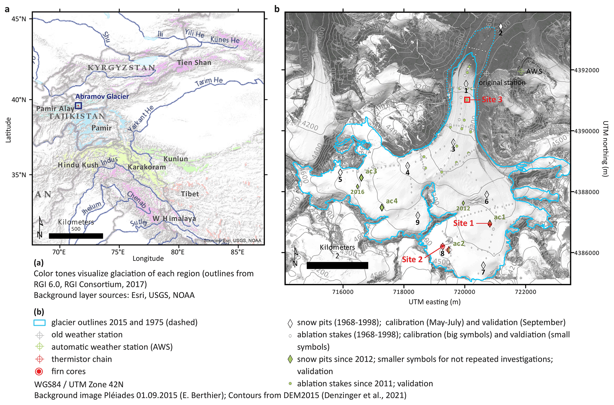
Figure 1(a) Overview map showing the location of Abramov Glacier in the Pamir Alay (indicated in blue). (b) Map of Abramov Glacier and surroundings showing the location of weather stations and the mass balance observation network (own maps; layer sources are indicated in the legend).
Including in situ data and investigating processes at a local scale over several decades can be helpful in better understanding the influence of atmospheric conditions on glacier mass changes (Mölg et al., 2012; Zhu et al., 2020). Mass balance models of varying complexity have been applied to investigate the mass balance response of mountain glaciers to climate (e.g. Klok and Oerlemans, 2002; Pellicciotti et al., 2009; Sicart et al., 2011). Models solving the energy balance at the glacier surface are more physically based and therefore considered more suitable for longer time periods with unknown climate than temperature-index parameterizations calibrated for stationary conditions (Hock, 2005). Energy balance models are, however, only applicable if sufficient data are available to generate a complete climate forcing and to calibrate uncertain model parameters. Important processes in the accumulation zone, which reduces mass loss due to refreezing and water storage, are not included into surface energy balance models. Several studies have applied energy balance models coupled to multi-layer snow models to simulate refreezing processes within the snow and firn, as well as heat conduction, which are relevant for the glacier mass and energy balance (e.g. Reijmer and Hock, 2008; Huintjes et al., 2015b). Simulating the physical connection between the atmosphere and the glacier provides insights into the climatic control of glacier mass gain or loss (Mölg and Hardy, 2004).
A few studies have applied energy balance models for glaciers in HMA: Kayastha et al. (1999) applied a point-scale energy balance model to Glacier AX010 in the Nepalese Himalaya. Azam et al. (2014) modelled the point energy balance of Chhota Shigri Glacier glacier in the Western Himalaya. Several studies focus on glaciers and ice caps located on the Tibetan Plateau (Mölg et al., 2012; Zhang et al., 2013; Huintjes et al., 2015a, b, 2016). Zhu et al. (2020) applied a surface energy balance model to Muji Glacier, located in the north-eastern Pamir. Except for Huintjes et al. (2016), who used a coupled snowpack and ice surface energy and mass balance model (COSIMA) to reconstruct the climate on the Tibetan Plateau during the little ice age, only relative short periods up to one decade have been investigated. The availability of historical data for the Abramov Glacier, located in the Pamir Alay, provides a unique opportunity for detailed modelling over longer periods than covered by those previous studies.
Abramov Glacier is located in the western part of HMA nearby to the data-scarce regions for which positive or balanced mass changes have been identified (Fig. 1). Barandun et al. (2015) previously calculated the long-term mass balance of Abramov Glacier by applying a simplified energy balance model (Oerlemans, 2001) and calibrating it to in situ measurements. Denzinger et al. (2021) computed the geodetic mass balance based on aerial imagery from 1975 and satellite stereo-pairs from 2015. Both studies found an overall negative mass balance of −0.44 ± 0.10 for 1968–2014 and of −0.38 ± 0.12 for 1975–2015. According to Barandun et al. (2021), Abramov Glacier has a similar mass balance to other glaciers in the Pamir Alay. Recent firn investigations at a point site at ∼ 4400 on Abramov Glacier (site 2 in Fig. 1b) suggest that the glacier experienced a precipitation increase compared to the 1970s and that firn conditions remained similar since then (Kronenberg et al., 2021a). These field data, however, only provide information about net accumulation rates and furthermore have a limited temporal and spatial resolution. Modelling the continuous firn and mass balance evolution of Abramov Glacier with a process-based model will allow us to put the observations into context and give insights into underlying processes. Such a model application of unprecedented detail for western HMA is possible thanks to detailed glaciological and meteorological measurements available for the temperate, valley-type Abramov Glacier (Kislov, 1982; Pertziger, 1996; Schöne et al., 2013; Hoelzle et al., 2017).
Here, we apply a coupled surface energy balance–multilayer subsurface model (van Pelt et al., 2012, 2019) to simulate the firn and mass balance evolution from 1968 to 2020. Our objective is to better understand the underlying processes of observed mass balances for this glacier in response to climatic conditions which may likely be relevant also for other sites in the region. In our analysis, we put a main focus on the accumulation area, aiming at a process-based temporally resolved quantification of accumulation processes within the firn as well as their contribution to the glacier-wide mass balance.
2.1 Study site
Abramov Glacier (39.50∘ N, 71.55∘ E) is located in the Pamir Alay (north-western Pamir) in Kyrgyzstan (Fig. 1). The north-facing valley-type glacier spans an elevation range from 3650–5000 and covers an area of 24 km2 (in 2015). In 1972/73 the glacier advanced suddenly (e.g Glazyrin et al., 1993). Since then, the glacier retreated by about 1 km (Barandun et al., 2015). The mean annual air temperature (1968–1998) measured at 3837 next to the glacier tongue (Fig. 1b, original station) was −4.1 ∘C, and annual precipitation sums for the same period are 750 mm a−1. Abramov Glacier has temperate firn conditions (Kislov, 1977), and cold subsurface conditions were measured in the ablation area throughout the year (Kislov et al., 1977). Liquid water was observed at depths of about 8.5 to 13 m around 4400 (Glazyrin et al., 1977; Kislov, 1982). The glacier's detailed and comprehensive mass-balance time series ended abruptly in 1999 but were re-initiated in 2011, and an automatic weather station (AWS) was installed in 2011 (Schöne et al., 2013; Hoelzle et al., 2017; Zech et al., 2021).
2.2 Model description
We simulate the mass balance evolution of Abramov Glacier using a coupled surface energy balance–multilayer subsurface model (EBFM) by van Pelt et al. (2012). The surface energy balance model was developed following Klok and Oerlemans (2002) and the subsurface model based on SOMARS by Greuell and Konzelmann (1994). The original model was first employed to simulate the mass balance of Nordenskiöldbreen located on Svalbard. A parameterized water percolation routine was introduced by Marchenko et al. (2017), and the albedo decay scheme was updated based on the work by Bougamont et al. (2005). The model has participated in the firn meltwater Retention Model Intercomparison Project (RetMIP) as “UppsalaUniDeepPerc” (Vandecrux et al., 2020), and it has been applied to several other glaciers located in the Arctic and the Alps (e.g. van Pelt and Kohler, 2015; van Pelt et al., 2021; Mattea et al., 2021). Here, we use the model version described by van Pelt et al. (2019), and we include an updated parametrization for seasonal snow densification after van Kampenhout et al. (2017). As the model has been previously described in detail, only a short model overview is given in the following. For full details the reader is referred to van Pelt et al. (2019) and preceding studies. The model code version used here is provided by Kronenberg et al. (2021b).
2.2.1 Surface energy balance model
The surface energy balance model is forced by meteorological input data and calculates the energy fluxes which contribute to the surface energy budget (fluxes towards the surface are defined as positive):
with the total energy available for melting Qmelt, the net short-wave radiation SWnet, the net long-wave radiation LWnet, the turbulent sensible and latent heat fluxes Qsens and Qlat, and the heat flux into the subsurface Qsub. The model iteratively solves Eq. (1) to find the surface temperature, which is the only unknown and cannot be larger than 0 ∘C.
Surface ablation occurs either in the form of melt or as sublimation when the latent heat flux is negative. Surface accumulation occurs either in the form of solid precipitation, which is calculated based on air temperature and precipitation forcing using a linear transition from rain to snow around a threshold temperature (Tsr ± 1 K), or in the form of riming. In the case of a snow or firn surface, liquid water originating from surface melt, rain or condensation is added to the subsurface (Sect. 2.2.2), and in the case of an ice surface, it leaves the system as runoff. For the entire modelling period, the incoming short-wave radiation SWin is simulated as described in Klok and Oerlemans (2002) and van Pelt et al. (2012) and accounts for grid aspect and shading by surrounding terrain. The attenuation by clouds (τcl) is calculated using Eq. (6) with parameters determined for Nordenskiöldbreen, Svalbard, by van Pelt et al. (2012). We also tested the parameter values determined by Greuell et al. (1997) for an Alpine glacier. Using the values determined for Svalbard, however, yielded a better agreement between modelled SWin and AWS measurements. The outgoing short-wave radiation SWout depends on the surface albedo. In the event that snow is present, the albedo αsnow is a function of the snow temperature, wetness and age, as described in van Pelt et al. (2019). In absence of snow, the ice albedo αice applies. The computation of the long-wave radiation follows the Stefan–Boltzmann law. The sky emissivity depends on cloud cover, air temperature and humidity following relations in Konzelmann et al. (1994) and Greuell and Konzelmann (1994).
The turbulent sensible and latent heat fluxes Qsens and Qlat are calculated for large-scale atmospheric conditions following Oerlemans and Grisogono (2002). The equations are available in Klok and Oerlemans (2002). The subsurface heat flux Qsub is calculated based on the modelled temperature and conductivity. To obtain Qsub, a linear gradient through the two uppermost layers is applied (Sect. 2.2.2). The heat supplied by liquid precipitation is neglected.
2.2.2 Subsurface model
The subsurface model computes the temporal evolution of subsurface temperature, density and liquid water content for discrete layers. The temperature depends on heat conduction (vertical diffusive heat flux) and refreezing of percolating melt, rain water and condensation of moisture (van Pelt et al., 2012). The expressions for heat capacity and effective conductivity are adopted from Sturm et al. (1997) and Yen (1981). Heat (and mass) advection is accounted for by describing vertical layer movement on a Lagrangian grid. The penetration of short-wave radiation into the subsurface and therefore also subsurface melting are neglected. We use an updated subsurface densification routine compared to previous EBFM applications. For layer densities above ρfirn = 500 kg m−3, the parametrization described in van Pelt et al. (2012), which is based on the gravitational densification by Arthern et al. (2010) and modified after Ligtenberg et al. (2011), is applied. For layers with a density below ρfirn = 500 kg m−3 a newly introduced fresh snow densification parametrization following van Kampenhout et al. (2017) is used. Seasonal snow densifies due to destructive metamorphism and compaction by overburden pressure. Van Kampenhout et al. (2017) furthermore include a snow densification due to drifting snow for densities below 350 kg m−3. Snow drift is not included here, as we are not focusing on dynamics of fresh snow. In order to increase numerical efficiency, the fresh snow ρfresh density is set to 350 kg m−3. The densification due to destructive snow metamorphism is depth independent but varies according to the layer temperature T:
with the constants cdm3 = 2.777 × 10⁻⁶ s−1, cdm4 = 0.04 K−1, and cdm2 = 1 (cdm2 = 2) in the event of absence (presence) of liquid water and a tapering constant cdm1 = 1 in the range of ρ = and exponentially decreasing above ρmax. The densification due to overburden pressure P (kg m−3) depends on a viscosity coefficient η ():
The viscosity coefficient η is calculated following van Kampenhout et al. (2017), who slightly simplified the expression of Vionnet et al. (2012):
with a correction factor accounting for the liquid water content f1, η0 = 7.62237 × 10⁶ , aη = 0.1 K−1, bη = 0.023 m3 kg−1 and cη = 358 kg m−3.
The subsurface water within the firn column originates from percolating meltwater, rain or condensed moisture. Preferential percolation is parameterized as described by Marchenko et al. (2017). Liquid water is instantly distributed along the depth axis following a normal distribution until a maximum depth zlim (see Table 2) unless it reaches an impermeable ice layer before. Refreezing of percolating water raises subsurface temperatures and densities until the melting point or the density of ice is reached. A small amount of liquid water is stored as irreducible water held by capillary forces, and the remaining water percolates further downwards until an impermeable ice layer is reached, where it forms a slush layer. The maximum irreducible water content is calculated from the porosity (ratio between pore space and the total volume of the snow/firn layer) following Schneider and Jansson (2004). Below zlim, percolation occurs non-preferentially following a bucket scheme. Water moves to the next underlying layer if the refreezing capacity is eliminated (layer density or temperature reach density of ice or melting temperature) and the maximum irreducible water content is reached. Surface runoff happens instantaneously and occurs when bare ice is at the surface.
2.3 Model setup
The surface energy balance and subsurface profiles are updated with a temporal resolution of 3 h. We use a grid of 107 × 107 grid points with a horizontal resolution of 100 m; only 2654 of these grid points are assigned to the glacier using glacier outlines from 1975. We use a digital elevation model from 1968 to define the initial elevation of each grid point and update the elevation for each 3 h time step based on a linearly downscaled annual height change grid. The topographical data were provided by Barandun et al. (2015), Denzinger et al. (2021), and Stainbank (2018). Please refer to Sect. S1.1 in the Supplement for further information on topographical data.
For each 3 h time step, we derive topographical parameters used for the computation of incoming solar radiation as described in van Pelt et al. (2012). While modelling, the glacier extent is assumed to be constant, and glacier grid points are classified as glacier throughout the modelling period. Distributed characteristics are thus computed for a fixed reference glacier surface and spatial varying elevation in time. We later account for a reduction of glacier surface when analysing the model output as described in Sect. 2.8.
The subsurface modelling domain consists of 100 vertical layers extending down to a depth of about 35 m below the surface in the accumulation area. The initial layer thickness at the surface is 0.1 m and doubles at layer numbers 15, 25 and 35 (corresponding to initial depths of 1.5, 3.5 and 7.5 m). Layer thickness reduces with time due to gravitational densification of snow and firn. The subsurface layers move along the depth axes to respond to mass gain or loss at the surface. Due to accumulation, the thickness of the uppermost layer can increase until the thickness of 0.1 m is reached; additional accumulation leads to the creation of a new layer and the removal of the lowermost layer of the modelling domain. In the EBFM, horizontal mass and energy fluxes are neglected, and mass and energy exchange between grid cells is only possible along the vertical depth axes.
2.4 Model forcing
The EBFM is forced by meteorological data with a 3-hourly resolution. The necessary input consists of the following variables: air temperature, precipitation, air pressure, relative humidity, precipitation, wind speed and cloud cover fraction. Long-term weather station measurements are available for 1968 to 1998 (Fig. 1b, original station); we extend the time series until 2020 using downscaled ERA5 reanalysis data, which are continuously available from 1979 to present (Hersbach et al., 2020).
2.4.1 Original weather station data
The original Abramov Glacier weather station was located on a moraine next to the glacier tongue at 3837 and was operational from October 1967 until summer 1999. The meteorological data were published by Pertziger (1996), who also compiled the data in digital format (daily resolution, available from Pertziger and Kronenberg, 2022). Here, we use data from January 1968 until December 1998 for the following parameters: daily average air pressure, wind speed, relative humidity, and temperature, as well as daily precipitation sum, daily minimum air temperature and cloud cover, and daily maximum temperature and cloud cover. More details about the station data can be found in Table S1 in the Supplement.
Based on these data, we created 3-hourly values for each variable. We use a scaled sine function to calculate 3-hourly air temperatures. The scaling factor is determined for each day based on measured minimum and maximum temperatures, and daily averages of the 3-hourly time series correspond to reported average air temperature measurements. For air pressure and relative humidity the mean value is applied throughout the daily cycle. Daily precipitation sums are divided by eight to obtain 3-hourly data. During the melt season, convection is a main driver of cloudiness, and cloud formation mainly takes place along the mountain ridges (Suslov and Krenke, 1980). We therefore assume cloud cover to be lower in the morning hours and lower for large areas of lower parts of the glacier than observed averages. Consequently, we assign observed daily minimum cloud cover to the first four time steps and daily average cloud cover for the rest of the day.
2.4.2 TopoSCALE ERA5 data
Long-term weather station measurements are available for 1968 to 1998 (Fig. 1b, original station); we extend the time series until 2020 using downscaled ERA5 reanalysis available from ECMWF (Hersbach et al., 2020). We use hourly output from ERA5 for 1980–2020. Data from the original Abramov weather station as well as data from the AWS are completely independent from the ERA5 data set, as the stations are not used during the assimilation procedure (Hans Hersbach, ECMWF, personal communication, 2021). We interpolate ERA5 data from the nine grid points located nearest to Abramov Glacier (Fig. S1 in the Supplement). Air temperature, air pressure, relative humidity, precipitation, and global and clear-sky radiation are downscaled using TopoSCALE (Fiddes and Gruber, 2014), which performs a 3D interpolation of atmospheric fields available on pressure levels (to account for time-varying lapse rates) and a topographic correction of radiative fluxes. The latter includes a cosine correction of incident direct short-wave radiation on a slope, an adjustment of diffuse short-wave and long-wave radiation by the sky view factor, and an elevation correction of both long-wave and direct short-wave radiation. It has been extensively tested in various geographical regions and applications, e.g. permafrost in the European Alps (Fiddes et al., 2015), permafrost in the North Atlantic region (Westermann et al., 2015), Northern Hemisphere permafrost (Obu et al., 2019), Antarctic permafrost (Obu et al., 2020), Arctic snow cover (Aalstad et al., 2018), Arctic climate change (Schuler and Østby, 2020) and Alpine snow cover (Fiddes et al., 2019). This approach enables us to provide a climate length pseudo-observation time series globally while accounting for the main topographic effects on atmospheric forcing.
2.4.3 Cloud fraction calculated from TopoSCALE ERA5 data
Cloud cover fraction is not directly available from ERA5 but a required input for the model. We therefore calculate the TopoSCALE cloud fraction from the TopoSCALE global I and the clear-sky radiation Ics. In a first step, the cloud transmissivity τcl is calculated following Klok and Oerlemans (2002):
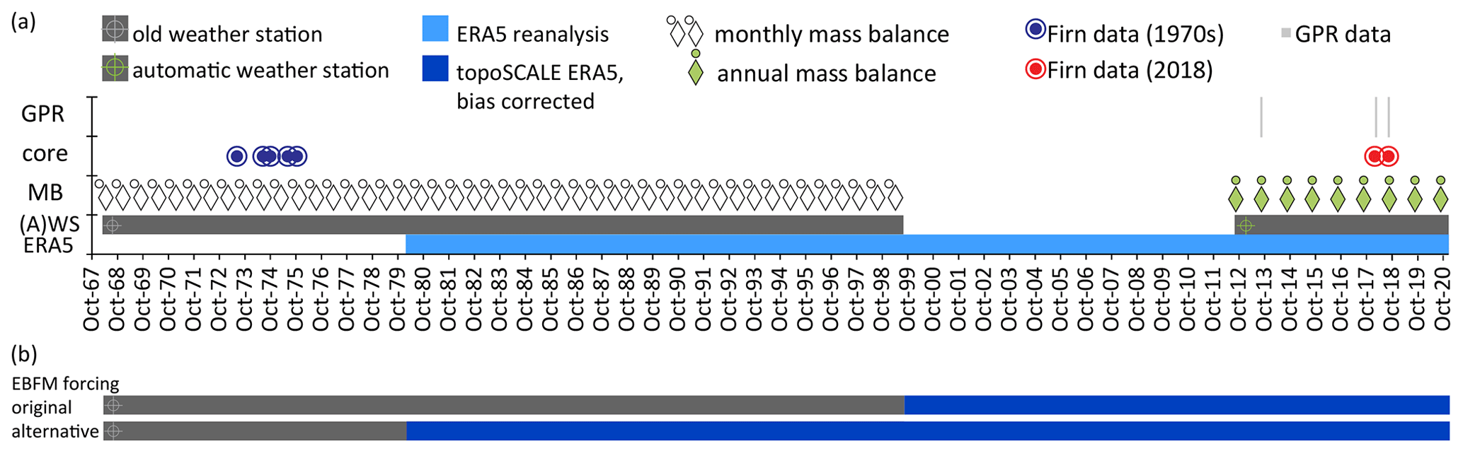
Figure 2Temporal overview of data available for this study. The availability of different in situ and gridded data sets (ERA5 reanalysis) is shown in panel (a). Panel (b) summarizes which data are used for forcing the model. We mainly show results using the original forcing. A sensitivity model run was performed using the alternative forcing (applying the same parameters as in the original run). Results are shown in the Supplement.
We use the 3-hourly average values of I and Ics to calculate τcl for each time step for which I and Icl are both above 0. We use the expression by Greuell et al. (1997),
to calculate the cloud cover n from the cloud transmissivity τcl. The parameters c1 = 0.128 and c2 = 0.346 are adopted from van Pelt et al. (2012). Night-time cloud cover n values are linearly interpolated from neighbouring, non-missing values.
2.4.4 Bias correction of TopoSCALE ERA5 data and creation of a continuous data set
ERA5 is a global reanalysis product, and its quality is dependent on the density of assimilated observations, which varies globally. Central Asia in general and mountainous regions of the Pamir specifically are data-poor, and therefore the reanalysis is less well constrained as compared to data-rich regions such as Europe. Therefore, even after downscaling (accounting for resolution differences between the model grid and point of interest), we can expect there to be residual biases, which we address with the following procedure. We aggregate TopoSCALE data to monthly averages to compare them to data from the original weather station. Biases are calculated for monthly air temperature, pressure, and wind speed for the period 1980–1998 and then used to correct TopoSCALE air temperature, pressure and wind speed for 1980–2020. Monthly average ratios between monthly aggregated station measurements and TopoSCALE data are calculated for precipitation (sums) and cloud fraction (averages) and relative humidity (averages) for the period 1980–1998 and used to correct the TopoSCALE time series for 1980–2020. The resulting cloud fraction time series for summer months (July to September) shows a reduced amplitude compared to the station time series for 1968–1998. We use the precipitation time series to correct for this by setting the cloud cover to 0 for days without precipitation and to 1 if precipitation is higher than a monthly threshold value (see Sect. S1.4 in the Supplement). Monthly averages of the final cloud fraction time series correspond to monthly averages prior to this correction. We combine the 3-hourly observed data from 1968 to 1998 with the bias-corrected TopoSCALE ERA5 data for the years 1999–2020 to obtain a final data set for 1968–2020. An alternative data set is created using historical measurements for the period 1968–1979 and TopoSCALE ERA5 data for the years 1980–2020 (Fig. 2). The data sets thus differ for the period 1980–1998. The forcing data sets are visualized in Figs. S2 and S3 in the Supplement, and the trends of original forcing are given in Table 4. Both data sets are provided by Kronenberg et al. (2021b).
2.5 Calibration and validation data
The EBFM calibration and validation is mainly based on glaciological in situ measurements which are available for two periods: historical data cover for three decades at the beginning of the simulation period (1968–1998) and in situ are again available for the most recent 8 years (2012–2020, (Fig. 2a). We split the historical data into calibration and validation data and use the recent glaciological data for validation only. Additionally, we use data from an AWS installed in 2012 to constrain parameters of the energy balance formulation (see Sect. S1.5 in the Supplement for more information).
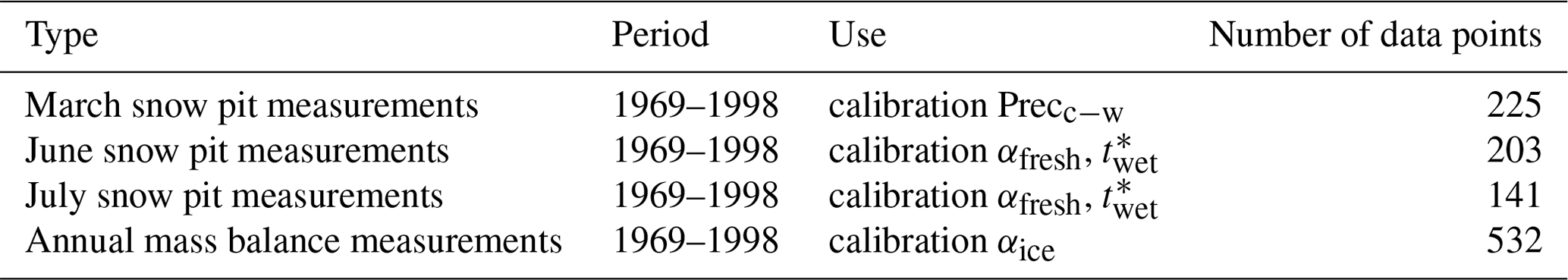
Table 1Number of point measurements used for calibration of surface energy balance parameters (see Table 2). Accumulation measurements were performed at eight sites on the glacier surface, and all available measurements are used for the selected months. We use 19 out of 165 ablation stakes for calibration. Stakes are selected to correspond to current observation sites.
2.5.1 Monthly point mass balance data 1967–1998
For Abramov Glacier, very detailed mass balance measurements are available for the period from 1967–1998 (Fig. 2). The data set consists of mass balance point observations at a monthly resolution performed at 8 snow pit and 165 stake locations totalling in 42961 stake and 2179 snow pit measurements. More details about this exceptional data set are given in Sect. S1.3 in the Supplement and provided by Pertziger and Kronenberg (2022). We use a subset of these data to calibrate several parameters of the EBFM as described in Sect. 2.6. The calibration data set consists of snow pit measurements from March, June, July, and September and measurements from 19 selected stakes locations performed at the end of the hydrological year in September (annual mass balance measurements). The stakes were selected to correspond to the location of current mass balance point observations (see Sect. 2.5.2). Up to 146 independent annual stake measurements per mass balance year are used to validate the modelled surface mass balance for the years 1968/69–1997/98. The spatial distribution of the calibration and validation data sets are shown in Fig. 1b.
2.5.2 Annual point mass balance data 2011–2020
For recent years, the modelled surface mass balances are validated against annual mass balance measurements which are available from up to 20 points since 2011/2012 (Barandun et al., 2015; Hoelzle et al., 2017; WGMS, 2022). The new monitoring network consists of 16 stakes in the ablation area and up to four snow pits in the accumulation area (Fig. 1). Whereas the stake locations were roughly kept constant over time, the locations of the snow pits varied during the first years. Field visits took place once a year during July/August, and exact observation dates are available. Only ablation stake readings from snow-free locations are considered, and the density of ice (900 kg m−3) is used to calculate floating-date mass balances between the two observation dates. Due to the stratigraphic nature of snow pit observations, the beginning of the accumulation season is not known, and we assume the last summer surface to have formed at the beginning of the hydrological year. Point accumulation values are thus calculated for the period from the 1 October until the observation date using the snow density and depth measurement of each snow pit.
2.5.3 Firn profile data
Density profiles dating back to the 1970s are available from deep firn pits that were located in the eastern branch of the accumulation area at ∼ 4400 and ∼ 4250 (Kislov, 1982). In 2018, firn cores were drilled at similar and nearby locations (Fig. 2a). We refer to Kronenberg et al. (2021a) for a detailed description of legacy and recent firn profiles. In addition to density measurements, continuous subsurface temperature measurements from four thermistors located in a borehole at ∼ 4380 are available from February 2018 until April 2020. The firn profiles and thermistor data are available from Kronenberg et al. (2022). Based on historical firn densities, one subsurface parameter was optimized (Sect. 2.6). The rest of the subsurface data are used for validation only.
2.6 Parameter selection and calibration
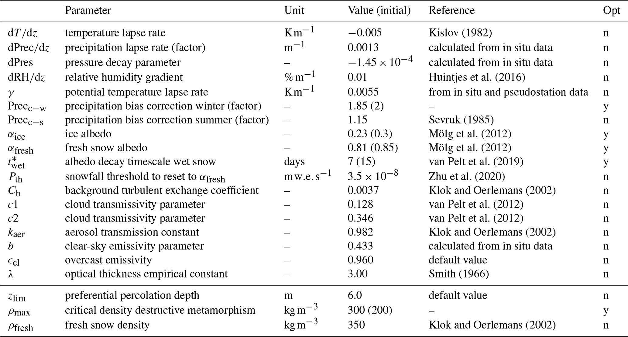
In order to reflect the local conditions of Abramov Glacier we adjusted several model parameters based on data available from in situ measurements and other studies from HMA. We selected the calibration parameters based on their relevance for our site and the existence of data. The order of calibration is chosen considering the dependence of parameters on calibration of other parameters. First, lapse rates to extrapolate the meteorological forcing over the glacier area are determined, and then the incoming radiation parameters are estimated (see Sect. S1.5 in the Supplement for details). Thereafter, we optimize accumulation parameters and finally parameters affecting summer melt. Model parameters different from values used by van Pelt et al. (2019) are summarized in Table 2; the last column indicates whether a parameter was optimized (y/n).
Kislov (1982)Huintjes et al. (2016)Sevruk (1985)Mölg et al. (2012)Mölg et al. (2012)van Pelt et al. (2019)Zhu et al. (2020)Klok and Oerlemans (2002)van Pelt et al. (2012)van Pelt et al. (2012)Klok and Oerlemans (2002)Smith (1966)Klok and Oerlemans (2002)Table 2List of EBFM parameter choices with references. For parameters optimized by EBFM simulations for Abramov Glacier (opt), the initial value is given in brackets.
We use in situ mass balance measurements from eight snow pits located on the glacier and data from a selection of 19 ablation stakes for the period 1969–1998 (Table 1) for calibration. With these data we manually optimize a set of accumulation and ablation parameters. Final parameters are determined by minimizing bias between modelled surface mass balances for grid cells corresponding to point locations with in situ measurements. We use precipitation correction factors in order to debias the precipitation forcing. The correction mainly compensates for undercatch but also accounts for all other biases present in the precipitation forcing. We consider March accumulation measurements to be least affected by melt and use them to calibrate the precipitation bias correction factor Precc−w applied for October–June. During summer months, the precipitation undercatch is assumed to be reduced compared to autumn, winter, and spring, and we adopt a value of Precc−s = 1.15 determined for Alpine locations in Switzerland from Sevruk (1985). The bias between modelled and measured June and July snow pit measurements is reduced by a two-parameter exploration for αfresh and . And finally, αice is optimized using September surface mass balance measurements (snow pits and ablation stakes).
Parameters in the subsurface model are default values except for the critical density of destructive metamorphism ρmax, which is optimized to obtain a better fit between modelled and measured subsurface densities at ∼ 4410
The comparison of optimized model simulations to surface mass balance observations used for model calibration shows a higher root mean square error (RMSE) for the annual mass balance than for the accumulation in March, and despite some bias in the linear fit, the data sets generally approach the 1:1 linear fit line (Fig. S4 in the Supplement).
2.7 Model initialization, performed simulations and sensitivity experiments
To initialize subsurface conditions the model is run twice over the period 1968–1998 using the 3-hourly weather station data to force the model. The first iteration is started with identical subsurface conditions throughout the glacier with a vertical grid consisting of temperate ice (273.15 K). The second initialization run is started from the final stage of a first run.
We perform several model runs for selected grid points corresponding to the locations of selected ablation stakes and snow pits indicated in Fig. 1 to adjust model parameters (Sect. 2.6) using the final combined 3-hourly forcing consisting of station (1968–1998) and bias-corrected TopoSCALE ERA5 data (1999–2020). Thereafter, we perform a final distributed model run for the period from 1 January 1968 until 31 December 2020 using the same forcing.
To assess the model sensitivity towards parameter choices, we performed several model runs for three selected grid points (sites 1, 2, and 3, Fig. 1b) testing single-parameter perturbations following Klok and Oerlemans (2002). Additional sensitivity runs are performed using different cloud cover forcings. To assess the overall sensitivity to the model forcing, we carried out an alternative distributed run using the alternative data set with a shorter period of station measurements (1968–1979, Fig. 2). Detailed results of these sensitivity experiments are presented in Figs. S7–S15 in the Supplement, and the code and data set used for the sensitivity experiments are provided by Kronenberg (2022).
2.8 Analysis of model output and mass balance calculation
We calculate the climatic mass balance as the sum of the surface and the internal mass balance for hydrological years (1 October–30 September) (Cogley et al., 2011). The surface mass balance is the result of accumulation (+) and ablation (−) at the surface including precipitation (+), moisture exchange (+/−), and mass loss through runoff (−). The internal mass balance accounts for refreezing and storage of liquid water below the previous summer surface.
While the model grid elevation is updated for each time step, the modelling extent is kept constant using the glacier mask from 1975 for the entire simulation period. After modelling, the glacier-wide mass balance and other variables are calculated for decade-wise updated glacier extents. Until the end of the hydrological year 1978, the entire model output is analysed. For the next 10 hydrological years, a glacier mask corresponding to the glacier area from 1986 is used, and output outside this domain is not considered. Masks based on outlines from 1998, 2005 and 2015 are used for 1988/1989–1997/1998, 1998/1999–2007/2008 and 2008/2009–2019/2020.
The equilibrium line altitude (ELA) is calculated as the mean elevation of grid points with a mass balance equal to 0 at the end of a the hydrological year. Grid points with a negative mass balance value at the end of the hydrological year are used to calculate ablation gradients, which is the linear relation between elevation and modelled ablation.
For comparison to in situ point measurements, the modelled surface mass balance of the grid point nearest to the stake/snow pit location is used. The daily model output is aggregated at the end of the month of interest with respect to the beginning of the hydrological year (1 October) to compare to accumulation observations. For comparison to ablation observations, data are accumulated until the reported observation date (Sect. 2.5.1). For in situ observations since 2011, the stake installation dates are earlier in the melt season, and model output is extracted for exact periods between stake installation and stake reading (Sect. 2.5.2).
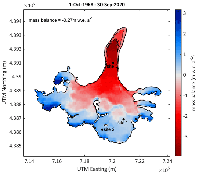
Figure 3Modelled mean annual distributed mass balance for updated glacier extents for the period from 1 October 1968 to 30 September 2020. Note that the mean annual mass balance for the entire period and updated glacier surfaces is shown. Values are thus reduced on the glacier tongue, where the glacier area is reduced over time. The different glacier outlines are shown with black lines. Furthermore, the location of three selected points is indicated.
Table 3Mean glacier-wide climatic mass balance, internal accumulation equilibrium line altitude (ELA), and ablation gradients for each decade and different periods used for comparison with other studies. The periods are hydrological years (e.g. 1968/1969–1977/1978 refers to 1 October 1968–30 September 1978) unless precise dates are specified. The mean glacier surface used for the mass balance calculation is also indicated.

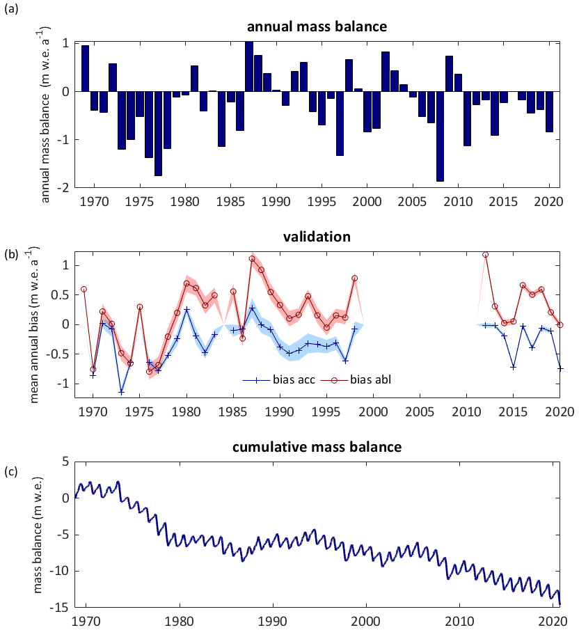
Figure 4Temporal evolution of modelled climatic mass balance. (a) Modelled mean annual mass balance for updated glacier extents. (b) Mean annual surface accumulation bias (blue) and mean annual surface ablation bias (red) between point measurements and model output for corresponding grid points. The shaded area refers to the measurement uncertainty calculated following Thibert et al. (2008). (c) Modelled cumulative mass balance for updated glacier extents.
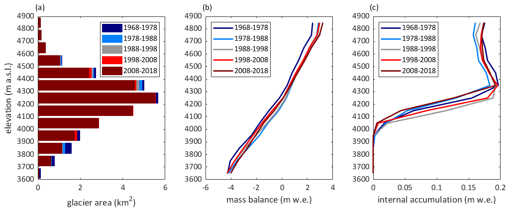
Figure 5Modelled mass balance and internal accumulation versus elevation. The elevation distribution of the glacier area for different glacier extents is shown in panel (a). The largest glacier area was observed for the first decade (shown in dark blue) and reduced over time. In panel (b) the climatic mass balance is plotted versus the elevation for the modelled decades. In panel (c) the internal accumulation is plotted versus elevation. The periods are hydrological years (e.g. 1968–1978 refers to 1 October 1968–30 September 1978).
3.1 Long-term mass balance
The distributed mean annual climatic mass balance for 1968/1969–2019/2020 is shown in Fig. 3. The mass balance of Abramov Glacier is predominantly negative for the years from 1968/1969 to 2019/2020, with a mean value of −0.27 , and shows no significant trend in annual mass balances (+0.0002 , p value = 0.979 and Fig. 4c). The most negative modelled mass balances occur at the start of the period, while the two decades between 1978 and 1998 are characterized by an almost balanced mass budget, thereafter becoming more negative again (Fig. 4a and c and Table 3). The modelled elevation distribution of mass balance shows that accumulation is lowest during the first decade (1968/1969–1977/1978) and highest during the last modelled decade (2008/2009–2017/2018), and ablation is largest during the first decade, followed by the second last decade (1998/1999–2007/2008) (Fig. 5b).
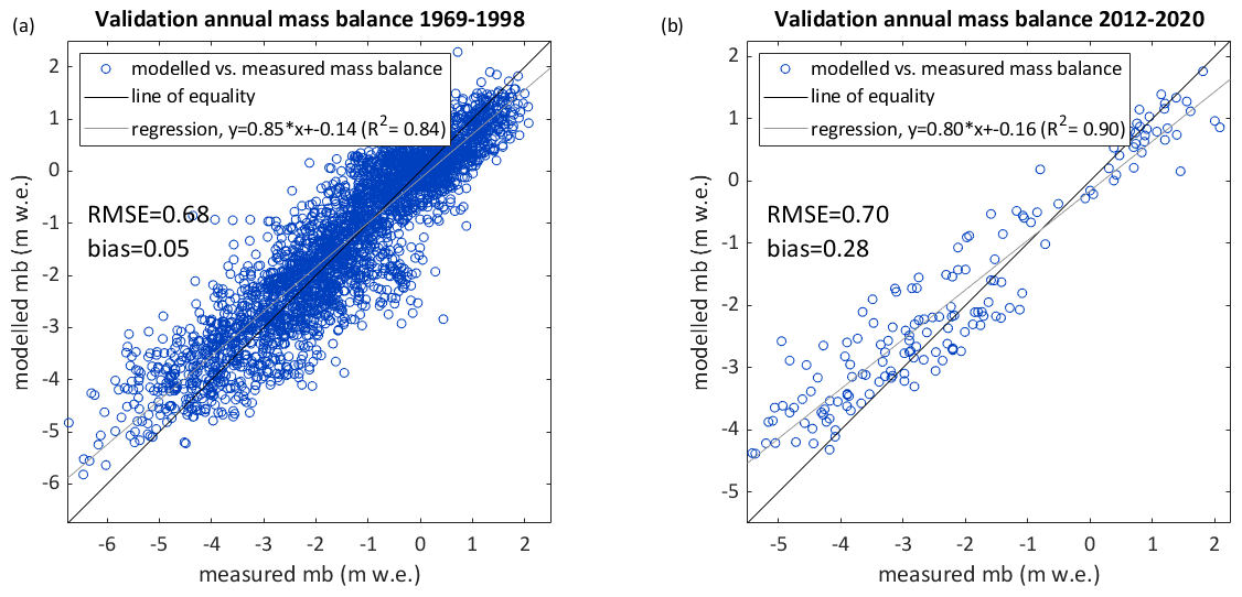
Figure 6Model validation: measured versus modelled annual surface mass balance (mb) for an independent set of point measurements from 1968/1969–1997/1998 (3292 point measurements) (a) and from 2011/2012–2019/2020 (164 point measurements) (b).
The RMSE between simulated surface mass balances and independent point measurements not used for calibration is similar for the recent and historical investigation periods (∼ 0.7 ), whereas the mean bias is lower for the period of historical measurements (+0.05 ) than for recent years (+0.28 ) (Fig. 6a and b). Differences in the mean bias are partly related to the spatial distribution of the validation data. As visible from Fig. 6a and b and Fig. 4b, both accumulation and ablation were underestimated, whereas more accumulation measurements are available for the historical period (Fig. 1b).
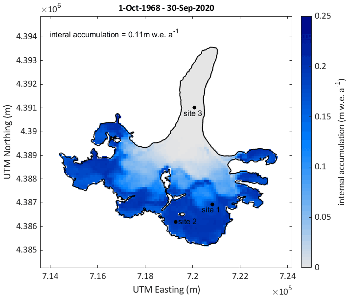
Figure 7Map of mean annual internal accumulation for the mass balance years 1968/1969–2019/2020. The location of three selected points is indicated.
3.2 Internal accumulation
The average glacier-wide modelled internal accumulation is 0.11 . Internal accumulation occurs in large parts of the accumulation area and is more pronounced in the orographic right of the accumulation area (Fig. 7) and varies over time. The highest internal accumulation rates are modelled for the years 1968/1969–1977/1978 between 4400 and 4500 (Fig. 5c). The decades 1988/1989–1997/1998 and 1998/1999–2007/2008 are characterized by higher internal accumulation rates at lower elevations around 4250 (Fig. 5b), where the glacier covers large areas (Fig. 5c). The lowest internal accumulation rates are modelled for the second and the last decade (Table 3).
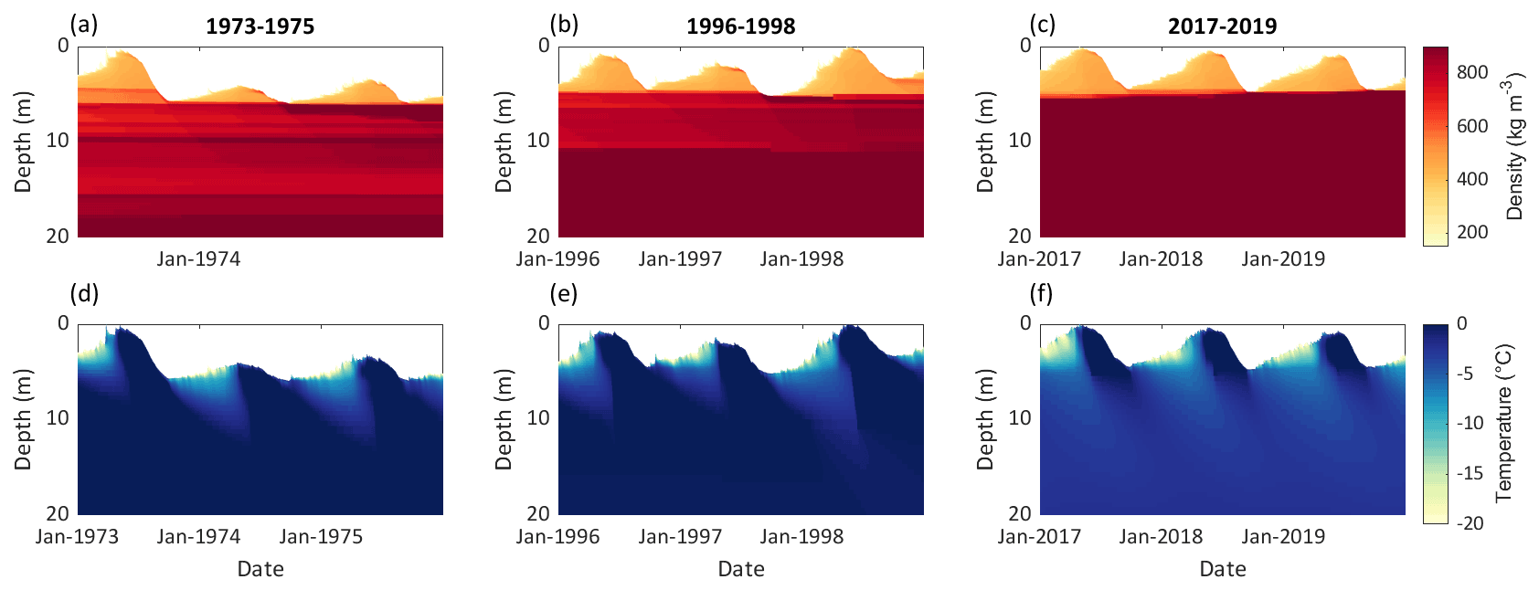
Figure 8Modelled subsurface conditions at site 1 (∼ 4250 ) for three selected periods: 1973–1975 (a, d), 1996–1998 (b, e) and 2017–2019 (c, f). Panels (a)–(c) show the subsurface density, and panels (d)–(f) show the subsurface temperature. The location of the site is indicated in Fig.1b.
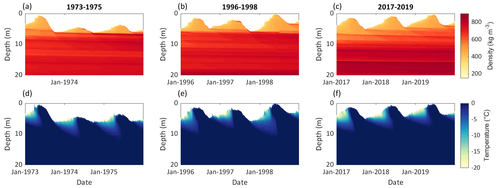
Figure 9Modelled subsurface conditions at site 2 (∼ 4400 ) for three selected periods: 1973–1975 (a, d), 1996–1998 (b, e) and 2017–2019 (c, f). Panels (a)–(c) show the subsurface density, and panels (d)–(f) show the subsurface temperature. The location of the site is indicated in Fig.1b
3.3 Firn evolution
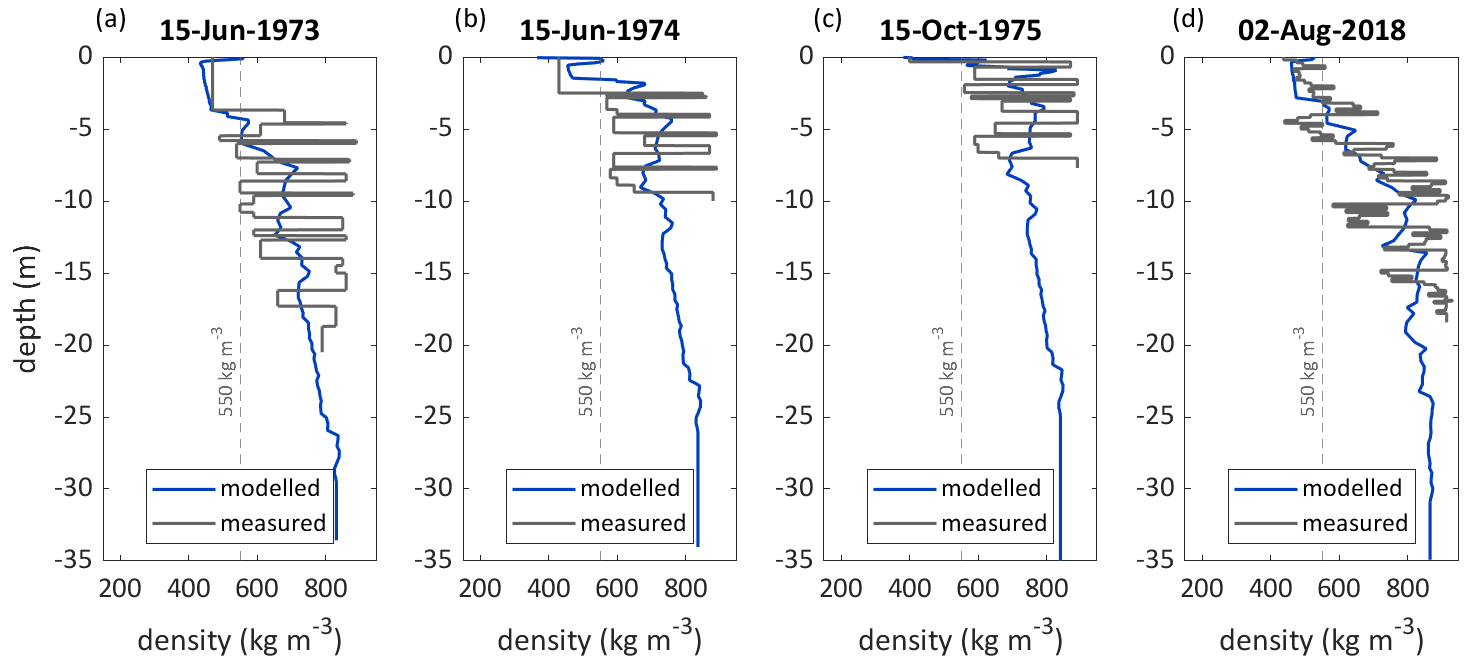
Modelled subsurface densities are higher at site 1, ∼ 4250 (Fig. 8a–c) than at site 2, ∼ 4400 (Fig. 9a–c) and increase over time at both sites. At site 1, a significant increasing trend of subsurface densities for the depth range of 0–10 m is found for 1968/1969–2019/2020 (+1.14 , p value = 0.014), whereas the trend is significant at site 2 when the first two decades are excluded (+1.53 , p value = 0.005 for 1988/1989–2019/2020). At the lower site (∼ 4250 , Fig. 8a–c) densities at depth reach the density of ice. Modelled firn densities correspond well with measurements shown for four different dates in Fig. 10. The mean biases between modelled and measured densities for the depth covered by measurements are −18.9 kg m−3 for June 1973, +52.6 kg m−3 for June 1974, +20.4 kg m−3 for June 1975 and −23.8 kg m−3 for August 2018.
For early years, the modelled subsurface temperatures indicate temperate firn conditions and propagation of winter cooling down to depths of about 10 m in the accumulation area at site 1 (∼ 4250 , Fig. 8d). In later years, the cold content propagates to greater depths, and overall cold subsurface conditions are modelled for most recent years (Fig. 8e and f). For the depth range of 0–10 m, the subsurface cooling trend is −0.036 K a−1 (p value < 0.001 for 1968/1969–2019/2020).
In contrast to the results at site 1, the modelled firn temperatures for site 2 (∼ 4400 ) indicate continuously temperate firn conditions and propagation of winter cooling down to depths of about 10 m (Fig. 9d–f). Also here, a slight cooling trend was found (−0.0041 K a−1 p value = 0.043 for 1968/1969–2019/2020).
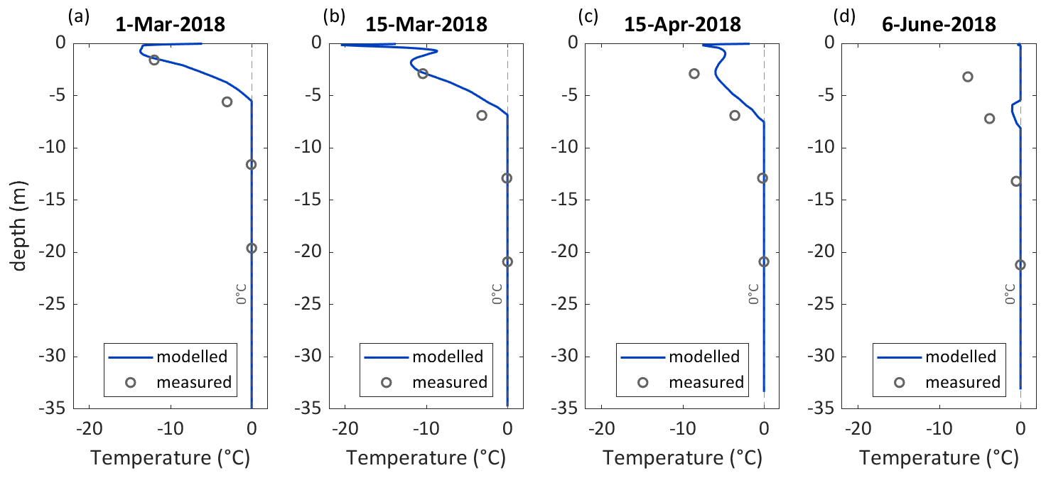
Figure 11Modelled and measured subsurface temperature for a station located near site 2 (∼ 4400 ) for four selected dates visualizing the constantly temperate conditions at depths below ∼ 10 m in spring 2018. The data are plotted for days around the onset of modelled surface melt occurring in March 2018 (a, b) and subsequent subsurface warming (b–d). The 6 June visualized in panel (d) corresponds to the date with the coldest measured temperatures at a depth of about 7 m in 2018. The location of the site is indicated in Fig. 1b.
In Fig. 11, modelled firn temperatures at site 2 are compared to thermistor measurements from spring 2018. Measured and modelled temperatures remain temperate at depths greater than about 10 m. In March (Fig. 11a and b), modelled temperatures near the surface correspond well with observations. At a depth of about 7 m, the modelled temperatures are a bit higher. In April (shown in Fig. 11c), modelled firn temperatures are warmer than measurements also for the uppermost thermistor location. At a depth of about 7 m minimum subsurface temperatures are recorded for 6 June 2018. On this date, modelled firn temperatures are temperate except for a small zone around 7 m depth (Fig. 11d).
Table 4Trends and p values for climate variables and energy balance components for the period from 1 October 1968 until 30 September 2020 (hydrological years) are listed for a grid point in the ablation area at ∼ 3850 . Values in brackets refer to site 2, located in the accumulation area at ∼ 4400 . “y” or “n” stands for significant or not significant at a 90 % confidence level. The point location of both grid points are indicated in Fig. 1. The trends for glacier-wide mass balance, glacier-wide internal accumulation and original climate forcing (for the elevation of the weather station at 3837 ; 1 October 1968–30 September 2020) are also given.

3.4 Temporal variation of climate variables, mass and energy fluxes
Significant increasing trends for model forcing air temperature (mean over hydrological years) and mean summer air temperatures are found for 1968/1969–2019/2020 (Table 4). Trends are also significant for air pressure (increase), relative humidity (decrease), cloud cover fraction (decrease) and precipitation sums (increase) (Table 4). The highest amounts of precipitation were recorded from 1978/1979 to 1997/1998 and from 2008/2009 to 2017/2018 (Table S2 in the Supplement). Whereas the earlier two decades are characterized by almost balanced mass changes, more negative values were simulated for the most recent decade, when the internal accumulation was strongly reduced compared to earlier years (Table 3). Low internal accumulation was also simulated for the second and most balanced decade (1978/1979 to 1987/1988) (Table 3). Both decades of low internal accumulation follow years with exceptionally high amounts of available melt energy and comparably low precipitation rates, especially from 1968/1969 to 1977/1978 (Tables 3 and S2; Figs. 12 and S5 in the Supplement). Overall, the preceding conditions led to a reduction of the area where internal accumulation could take place (only higher elevation bands in Fig. 5c; see also the video in the Supplement). Following 1978/1979–1987/1988, when precipitation was high, the area where internal accumulation takes place becomes larger again (Fig. 5c and video in the Supplement). In most recent years, which follow another decade characterized by negative mass balances, the area and amount of internal accumulation are strongly reduced (Table 3, Fig. 5). In general, the simulated annual mass balances are more strongly correlated with annual precipitation (R2 = 0.72) than with the summer air temperatures (R2 = 0.29, Fig. S6 in the Supplement).
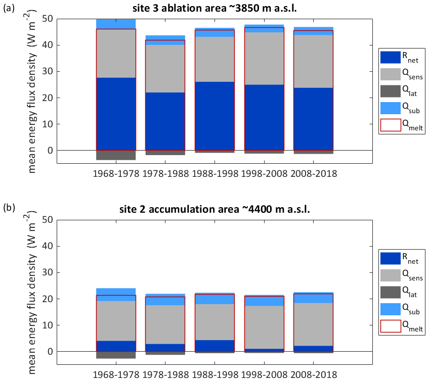
Figure 12Mean modelled energy fluxes per decade for a grid point located in the ablation area at ∼ 3850 (a) and in the accumulation area at ∼ 4400 (b). The point locations are indicated in Fig. 1. Rnet is the net radiation, Qsens the sensible heat flux and Qlat the latent heat flux, Qlat the heat flux from/into the subsurface, and Qmelt the total energy available for melt. The periods are hydrological years (e.g. 1968–1978 refers to 1 October 1968–30 September 1978).
Examining the modelled energy fluxes for different sampled locations (lower accumulation area site 1, accumulation area site 2 and ablation area site 3; Fig. 1b) highlights that most heat fluxes are characterized by an increasing trend (Table 4), whereas high incoming short-wave radiation occurred during the first decade characterized by the most pronounced mass loss (Figs. 12 and S5). In 2008/2009–2017/2018, when melt rates were highest for the points in the accumulation area, sensible heat flux and incoming long-wave radiation were high (Figs. 12 and S5, Table S2).
4.1 Long-term mass balance and firn evolution
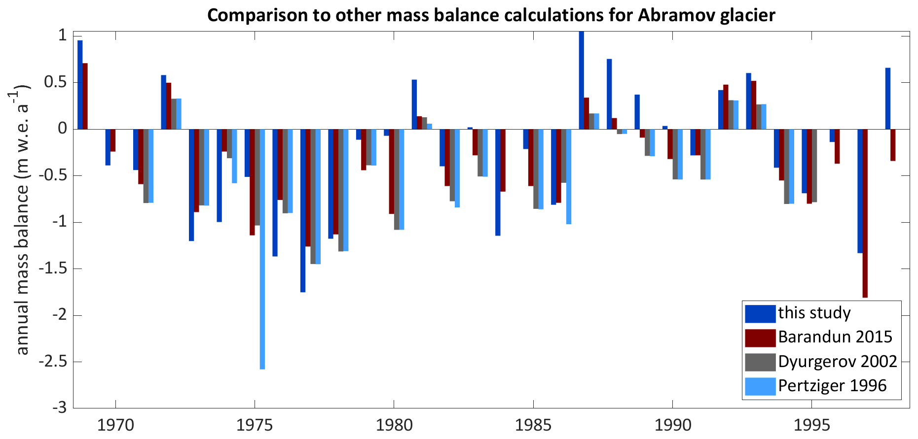
The modelled long-term mean mass balance for Abramov Glacier indicates an overall mass loss of −0.27 for the period 1968/1969–2019/2020, which is in agreement with the findings of other recent studies. Barandun et al. (2015) and Denzinger et al. (2021) found somewhat more negative mass balances. Barandun et al. (2015) estimate the mass balance for 1967/1968–2013/2014 as −0.44 ± 0.10 . Their estimate is based on the application of a calibrated surface mass balance model and a simple approximation of internal accumulation as well as basal ablation which together contribute +0.07 . In Fig. 13 annual mass balances of different studies are compared to our results: previous analysis of annual mass balance data for 1971–1994 provided different estimates but yielded all more negative mass changes (Barandun et al., 2015: −0.39 ; Dyurgerov, 2002: −0.50 ; and Pertziger, 1996: −0.61 ) than the EBFM (−0.26 ). Denzinger et al. (2021) calculate the geodetic mass balance as −0.38 ± 0.12 for 15 July 1975 until 1 September 2015. Our result for the same time period (−0.30 ) is within their calculated uncertainties.
We do not find a significant trend in the evolution of annual mass balances (+0.0002 , p value = 0.979) or in the reduction of mean annual internal accumulation (−0.0003 , p value = 0.159) for the period 1968/1969–2019/2020 despite significant trends within all variables used as model forcing (Table 4). Comparing annual mass balances with annual precipitation sums and summer air temperatures shows that annual mass balances are more strongly correlated to precipitation sums than to summer air temperatures (Fig. S6). The effect of the substantial warming (+0.0222 K a−1, p value < 0.001) thus seems to be attenuated by increasing precipitation (+0.0022 , p value = 0.074). The increase in net accumulation in the accumulation area (Fig. 5b) may thus be attributed to an increase in solid precipitation (Tables S2 and 4). Barandun et al. (2015) also find an increase in accumulation based on their modelling results as does the field study of Kronenberg et al. (2021a), who identified a net accumulation increase for a point location at ∼ 4400 We can speculate that Abramov Glacier might be affected by the same changes in precipitation patterns that could be partly responsible for the mass balance anomaly in western HMA (e.g. Miles et al., 2021). Barandun et al. (2015) furthermore describe a tendency towards more ablation during recent decades. We find high ablation rates for the first decade and for 1998/1999–2007/2008 (Fig. 5b). In contrast to previous studies (e.g. Dyurgerov and Dwyer, 2001), we do not find a steepening of ablation gradients. The ablation gradient is higher for 1968/1969–1997/1998 (0.0080 ) than for 1998/1999–2019/2020 (0.0070 ). Miles et al. (2021) calculate an ablation gradient of 0.0084 for 2012–2016. Whereas their ablation gradient is higher, their ELA of 4163 is located lower than the here modelled ELA (Table 3).
We find a relevant contribution of refreezing below the last summer horizon to the overall mass balance, and this contribution evolves over time (Fig. 5c and Table 3). In the lower accumulation area up to ∼ 4300 , internal accumulation strongly increases with elevation, and the lowest values are modelled for the last decade (Fig. 5c). At site 1, within this zone, the subsurface density reaches the density of ice (Fig. 8a–c), which will hinder subsequent internal accumulation. An increase in subsurface densities also occurs higher up in the accumulation zone at site 2 around ∼ 4400 as shown in Fig. 9a–c. The lowest internal accumulation rates are found for the second (1978/1979–1987/1988) and the last (2008/2009–2017/2018) modelled decade. Both of these periods follow decades with clearly negative mass balances and high refreezing rates (Table 3). This is confirmed by in situ measurements from several years during the first decade which indicate negative annual mass balances at several or all point observation sites in the accumulation area (Kislov, 1982; Pertziger, 1996). The model results suggest that, thanks to high accumulation and limited ablation, the firn could recover during the following years, allowing for higher internal accumulation rates thereafter. Results from the most recent decade and years, however, indicate that the necessary pore space for refreezing is again reducing. Whereas the subsurface density at ∼ 4250 decreases throughout the modelling period, a significant decrease is found for ∼ 4400 after 1987/1988 only.
Abramov Glacier is thus losing its capacity to buffer mass loss through refreezing. The loss of pore space occurs despite high amounts of solid precipitation (Table S2) responsible for the increased accumulation compared to the first decade (Fig. 5b) and affects large areas of the accumulation zone (Fig. 5a). For the upper elevation bands, modelled internal accumulation remains high for recent decades. Based on the observations from the lower firn sites, with further warming, these uppermost zones are, however, expected to also lose pore space. The changes are also reflected in a decrease in subsurface temperatures. The reduction and later absence of latent heat release through refreezing leads to cold firn properties at ∼ 4250 for recent years (Fig. 8d–f). The slight cooling trend for ∼ 4400 (Fig. 9d–f), together with the recent increase in subsurface densities, highlights that firn zone changes start to occur also at higher elevations.
Firn changes and effects on internal accumulation as identified for Abramov Glacier likely also occur elsewhere in HMA. The impacts may be delayed for glaciers with higher located elevation areas, where firn conditions may still be cold and refreezing limited. The recent propagation of changes to higher elevation ranges indicates that also higher located glaciers may experience firn regime changes in future, ultimately leading to a reduction of their firn area.
Mass balance observations often neglect internal accumulation or account for the process only in a simplified manner. This applies for mass balance calculation based on glaciological data but also for geodetic mass change estimates. The latter usually use constant density conversion factors to convert elevation to mass changes. Our results indicate that internal accumulation can play an important role for glaciers with temperate accumulation areas. Whereas mass change calculations neglecting the internal accumulation may be overestimating the mass loss for periods with available pore space, this error will likely be reduced as glaciers lose pore space.
Evidence from in situ measurements of pore space amount and change in glaciers of HMA is very scarce. Lambrecht et al. (2020) expect a strong elevation gradient of meltwater refreezing on Fedchenko Glacier, western Pamir. The chemical signature of annual accumulation layers is currently only preserved at elevations above 5200 , but evidence of summer melt was found at elevations of more than 5300 Based on sensitivity experiments with a region-wide application of a simple model, Wang et al. (2019) concluded that under warmer conditions, refreezing will increase for continental glaciers and decrease for glaciers located in more humid and warmer environments. In their study, Abramov Glacier is located in a region for which they find an increase in refreezing. Our results indicate a decrease in internal accumulation related to the retreat of the firn line. A retreat of the firn line is likely also occurring elsewhere; however, the underlying processes are often not sufficiently included into simple, regional approaches.
4.2 Uncertainties, model sensitivities and validation
EBFM reproduces the observations satisfactorily, as shown by the comparison of modelled and measured surface mass balances (Fig. 6) and the comparison of subsurface properties (Figs. 10 and 11). Whereas the overall biases between modelled and measured surface mass balances are low (0.05 for historical and 0.28 for recent years), relatively large biases exist for single years (Fig. 4b). These comparisons of modelled and measured data provide an overall estimate of the combined modelling and observational uncertainty. The sources of the modelling uncertainty are diverse and sometimes not readily quantifiable; we here discuss the general sources and likely implications based on the performed sensitivity experiments and general considerations, rather than producing a formal uncertainty assessment for the model output.
Several uncertainties are related to the model setup. The spatial vertical and horizontal as well as temporal resolutions are too coarse to resolve all the observed variations and to reproduce all relevant processes. Consequences of the horizontal resolutions are, for example, that several point observations shown in Figs. S4 and 6 are located within one modelled grid cell. The model is unable to fully reproduce the spatial heterogeneity of in situ observations. This also applies for subsurface conditions. On Abramov Glacier, highly variable firn conditions and accumulation rates are found based on firn cores and ground-penetrating radar data (Kronenberg et al., 2021a). This study showed that annual accumulation, measured in firn cores, can vary by a factor of 1.5 over a horizontal distance of 250 m. Thus the EBFM satisfyingly reproduces the bulk densities measured at site 2 (Fig. 10); however, the lower measured densities at nearby drill sites (c4381 and c4382 in Kronenberg et al., 2021a) are not reproduced satisfactorily as the model does not simulate the horizontal small-scale variability of accumulation and furthermore does not consider processes such as wind redistribution of snow. The lack of considering those processes also explains the misfit between modelled and measured accumulation as visible from Fig. 6a and b and Fig. S4a and b to some extent. Other reasons for the misfit are likely related to the limited spatial representativeness of the rather low number of accumulation observations. Another uncertainty related to the model setup is the use of a linearly updated glacier surface elevations and decade-wise changing glacier outlines. These approximations of topographical changes may be responsible for underestimations (overestimations) of melt rates on the glacier tongue if surface elevations are too high (too low). The linearly updated glacier surface might thus be a reason for the underestimation of melt rates on the glacier tongue as visible from Fig. 6a and b and Fig. S4b. The initial conditions are a further source of uncertainties. It is very likely that the atmospheric conditions were different from the used data set prior to the modelling period. Nevertheless, modelled subsurface conditions agree well with measurements during early years of the modelling period (Fig. 10a–c).
An important source of uncertainties is related to the model forcing. While station data are available for the first 30 years, data from a gridded climate product (ERA5) have to be used for the remaining modelling period. To homogenize the input, the downscaled ERA5 data are bias corrected to match with monthly averages of observations for the overlapping period. The creation of a cloud cover forcing is needed for additional processing steps. Furthermore, the cloud cover forcing from the period with measurements is another source of uncertainties which are related to the observational nature of the data and our choice to implement sub-daily cloud cover variations throughout the year while keeping precipitation constant throughout a day. The sensitivity of cloud cover related choices is shown in Figs. S9 and S10 in the Supplement. Despite the corrections of the TopoSCALE ERA5 forcing, differences in both data sets affect the model output as evident from the results of the alternative model run which yielded a more negative mass balance for the period for which both data sets are available (alternative forcing: −0.23 ; original forcing: −0.05 ; Figs. S11–S15 in the Supplement). Uncertainties in the model forcing may thus be a further reason for the misfits between measured and modelled surface mass balances, and our study demonstrates that results with higher confidence can be produced for the period for which in situ measurements serve as a model forcing. The differences between both distributed runs further highlight the limitations of gridded products and emphasize the importance of in situ data.
The parameterizations used in modelling energy balance and subsurface conditions are based on simplifications that cause further uncertainties. The snow albedo parametrization serves as an example. Snow albedo is reset to fresh snow albedo after each snowfall event greater than 3 . Thereby, also the albedo decay scheme starts again with the value for fresh snow. During field visits in summer, we observed the deposition of fresh snow on a longer exposed snow surface with a visibly reduced albedo. The fresh snow then melted away within hours to days, again exposing the darker snow. The used parametrization is not able to reproduce this evolution. This simplification may be compensated for by the calibration of = 7 d, which is more suitable to represent conditions in Central Asia than the higher default value of 15 d used in the Arctic (Bougamont et al., 2005; van Pelt et al., 2019). As previously discussed in van Pelt and Kohler (2015), the model is not able to reproduce the small-scale density variability of the subsurface (Fig. 10) as several processes such as wind crust formation, modelling of firn/snow grains or local vertical pooling of meltwater on existing high density layers are not included.
Further model uncertainties are related to the calibration approach focusing on a few parameters. The sensitivity model runs for the modified parameters (Figs. S7 and S8) highlight that parameter perturbations have strong impacts on mass balance and internal accumulation and that equifinality might be an issue, which has not been addressed in this study. The deviations between different model runs is highest for the point location in the lower accumulation area (site 1; cf. Fig. 1b). This underlines the sensitivity and critical role of the firn cover in this elevation zone. Whereas site 3 remains an ablation site for all parameter scenarios, the most extreme parameter scenarios result in almost balanced mass changes at site 2 (∼ 4400 , Fig. S7a and c). At site 1 (∼ 4250 ) internal accumulation reduces for almost all parameter scenarios (Fig. S8b). The largest impact on mass balance and internal accumulations is caused by the perturbation of the winter precipitation correction factor (Precc−w) and the fresh snow albedo (αsnow), which were both constrained by the exceptional in situ data available for Abramov Glacier.
The calibration data, however, are only available for point locations. We use spatially and temporally constant parameter values for periods with and without in situ measurements. This necessary simplification has implications; for example, we use temporally constant albedo parameters, whereas a darkening of the glacier surface is likely (Sarangi et al., 2019). An underestimation of recent ablation rates (Fig. 6b) may be related to albedo decreases (Schmale et al., 2017) which are not considered due to a lack of respective calibration data.
Our study shows that long-term in situ measurements are of great value for simulating the long-term evolution of Abramov Glacier with a coupled surface energy balance–multilayer subsurface model. The comprehensive model output complements the exceptional observational data set for this glacier. The combination of both data sets provides an opportunity to discuss processes on a high spatial and temporal resolution for a period of more than five decades, which is unprecedented for the data-sparse HMA.
In this study, we apply a distributed coupled surface energy balance and firn model to simulate 52 years of mass balance and firn evolution of Abramov Glacier, Pamir Alay. The model is forced with a combination of weather station and downscaled reanalysis data. The modelled surface mass balance and subsurface conditions agree well with in situ measurements for the beginning of the modelling period and recent years. We find an overall negative mass balance of −0.27 for 1968/1969–2019/2020, which is somewhat less negative than the mass balance determined by previous studies. The first modelled decade 1968/1969–1977/1978 is characterized by the most negative mass balance and is followed by two decades of almost balanced conditions. More recent years are again characterized by clearly negative conditions. Our results indicate that the firn of Abramov Glacier is currently losing pore space and that the loss of pore space is more advanced in the lower accumulation area. The warm and also cold infiltration zones of glaciers located at higher locations may not yet be affected. The correlation of annual mass balance with annual precipitation sums (R2 = 0.72, p value < 0.001) is stronger than the correlation with summer air temperature (R2 = 0.29, p value < 0.001). Increasing precipitation rates have thus compensated for increasing air temperatures, preventing an acceleration of mass loss for Abramov Glacier during the last five decades. To our knowledge, this is the first application of a model of similar complexity for such a long time period for a glacier in HMA and may thus provide valuable insights into processes within data-scarce regions.
The EBFM code, the model forcing and the topographical grid used in this study are available at https://doi.org/10.5281/zenodo.5773796 (Kronenberg et al., 2021b). The code and data used for the sensitivity experiments are available under https://doi.org/10.5281/zenodo.7110211 (Kronenberg, 2022). Due to their large volume, modelled grids are available on request. The majority of in situ mass balance data used for calibration and validation are available from the World Glacier Monitoring Service (https://doi.org/10.5904/wgms-fog-2021-05) (WGMS, 2022). The Abramov Glacier database containing the original weather station data and monthly mass balance measurements from Abramov Glacier for 1968–1998 is available at https://doi.org/10.5281/zenodo.7110254 (Pertziger and Kronenberg, 2022). Measurements of the automatic weather station can be downloaded from http://178.217.169.232/sdss/index.php?&page=measure_page (last access: 30 June 2021) (Schöne et al., 2013), and firn data are available from Kronenberg et al. (2022).
The supplement related to this article is available online at: https://doi.org/10.5194/tc-16-5001-2022-supplement.
MK performed the analysis and wrote the paper. WvP supplied the EBFM model code and support to use it. MK, HM and MH took part in several field campaigns acquiring in situ data. JF applied TopoSCALE to downscale the ERA5 data. FP provided the historical meteorological and mass balance data as well as extensive clarification on the data set. All authors participated in the discussion of the results.
The contact author has declared that none of the authors has any competing interests.
Publisher's note: Copernicus Publications remains neutral with regard to jurisdictional claims in published maps and institutional affiliations.
We acknowledge all the people who have been involved in the collection of field data on Abramov Glacier. In particular, we would like to thank to Erlan Azsivov, Ruslan Kenzhebaev Bolot Moldobekov and Ryskul Usubaliev from the Central Asian Institute for Applied Geosciences (CAIAG) and Sultanbek Belekov and Iurii Novomlintsev from KyrgyzHydromet for organizing the mass balance measurements on Abramov Glacier during the previous years and to Martina Barandun and Tomas Saks for their continuous efforts in coordinating the monitoring activities. We greatly acknowledge the help of Stanislav Kutuzov, Ivan Lavrentiev, Alex Merkushkin, Yuri Tarasov, François Valla, and Andrey Yakovlev for providing access to literature and data published in Russian and complementary information. We thank Enrico Mattea for the valuable exchange about the model application and also for sharing his code used for modelling experiments. We would like to thank Lindsey Nicholson, Niklas Richter, and Tobias Zolles for their constructive reviews, and we sincerely thank the editor Emily Collier.
This study has been supported by the Swiss National Science Foundation (SNSF; grant no. 200021_169453) and the project CICADA (Cryospheric Climate Services for improved Adaptation (contract no. 81049674) between the Swiss Agency for Development and Cooperation and the University of Fribourg).
This paper was edited by Emily Collier and reviewed by Lindsey Nicholson and Tobias Zolles.
Aalstad, K., Westermann, S., Schuler, T. V., Boike, J., and Bertino, L.: Ensemble-based assimilation of fractional snow-covered area satellite retrievals to estimate the snow distribution at Arctic sites, The Cryosphere, 12, 247–270, https://doi.org/10.5194/tc-12-247-2018, 2018. a
Arthern, R. J., Vaughan, D. G., Rankin, A. M., Mulvaney, R., and Thomas, E. R.: In situ measurements of Antarctic snow compaction compared with predictions of models, J. Geophys. Res., 115, 1–12, https://doi.org/10.1029/2009JF001306, 2010. a
Azam, M. F., Wagnon, P., Vincent, C., Ramanathan, AL., Favier, V., Mandal, A., and Pottakkal, J. G.: Processes governing the mass balance of Chhota Shigri Glacier (western Himalaya, India) assessed by point-scale surface energy balance measurements, The Cryosphere, 8, 2195–2217, https://doi.org/10.5194/tc-8-2195-2014, 2014. a
Barandun, M., Huss, M., Sold, L., Farinotti, D., Azisov, E., Salzmann, N., Usubaliev, R., Merkushkin, A., Hoelzle, M., A.Merkushkin, and Hoelzle, M.: Re-analysis of seasonal mass balance at Abramov glacier 1968-2014, J. Glaciol., 61, 1103–1117, https://doi.org/10.3189/2015JoG14J239, 2015. a, b, c, d, e, f, g, h, i, j
Barandun, M., Pohl, E., Naegeli, K., McNabb, R., Huss, M., Berthier, E., Saks, T., and Hoelzle, M.: Hot Spots of Glacier Mass Balance Variability in Central Asia, Geophys. Res. Lett., 48, 1–14, https://doi.org/10.1029/2020GL092084, 2021. a
Bougamont, M., Bamber, J. L., and Greuell, W.: A surface mass balance model for the Greenland Ice Sheet, J. Geophys. Res.-Earth, 110, 1–13, https://doi.org/10.1029/2005JF000348, 2005. a, b
Brun, F., Berthier, E., Wagnon, P., Kääb, A., and Treichler, D.: A spatially resolved estimate of High Mountain Asia glacier mass balances from 2000 to 2016, Nat. Geosci., 10, 668–674, https://doi.org/10.1038/ngeo2999, 2017. a
Cogley, J. G., Hock, R., Rasmussen, L. A., Arendt, A. A., Bauder, A., Braithwaite, R. J., Jansson, M., Kaser, G., Möller, M., Nicholson, L., and Zemp, M.: Glossary of Glacier Mass Balance, IHP-VII Technical Documents in Hydrology, IACS Contribution No. 2, 86, 114, UNESCO-IHP, http://unesdoc.unesco.org/images/0019/001925/192525e.pdf (last access: 30 June 2021), 2011. a
de Kok, R. J., Kraaijenbrink, P. D. A., Tuinenburg, O. A., Bonekamp, P. N. J., and Immerzeel, W. W.: Towards understanding the pattern of glacier mass balances in High Mountain Asia using regional climatic modelling, The Cryosphere, 14, 3215–3234, https://doi.org/10.5194/tc-14-3215-2020, 2020. a
Denzinger, F., Machguth, H., Barandun, M., Berthier, E., Girod, L., Kronenberg, M., Usubaliev, R., and Hoelzle, M.: Geodetic mass balance of Abramov Glacier from 1975 to 2015, J. Glaciol., 67, 331–342, https://doi.org/10.1017/jog.2020.108, 2021. a, b, c, d
Dyurgerov, M.: Glacier Mass Balance and Regime: Data of Measurements and Analysis, INSTAAR Occasional Paper, Institute of Arctic and Alpine Research University of Colorado, Boulder, Colorado, p. 268, 2002. a, b
Dyurgerov, M. and Dwyer, J.: The Steepening of Glacier Mass Balance Gradients with Northern Hemisphere Warming, Zeitschrift für Gletscherkunde und Glazialgeologie, 36, 107–118, 2001. a
Fiddes, J. and Gruber, S.: TopoSCALE v.1.0: downscaling gridded climate data in complex terrain, Geosci. Model Dev., 7, 387–405, https://doi.org/10.5194/gmd-7-387-2014, 2014. a
Fiddes, J., Endrizzi, S., and Gruber, S.: Large-area land surface simulations in heterogeneous terrain driven by global data sets: application to mountain permafrost, The Cryosphere, 9, 411–426, https://doi.org/10.5194/tc-9-411-2015, 2015. a
Fiddes, J., Aalstad, K., and Westermann, S.: Hyper-resolution ensemble-based snow reanalysis in mountain regions using clustering, Hydrol. Earth Syst. Sci., 23, 4717–4736, https://doi.org/10.5194/hess-23-4717-2019, 2019. a
Glazyrin, G. E., Glazyrina, E. L., Kislov, B. V., and Pertziger, F. I.: Water level regime in deep firn pits on Abramov glacier [in Russian], Trudy SARNIGMI, 45, 54–61, 1977. a
Glazyrin, G. E., Kamnyansky, G. M., and Pertziger, F. I.: The regime of Abramov glacier [in Russian], Gidrometeoizdat, St. Petersburg, ISBN 5-286-00952-2, 1993. a
Greuell, W. and Konzelmann, T.: Numerical modelling of the energy balance and the englacial temperature of the Greenland ice sheet. Calculations for the ETH-Camp location (West Greenland, 1155 ), Global Planet. Change, 9, 91–114, https://doi.org/10.1016/0921-8181(94)90010-8, 1994. a, b
Greuell, W., Knap, W. H., and Smeets, P. C.: Elevational changes in meteorological variables along a mid-latitude glacier during summer, J. Geophys. Res., 102, 25941–25954, https://doi.org/10.1029/97JD02083, 1997. a, b
Hersbach, H., Bell, B., Berrisford, P., Hirahara, S., Horányi, A., Muñoz-Sabater, J., Nicolas, J., Peubey, C., Radu, R., Schepers, D., Simmons, A., Soci, C., Abdalla, S., Abellan, X., Balsamo, G., Bechtold, P., Biavati, G., Bidlot, J., Bonavita, M., De Chiara, G., Dahlgren, P., Dee, D., Diamantakis, M., Dragani, R., Flemming, J., Forbes, R., Fuentes, M., Geer, A., Haimberger, L., Healy, S., Hogan, R. J., Hólm, E., Janisková, M., Keeley, S., Laloyaux, P., Lopez, P., Lupu, C., Radnoti, G., de Rosnay, P., Rozum, I., Vamborg, F., Villaume, S., and Thépaut, J. N.: The ERA5 global reanalysis, Q. J. Roy. Meteor. Soc., 146, 1999–2049, https://doi.org/10.1002/qj.3803, 2020. a, b
Hock, R.: Glacier melt: a review of processes and their modelling, Prog. Phys. Geog., 29, 362–391, https://doi.org/10.1191/0309133305pp453ra, 2005. a
Hoelzle, M., Azisov, E., Barandun, M., Huss, M., Farinotti, D., Gafurov, A., Hagg, W., Kenzhebaev, R., Kronenberg, M., Machguth, H., Merkushkin, A., Moldobekov, B., Petrov, M., Saks, T., Salzmann, N., Schöne, T., Tarasov, Y., Usubaliev, R., Vorogushyn, S., Yakovlev, A., and Zemp, M.: Re-establishing glacier monitoring in Kyrgyzstan and Uzbekistan, Central Asia, Geosci. Instrum. Method. Data Syst., 6, 397–418, https://doi.org/10.5194/gi-6-397-2017, 2017. a, b, c
Huintjes, E., Neckel, N., Hochschild, V., and Schneider, C.: Surface energy and mass balance at Purogangri ice cap, central Tibetan Plateau, 2001–2011, J. Glaciol., 61, 1048–1060, https://doi.org/10.3189/2015JoG15J056, 2015a. a
Huintjes, E., Sauter, T., Schröter, B., Maussion, F., Yang, W., Kropácek, J., Buchroithner, M., Scherer, D., Kang, S., and Schneider, C.: Evaluation of a coupled snow and energy balance model for Zhadang glacier, Tibetan Plateau, using glaciological measurements and time-lapse photography, Arct. Antarct. Alp. Res., 47, 573–590, https://doi.org/10.1657/AAAR0014-073, 2015b. a, b
Huintjes, E., Loibl, D., Lehmkuhl, F., and Schneider, C.: A modelling approach to reconstruct Little Ice Age climate from remote-sensing glacier observations in southeastern Tibet, Ann. Glaciol., 57, 359–370, https://doi.org/10.3189/2016AoG71A025, 2016. a, b, c
Jakob, L., Gourmelen, N., Ewart, M., and Plummer, S.: Spatially and temporally resolved ice loss in High Mountain Asia and the Gulf of Alaska observed by CryoSat-2 swath altimetry between 2010 and 2019, The Cryosphere, 15, 1845–1862, https://doi.org/10.5194/tc-15-1845-2021, 2021. a
Kääb, A., Berthier, E., Nuth, C., Gardelle, J., Arnaud, Y., Kaab, A., Berthier, E., Nuth, C., Gardelle, J., and Arnaud, Y.: Contrasting patterns of early twenty-first-century glacier mass change in the Himalayas, Nature, 488, 495–498, https://doi.org/10.1038/nature11324, 2012. a
Kayastha, R. B., Ohata, T., and Ageta, Y.: Application of a mass-balance model to a Himalayan glacier, J. Glaciol., 45, 559–567, https://doi.org/10.3189/S002214300000143X, 1999. a
Kislov, B. V.: About the question of determining the internal accumulation of temperate glaciers [in Russian], Trudy SARNIGMI, 45, 62–72, 1977. a
Kislov, B. V.: Formation and regime of the firn-ice stratum of a mountain glacier, PhD thesis, SARNIGMI Tashkent, 1982 (in Russian). a, b, c, d, e, f
Kislov, B. V., Nozdrukhin, V. K., and Pertziger, F. I.: Temperature regime of the active layer of Abramov Glacier, Materialy Glatsiologicheskih Issledovanii (Data of glaciological studies), 30, 199–204, 1977 (in Russian). a
Klok, E. J. and Oerlemans, J.: Model study of the spatial distribution of the energy and mass balance of Morteratschgletscher, Switzerland, J. Glaciol., 48, 505–518, https://doi.org/10.3189/172756502781831133, 2002. a, b, c, d, e, f, g, h, i
Konzelmann, T., Van de Wal, R., Gruell, W., Binanja, E., Henneken, C., and Abe-Ouchi, A.: Parameterization of global and longwave incoming radiation for the Greenland Ice Sheet, Global Planet. Change, 9, 143–164, https://doi.org/10.1016/0921-8181(94)90013-2, 1994. a
Kronenberg, M.: MarleneKro/ebfm_abramov_sensitivity: version 1.0, Zenodo [code and data], https://doi.org/10.5281/zenodo.7110211, 2022. a, b
Kronenberg, M., Machguth, H., Eichler, A., Schwikowski, M., and Hoelzle, M.: Comparison of historical and recent accumulation rates on Abramov Glacier, Pamir Alay, J. Glaciol., 67, 253–268, https://doi.org/10.1017/jog.2020.103, 2021a. a, b, c, d, e
Kronenberg, M., van Pelt, W., Machguth, H., Hoelzle, M., Fiddes, J., Hoelzle, M., and Pertziger, F.: MarleneKro/ebfm_abramov: version 1.0, Zenodo [code and data], https://doi.org/10.5281/zenodo.5773796, 2021b. a, b, c
Kronenberg, M., Cheremnykh, A., Eichler, A., Esenaman Uluu, M., Gilbert, A., Hoelzle, M., Kenzhebaev, R., Kummert, M., Lavrentiev, I., Machguth, H., Schwikowski, M., Schuppli, P., Walther, S., and Wicky, J.: Abramov glacier firn data, Zenodo [data set], https://doi.org/10.5281/zenodo.7112894, 2022. a, b
Lambrecht, A., Mayer, C., Bohleber, P., and Aizen, V.: High altitude accumulation and preserved climate information in the western Pamir, observations from the Fedchenko Glacier accumulation basin, J. Glaciol., 66, 219–230, https://doi.org/10.1017/jog.2019.97, 2020. a
Ligtenberg, S. R. M., Helsen, M. M., and van den Broeke, M. R.: An improved semi-empirical model for the densification of Antarctic firn, The Cryosphere, 5, 809–819, https://doi.org/10.5194/tc-5-809-2011, 2011. a
Marchenko, S., Pelt, W. V., Claremar, B., Pohjola, V., Pettersson, R., Machguth, H., and Reijmer, C.: Parameterizing deep water percolation improves subsurface temperature simulations by a multilayer firn model, Front. Earth Sci., 5, 1–20, https://doi.org/10.3389/feart.2017.00016, 2017. a, b
Mattea, E., Machguth, H., Kronenberg, M., van Pelt, W., Bassi, M., and Hoelzle, M.: Firn changes at Colle Gnifetti revealed with a high-resolution process-based physical model approach, The Cryosphere, 15, 3181–3205, https://doi.org/10.5194/tc-15-3181-2021, 2021. a
Miles, E., McCarthy, M., Dehecq, A., Kneib, M., Fugger, S., and Pellicciotti, F.: Health and sustainability of glaciers in High Mountain Asia, Nat. Commun., 12, 2868, https://doi.org/10.1038/s41467-021-23073-4, 2021. a, b, c
Mölg, T. and Hardy, D. R.: Ablation and associated energy balance of a horizontal glacier surface on Kilimanjaro, J. Geophys. Res.-Atmos., 109, 1–13, https://doi.org/10.1029/2003JD004338, 2004. a
Mölg, T., Maussion, F., Yang, W., and Scherer, D.: The footprint of Asian monsoon dynamics in the mass and energy balance of a Tibetan glacier, The Cryosphere, 6, 1445–1461, https://doi.org/10.5194/tc-6-1445-2012, 2012. a, b, c, d
Obu, J., Westermann, S., Bartsch, A., Berdnikov, N., Christiansen, H. H., Dashtseren, A., Delaloye, R., Elberling, B., Etzelmüller, B., Kholodov, A., Khomutov, A., Kääb, A., Leibman, M. O., Lewkowicz, A. G., Panda, S. K., Romanovsky, V., Way, R. G., Westergaard-Nielsen, A., Wu, T., Yamkhin, J., and Zou, D.: Northern Hemisphere permafrost map based on TTOP modelling for 2000–2016 at 1 km2 scale, Earth-Sci. Rev., 193, 299–316, https://doi.org/10.1016/j.earscirev.2019.04.023, 2019. a
Obu, J., Westermann, S., Vieira, G., Abramov, A., Balks, M. R., Bartsch, A., Hrbáček, F., Kääb, A., and Ramos, M.: Pan-Antarctic map of near-surface permafrost temperatures at 1 km2 scale, The Cryosphere, 14, 497–519, https://doi.org/10.5194/tc-14-497-2020, 2020. a
Oerlemans, J.: Glaciers and climate change, AA Balkema Publishers, Lisse and Exton (PA), ISBN 9789026518133, 2001. a
Oerlemans, J. and Grisogono, B.: Glacier winds and parameterisation of the related surface heat fluxes, Tellus A, 54, 440–452, https://doi.org/10.1034/j.1600-0870.2002.201398.x, 2002. a
Pellicciotti, F., Carenzo, M., Helbing, J., Rimkus, S., and Burlando, P.: On the role of subsurface heat conduction in glacier energy-balance modelling, Ann. Glaciol., 50, 16–24, https://doi.org/10.3189/172756409787769555, 2009. a
Pertziger, F.: Abramov Glacier Data Reference Book: Climate, Runoff, Mass Balance, Central Asian Hydrometeorlogical Institute, Tashkent, 1996. a, b, c, d, e
Pertziger, F. and Kronenberg, M.: Abramov glacier data base, Zenodo [data set], https://doi.org/10.5281/ZENODO.7110254, 2022. a, b, c
Pohl, E., Gloaguen, R., and Seiler, R.: Remote sensing-based assessment of the variability of winter and summer precipitation in the pamirs and their effects on hydrology and hazards using harmonic time series analysis, Remote Sens.-Basel, 7, 9727–9752, https://doi.org/10.3390/rs70809727, 2015. a
Reijmer, C. H. and Hock, R.: Internal accumulation on Storglaciären, Sweden, in a multi-layer snow model coupled to a distributed energy- and mass-balance model, J. Glaciol., 54, 61–72, https://doi.org/10.3189/002214308784409161, 2008. a
Sarangi, C., Qian, Y., Rittger, K., Bormann, K. J., Liu, Y., Wang, H., Wan, H., Lin, G., and Painter, T. H.: Impact of light-absorbing particles on snow albedo darkening and associated radiative forcing over high-mountain Asia: high-resolution WRF-Chem modeling and new satellite observations, Atmos. Chem. Phys., 19, 7105–7128, https://doi.org/10.5194/acp-19-7105-2019, 2019. a
Schmale, J., Flanner, M., Kang, S., Sprenger, M., Zhang, Q., Guo, J., Li, Y., Schwikowski, M., and Farinotti, D.: Modulation of snow reflectance and snowmelt from Central Asian glaciers by anthropogenic black carbon, Sci. Rep.-UK, 7, 1–10, https://doi.org/10.1038/srep40501, 2017. a
Schneider, T. and Jansson, P.: Internal accumulation in firn and its significance for the mass balance of Storglaciären, Sweden, J. Glaciol., 50, 25–34, https://doi.org/10.3189/172756504781830277, 2004. a
Schöne, T., Zech, C., Unger-Shayesteh, K., Rudenko, V., Thoss, H., Wetzel, H.-U., Gafurov, A., Illigner, J., and Zubovich, A.: A new permanent multi-parameter monitoring network in Central Asian high mountains – from measurements to data bases, Geosci. Instrum. Method. Data Syst., 2, 97–111, https://doi.org/10.5194/gi-2-97-2013, 2013 (data available at: http://178.217.169.232/sdss/index.php?&page=measure_page, last access: 30 June 2021). a, b
Schuler, T. V. and Østby, T. I.: Sval_Imp: a gridded forcing dataset for climate change impact research on Svalbard, Earth Syst. Sci. Data, 12, 875–885, https://doi.org/10.5194/essd-12-875-2020, 2020. a
Sevruk, B.: Systematischer Niederschlagsmessfehler in der Schweiz, in: Der Niederschlag in der Schweiz, Beiträge zur Geologie der Schweiz - Hydrologie, edited by: Sevruk, B., vol. 31, pp. 65–75, 1985. a, b
Shean, D. E., Bhushan, S., Montesano, P., Rounce, D. R., Arendt, A., and Osmanoglu, B.: A Systematic, Regional Assessment of High Mountain Asia Glacier Mass Balance, Front. Earth Sci., 7, 1–19, https://doi.org/10.3389/feart.2019.00363, 2020. a
Sicart, J. E., Hock, R., Ribstein, P., Litt, M., and Ramirez, E.: Analysis of seasonal variations in mass balance and meltwater discharge of the tropical Zongo Glacier by application of a distributed energy balance model, J. Geophys. Res.-Atmos., 116, 1–18, https://doi.org/10.1029/2010JD015105, 2011. a
Smith, W. L.: Note on the Relationship Between Total Predictable Water and Surface Dew Point, J. Appl. Meteorol., 5, 726–727, https://doi.org/10.1175/1520-0450(1966)005<0726:NOTRBT>2.0.CO;2, 1966. a
Stainbank, W. D.: Simulation of Abramov glacier energy balance and firn properties, MSc thesis, University of Fribourg, Geographisches Institut der Eidgenössischen Technischen Hochschule in Zürich Abteilung Hydrologie, Zurich, 2018. a
Sturm, M., Holmgren, J., König, M., and Morris, K.: The thermal conductivity of seasonal snow, J. Glaciol., 43, 26–41, https://doi.org/10.1017/S0022143000002781, 1997. a
Suslov, V. F. and Krenke, A. N.: Abaramov Glacier (Alay Range) [in Russian], Gidrometeoizdat, Leningrad, 1980. a
Thibert, E., Blanc, R., Vincent, C., and Eckert, N.: Glaciological and Volumetric Mass Balance Measurements: Error Analysis over 51 years for the Sarennes glacier, French Alps, J. Glaciol., 54, 522–532, 2008. a
van Kampenhout, L., Lenaerts, J. T., Lipscomb, W. H., Sacks, W. J., Lawrence, D. M., Slater, A. G., and van den Broeke, M. R.: Improving the Representation of Polar Snow and Firn in the Community Earth System Model, J. Adv. Model. Earth Sy., 9, 2583–2600, https://doi.org/10.1002/2017MS000988, 2017. a, b, c
van Pelt, W. and Kohler, J.: Modelling the long-term mass balance and firn evolution of glaciers around Kongsfjorden, Svalbard, J. Glaciol., 61, 731–744, https://doi.org/10.3189/2015JoG14J223, 2015. a, b
van Pelt, W., Pohjola, V., Pettersson, R., Marchenko, S., Kohler, J., Luks, B., Hagen, J. O., Schuler, T. V., Dunse, T., Noël, B., and Reijmer, C.: A long-term dataset of climatic mass balance, snow conditions, and runoff in Svalbard (1957–2018), The Cryosphere, 13, 2259–2280, https://doi.org/10.5194/tc-13-2259-2019, 2019. a, b, c, d, e, f, g
van Pelt, W. J., Schuler, T. V., Pohjola, V. A., and Pettersson, R.: Accelerating future mass loss of Svalbard glaciers from a multi-model ensemble, J. Glaciol., 67, 485–499, https://doi.org/10.1017/jog.2021.2, 2021. a
van Pelt, W. J. J., Oerlemans, J., Reijmer, C. H., Pohjola, V. A., Pettersson, R., and van Angelen, J. H.: Simulating melt, runoff and refreezing on Nordenskiöldbreen, Svalbard, using a coupled snow and energy balance model, The Cryosphere, 6, 641–659, https://doi.org/10.5194/tc-6-641-2012, 2012. a, b, c, d, e, f, g, h, i, j
Vandecrux, B., Mottram, R., Langen, P. L., Fausto, R. S., Olesen, M., Stevens, C. M., Verjans, V., Leeson, A., Ligtenberg, S., Kuipers Munneke, P., Marchenko, S., van Pelt, W., Meyer, C. R., Simonsen, S. B., Heilig, A., Samimi, S., Marshall, S., Machguth, H., MacFerrin, M., Niwano, M., Miller, O., Voss, C. I., and Box, J. E.: The firn meltwater Retention Model Intercomparison Project (RetMIP): evaluation of nine firn models at four weather station sites on the Greenland ice sheet, The Cryosphere, 14, 3785–3810, https://doi.org/10.5194/tc-14-3785-2020, 2020. a
Vionnet, V., Brun, E., Morin, S., Boone, A., Faroux, S., Le Moigne, P., Martin, E., and Willemet, J.-M.: The detailed snowpack scheme Crocus and its implementation in SURFEX v7.2, Geosci. Model Dev., 5, 773–791, https://doi.org/10.5194/gmd-5-773-2012, 2012. a
Wang, R., Liu, S., Shangguan, D., Radić, V., and Zhang, Y.: Spatial heterogeneity in glacier mass-balance sensitivity across High Mountain Asia, Water, 11, 776, https://doi.org/10.3390/w11040776, 2019. a
Westermann, S., Østby, T. I., Gisnås, K., Schuler, T. V., and Etzelmüller, B.: A ground temperature map of the North Atlantic permafrost region based on remote sensing and reanalysis data, The Cryosphere, 9, 1303–1319, https://doi.org/10.5194/tc-9-1303-2015, 2015. a
WGMS: Fluctuations of Glaciers Database, World Glacier Monitoring Service (WGMS), Zurich, Switzerland [data set], https://doi.org/10.5904/wgms-fog-2022-09, 2022. a, b
Yao, T., Thompson, L., Yang, W., Yu, W., Gao, Y., Guo, X., Yang, X., Duan, K., Zhao, H., Xu, B., Pu, J., Lu, A., Xiang, Y., Kattel, D. B., and Joswiak, D.: Different glacier status with atmospheric circulations in Tibetan Plateau and surroundings, Nat. Clim. Change, 2, 663–667, https://doi.org/10.1038/nclimate1580, 2012. a
Yen, Y.-C.: Review of thermal properties of snow, ice and sea ice., Tech. rep., CRREL report 81-10, DTIC, Hanover, New Hampshire, USA, 1981. a
Zech, C., Schöne, T., Illigner, J., Stolarczuk, N., Queißer, T., Köppl, M., Thoss, H., Zubovich, A., Sharshebaev, A., Zakhidov, K., Toshpulatov, K., Tillayev, Y., Olimov, S., Paiman, Z., Unger-Shayesteh, K., Gafurov, A., and Moldobekov, B.: Hydrometeorological data from a Remotely Operated Multi-Parameter Station network in Central Asia, Earth Syst. Sci. Data, 13, 1289–1306, https://doi.org/10.5194/essd-13-1289-2021, 2021. a
Zhang, G., Kang, S., Fujita, K., Huintjes, E., Xu, J., Yamazaki, T., Haginoya, S., Wei, Y., Scherer, D., Schneider, C., and Yao, T.: Energy and mass balance of Zhadang glacier surface, central Tibetan Plateau, J. Glaciol., 59, 137–148, https://doi.org/10.3189/2013JoG12J152, 2013. a
Zhu, M., Yao, T., Xie, Y., Xu, B., Yang, W., and Yang, S.: Mass balance of Muji Glacier, northeastern Pamir, and its controlling climate factors, J. Hydrol., 590, 1–17, https://doi.org/10.1016/j.jhydrol.2020.125447, 2020. a, b, c