the Creative Commons Attribution 4.0 License.
the Creative Commons Attribution 4.0 License.
 | 06 Dec 2022
The collapse of the Cordilleran–Laurentide ice saddle and early opening of the Mackenzie Valley, Northwest Territories, Canada, constrained by 10Be exposure dating
John C. Gosse
Alan J. Hidy
Alistair J. Monteath
Joseph M. Young
Niall Gandy
Lauren J. Gregoire
Sophie L. Norris
Duane Froese
Deglaciation of the northwestern Laurentide Ice Sheet in the central Mackenzie Valley opened the northern portion of the deglacial Ice-Free Corridor between the Laurentide and Cordilleran ice sheets and a drainage route to the Arctic Ocean. In addition, ice sheet saddle collapse in this section of the Laurentide Ice Sheet has been implicated as a mechanism for delivering substantial freshwater influx into the Arctic Ocean on centennial timescales. However, there is little empirical data to constrain the deglaciation chronology in the central Mackenzie Valley where the northern slopes of the ice saddle were located. Here, we present 30 new 10Be cosmogenic nuclide exposure dates across six sites, including two elevation transects, which constrain the timing and rate of thinning and retreat of the Laurentide Ice Sheet in the area. Our new 10Be dates indicate that the initial deglaciation of the eastern summits of the central Mackenzie Mountains began at ∼15.8 ka (17.1–14.6 ka), ∼1000 years earlier than in previous reconstructions. The main phase of ice saddle collapse occurred between ∼14.9 and 13.6 ka, consistent with numerical modelling simulations, placing this event within the Bølling–Allerød interval (14.6–12.9 ka). Our new dates require a revision of ice margin retreat dynamics, with ice retreating more easterly rather than southward along the Mackenzie Valley. In addition, we quantify a total sea level rise contribution from the Cordilleran–Laurentide ice saddle region of ∼11.2 m between 16 and 13 ka.
- Article
(9868 KB) - Full-text XML
-
Supplement
(3677 KB) - BibTeX
- EndNote


The Laurentide Ice Sheet (LIS) was the largest of the Pleistocene Northern Hemisphere ice sheets at the Last Glacial Maximum (LGM; 26–19 ka), with a sea level equivalent of between 60 and 90 m (Licciardi et al., 1998; Clark and Mix, 2002; Dyke et al., 2002; Simms et al., 2019). During the LGM, the NW sector of the LIS reached its all-time-maximum extent, coalescing with the Cordilleran Ice Sheet (CIS) and extending along the range fronts of the Mackenzie and Richardson Mountains. The LIS subsumed the Mackenzie Valley, altering the drainage systems and blocking plant and animal taxa migration between continental North America and Beringia (Lemmen et al., 1994). During the last deglaciation, the LIS and CIS separated, and the Mackenzie Valley opened, allowing the northward drainage of glacial lakes and a route for the exchange of flora and fauna between North America and unglaciated Beringia (Smith and Fisher, 1993; Teller et al., 2005; Murton et al., 2010; Heintzman et al., 2016; Meachen et al., 2016; Mitchell et al., 2021). The deglacial Ice-Free Corridor (IFC) between the CIS and LIS has been advocated as one of the possible routes taken by early human populations into North America (Johnston, 1933; Antevs, 1935; Goebel et al., 2008; Ives et al., 2013; Froese et al., 2019; Waters, 2019). Earlier models suggested a lack of coalescence between the LIS and CIS (Johnston, 1933; Antevs, 1935; Mandryk, 1996) and thus a persistent IFC between these ice sheets during the last glaciation. Here, we follow the convention of a coalesced LIS and CIS where the deglacial separation of the two ice masses creates an IFC, with the discussion now focused on its timing and availability (Ives et al., 2013; Froese et al., 2019). Recently, rapid ice sheet surface lowering in this region during the collapse of the CIS–LIS saddle has been implicated as a source of meltwater and sea level rise during Meltwater Pulse 1A (Tarasov et al., 2012; Gomez et al., 2015; Gowan et al., 2016; Gregoire et al., 2016).
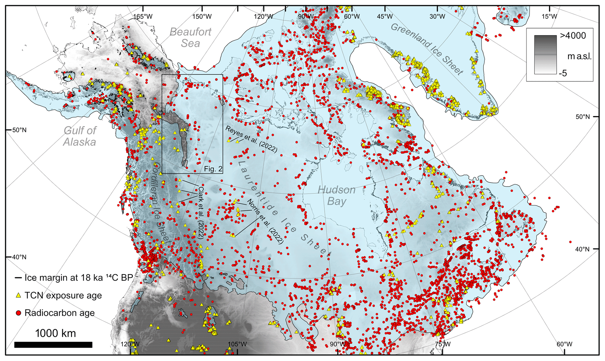
Figure 1The Last Glacial Maximum (18.0 ka 14C/21.1 ka cal BP) extent of the North American Ice Sheet Complex according to the reconstruction of Dalton et al. (2020). The yellow triangles (terrestrial cosmogenic nuclide exposure ages) and red dots (radiocarbon ages) show the distribution of dates constraining deglaciation. The expage compilation by Heyman (2022) was used to plot the distribution of terrestrial cosmogenic nuclide exposure ages, and the database of Dalton et al. (2020) was used to plot the distribution of radiocarbon ages.
Despite its relevance to meltwater routing and migration pathways during the last deglaciation, the dynamics and chronology of the NW LIS sector remain some of the most poorly constrained of the whole ice sheet (Fig. 1). Current ice sheet chronologies along the ∼500 km transect in the central Mackenzie Valley (Fig. 1) are loosely anchored by 20 minimum-limiting radiocarbon ages of varying quality and 16 early 36Cl cosmogenic dates (Duk-Rodkin et al., 1996). Recent advances in terrestrial cosmogenic nuclide (TCN) exposure dating have enhanced our ability to constrain the timing of deglaciation and have been widely applied to date the retreat of the LIS (Gosse and Phillips, 2001; Briner et al., 2006; Dunai, 2010; Balco, 2011). TCN exposure dating has been used to further constrain the timing of deglaciation for the sparsely dated central-western and southwestern sectors of the LIS (Fig. 1) (Clark et al., 2022; Norris et al., 2022; Reyes et al., 2022). However, the early deglaciation of the NW LIS is yet to be adequately constrained using this approach. Duk-Rodkin et al. (1996) used early TCN exposure dating methods to provide an age indication on the LIS maximum at ca. 30 ka, with a readvance phase at ca. 22 ka. These samples were never published in full, so it is not possible to recalculate these ages. The final deglaciation of the LIS from the central Mackenzie Valley occurred perhaps no later than ca. 13.0 ka cal BP according to minimum-limiting radiocarbon ages (Dyke et al., 2003; Dalton et al., 2020) (Figs. 1 and 2).
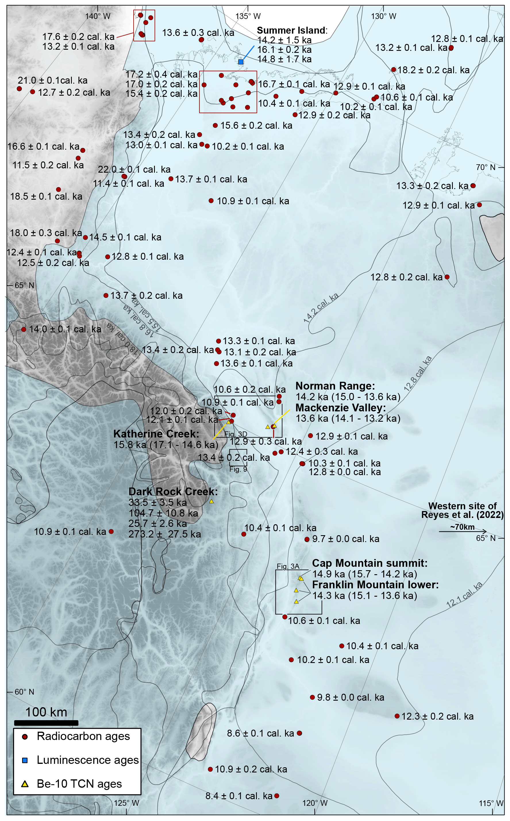
Figure 2The distribution of chronological constraints on the deglaciation of the NW sector of the Laurentide Ice Sheet. The pattern of deglaciation is depicted by grey lines, and the shaded blue area represents the local LGM limit at 18.0 ka cal BP (Dalton et al., 2020). For our new TCN exposure ages, we present the mean site deglaciation ages (2σ range) calculated from our Bayesian modelling. Radiocarbon ages were selected from the database of Dalton et al. (2020) and recalculated using the IntCal20 curve (Reimer et al., 2020). Radiocarbon ages in the red boxes have been grouped together; the ages next to the red boxes are the three oldest radiocarbon ages in the grouping. We only present the oldest OSL ages from post-glacial sediments in the Mackenzie Delta region (Bateman and Murton, 2006; Murton et al., 2007, 2010, 2015).
In this study, we reconstruct the deglaciation of the NW LIS in the central Mackenzie Valley region. We present 30 new 10Be TCN exposure dates from erratic boulders across six sites along the Mackenzie Valley between 63 and 65∘ N (Fig. 2). Our TCN exposure dates cover a range of latitudes and elevations which allow us to quantify ice sheet thinning along with lateral retreat rates. We integrate these data with the existing radiocarbon constraints in a Bayesian model that is consistent with regional chronological information on deglaciation. We also combine our revised ice sheet chronology with ice sheet model outputs from Gregoire et al. (2016) to quantify total ice volume loss and freshwater flux to the Arctic Ocean from a collapsing NW LIS during early deglaciation.
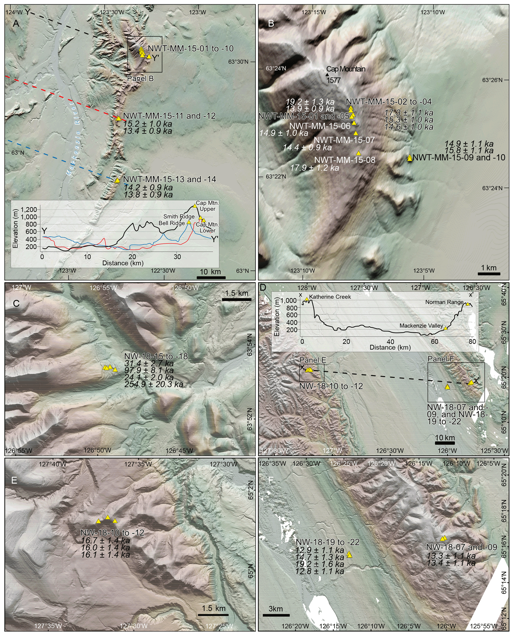
Figure 3(a) Location of the sampling sites in the Franklin Mountains. (b) Close-up of Cap Mountain, where samples NWT-MM-01 to 10 were collected along an elevation transect. (c) Close-up of the Dark Rock Creek site. (d) Location of the northern sampling sites. (e) Close-up of the Katherine Creek site, where samples NWT-18-10 to 12 were collected along the ridge. (f) Close-up of the Mackenzie Valley and Norman Range sites, where samples NWT-18-19 to 22 and samples NWT-18-07 to 09 were collected. Digital elevation model (DEM) courtesy of the Polar Geospatial Center (Porter et al., 2018).
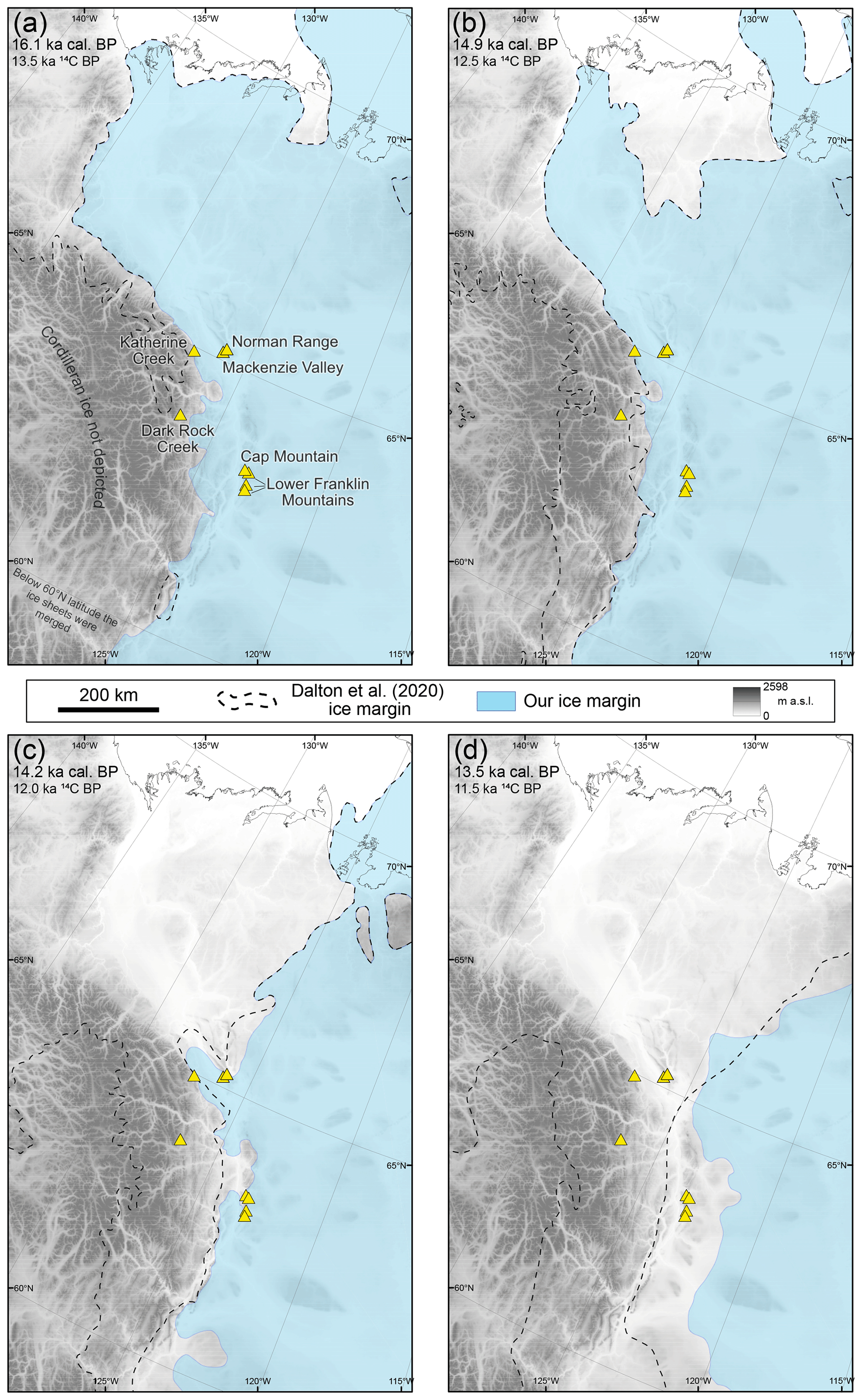
Figure 4Our ice margin retreat chronology compared to the reconstruction of Dalton et al. (2020). Yellow triangles indicate TCN exposure sampling sites. We do not depict the Cordilleran Ice Sheet in any of our reconstructions (a) Ice margin reconstruction at 16.1 ka cal BP. (b) Ice margin reconstruction at 14.9 ka cal BP. (c) Ice margin reconstruction at 14.2 ka cal BP. (d) Ice margin reconstruction at 13.5 ka cal BP.
Table 1Cosmogenic 10Be sample data and modelled surface exposure ages.

a Modern-day elevation as recorded in the field.
b The tops of all samples were exposed at the surface.
c Shielding factor is 1 for all samples.
d All uncertainties are reported at the 1σ level. Blank-corrected
ratios. See the Methods section for details on the level of blanks.
e Exposure ages were calculated with the online calculator formerly
known as CRONUS (Balco et al., 2008), version 3.0, constants 3.0.4
(http://hess.ess.washington.edu/, last access: February 2022). Full details of the
cosmogenic 10Be analyses and exposure age calculations are provided in
the Methods section.
f Exposure ages were calculated using the primary production rate
(Borchers et al., 2016) and none of the corrections outlined in the Methods section.
g Exposure ages calculated following our preferred approach, as
detailed in the Methods section. This includes the use of the primary
production rate (Borchers et al., 2016), a correction for glacial isostatic adjustment (GIA)-related
changes, and no correction for snow cover or atmospheric changes.
h Exposure ages calculated following the approach set out in Reyes et
al. (2022), using the Arctic production rate and the Lal–Stone scaling
method. A correction for GIA was made following the approach outlined in the
Methods section.
i Ages previously published in Reyes et al. (2022).
NA: not available.
2.1 TCN exposure dating
2.1.1 Site selection and sampling
We sampled 30 glacial erratic boulders of granite, sandstone, and quartzite lithologies from six different sites that span the LGM position of the NW LIS and the eastern section of the central Mackenzie Valley (Figs. 2, 3 and 4, Table 1). We chose two sites within the Mackenzie Mountains to date the start of deglaciation. At the Dark Rock Creek site (∼1375 m a.s.l.), we targeted a series of lateral meltwater channels incised by meltwater from the LIS as it extended up the Redstone River valley to Dark Rock Creek at the local LGM (Figs. 2 and 3c). At the Katherine Creek site, we collected samples from a ridgeline (∼1050 m a.s.l.) above Katherine Creek at the approximate LGM position (Fig. 3e) (Duk-Rodkin and Hughes, 1991). This site is slightly below the elevation limit of erratic boulder occurrence, which has been established as between 1160 and 1200 m a.s.l. (Duk-Rodkin and Hughes, 1991). The remaining four sites were in the eastern portions of the Mackenzie Valley at varying latitudes between ∼63 and ∼65∘ N and at a range of elevations so that we could use the 10Be dipstick approach to quantify the rate of ice sheet thinning (e.g. Koester et al., 2017; Small et al., 2019). We use the dipstick approach at two sites. First, at 65∘ N, ∼65 km east of the Katherine Creek site, we collected samples at the summit of the Discovery Ridge of the Norman Range (∼920 m a.s.l.) and on the adjacent Mackenzie Valley floor (∼200 m a.s.l.) (Fig. 3f). Second, at 63∘ N, we collected 10 samples transecting Cap Mountain, the highest peak of the Franklin Mountains (1577 m; samples ranging in elevation from 1479–814 m). Additionally, two pairs of samples were collected at the summit of the Smith and Bell ridges of the Franklin Mountains, ca. 20 and 40 km south of Cap Mountain, at about 1000 and 850 m a.s.l., respectively (Fig. 3a and b).
We took samples using a diamond blade cutoff saw and a hammer and chisel. At each site, we sampled a minimum of three erratic boulders. Boulder sampling followed a standard procedure which aimed to reduce the possibility of prior or incomplete surface exposure (Applegate and Alley, 2011; Balco, 2011, 2020). In particular, we preferentially sampled the surface of erratic boulders which were situated on stable ground away from steep slopes (Heyman et al., 2011), displayed a rounded shape suggesting a longer transport history by the ice sheet, exhibited limited evidence of surface weathering (Balco, 2011), and were large and well exposed above the ground surface (Heyman et al., 2016). Sampled boulders for TCN exposure dating should be exposed >1 m above the ground where possible. Limited boulder availability meant that some smaller boulders were sampled. These smaller boulders are more likely to be impacted by shielding from snow cover or to have been exhumed following the denudation of surface till cover, resulting in an exposure age which underestimates the true deglaciation age (Heyman et al., 2016). In our sampling area, the annual precipitation rates are very low (average snow depth of less than 30 cm; Government of Canada, 2019), meaning that snow cover is unlikely to be an issue. The majority of our samples were taken from high-elevation sites with very limited till cover, meaning the sampled boulders are unlikely to have been covered in till after deposition.
2.1.2 TCN sample preparation, analysis, and measurement
The samples were prepared as BeO targets at the CRISDal Lab, Dalhousie University. To concentrate sufficient (20 g) quantities of quartz from each sample, the following procedure was used: samples were cleaned, crushed, and ground, and the 250–355 µm fraction was rinsed, leached in aqua regia (2 h), and etched in a solution of 2:1 concentrated ACS-grade HF acid to deionised water, before mineral separation using combinations of froth flotation, Frantz magnetic separation, air abrasion, heavy liquids, and controlled digestions of non-quartz phases using hydrofluoric or hexafluorosilicic acids. When the quartz concentration was sufficiently pure (as determined optically and with < 100 ppm Al and Ti as determined on a 1 g aliquot with the lab's inductively coupled plasma optical emission spectroscopy, ICP-OES), approximately 35 wt. % of the dried quartz concentrate was removed in an ultrasonic bath with dilute HF as per Kohl and Nishiizumi (1992). The samples were spiked with approximately 240 µg of Be from BeCl2 carrier “Be Carrier B31 Sept 28, 2012” which was produced at CRISDal from phenacite sourced from the Ural Mountains, with an ICP-OES-measured average Be concentration of 282±5.64 µg mL−1 (replicated by Nathaniel Lifton at PRIME Lab with a measurement of 279 µg mL−1) and density of 1.013 g mL−1. The of the carrier was less than . Samples were then digested in a HF-HNO3 mixture, evaporated twice in perchloric acid, and treated with anion and cation column chemistry to isolate the Be2+. After acidifying with perchloric and nitric acid to remove residual B, Be(OH)2 was precipitated using ultrapure ammonia gas, transferred to a cleaned boron-free quartz vial, and carefully calcined in a Bunsen burner flame to a white oxide for over 3 min. The BeO was powdered, mixed 2:3 by volume with high-purity niobium powder (325 mesh), and packed into stainless-steel cathodes for measurement at the Center for Accelerator Mass Spectrometry, Lawrence Livermore National Laboratory (CAMS-LLNL). These measurements were made against the 07KNSTD3110 standard with a known ratio of = (Nishiizumi et al., 2007). Process blanks were also analysed and used to subtract 10Be introduced during target preparation and analysis. The process blanks had ranging from 2.7 to , so for all samples this correction was less than 1 % of the adjusted 10Be values.
2.1.3 Exposure age calculation
Exposure ages were calculated using the online calculator by Balco et al. (2008; version 3.0; constants 3.0.3) and are reported here using the time-dependent CRONUS LSDn production rate scaling of Lal (1991) and Stone (2000), using the “primary” calibration dataset of Borchers et al. (2016). Individual ages are reported to one significant figure with a 1σ external error (Balco et al., 2008), which considers systematic uncertainties in site production rate, and internal error, which includes the following random error sources, added in quadrature: (i) 1σ AMS precision in (atoms/atoms), which averaged 2.1 % and is the greater of the Poisson distributed statistic for the total number of counts on a target or the coefficient of variation about the mean after three, four, or five passes on each target; (ii) 1σ uncertainty in carrier concentration (µg mL−1), which includes uncertainty in density and is based on the greater of the 1 standard deviation of three measurements for a given wavelength or the standard deviation of the two wavelengths (313.042 and 234.861 nm) – carrier concentration uncertainty for “Be Carrier B31 Sept 28, 2012” was less than 2 % over nine measurements but is rounded to 2 %; and (iii) 1σ error in sample Be concentration (µg mL−1) as measured by ICP-OES, and error contributed by uncertainty in the process blank, which is calculated in the same manner as (ii). This approach differs from Reyes et al. (2022) and Clark et al. (2022), who used the Arctic production rate (Young et al., 2013) and the Lal–Stone scaling method (Balco et al., 2008). For comparison, we calculate our ages with both production rates and scaling factors in the Supplement (Tables S3, S4, S5, S6), describe the impact of different calculation approaches in the results section, and discuss the choice of production rate in Sect. 4.1.2.
Boulder surface erosion, snow and vegetation cover, atmospheric mass distribution variations during glacier–interglacial transitions, and elevation changes from GIA can all influence TCN production rates and therefore need to be considered when interpreting TCN exposure ages. The sampled coarse granitoid surfaces displayed grain-scale relief suggestive of surface erosion by grusification. We selected boulders without distinct weathering rinds, gnammas, rillen, or grus on the surrounding ground. Therefore, we assume surface weathering was limited to a few millimetres over the exposure period given the dry continental climate and lack of vegetation on the sampled surfaces. The region has low winter precipitation (161 cm average annual snowfall between 1981 and 2010, with average snow depth not exceeding 30 cm) (Government of Canada, 2019), and strong winds in the summit areas are expected to keep the top surfaces of erratics free of snow for most of the winter. Most of the sampling sites were situated above the tree line, with two sites covered by low-density boreal forest which would account for less than a 1 % decrease in production rate (Plug et al., 2007). As most of the exposure ages postdate the LGM, the influence of katabatic winds and other atmospheric dynamics changes associated with the LIS and CIS ice sheets would have been brief and therefore limited (Staiger et al., 2007). Previous studies that have investigated the impact of changes in atmospheric mass distribution have found that it results in a younger exposure age calculation, but the impact is minimal (∼4 % of the GIA correction, Cuzzone et al., 2016; 1 %–5 % of the GIA correction, Ullman et al., 2016; ∼1 % of the GIA correction, Dulfer et al., 2021). Coupled with the absence of any model at a suitable resolution, we choose not to make corrections for changes in the atmosphere. We therefore do not adjust TCN production rates for erosion, snow or vegetation cover, or atmospheric changes during exposure as any effects are likely to be minimal and have large uncertainties. As more research on local temporal variations in atmospheric dynamics in deglaciating regions provides more insight, recalculations of these (and other) TCN exposure ages may be necessary (Jones et al., 2019).
In contrast, the effect of GIA following the deglaciation of the continental ice sheets is relatively well constrained in the Mackenzie Valley, compared to the changes in the atmospheric composition (Peltier et al., 2015; Lambeck et al., 2017; Gowan et al., 2021). A correction is needed to account for how atmospheric shielding varies as boulders are raised from lower elevations to their present-day elevations (Jones et al., 2019). The magnitude of GIA varies among our sampling sites, so a correction for GIA-induced change is important to ensure an internally consistent dataset (Fig. S1). In addition, recent studies in adjacent regions of the LIS also included a GIA correction (Norris et al., 2022; Reyes et al., 2022), and, hence, to ensure comparability with these datasets, we apply a correction for GIA-related changes to our dataset as well. The previously mentioned changes in atmospheric conditions following deglaciation work against the impact of GIA on calculated exposure ages, but the impact on exposure ages is likely an order of magnitude lower than that of GIA-induced impacts (Staiger et al., 2007; Cuzzone et al., 2016; Ullman et al., 2016; Dulfer et al., 2021).
We performed a sensitivity test to determine the impact of different GIA models on the exposure ages in Octave v6.4.0 using the expage-201912 calculator, an open-source script based on the equations of the CRONUS calculator (Table S1 and Fig. S1). Based on each model, this tool identifies the timing of ice-free conditions and then calculates the influence of GIA-induced elevation change on the TCN exposure age every 500 years since the site became ice-free. The ICE-6G model of Peltier et al. (2015) has the largest GIA response of the three models (up to 550 m elevation change over the past 15 kyr), with the ANU model of Lambeck et al. (2017) having an intermediate GIA response (up to 300 m elevation change over the past 15 kyr) and the model of Gowan et al. (2021) having the smallest GIA response (up to 100 m elevation change over the past 15 kyr) (Fig. S1). Following this, we selected the Lambeck et al. (2017) model as the most suitable for calculating GIA corrections for two main reasons: (1) the model resolution of Lambeck et al. (2017) is higher (0.25×0.25∘) compared to the other two models (1×1∘) and (2) the region-specific nature of the Lambeck et al. (2017) model means that it is tuned to empirical data from our study region. We believe these two points make this model most appropriate for our use. Additionally, the ice sheet reconstruction of Lambeck et al. (2017) includes the two assumptions that the Ice-Free Corridor did not open before 13 ka and that there was rapid deglaciation of the LIS during the Bølling–Allerød period, which are broadly aligned with our new chronological constraints. We then calculated the GIA correction following the method of Norris et al. (2022). First, we identified when a site became ice-free according to the model of Lambeck et al. (2017). Then, we extracted the change in elevation relative to sea level (ΔRSL) data of Lambeck et al. (2017) for each site at 500-year time steps. This effectively tells us the amount of GIA-related elevation change at each site for each 500-year time step. This allowed us to calculate an average change in elevation (ΔRSL) for the time since deglaciation. We then corrected the modern elevation of each sample by the average change in elevation (ΔRSL) for the site, resulting in an average site elevation since deglaciation. This GIA correction makes the ages between 0.1 % and 3.5 % older depending on the site and GIA history (Table 1).
2.1.4 Bayesian age modelling
To reduce the uncertainties of exposure ages and support outlier identification, we combined our new TCN exposure dates within Bayesian chronologies using OxCal v4.4 (Bronk Ramsey, 2017). These chronologies followed an age–elevation prior model (Buck et al., 1996), which assumes higher elevations were deglaciated before lower elevations, and therefore accurate exposure dates from these sites must be older than exposure dates from lower elevations (e.g. Jones et al., 2015; Small et al., 2019).
Following this prior model, we developed two uniform phase models that included groups of TCN exposure ages and minimum-limiting radiocarbon dates within sequential phases (Bronk Ramsey, 2009a). TCN exposure ages were input to the model using the external error while radiocarbon dates were input using the analytical uncertainty reported by the original authors. The Bayesian models were run interactively using different approaches for outlier detection. OxCal enables the statistical detection of potentially outlying dates in two main ways, either using the “agreement index” (a measurement of convergence between the unmodelled and modelled probability distributions of individual ages or the model as a whole) or the “outlier model” command (an outlier analysis that progressively down-weighs spurious dates) (Bronk Ramsey, 2009b). In each case, the first model iteration was run without the outlier function in order to assess overall and individual agreement indices. If the overall agreement index of the model was below the 60 % threshold suggested by Bronk Ramsey (2009b), TCN exposure dates with an individual agreement index of <60 % were considered for rejection in subsequent model runs. The next model iteration was run using a general outlier model which uses a Student t distribution on a timescale of 1–10 000 years (Bronk Ramsey, 2009b). In this model, each TCN exposure date was assigned 0.1 prior probability of being an outlier (i.e. 1 in 10) while flagging potentially outlying dates. Our Bayesian model for the northern sites also included radiocarbon dates. These radiocarbon dates are from post-glacial delta and lake sediments which must postdate our exposure age sampling sites and therefore provide a minimum timing of deglaciation. These radiocarbon ages do not follow our age–elevation prior model but can be placed in order as they are from sites which must have deglaciated after our northern sites. Radiocarbon dates were assigned a 0.05 prior probability of being an outlier (i.e. 1 in 20) and inserted into the models using the before function which considers dates as minimum (terminus ante quem) age controls only (Bronk Ramsey, 2009b). The final model iteration was run using the same outlier model parameters as the second model iteration, but with the exclusion of TCN exposure dates that fell substantially below the 60 % agreement index threshold in the first model iteration. The Bayesian syntax is provided in the Supplement (Figs. S7 and S8).
2.2 Compilation of existing chronological constraints
Radiocarbon dating of organic material can be used to constrain the timing of deglaciation, although it is subject to uncertainties inherent to the method. The time lag between deglaciation and the accumulation of organic material means that radiocarbon ages can only serve as a minimum constraint on the timing of deglaciation. We selected all ages relating to the deglaciation of the NW LIS from the database of Dalton et al. (2020) (Table S2). We recalibrate the radiocarbon dates using the online calibration tool Calib v8.2 with the updated IntCal20 Northern Hemisphere calibration curve (Reimer et al., 2020; Stuiver et al., 2021). We provide an updated version of the Dalton et al. (2020) database (Table S2) and refer to the median calibrated ages for the rest of this discussion.
Similar to radiocarbon dating, luminescence dating from post-glacial sites can provide a minimum age on when an area became ice-free. We compile previously published deglacial luminescence ages (optically stimulated luminescence, OSL; and infrared stimulated luminescence, IRSL), which within the study region are only located at the Summer Island site in the north (Bateman and Murton, 2006; Murton et al., 2007, 2010, 2015) (Fig. 2). We manually select the oldest dates when building our chronology, as they are most relevant to reconstructing the timing of deglaciation. Post-glacial features (e.g. dunes) have also been previously dated with OSL outside of our study area on the bed of the former W LIS (Wolfe et al., 2004, 2006, 2007; Munyikwa et al., 2011); we refer to these in the discussion but do not include them in Table S2.
Surface exposure dating allows for direct dating of fresh rock surfaces emerging during deglaciation, without the time lags inherent to radiocarbon dating. No TCN exposure dates have been fully published that would date the deglaciation within our study area. Early work in TCN exposure dating by Duk-Rodkin et al. (1996) presents a single figure with 36Cl exposure ages, ranging from 32 to 14 ka, which constrain the LIS limits in the Mackenzie Mountains to the late Wisconsinan (Marine Isotope Stage 2). However, the calculated ages and the full details of sample analysis were not published for these samples, which are therefore not possible to recalculate. In addition, our understanding of the calculation of TCN exposure ages has advanced considerably since these ages were published. As a result, these ages are not comparable to our data in their original form, and so we do not refer to them any further.
2.3 Modelling ice sheet saddle collapse
We use the ice sheet model simulations of Gregoire et al. (2016) to derive information on plausible ice sheet evolution in the CIS–LIS saddle region during deglaciation. Gregoire et al. (2016) ran an ensemble of simulations of the North American Ice Sheet Complex (NAISC) using the Glimmer-CISM thermodynamic ice sheet model. The model runs span the range of uncertainties in model input parameters, including the ice sheet flow factor, the geothermal heat flux, the basal sliding parameter, the mantle relaxation time, positive degree day factors, and the atmospheric lapse rate.
The ice sheet mass balance was calculated using a positive degree day mass balance scheme, forced with output from two general circulation models (GCMs). Here, we present further analysis of simulations from the Cano ensemble of ice sheet simulations (see Gregoire et al., 2016). These simulations use the TraCE 21 ka climate simulations to produce an anomaly forcing, correcting for the present-day model biases in the climatology of the GCM CCSM3. The deglacial forcing for Cano is calculated in this way:
where T is surface temperature (∘C), P is precipitation (mm d−1), H is orographic elevation in the model (metres) at the present day (PD) or corresponding to the reanalysis (clim), γ is the lapse rate (−5 ∘C km−1), x and y represent the latitude/longitude spatial dimensions (metres), m is an index for the months of the year (1–12; January–December), and t is the time (years). This climate forcing simulates warming at 14.7 ka, during the Bølling–Allerød interval, allowing the ice sheet simulations to span a reasonable deglaciation pattern.
The ensemble produces a large range of results. To only analyse the most realistic simulation, Gregoire et al. (2016) applied constraints on the ice extent and volume, referring to the resultant subset of 25 simulations as “not ruled out yet”. We focus on these “not ruled out yet” simulations selected by Gregoire et al. (2016) for matching constraints on ice sheet volume and area. We apply a further requirement that the Franklin Mountains region should not have deglaciated prior to 16 ka, in agreement with the new TCN exposure age data presented here, leading to a selection of 15 simulations. For each run in the selected Cano ensemble, we identify the timing of the peak ice volume loss and calculate the equivalent sea level contribution from the saddle region over a 340-year period centred around the maximum rate of volume loss (Fig. 5b), assuming an ocean area of 360 768 600 km2.

Figure 5(a) Simulated LIS surface elevations at the Franklin Mountains, 18–12 ka, in the 15 selected simulations. Shaded areas indicate the past time periods discussed in this study. (b) Sea level flux from the CIS–LIS saddle area. Black points show the point of maximum sea level flux for each simulation. The grey curve shows the sea level flux evolution for one simulation (Cano_34,; peak marked by a cross), with the 340-year period of peak sea level flux in red. (c) Ice thickness at 15 ka for one simulation (Cano_34), with grey contours every 500 m from 1000 m of ice thickness. The X–X′ line marks the transect used in panel (e), the red dot marks our southern sampling sites in the Franklin Mountains where the 10Be samples were collected, and the dashed rectangle marks the CIS–LIS saddle area used for calculations (same in panel d). (d) Surface mass balance (SMB) of the North American Ice Sheet Complex at 16 ka (Cano_34). Dark and light purple contours mark equilibrium line at 16 and 14 ka, respectively, showing the change in SMB that resulted in the CIS–LIS saddle collapse. (e) A transect through the CIS–LIS saddle (Cano_34), at 1000-year intervals from 18 ka (greatest extent) to 12 ka (smallest extent). The black curve shows topography and the grey curves successive ice surfaces, with dashed lines indicating 500-year intervals during the period of most rapid ice sheet thinning.
In this section, we briefly describe our sites and report the calculated exposure ages. Detailed information on each sample is provided in Table 1, including exposure age calculations with and without the GIA correction. From here, we refer only to calculated exposure ages corrected for GIA, unless specified otherwise. First, we describe the results of our TCN exposure age calculations, and then we provide a description of the results from our Bayesian models.
3.1 Dark Rock Creek
At Dark Rock Creek (Fig. 3c) we sampled four large angular quartzite erratics which appeared to originate from local bedrock (NW-18-15 to NW-18-18; Fig. S2v–y). These erratics were all located on the raised ground between a series of lateral meltwater channels that were cut at the margin of the LIS (Fig. 3c). The resulting TCN 10Be exposure ages from Dark Rock Creek are poorly clustered and cannot be used to infer an age for the LIS meltwater channels at this site (Table 1). The age spread and tendency towards older ages at this site suggest a strong TCN signal resulting from prior exposure. As the sampled boulders all appeared to be of local material, they likely experienced short transport distances and minimal erosion leading to inheritance. Due to the un-replicated results of this site, we do not refer to data from Dark Rock Creek further when building our chronology of the LIS deglaciation.
3.2 Katherine Creek
At Katherine Creek, we sampled five granite erratics along a ridgeline above the western Mackenzie Valley (NW-18-10 to NW-18-14; Fig. 3e; Fig. S2s–u). Two of these samples could not be analysed due to insufficient quartz content (NW-18-13 and NW-18-14). The samples were all collected from within 3 km of each other and at a similar elevation (1048–1075 m a.s.l., modern-day elevation). They resulted in exposure ages of 16.7±1.4 ka (NW-18-10), 16.0±1.4 ka (NW-18-11), and 16.1±1.4 ka (NW-18-12). This site is located near the ice sheet margin so there is little GIA-related elevation change (Fig. S1) and minimal impacts on our calculated exposure ages (Table 1; Fig. 6b).
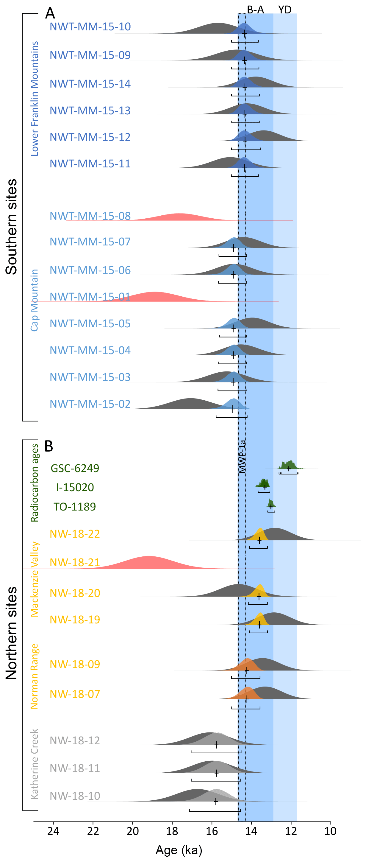
Figure 6(a) Phase model from the Bayesian modelling showing the exposure age probability for the southern sites. The dark grey probability distribution plots relate to the age distribution of individual TCN exposure ages. The coloured plots indicate the modelled age probability distribution from our Bayesian modelling. Black crosses indicate the median modelled age, with uncertainty. The red plots indicate ages which were identified as outliers within the model. Full information on the Bayesian modelling is provided in Figs. S3 and S4 and Tables S4 and S5. Shaded blue areas indicate the timing of the Bølling–Allerød interval (B–A) and the Younger Dryas interval (YD). (b) Phase model from the Bayesian modelling showing the exposure age probability for the northern sites. The red plots indicate ages which were identified as outliers within the model. The probability distribution of the three oldest radiocarbon ages which constrain our model is displayed in dark green.
3.3 Norman Range and the Mackenzie Valley
The Norman Range forms the northernmost extension of the Franklin Mountains, with approximately 700 m of relative relief over the adjacent eastern Mackenzie Valley (Fig. 3d and f). We sampled three granite erratics from the summit of Discovery Ridge (NW-18-07 to NW-18-09; Fig. S2q–r; Table 1; Fig. 6b). One sample had insufficient quartz to be analysed (NW-18-08). The remaining two boulders returned exposure ages of 13.3±1.1 ka (943 m a.s.l.) and 13.4±1.1 ka (924 m a.s.l.). We sampled four erratic boulders from the floor of the Mackenzie Valley ∼15 km west of the summit samples (NW-18-19 to NW-18-22; 192–207 m a.s.l.; Fig. S2z–ac); three of the boulders were composed of granite (NW-18-20 to NW-18-22) and one was pink sandstone (NW-18-19). These samples returned exposure ages of 12.9±1.1 ka (NW-18-19), 14.7±1.3 ka (NW-18-20), 19.2±1.6 ka (NW-18-21), and 12.8±1.1 ka (NW-18-22). The influence of GIA at this site is limited to a maximum of 0.2 kyr for our non-outlier samples, due to the close proximity of the LGM ice sheet margin (Fig. S1; Table 1).
3.4 Cap Mountain and the lower Franklin Mountains
In the Franklin Mountains, we sampled 14 boulders across two separate elevation groups which occupy distinct elevations (Fig. 3a and b). At our upper-elevation site, located near the summit of Cap Mountain, we sampled eight granite erratics between 1279–1479 m a.s.l. (NWT-MM-15-01 to NWT-MM-15-08) (Table 1; Fig. 6a). The sampled boulders were all highly rounded and rested directly on the local bedrock or, where the bedrock was transitioning into a poorly developed blockfield, lay between the local blocks and boulders. The exposure ages at this site range from 19.2±1.3 ka (NWT-MM-15-01) to 14.4±0.9 ka (NWT-MM-15-07). A further six boulders were sampled across the lower Franklin Mountains group. This includes two boulders from ∼2 km east of the summit of Cap Mountain, at an elevation of 832 m a.s.l. (NWT-MM-15-09) and 814 m a.s.l. (NWT-MM-15-10). These returned exposure ages of 14.8±1.1 ka and 15.8±1.1 ka, respectively. Two more boulders were sampled from the summit of the Smith Ridge, which is a ridgeline in the Franklin Mountains, approximately 20 km south of Cap Mountain. These boulders were located at 987 m a.s.l. (NWT-MM-15-11) and 985 m a.s.l. (NWT-MM-15-12), with exposure ages of 15.2±1.0 ka and 13.4±0.9 ka. The final two boulders were sampled on the summit of the Bell Ridge, which is located approximately 20 km south of the Smith Ridge. These boulders were located at 854 m a.s.l. (NWT-MM-15-13) and 847 m a.s.l. (NWT-MM-15-14). The exposure ages were calculated as 14.2±0.9 ka and 13.8±0.9 ka. We acknowledge that there is some distance between the samples of the lower-elevation group; however, given the regional ice sheet deglaciation history and similar topographic setting of the sampling locations (Mas e Braga et al., 2021), the ∼40 km horizontal distance between the furthest sites is relatively minor and beyond the precision of TCN exposure dating.
3.5 Bayesian models
The first uniform phase model included exposure ages from study sites at Katherine Creek, Norman Range, and the Mackenzie Valley, grouped within three sequential phases (Fig. S3). One TCN exposure date was removed from the model (NW-18-21). This date is several thousand years older than any of the other exposure ages used in the model and could be confidently excluded using either the OxCal outlier analyses or manual rejection following age–elevation relations. Since the modelled ages all display a normal distribution, we calculate a mean average for each site to provide a best estimate of the timing of deglaciation. Based on our vetted model (Fig. 6b and model 3 in Fig. S3 and Table S3), our results suggest that Katherine Creek was deglaciated at ca. 15.8 ka (with a 2σ maximum–minimum range 17.1–14.6 ka). Following this, the summit of the Norman Range (∼900 m) became ice-free at ca. 14.2 ka (15.0–13.6 ka). Finally, the Mackenzie Valley floor was deglaciated at ca. 13.6 ka (14.1–13.2 ka). Alternatively, a more conservative approach could use the median value of end boundaries between phases for each site to provide a minimum estimate on the timing of ice-free conditions. We provide the information from our Bayesian model outputs in Table S3 and Fig. S7. In comparison, the exposure age calculation using the Arctic production rate and the Lal–Stone scaling suggests a mean site deglaciation age of ca. 17.1 ka (18.2–16.1 ka) for Katherine Creek, while the Norman Range deglaciated at ca. 14.9 ka (15.6–14.2 ka) and the Mackenzie Valley at ca. 14.2 ka (14.8–13.6 ka) (Table S5; Fig. S5).
The second model included exposure ages from study sites at Cap Mountain summit and lower Franklin Mountains, grouped within two sequential phases (Fig. S4). Within model iteration 1, two TCN exposure dates (NWT-MM-15-01 and NWT-MM-15-08) had individual agreement index values substantially <60 % and reduced the overall agreement index of the model to <60 %. These were rejected from model iteration 3. Results from this model indicate a mean average timing of deglaciation of ca. 14.9 ka (15.7–14.2 ka) for our upper-elevation samples near the summit of Cap Mountain (∼1450 m). The lower-elevation sites (∼800 m) became ice-free around 600 years later, at ∼14.3 ka (15.1–13.6 ka). Full information from our Bayesian model outputs is available in Table S4 and Fig. S8. Exposure age calculation using the Arctic production rate results in a mean site deglaciation age of ∼17.0 ka (18.5–15.3 ka) for the Cap Mountain summit site, which is considerably older than our calculation. The calculation of exposure ages using the Arctic production rates results in lower uncertainties and a greater age spread, which means the Bayesian model cannot easily reconcile all of the available age constraints (Figs. 8, S6; Table S6). The lower Franklin Mountains site deglaciated at ∼14.9 ka (15.6–14.2 ka) using this calculation method.
4.1 Implications for the regional retreat pattern
4.1.1 Amendments to the existing ice margin retreat chronology
The existing ice margin chronology of Dalton et al. (2020) in the Mackenzie Valley largely follows the models of Lemmen et al. (1994) and Dyke et al. (2003) and portrays the eastern ridges of the Mackenzie Mountains at 63∘ N as glaciated until ∼15.5 ka cal BP (thousand calibrated years before 1950 CE; Fig. 2). Following initial retreat, ice persists in the central Mackenzie Valley until ∼13.5 ka cal BP, with the NW LIS margin abutting against the slopes of the Mackenzie Mountains (Fig. 4). The Dalton et al. (2020) ice margin chronology is based on minimum-limiting radiocarbon ages, which for this region vary between 11.5 and 9.0 ka 14C (13.4 and 10.3 ka cal BP). In contrast, our ages indicate an earlier start of deglaciation and a change in the retreat pattern and style. We present a new chronological model for the deglaciation of the NW LIS in Fig. 4; a full justification of our changes to the ice margin pattern is described in the Supplement, Document 1. To allow for a more direct comparison of ice retreat, we use time slices from the previous reconstructions of Dyke et al. (2003) and Dalton et al. (2020).
The new 10Be ages indicate deglaciation of the eastern summits of the central Mackenzie Mountains began at ∼ 15.8 ka (17.1–14.6 ka) (Fig. 4a). This is compatible with existing data on the timing of advance and retreat of the NW LIS further north in the Richardson Mountains, where radiocarbon ages indicate that the LIS reached its maximum sometime after ∼19.1 ka cal BP (18.9–19.4 ka cal BP) and began to retreat from its maximum position by ∼16.6 ka cal BP (Kennedy et al., 2010; Lacelle et al., 2013). Further north, the LIS reached its short-lived maximum in the Mackenzie Delta region between 16.6 and 15.9 ka (Bateman and Murton, 2006; Murton et al., 2007, 2015). These constraints are closely aligned and suggest that the initial deglaciation of the NW LIS at ∼16 ka was broadly synchronous from the Mackenzie Delta and Richardson Mountains to the Mackenzie Mountains.
Following the start of deglaciation, the NW LIS margin at 63–65∘ N remained stable as the ice sheet occupied the Mackenzie Valley with the ice margin pressed against the eastern slopes of the Mackenzie Mountains during a period of ice sheet thinning. The highest summits (∼ 1500 m) of the southern Franklin Mountains became ice-free at ∼ 14.9 ka (15.7–14.2 ka) and their lower elevations (∼900 m) by ∼14.3 ka (15.1–13.6 ka) (Fig. 4b and c). Compared with the reconstruction of Dalton et al. (2020) and Dyke et al. (2003), these constraints suggest an earlier deglaciation of the Franklin Mountains at 63∘ N by around 1000 years. Exposure ages from ∼1000 m elevation in the Rocky Mountains at 58.7∘ N indicate LIS deglaciation at 14.4±0.6 ka (Clark et al., 2022). OSL ages from dune fields provide a minimum constraint on deglaciation and suggest the separation of the LIS and CIS as early as 15 ka in central Alberta (Munyikwa et al., 2011), with ice sheet retreat to the south of Great Slave Lake likely by ∼13.4 ka (Wolfe et al., 2007; High Level, Alberta; Norris et al., 2021) and definitely by 10.5 ka (Wolfe et al., 2004; Sandy Lake, Alberta). These data are all consistent with our new chronological constraints. Similar shifts to an earlier timing of deglaciation from existing radiocarbon-based chronologies have been suggested by recent TCN exposure dating studies (Norris et al., 2022; Reyes et al., 2022).
At 65∘ N, ice remained over the Norman Range (∼ 900 m a.s.l.) until ∼14.2 ka (15.0–13.6 ka) and at lower elevations (∼200 m a.s.l.) in the Mackenzie Valley until ∼ 13.6 ka (14.1–13.2 ka) (Fig. 4d). This aligns with previous studies which suggested that the Mackenzie Valley must have been ice-free by the Younger Dryas time period (12.9–11.6 ka) (Smith, 1994; Gowan, 2013; Gowan et al., 2016; Dalton et al., 2020). Nearby radiocarbon dates from the Little Bear River delta (∼50 km south) suggest that Glacial Lake Mackenzie occupied this area at 13.4±0.17 ka cal BP (13.1–13.8 ka cal BP; I-15020; Smith, 1992). Ice margin retreat continued to the east of our study area, reaching the Canadian Shield at ∼115.7∘ W, by at least 12.6 ka (11.8–13.4 ka) (Reyes et al., 2022).
Our new age constraints necessitate a revision of the ice margin retreat pattern and timing. Our TCN exposure ages suggest that the Franklin Mountains at 63∘ N were deglaciated down to ∼900 m by ∼14.3 ka, around 1000 years earlier than in the reconstruction of Dalton et al. (2020). The Norman Range at 65∘ N and a similar elevation (∼900 m) deglaciated at broadly the same time, ∼14.2 ka, with the Mackenzie Valley at ∼200 m glaciated until 13.6 ka. The age constraints at 65∘ N are broadly consistent with the existing radiocarbon reconstruction of Dalton et al. (2020). These changes to the chronology result in a shift in the retreat pattern compared with past reconstructions, which suggested ice retreated to the south, up the Mackenzie Valley. We find no evidence that the deglaciation of the Mackenzie Valley region around 63∘ N lagged the timing of deglaciation around 65∘ N, as suggested by previous reconstructions (Dalton et al., 2020). Instead, we propose that the retreat of the LIS across this region was broadly synchronous and to the east, with the final deglaciation involving topographically constrained ice lobes occupying lower elevations (Fig. 4).
4.1.2 A comparison of different approaches to exposure age calculation
The use of different calculation methods or calibration data when calculating TCN exposure ages can result in changes in the exposure age. A range of approaches have been used when calculating exposure ages in recently published datasets for the W LIS, including the use of different production rates, scaling methods, and GIA corrections (cf. Clark et al., 2022; Norris et al., 2022; Reyes et al., 2022). Issues arise when trying to compare exposure age datasets with different calculation approaches as the published deglaciation ages are often incompatible. Reyes et al. (2022) suggest the NW LIS retreated to the Canadian Shield, to the east of our study area, by 13.9±0.6 ka (Fig. 1), conflicting with our new exposure ages in the Mackenzie Valley region. Reyes et al. (2022) used the Arctic production rate (Young et al., 2013), the Lal–Stone scaling method (Balco et al., 2008), and a modelled GIA correction in their exposure age calculations. In Table 1, we provide exposure ages calculated following our preferred method and following the method detailed in Reyes et al. (2022). The GIA correction of Reyes et al. (2022) is based on simulations from Tarasov et al. (2012). Instead, we apply the GIA correction described in our Methods section and following the method of Norris et al. (2022). Our GIA correction results in exposure ages which are ∼3.5 %–4 % younger for the sites presented in Reyes et al. (2022).
The choice of production rate has the strongest influence on the calculated exposure age, with the scaling factor having a lesser effect. Exposure ages calculated using the Arctic production rate (Young et al., 2013) instead of the primary calibration dataset of Borchers et al. (2016) are ∼8.5 % older. The choice of scaling method only has ∼2 % influence on the calculated exposure age. The Arctic production rate calibration dataset is composed of 18 samples from five sites in west Greenland and east Baffin Island (Young et al., 2013). These samples occupy a narrow latitudinal range (69.1–69.8∘N), low elevations (65–350 m), and are relatively young (8.2–9.2 ka). While our sites are situated in the subarctic (63–65∘ N), the other characteristics of our sites make it inappropriate to use the Arctic production rate calibration dataset to calculate our exposure ages. Most importantly, multiple sites are situated around or above 1000 m elevation and may be as old as 16–17 ka. The primary calibration dataset of Borchers et al. (2016) includes 47 samples at five sites that cover a range of elevations (∼130–4900 m), ages (9.6–18.3 ka), and latitudes (43∘ S–57∘ N), which we think are more representative of the range of sites in this study.
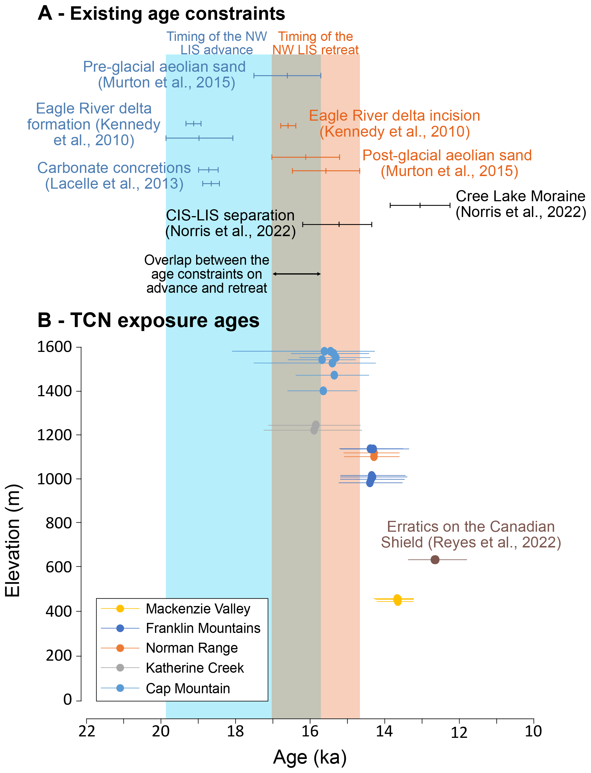
Figure 7Comparison of our reconstruction of the timing of deglaciation based on the Bayesian model outputs with existing age constraints. The shaded orange area indicates timing of retreat of the NW LIS including dating method uncertainties, and the shaded blue area indicates the timing of advance of the NW LIS including dating method uncertainties based on the age constraints in panel (a). (a) Existing age constraints on the timing of NW LIS advance and retreat to the LGM. The chronological constraints of the advance of the NW LIS to the LGM are shown as blue lines, and the constraints on the timing of retreat from the LGM are shown in orange. The timing of deglacial events from the multi-chronometer Bayesian model reconstruction of the SW LIS is shown as black points (Norris et al., 2022). Points in this panel are not placed in an elevation sequence. (b) Age–elevation plot using the modelled age distribution output of Bayesian model 2 and 5 (Figs. S3 and S4; Tables S3 and S4). The exposure ages were calculated using the primary calibration dataset (Borchers et al., 2016), LSDn scaling, and a correction for glacioisostatic adjustment (GIA; as described in Sect. 2.1.3).
The primary calibration dataset (Borchers et al., 2016) produces results which are compatible with the existing chronological constraints on the deglaciation of the NW LIS (Fig. 7). The NW LIS was advancing to the Richardson Mountains around 18.6 ka (Kennedy et al., 2010; Lacelle et al., 2013) and to the Mackenzie Delta possibly as late as ka (Murton et al., 2015). The local LGM was short-lived, with retreat beginning by ∼16 ka in the Richardson Mountains and Mackenzie Delta (Bateman and Murton, 2006; Kennedy et al., 2010; Murton et al., 2015). The eastern peaks of the Mackenzie Mountains, around Katherine Creek, should deglaciate shortly after this, while Cap Mountain, in the Franklin Mountains, should deglaciate even later. However, exposure ages calculated with the Arctic production rate are in conflict with this reasoning, as they suggest deglaciation at Katherine Creek began as early as 17.1 ka (18.2–16.1 ka), with Cap Mountain ice-free at approximately the same time (17.0 ka; 18.5–15.3 ka). Therefore, we favour the primary calibration dataset of Borchers et al. (2016) for calculating the exposure ages in this study as it results in a deglacial model which is consistent with other existing geomorphological and chronological constraints.
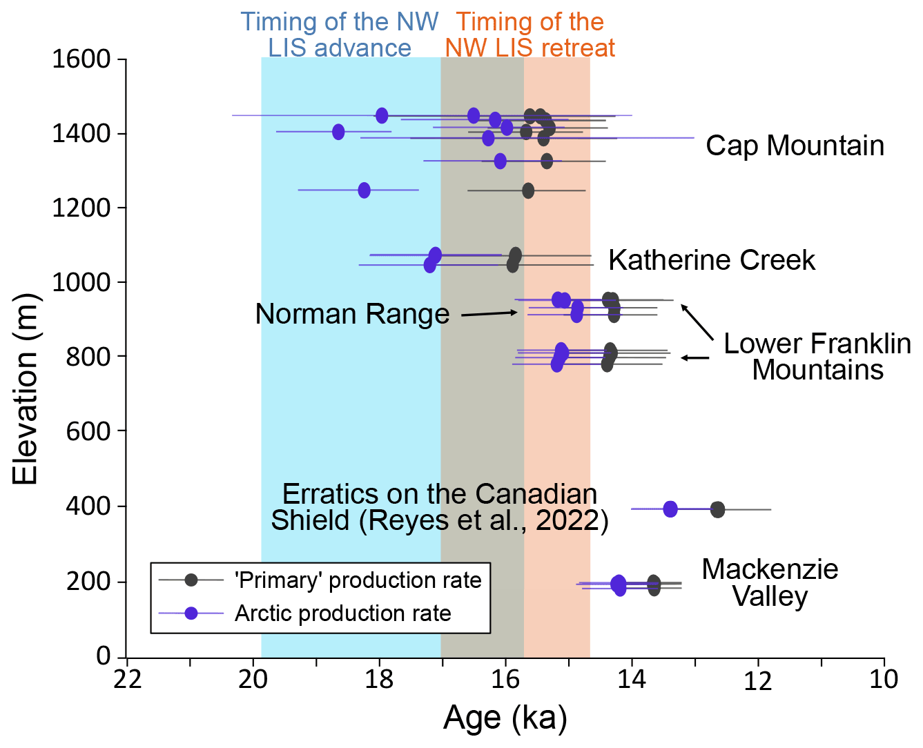
Figure 8The influence of the exposure age calculation approach on the reconstructed age of deglaciation. Shaded orange and blue areas are based on the age constraints in Fig. 7. The primary production rate exposure ages were calculated using the primary calibration dataset (Borchers et al., 2016), LSDn scaling, and a correction for glacioisostatic adjustment (as described in Sect. 2.1.3) and plotted using the modelled age distribution output of Bayesian model 2 and 5 (Figs. S3 and S4; Tables S3 and S4). The Arctic production rate exposure ages were calculated using the Arctic production rate (Young et al., 2013), Lal–Stone scaling, and a correction for GIA (as described in Sect. 2.1.3) and plotted using the modelled age distribution output of Bayesian model 8 and 11 (Figs. S5 and S6; Tables S5 and S6). The wide spread of modelled ages for the Cap Mountain site is a result of the smaller uncertainties associated with exposure ages calculated with the Arctic production rate.
Regardless of the chosen calibration dataset, we are able to make two important contributions to the regional deglaciation chronology. First, irrespective of production rate, there is a robust trend indicating much earlier deglaciation than has been previously considered for the central Mackenzie Valley (Dyke et al., 2003; Dalton et al., 2020). Using the Arctic production rate (Young et al., 2013) produces a deglacial chronology that is largely too old when compared to the existing age constraints (Fig. 8). Using the primary production rate (Borchers et al., 2016) produces mean site ages which are ∼8 % younger than mean site ages calculated using the Arctic production rate. The deglacial chronology calculated using the primary production rate is more compatible with the existing geochronological constraints (Figs. 7 and 8). Second, both production rates produce a rapidly thinning LIS in the study area, with thinning rates beyond the resolution of TCN exposure dating (Figs. 7 and 8). In both models, ice sheet thinning starts before and continues through the Bølling–Allerød interval, in agreement with the model simulations of Gregoire et al. (2016) (Fig. 6). The majority of ice sheet thinning occurs within the Bølling–Allerød interval when using the primary production rate, whereas a substantial amount of melt occurs before the Bølling–Allerød when using the Arctic production rate.
4.2 Implications of ice-free Mackenzie Valley for species migration and meltwater routing
4.2.1 Opening of the Ice-Free Corridor and faunal migration
The exact timing of the opening of the IFC is contentious. Depending on the chosen chronological constraints and degree of scrutiny of the available data, it has been suggested the IFC may have been viable as early as 14.9 ka or as late 12.6 ka (Jackson et al., 1997; Heintzman et al., 2016; Pedersen et al., 2016; Potter et al., 2018; Froese et al., 2019; Margold et al., 2019). A primary migration route along the west coast of North America, termed the Pacific coastal route, has been suggested as an alternative to the IFC for early humans (Fladmark, 1979; Braje et al., 2017; Lesnek et al., 2018; Braje et al., 2020). Our reconstruction of the deglaciation of the Mackenzie Valley provides maximum age constraints on the timing of a viable migration route through the northern IFC.
Initial separation of the CIS and LIS over the southern Mackenzie Mountains is not chronologically constrained, but further south (55∘ N) mountain summits over 2000 m a.s.l. became ice-free as early as 15.6±0.6 ka (Dulfer et al., 2021), consistent with our earliest ages on the deglaciation in the study area at Katherine Creek at 15.8 ka (17.1–14.6 ka). The western margin of the LIS then stayed pressed against the eastern slopes of the Mackenzie Mountains during a period of ice sheet thinning between 14.9 and 14.3 ka (Fig. 4b and c). After deglaciation of the Franklin Mountains east of the Mackenzie River (∼14.3 in the south and ∼14.2 in the north), ice remained in the Mackenzie Valley until about 13.6 ka (14.1–13.2 ka; Fig. 4d).
Our constraints are incompatible with an early opening of the IFC at around 15.0 ka cal BP (Potter et al., 2018). Instead, migration through the Mackenzie Valley portion of the IFC was possible only after ∼13.6 ka (Fig. S3). Our constraints for the northern opening of the IFC are in good agreement with those from the southern IFC, which Clark et al. (2022) suggest was fully opened by 13.8±0.5 ka, based on an inventory of 64 10Be samples. This chronology is consistent with dating of the arrival of northern (Beringian) bison into Alberta and NE British Columbia through the central and southern IFC by at least 13.2 ka (Heintzman et al., 2016; Froese et al., 2019).
4.2.2 Glacial lake drainage
A series of glacial lakes formed along the retreating margin of the LIS, dammed by regional ice retreat and the isostatic depression of topography. The northward drainage of these lakes may have resulted in large fluxes of freshwater to the Arctic Ocean which could have affected past climate through the disruption of ocean circulation, most notably the Younger Dryas cold period (12.9–11.7 ka) (Broecker et al., 1989; Clark et al., 2001; Teller et al., 2002; Norris et al., 2021). The drainage route is an important factor in determining the extent to which freshwater fluxes may have disrupted ocean circulation (Condron and Winsor, 2012; Pendleton et al., 2021). However, our understanding of when certain drainage routes were active remains poor, making it difficult to examine the links between flood events and ocean/climate records.
Our TCN exposure ages indicate a viable NW drainage route from glacial Lake Agassiz through the Mackenzie Valley prior to or at the beginning of the Younger Dryas climate event. Our reconstruction shows the Mackenzie Valley ice-free and occupied by glacial Lake Mackenzie at ∼13.6 ka, which is consistent with existing radiocarbon constraints in the Lake Mackenzie basin (Smith, 1992; Gowan, 2013). Recent work has also identified that the NW outlet of glacial Lake Agassiz was ice-free prior to ∼13.0 ka (Norris et al., 2022). In addition, flood deposits in the Mackenzie Delta have been dated to around 13.0 ka (Murton et al., 2010), apparently coincident with a large influx of freshwater into the Beaufort Sea (Keigwin et al., 2018). However, the specific drainage histories of glacial Lake Agassiz and the intervening glacial lakes along the ∼2000 km flood route to the Arctic Ocean are not fully resolved near the onset of the Younger Dryas climate event (Smith, 1992; Lemmen et al., 1994; Fisher et al., 2008; Young et al., 2021).
4.3 Ice sheet thinning and contributions to past sea level rise
Meltwater Pulse 1A (MWP-1A) represents a period of rapid sea level rise; in ∼300 years sea level rose globally by ∼15 m (Deschamps et al., 2012; Church et al., 2013). The timing of this event (14.7–14.3 ka cal BP; Deschamps et al., 2012) coincides with the abrupt warming during the Bølling–Allerød time period, and its source has been attributed to the rapid melting or collapse of one or multiple ice sheets. The North American Ice Sheet Complex has been suggested as a substantial contributor to MWP-1A from models of the distribution of released meltwater based on far-field sea level records (Gomez et al., 2015; Liu et al., 2016; Lin et al., 2021). Numerical modelling indicates that a substantial portion of the meltwater may have originated from the W LIS, owing to the rapid collapse of an ice saddle between the LIS and the CIS (Fig. 5; Gregoire et al., 2012, 2016; Gowan et al., 2016).
Our TCN exposure ages represent the first direct evidence of ice sheet thinning in the NW portion of the LIS sector. These observations of ice sheet thinning, which began shortly before and continued through the Bølling–Allerød interval, support the hypothesis of Gregoire et al. (2016) that abrupt warming triggered the CIS–LIS ice saddle collapse (Figs. 5d, e, 6). This chain of events fits with results from the Gregoire et al. (2016) ensemble of model simulations. Indeed, model results suggest that the CIS–LIS ice saddle collapse is triggered by the abrupt warming only if the saddle experienced an initial lowering prior to the event (as shown in Fig. 5e). The five simulations with the earliest saddle collapse experienced an ice lowering of 116–157 m prior to the abrupt warming (Fig. 5a, black lines), whereas the five simulations with the latest saddle collapse had a prior lowering of only 19–47 m (Fig. 5a, light grey lines). This initial lowering was caused by the progressive increases in summer insolation and greenhouse gases since the LGM (Gregoire et al., 2015). The uncertainties involved in TCN exposure dating are too large to calculate a precise rate of ice sheet surface lowering for our sites. However, the close alignment of our empirical ice sheet reconstruction with the model simulations of Gregoire et al. (2016) allows us to estimate the sea level contributions from the collapsing saddle region of the W LIS during the last deglaciation.
Ice sheet modelling of Gregoire et al. (2016) indicates a total of 11.2 m sea level rise contribution during the deglaciation in our study area from 16–13 ka, based on the average of 15 simulations. Rapid ice sheet melting from the saddle region is predicted during MWP-1A, resulting in a 3.4 m sea level rise contribution in 340 years. The North American Ice Sheet Complex as a whole contributed 5–6 m or more, and the northern slopes of the CIS–LIS ice saddle experienced their most intensive melting during MWP-1A (Gregoire et al., 2016). This is consistent with numerical modelling by Tarasov et al. (2012) that quantified the NAISC contribution as “likely between 9.4 and 13.2 m over a 500 year interval”, with the W LIS providing the largest share of the meltwater. Field data indicate that regions beyond the saddle area, such as the main portion of the CIS, and the SE sector of the LIS also experienced substantial drawdown during MWP-1A (Menounos et al., 2017; Barth et al., 2019; Corbett et al., 2019; Koester et al., 2021); this makes the North American Ice Sheet Complex a major contributor to this rapid sea level rise event. The massive meltwater discharge into the Arctic from the ice saddle collapse may have slowed ocean circulation and could have initiated the end of the Bølling–Allerød warming (Ivanovic et al., 2017), with a limited counteracting effect from Antarctic meltwater discharge into the Southern Ocean (Ivanovic et al., 2017).
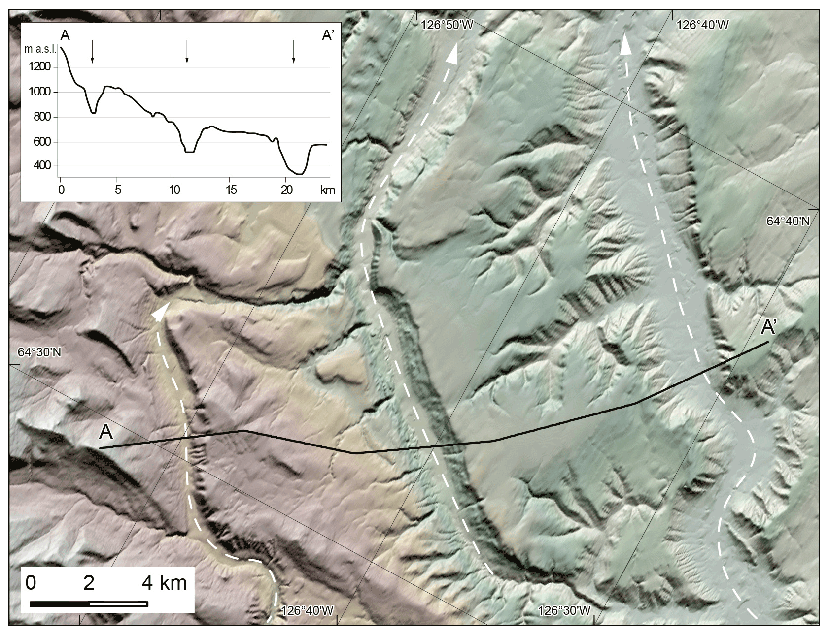
Figure 9A series of large marginal spillways along the eastern slopes of the Mackenzie Mountains. White dashed arrows indicate the meltwater flow direction. The location of this figure is indicated in Fig. 2.
Large marginal spillways incised along the eastern slopes of Mackenzie Mountains provide evidence for major melting in this part of the LIS (Fig. 9; Duk-Rodkin and Hughes, 1991; Lemmen et al., 1994; Bednarski, 2008). These meltwater channels are oriented parallel to the range front and drain to the north, located near the LGM limits of the NW LIS, and are located between the 14.9 and 14.2 ka ice margins of our reconstruction and so must have formed at this time (Fig. 4b and c). Thus, they do not record a long-term drainage of meltwater but rather high-magnitude discharge from the rapidly thinning NW LIS during early retreat.
We provide 30 new 10Be TCN constraints on the deglaciation of the NW LIS. Bayesian modelling of our TCN exposure ages indicates that the initial deglaciation of the NW LIS in the central Mackenzie Mountains began at ca. 15.8 ka (17.1–14.6 ka). The summits (∼1400 m) of the Franklin Mountains (∼63∘ N) deglaciated at ca. 14.9 ka (15.7–14.2 ka), with ice sheet surface lowering down to ∼800 m by ca. 14.3 ka (15.1–13.6 ka). The Norman Range (∼900 m) deglaciated at ca. 14.2 ka (15.0–13.6 ka), and the adjacent Mackenzie Valley (∼200 m) at 65∘ N deglaciated at ca. 13.6 ka (14.1–13.2 ka), opening the northern portion of the IFC. Our revised ice margin retreat chronology of the NW LIS accommodates the available age constraints on deglaciation, including our new TCN exposure ages. The main change in our reconstruction, compared with past work, is an earlier retreat of the NW LIS by about 1000 years around 63∘ N in the Mackenzie Mountains and Franklin Mountains. This results in broadly synchronous deglaciation of the Mackenzie Valley at 63 and 65∘ N, compared with past reconstructions which suggest that the region around 63∘ N deglaciated ∼1 ka later than the region to the north. According to our reconstruction, the IFC was not a viable migration route at the time of the peopling of North America around 14–15 ka. We find close agreement between our empirically based reconstruction and the sequence of events derived from the numerical ice sheet models of Gregoire et al. (2016). We use these model simulations to quantify the sea level contribution of the CIS–LIS saddle region during deglaciation, indicating a cumulative sea level contribution of 11.2 m from 16–13 ka.
The data referred to in this paper have all been provided within the tables and figures in the main text and in the Supplement. This includes the data input tables for recalculating our TCN exposure ages in the CRONUS online calculator (Balco et al., 2008). The supplementary materials related to this article are available in the Supplement and at https://doi.org/10.6084/m9.figshare.20069222.v3 (Stoker, 2022).
The supplement related to this article is available online at: https://doi.org/10.5194/tc-16-4865-2022-supplement.
The project was conceptualised by MM and DF with input from BJS and JMY. Cosmogenic nuclide samples were collected by MM, DF, BJS, and JMY. The laboratory processing and analysis of cosmogenic nuclide samples was undertaken by JCG and AJH. BJS curated the data used in this project and completed the analysis. The cosmogenic nuclide exposure age calculation approach was devised and undertaken by BJS under the supervision of MM and DF. The method to correct exposure ages for glacial isostatic adjustment was developed by SLN and MM and applied to the exposure ages by BJS. The Bayesian model setup was developed by AJM with input from JMY and discussions with BJS. The Bayesian model runs were performed by AJM. The ice sheet saddle collapse model was originally developed by LJG, and the model analysis presented in this paper was performed by NG. The manuscript was written by BJS and MM with input from all the authors. The data visualisation and figure creation was completed by BJS with input from all authors.
The contact author has declared that none of the authors has any competing interests.
Publisher's note: Copernicus Publications remains neutral with regard to jurisdictional claims in published maps and institutional affiliations.
We thank Guang Yang of the CRISDal lab at Dalhousie University for the cosmogenic nuclide sample preparation and chemistry. We are grateful for discussions with Jakub Heyman regarding the expage exposure age during the development of our GIA correction process; without these discussions the sensitivity analysis provided in the Supplement would not have been possible. The discussion and comments that arose during the revision stage from two anonymous reviewers and Pippa Whitehouse shaped the manuscript and helped increase the clarity of the paper. DEMs were provided by the Polar Geospatial Center under NSF-OPP awards 1043681, 1559691, and 1542736.
This research was supported by the Czech Science Foundation (grant no. 19-21216Y), the Swedish Research Council International Postdoctoral Fellowship (grant no. 637-2014-483) awarded to Martin Margold, the Charles University Grant Agency project (GAUK project no. 122220) awarded to Benjamin J. Stoker, grants from the NRCan Polar Continental Shelf Program and the Natural Science and Engineering Research Council awarded to Duane Froese, and grants from the University of Alberta Northern Research Awards awarded to Joseph M. Young.
This paper was edited by Pippa Whitehouse and reviewed by two anonymous referees.
Antevs, E.:. The spread of aboriginal man to North America, Geogr. Rev., 25, 302–309, https://doi.org/10.2307/209605, 1935.
Applegate, P. J. and Alley, R. B.: Challenges in the use of cosmogenic exposure dating of moraine boulders to trace the geographic extents of abrupt climate changes: the Younger Dryas example, Abrupt Climate Change: Mechanisms, Patterns, and Impacts, 193, 111–122, https://doi.org/10.1029/GM193, 2011.
Balco, G.: Contributions and unrealized potential contributions of cosmogenic-nuclide exposure dating to glacier chronology, 1990–2010, Quaternary Sci. Rev., 30, 3–27, https://doi.org/10.1016/j.quascirev.2010.11.003, 2011.
Balco, G.: Glacier change and paleoclimate applications of cosmogenic-nuclide exposure dating, Annu. Rev. Earth Planet. Sci., 48, 21–48, https://doi.org/10.1146/annurev-earth-081619-052609, 2020.
Balco, G., Stone, J. O., Lifton, N. A., and Dunai, T. J.: A complete and easily accessible means of calculating surface exposure ages or erosion rates from 10Be and 26Al measurements, Quaternary Geochronol., 3, 174–195, https://doi.org/10.1016/j.quageo.2007.12.001, 2008.
Barth, A. M., Marcott, S. A., Licciardi, J. M., and Shakun, J. D.: Deglacial thinning of the Laurentide Ice Sheet in the Adirondack Mountains, New York, USA, revealed by 36Cl exposure dating, Paleoceanogr. Paleocl., 34, 946–953, https://doi.org/10.1029/2018PA003477, 2019.
Bateman, M. D. and Murton, J. B.: The chronostratigraphy of Late Pleistocene glacial and periglacial aeolian activity in the Tuktoyaktuk Coastlands, NWT, Canada, Quaternary Sci. Rev., 25, 2552–2568, https://doi.org/10.1016/j.quascirev.2005.07.023, 2006.
Bednarski, J. M.: Landform assemblages produced by the Laurentide Ice Sheet in northeastern British Columbia and adjacent Northwest Territories – constraints on glacial lakes and patterns of ice retreat, Can. J. Earth Sci., 45, 593–610, https://doi.org/10.1139/E07-053, 2008.
Borchers, B., Marrero, S., Balco, G., Caffee, M., Goehring, B., Lifton, N., Nishiizumi, K., Phillips, F., Schaefer, J., and Stone, J.: Geological calibration of spallation production rates in the CRONUS-Earth project, Quaternary Geochronol., 31, 188–198, https://doi.org/10.1016/j.quageo.2015.01.009, 2016.
Braje, T. J., Dillehay, T. D., Erlandson, J. M., Klein, R. G., and Rick, T. C.: Finding the first Americans, Science, 358, 592–594, 2017.
Braje, T. J., Erlandson, J. M., Rick, T. C., Davis, L., Dillehay, T., Fedje, D. W., Froese, D., Gusick, A., Mackie, Q., McLaren, D., and Pitblado, B.: Fladmark+ 40: What have we learned about a potential Pacific Coast peopling of the Americas?, American Antiquity, 85, 1–21, https://doi.org/10.1017/aaq.2019.80, 2020.
Briner, J. P., Gosse, J. C., Bierman, P. R., and Siame, L. L.: Applications of cosmogenic nuclides to Laurentide Ice Sheet history and dynamics, Special Papers-Geol. Soc. Am., 415, 29, https://doi.org/10.1130/2006.2415(03), 2006.
Broecker, W. S., Kennett, J. P., Flower, B. P., Teller, J. T., Trumbore, S., Bonani, G., and Wolfli, W.: Routing of meltwater from the Laurentide Ice Sheet during the Younger Dryas cold episode, Nature, 341, 318–321, https://doi.org/10.1038/341318a0, 1989.
Bronk Ramsey, C.: Bayesian analysis of radiocarbon dates, Radiocarbon, 51, 337–360, https://doi.org/10.1017/S0033822200033865, 2009a.
Bronk Ramsey, C.: Dealing with outliers and offsets in radiocarbon dating, Radiocarbon, 51, 1023–1045, 2009b.
Bronk Ramsey, C.: OxCal 4.3, https://c14.arch.ox.ac.uk/oxcal/Oxcalhtml (last access: February 2022), 2017.
Buck, C. E., Cavanagh, W. G., Litton, C. D., and Scott, M.: Bayesian approach to interpreting archaeological data, Wiley, Chichester, 402, 1996.
Church, J. A., Clark, P. U., Cazenave, A., Gregory, J. M., Jevrejeva, S., Levermann, A., Merrifield, M. A., Milne, G. A., Nerem, R. S., Nunn, P. D., Payne, A. J., Pfeffer, W. T., Stammer, D., and Unnikrishnan, A. S.: Sea Level Change, in: Climate Change 2013: The Physical Science Basis. Contribution of Working Group I to the Fifth Assessment Report of the Intergovernmental Panel on Climate Change, edited by: Jouzel, J., van de Wal, R., Woodworth, P. L., and Xiao, C., Cambridge University Press, Cambridge, United Kingdom and New York, NY, USA, http://drs.nio.org/drs/handle/2264/4605, 2013.
Clark, J., Carlson, A. E., Reyes, A. V., Carlson, E. C., Guillaume, L., Milne, G. A., Tarasov, L., Caffee, M., Wilcken, K., and Rood, D. H.: The age of the opening of the Ice-Free Corridor and implications for the peopling of the Americas, P. Natl. Acad. Sci. USA, 119, e2118558119, https://doi.org/10.1073/pnas.2118558119, 2022.
Clark, P. U. and Mix, A. C.: Ice sheets and sea level of the Last Glacial Maximum, Quaternary Sci. Rev., 21, 1–7, https://doi.org/10.1016/S0277-3791(01)00118-4, 2002.
Clark, P. U., Marshall, S. J., Clarke, G. K., Hostetler, S. W., Licciardi, J. M., and Teller, J. T.: Freshwater forcing of abrupt climate change during the last glaciation, Science, 293, 283–287, 2001.
Condron, A. and Winsor, P.: Meltwater routing and the Younger Dryas, P. Natl. Acad. Sci. USA, 109, 19928–19933, 2012.
Corbett, L. B., Bierman, P. R., Wright, S. F., Shakun, J. D., Davis, P. T., Goehring, B. M., Halsted, C. T., Koester, A. J., Caffee, M. W., and Zimmerman, S. R.: Analysis of multiple cosmogenic nuclides constrains Laurentide Ice Sheet history and process on Mt. Mansfield, Vermont's highest peak, Quaternary Sci. Rev., 205, 234–246, 2019.
Cuzzone, J. K., Clark, P. U., Carlson, A. E., Ullman, D. J., Rinterknecht, V. R., Milne, G. A., Lunkka, J. P., Wohlfarth, B., Marcott, S. A., and Caffee, M.: Final deglaciation of the Scandinavian Ice Sheet and implications for the Holocene global sea-level budget, Earth Planet. Sc. Lett., 448, 34–41, 2016.
Dalton, A. S., Margold, M., Stokes, C. R., et al.: An updated radiocarbon-based ice margin chronology for the last deglaciation of the North American Ice Sheet Complex, Quaternary Sci. Rev., 234, 106223, https://doi.org/10.1016/j.quascirev.2020.106223, 2020.
Deschamps, P., Durand, N., Bard, E., Hamelin, B., Camoin, G., Thomas, A. L., Henderson, G. M., Okuno, J. i., and Yokoyama, Y.: Ice-sheet collapse and sea-level rise at the Bolling warming 14,600 years ago, Nature, 483, 559–564, 2012.
Duk-Rodkin, A. and Hughes, O.: Age relationships of Laurentide and montane glaciations, Mackenzie Mountains, Northwest Territories, Géographie physique et Quaternaire, 45, 79–90, 1991.
Duk-Rodkin, A., Barendregt, R. W., Tarnocai, C., and Phillips, F. M.: Late Tertiary to late Quaternary record in the Mackenzie Mountains, Northwest Territories, Canada: stratigraphy, paleosols, paleomagnetism, and chlorine – 36, Can. J. Earth Sci., 33, 875–895, https://doi.org/10.1139/e96-066, 1996.
Dulfer, H. E., Margold, M., Engel, Z., Braucher, R., and Team, A.: Using 10Be dating to determine when the Cordilleran Ice Sheet stopped flowing over the Canadian Rocky Mountains, Quaternary Res., 102, 1–12, https://doi.org/10.1017/qua.2020.122, 2021.
Dunai, T. J.: Cosmogenic nuclides: principles, concepts and applications in the earth surface sciences, Cambridge University Press, https://doi.org/10.1017/CBO9780511804519, 2010.
Dyke, A. S., Andrews, J. T., Clark, P. U., England, J. H., Miller, G. H., Shaw, J., and Veillette, J. J.: The Laurentide and Innuitian ice sheets during the Last Glacial Maximum, Quaternary Sci. Rev., 21, 9–31, https://doi.org/10.1016/S0277-3791(01)00095-6, 2002.
Dyke, A. S., Moore, A., and Robertson, L.: Deglaciation of North America. Geological Survey of Canada, Open File 1574, Ottawa, 2003.
Fisher, T. G., Yansa, C. H., Lowell, T. V., Lepper, K., Hajdas, I., and Ashworth, A.: The chronology, climate, and confusion of the Moorhead Phase of glacial Lake Agassiz: new results from the Ojata Beach, North Dakota, USA, Quaternary Sci. Rev., 27, 1124–1135, 2008.
Fladmark, K. R.: Routes: Alternate migration corridors for early man in North America, American Antiquity, 44, 55–69, 1979.
Froese, D. G., Young, J. M., Norris, S. L., and Margold, M.: Availability and viability of the ice-free corridor and Pacific coast routes for the peopling of the Americas, The SAA [Society for American Archaeology] Archaeological Record, 19, 27–33, 2019.
Goebel, T., Waters, M. R., and O'Rourke, D. H.: The late Pleistocene dispersal of modern humans in the Americas, Science, 319, 1497–1502, 2008.
Gomez, N., Gregoire, L. J., Mitrovica, J. X., and Payne, A. J.: Laurentide-Cordilleran Ice Sheet saddle collapse as a contribution to meltwater pulse 1A, Geophys. Res. Lett., 42, 3954–3962, 2015.
Gosse, J. C. and Phillips, F. M.: Terrestrial in situ cosmogenic nuclides: theory and application, Quaternary Sci. Rev., 20, 1475–1560, 2001.
Government of Canada: Canadian Climate Normals 1981–2010, Station for Norman Wells and Fort Simpson, http://climate.weather.gc.ca/climate_normals/results_1981_2010_e.html?searchType=stnProv&lstProvince=NT&stnID=1656, last access: 26 March 2019.
Gowan, E. J.: An assessment of the minimum timing of ice free conditions of the western Laurentide Ice Sheet, Quaternary Sci. Rev., 75, 100–113, 2013.
Gowan, E. J., Tregoning, P., Purcell, A., Montillet, J. P., and McClusky, S.: A model of the western Laurentide Ice Sheet, using observations of glacial isostatic adjustment, Quaternary Sci. Rev., 139, 1–16, 2016.
Gowan, E. J., Zhang, X., Khosravi, S., Rovere, A., Stocchi, P., Hughes, A. L., Gyllencreutz, R., Mangerud, J., Svendsen, J. I., and Lohmann, G.: A new global ice sheet reconstruction for the past 80 000 years, Nat. Commun., 12, 1–9, 2021.
Gregoire, L. J., Payne, A. J., and Valdes, P. J.: Deglacial rapid sea level rises caused by ice-sheet saddle collapses, Nature, 487, 219–222, 2012.
Gregoire, L. J., Valdes, P. J., and Payne, A. J.: The relative contribution of orbital forcing and greenhouse gases to the North American deglaciation, Geophys. Res. Lett., 42, 2015GL066005, https://doi.org/10.1002/2015GL066005, 2015.
Gregoire, L. J., Otto-Bliesner, B., Valdes, P. J., and Ivanovic, R.: Abrupt Bølling warming and ice saddle collapse contributions to the Meltwater Pulse 1a rapid sea level rise, Geophys. Res. Lett., 43, 9130–9137, 2016.
Heintzman, P. D., Froese, D., Ives, J. W., Soares, A. E., Zazula, G. D., Letts, B., Andrews, T. D., Driver, J. C., Hall, E., Hare, P. G., and Jass, C. N.: Bison phylogeography constrains dispersal and viability of the Ice Free Corridor in western Canada, P. Natl. Acad. Sci. USA, 113, 8057–8063, 2016.
Heyman, J.: Expage global compilation of cosmogenic exposure ages, https://expage.github.io/data.html, last access: 10 February 2022.
Heyman, J., Applegate, P. J., Blomdin, R., Gribenski, N., Harbor, J. M., and Stroeven, A. P.: Boulder height–exposure age relationships from a global glacial 10Be compilation, Quaternary Geochronol., 34, 1–11, 2016.
Heyman, J., Stroeven, A. P., Harbor, J. M., and Caffee, M. W.: Too young or too old: evaluating cosmogenic exposure dating based on an analysis of compiled boulder exposure ages, Earth Planet. Sc. Lett., 302, 71–80, 2011.
Ivanovic, R. F., Gregoire, L. J., Wickert, A. D., Valdes, P. J., and Burke, A.: Collapse of the North American ice saddle 14,500 years ago caused widespread cooling and reduced ocean overturning circulation, Geophys. Res. Lett., 44, 383–392, 2017.
Ives, J. W., Froese, D., Supernant, K., and Yanicki, G.: Vectors, vestiges and Valhallas: Rethinking the corridor, in: Paleoamerican Odyssey, edited by: Graf, K. E., Ketron, C. V., and Waters, M. R., Texas A&M University Press, College Station, 149–169, 2013.
Jackson Jr., L. E., Phillips, F. M., Shimamura, K., and Little, E. C.: Cosmogenic 36Cl dating of the Foothills erratics train, Alberta, Canada, Geology, 25, 195–198, 1997.
Johnston, W. A.: Quaternary geology of North America in relation to the migration of man, in: The American Aborigines, edited by: Jenness, D., 11–45, 1933.
Jones, R. S., Mackintosh, A. N., Norton, K. P., Golledge, N. R., Fogwill, C. J., Kubík, P. W., Christl, M., and Greenwood, S. L.: Rapid Holocene thinning of an East Antarctic outlet glacier driven by marine ice sheet instability, Nat. Commun., 6, 8910, https://doi.org/10.1038/ncomms9910, 2015.
Jones, R. S., Whitehouse, P. L., Bentley, M. J., Small, D., and Dalton, A. S.: Impact of glacial isostatic adjustment on cosmogenic surface-exposure dating, Quaternary Sci. Rev., 212, 206–212, 2019.
Keigwin, L. D., Klotsko, S., Zhao, N., Reilly, B., Giosan, L., and Driscoll, N. W.: Deglacial floods in the Beaufort Sea preceded Younger Dryas cooling, Nat. Geosci., 11, 599–604, https://doi.org/10.1038/s41561-018-0169-6, 2018.
Kennedy, K. E., Froese, D. G., Zazula, G. D., and Lauriol, B.: Last Glacial Maximum age for the northwest Laurentide maximum from the Eagle River spillway and delta complex, northern Yukon, Quaternary Sci. Rev., 29, 1288–1300, 2010.
Koester, A. J., Shakun, J. D., Bierman, P. R., Davis, P. T., Corbett, L. B., Braun, D., and Zimmerman, S. R.: Rapid thinning of the Laurentide Ice Sheet in coastal Maine, USA, during late Heinrich Stadial 1, Quaternary Sci. Rev., 163, 180–192, 2017.
Koester, A. J., Shakun, J. D., Bierman, P. R., Davis, P. T., Corbett, L. B., Goehring, B. M., Vickers, A. C., and Zimmerman, S. R.: Laurentide ice sheet thinning and erosive regimes at Mount Washington, New Hampshire, inferred from multiple cosmogenic nuclides, in: Untangling the Quaternary Period – A Legacy of Stephen C. Porter, edited by: Waitt, R. B., Thackray, G. D., and Gillespie, A. R., Geological Society of America, Boulder, Colorado, USA, 548, https://doi.org/10.1130/2020.2548(15), 2021.
Kohl, C. P. and Nishiizumi, K.: Chemical isolation of quartz for measurement of in-situ -produced cosmogenic nuclides, Geochim. Cosmochim. Ac., 56, 3583–3587, 1992.
Lacelle, D., Lauriol, B., Zazula, G., Ghaleb, B., Utting, N., and Clark, I. D.: Timing of advance and basal condition of the Laurentide Ice Sheet during the last glacial maximum in the Richardson Mountains, NWT, Quaternary Res., 80, 274–283, 2013.
Lal, D.: Cosmic ray labeling of erosion surfaces: in situ nuclide production rates and erosion models, Earth Planet. Sc. Lett., 104, 424–439, 1991.
Lambeck, K., Purcell, A., and Zhao, S.: The North American Late Wisconsin ice sheet and mantle viscosity from glacial rebound analyses, Quaternary Sci. Rev., 158, 172–210, 2017.
Lemmen, D. S., Duk-Rodkin, A., and Bednarski, J. M.: Late glacial drainage systems along the northwestern margin of the Laurentide Ice Sheet, Quaternary Sci. Rev., 13, 805–828, 1994.
Lesnek, A. J., Briner, J. P., Lindqvist, C., Baichtal, J. F., and Heaton, T. H.: Deglaciation of the Pacific coastal corridor directly preceded the human colonization of the Americas, Sci. Adv., 4, 1528–1531, 2018.
Licciardi, J. M., Clark, P. U., Jenson, J. W., and MacAyeal, D. R.: Deglaciation of a soft-bed Laurentide Ice Sheet, Quaternary Sci. Rev., 17, 427–448, 1998.
Lin, Y., Hibbert, F. D., Whitehouse, P. L., Woodroffe, S. A., Purcell, A., Shennan, I., and Bradley, S. L.: A reconciled solution of Meltwater Pulse 1A sources using sea-level fingerprinting, Nat. Commun., 12, 1–11, 2021.
Liu, J., Milne, G. A., Kopp, R. E., Clark, P. U., and Shennan, I.: Sea-level constraints on the amplitude and source distribution of Meltwater Pulse 1A, Nat. Geosci., 9, 130–134, 2016.
Mandryk, C. A.: Late Wisconsinan deglaciation of Alberta: Processes and paleogeography, Quaternary Int., 32, 79–85, 1996.
Margold, M., Gosse, J. C., Hidy, A. J., Woywitka, R. J., Young, J. M., and Froese, D.: Beryllium-10 dating of the Foothills Erratics Train in Alberta, Canada, indicates detachment of the Laurentide Ice Sheet from the Rocky Mountains at ∼15 ka, Quaternary Res., 92, 469–482, 2019.
Mas e Braga, M., Selwyn Jones, R., Newall, J. C. H., Rogozhina, I., Andersen, J. L., Lifton, N. A., and Stroeven, A. P.: Nunataks as barriers to ice flow: implications for palaeo ice sheet reconstructions, The Cryosphere, 15, 4929–4947, https://doi.org/10.5194/tc-15-4929-2021, 2021.
Meachen, J. A., Brannick, A. L., and Fry, T. J.: Extinct Beringian wolf morphotype found in the continental US has implications for wolf migration and evolution, Ecol. Evol., 6, 3430–3438, 2016.
Menounos, B., Goehring, B. M., Osborn, G., Margold, M., Ward, B., Bond, J., Clarke, G. K., Clague, J. J., Lakeman, T., Koch, J., and Caffee, M. W.: Cordilleran Ice Sheet mass loss preceded climate reversals near the Pleistocene Termination, Science, 358, 781–784, 2017.
Mitchell, K. J., Bover, P., Salis, A. T., Mudge, C., Heiniger, H., Thompson, M., Hockett, B., Weyrich, L.S., Cooper, A., and Meachen, J. A.: Evidence for Pleistocene gene flow through the ice-free corridor from extinct horses and camels from Natural Trap Cave, Wyoming, Quaternary International, https://doi.org/10.1016/j.quaint.2021.11.017, 2021.
Munyikwa, K., Feathers, J. K., Rittenour, T. M., and Shrimpton, H. K.: Constraining the Late Wisconsinan retreat of the Laurentide ice sheet from western Canada using luminescence ages from postglacial aeolian dunes, Quaternary Geochronol., 6, 407–422, 2011.
Murton, J. B., Frechen, M., and Maddy, D.: Luminescence dating of mid-to Late Wisconsinan aeolian sand as a constraint on the last advance of the Laurentide Ice Sheet across the Tuktoyaktuk Coastlands, western Arctic Canada, Can. J. Earth Sci., 44, 857–869, 2007.
Murton, J. B., Bateman, M. D., Dallimore, S. R., Teller, J. T., and Yang, Z.: Identification of Younger Dryas outburst flood path from Lake Agassiz to the Arctic Ocean, Nature, 464, 740–743, 2010.
Murton, J. B., Bateman, M. D., Waller, R. I., and Whiteman, C. A.: September. Late Wisconsin glaciation of Hadwen and Summer islands, Tuktoyaktuk Coastlands, NWT, Canada, GEOQuébec2015, 7th Canadian Permafrost Conference, pp. 20–23, 2015.
Nishiizumi, K., Imamura, M., Caffee, M. W., Southon, J. R., Finkel, R. C., and McAninch, J.: Absolute calibration of 10Be AMS standards: Nuclear Instruments and Methods, Phys. Res. Sect. B, 258, 403–413, 2007.
Norris, S., Tarasov, L., Monteath, A. J., Gosse, J. C., Hidy, A. J., Margold, M., and Froese, D. G.: Rapid retreat of the southwestern Laurentide Ice Sheet during the Bølling-Allerød interval, Geology, 50, 417–421, https://doi.org/10.1130/G49493.1, 2022.
Norris, S. L., Garcia-Castellanos, D., Jansen, J. D., Carling, P. A., Margold, M., Woywitka, R. J., and Froese, D. G.: Catastrophic drainage from the northwestern outlet of glacial Lake Agassiz during the Younger Dryas, Geophys. Res. Lett., 48, e2021GL093919, https://doi.org/10.1029/2021GL093919, 2021.
Pedersen, M. W., Ruter, A., Schweger, C., Friebe, H., Staff, R. A., Kjeldsen, K. K., Mendoza, M. L., Beaudoin, A. B., Zutter, C., Larsen, N. K., and Potter, B. A.: Postglacial viability and colonization in North America's ice-free corridor, Nature, 537, 45–49, 2016.
Peltier, W. R., Argus, D. F., and Drummond, R.: Space geodesy constrains ice age terminal deglaciation: The global ICE-6G_C (VM5a) model, J. Geophys. Res.-Sol. Ea., 120, 450–487, 2015.
Pendleton, S., Condron, A., and Donnelly, J.: The potential of Hudson Valley glacial floods to drive abrupt climate change, Commun. Earth Environ., 2, 1–7, 2021.
Plug, L. J., Gosse, J. C., McIntosh, J. J., and Bigley, R.: Attenuation of cosmic ray flux in temperate forest, J. Geophys. Res.-Earth Surf., 112, F02022, https://doi.org/10.1029/2006JF000668, 2007.
Porter, C., Morin, P., Howat, I., Noh, M.-J., Bates, B., Peterman, K., Keesey, S., Schlenk, M., Gardiner, J., Tomko, K., Willis, M., Kelleher, C., Cloutier, M., Husby, E., Foga, S., Nakamura, H., Platson, M., Wethington Jr., M., Williamson, C., Bauer, G., Enos, J., Arnold, G., Kramer, W., Becker, P., Doshi, A., D'Souza, C., Cummens, P., Laurier, F., and Bojesen, M.: “ArcticDEM”, Harvard Dataverse, V1, https://doi.org/10.7910/DVN/OHHUKH, 2018.
Potter, B. A., Baichtal, J. F., Beaudoin, A. B., Fehren-Schmitz, L., Haynes, C. V., Holliday, V. T., Holmes, C. E., Ives, J. W., Kelly, R. L., Llamas, B., and Malhi, R. S.: Current evidence allows multiple models for the peopling of the Americas, Sci. Adv., 4, eaat5473, https://doi.org/10.1126/sciadv.aat547, 2018.
Reimer, P. J., Austin, W. E., Bard, E., Bayliss, A., Blackwell, P. G., Ramsey, C. B., Butzin, M., Cheng, H., Edwards, R. L., Friedrich, M., and Grootes, P. M.: The IntCal20 Northern Hemisphere radiocarbon age calibration curve (0–55 cal kBP), Radiocarbon, 62, 725–757, 2020.
Reyes, A. V., Carlson, A. E., Milne, G. A., Tarasov, L., Reimink, J. R., and Caffee, M. W.: Revised chronology of northwest Laurentide ice-sheet deglaciation from 10Be exposure ages on boulder erratics, Quaternary Sci. Rev., 277, 107369, https://doi.org/10.1016/j.quascirev.2021.107369, 2022.
Simms, A. R., Lisiecki, L., Gebbie, G., Whitehouse, P. L., and Clark, J. F.: Balancing the last glacial maximum (LGM) sea-level budget, Quaternary Sci. Rev., 205, 143–153, 2019.
Small, D., Bentley, M. J., Jones, R. S., Pittard, M. L., and Whitehouse, P. L.: Antarctic ice sheet palaeo-thinning rates from vertical transects of cosmogenic exposure ages, Quaternary Sci. Rev., 206, 65–80, 2019.
Smith, D. G.: Glacial Lake Mackenzie, Mackenzie Valley, Northwest Territories, Canada, Can. J. Earth Sci., 29, 1756–1766, https://doi.org/10.1139/e92-138, 1992.
Smith, D. G.: Glacial Lake McConnell: paleogeography, age, duration, and associated river deltas, Mackenzie River basin, western Canada, Quaternary Sci. Rev., 13, 829–843, 1994.
Smith, D. G. and Fisher, T. G.: Glacial Lake Agassiz: The northwestern outlet and paleoflood, Geology, 21, 9–12, https://doi.org/10.1130/0091-7613(1993)021<0009:GLATNO>2.3.CO;2, 1993.
Staiger, J., Gosse, J., Toracinta, R., Oglesby, B., Fastook, J., and Johnson, J. V.: Atmospheric scaling of cosmogenic nuclide production: climate effect, J. Geophys. Res.-Sol. Ea., 112, B02205, https://doi.org/10.1029/2005JB003811, 2007.
Stoker, B. J.: The collapse of the Laurentide-Cordilleran ice saddle and early opening of the Mackenzie Valley, Northwest Territories, constrained by 10Be exposure dating – supplementary materials, figshare [data set], https://doi.org/10.6084/m9.figshare.20069222.v3, 2022.
Stone, J. O.: Air pressure and cosmogenic isotope production, J. Geophys. Res.-Sol. Ea., 105, 23753–23759, 2000.
Stuiver, M., Reimer, P. J., and Reimer, R. W.: CALIB 8.2, http://calib.org, last access: 20 December 2021.
Tarasov, L., Dyke, A. S., Neal, R. M., and Peltier, W. R.: A data-calibrated distribution of deglacial chronologies for the North American ice complex from glaciological modeling, Earth Planet. Sc. Lett., 315, 30–40, 2012.
Teller, J. T., Leverington, D. W., and Mann, J. D.: Freshwater outbursts to the oceans from glacial Lake Agassiz and their role in climate change during the last deglaciation, Quaternary Sci. Rev., 21, 879–887, 2002.
Teller, J. T., Boyd, M., Yang, Z., Kor, P. S., and Fard, A. M.: Alternative routing of Lake Agassiz overflow during the Younger Dryas: new dates, paleotopography, and a re-evaluation, Quaternary Sci. Rev., 24, 1890–1905, 2005.
Ullman, D. J., Carlson, A. E., Hostetler, S. W., Clark, P. U., Cuzzone, J., Milne, G. A., Winsor, K., and Caffee, M.: Final Laurentide ice-sheet deglaciation and Holocene climate-sea level change, Quaternary Sci. Rev., 152, 49–59, 2016.
Waters, M. R.: Late Pleistocene exploration and settlement of the Americas by modern humans, Science, 365, eaat5447, https://doi.org/10.1126/science.aat5447, 2019.
Wolfe, S., Huntley, D., and Ollerhead, J.: Relict late Wisconsinan dune fields of the northern Great Plains, Canada, Géographie physique et Quaternaire, 58, 323–336, 2004.
Wolfe, S. A., Ollerhead, J., Huntley, D. J., and Lian, O. B.: Holocene dune activity and environmental change in the prairie parki and and boreal forest, central Saskatchewan, Canada, Holocene, 16, 17–29, 2006.
Wolfe, S. A., Paulen, R. C., Smith, I. R., and Lamothe, M.: Age and paleoenvironmental significance of Late Wisconsinan dune fields in the Mount Watt and Fontas River map areas, northern Alberta and British Columbia, Geological Survey of Canada, Current Research, 2007-B4, 10, 2007.
Young, J. M., Reyes, A. V., and Froese, D. G.: Assessing the ages of the Moorhead and Emerson phases of glacial Lake Agassiz and their temporal connection to the Younger Dryas cold reversal, Quaternary Sci. Rev., 251, 106714, https://doi.org/10.1016/j.quascirev.2020.106714, 2021.
Young, N. E., Schaefer, J. M., Briner, J. P., and Goehring, B. M.: A 10Be production-rate calibration for the Arctic, J. Quaternary Sci., 28, 515–526, 2013.