Predicting the steady-state isochronal stratigraphy of ice shelves using observations and modeling

Ice shelves surrounding the Antarctic perimeter moderate ice discharge towards the ocean through buttressing. Ice-shelf evolution and integrity depend on the local surface accumulation, basal melting and on the spatially variable ice-shelf viscosity. These components of ice-shelf mass balance are often poorly constrained by observations and introduce uncertainties in ice-sheet projections. Isochronal radar stratigraphy is an observational archive for the atmospheric, oceanographic and ice-flow history of ice shelves. Here, we predict the stratigraphy of locally accumulated ice on ice shelves with a kinematic forward model for a given atmospheric and oceanographic scenario. This delineates the boundary between local meteoric ice (LMI) and continental meteoric ice (CMI). A large LMI to CMI ratio hereby marks ice shelves whose buttressing strength is more sensitive to changes in atmospheric precipitation patterns. A mismatch between the steady-state predictions of the kinematic forward model and observations from radar can highlight inconsistencies in the atmospheric and oceanographic input data or be an indicator for a transient ice-shelf history not accounted for in the model. We discuss pitfalls in numerical diffusion when calculating the age field and validate the kinematic model with the full Stokes ice-flow model Elmer/Ice. The Roi Baudouin Ice Shelf (East Antarctica) serves as a test case for this approach. There, we find a significant east–west gradient in the LMI / CMI ratio. The steady-state predictions concur with observations on larger spatial scales (>10 km), but deviations on smaller scales are significant, e.g., because local surface accumulation patterns near the grounding zone are underestimated in Antarctic-wide estimates. Future studies can use these mismatches to optimize the input data or to pinpoint transient signatures in the ice-shelf history using the ever growing archive of radar observations of internal ice stratigraphy.

1 Introduction

The Antarctic Ice Sheet holds a sea level equivalent ice volume of ca. 58 m of global sea level rise (Fretwell et al., 2013; Morlighem et al., 2020), with maximum estimates of up to 40 cm by the end of this century (Levermann et al., 2020; Edwards et al., 2021). Forming at the outlets of the ice–ocean boundary surrounding Antarctica, ice shelves play a major role in these future projections due to their buttressing effect on glacier flow (Fürst et al., 2016). The stability of ice shelves has been a focus of many studies (Rignot et al., 2008; Jansen et al., 2010; Gudmundsson, 2013; Alley et al., 2016; Fürst et al., 2016; Banwell, 2017; Schannwell et al., 2018), and predicting their future behavior requires understanding the impact of future changes in atmospheric and oceanic forcing on their structural integrity. Uncertainties in ice-shelf evolution are in part due to an insufficient understanding of the processes which drive ocean-induced melting at the grounding-line and further seawards. The internal ice-shelf stratigraphy, as imaged by radar, is an underexplored archive which can be used to better constrain model predictions.

In grounded ice, numerous localized studies have used radar observations to infer surface and basal accumulation history (Nereson et al., 1998, 2000; Nereson and Waddington, 2002; Waddington et al., 2007; Hindmarsh et al., 2009; Catania et al., 2010; Leysinger Vieli et al., 2011; Lenaerts et al., 2014; Jenkins, 2016; Holschuh et al., 2017; Lenaerts et al., 2019; Pratap et al., 2021) of various sectors in Greenland or Antarctica. These approaches also gave insights into dynamic processes, e.g., such as basal sliding (Holschuh et al., 2017) and englacial folding (Bons et al., 2016; Jansen et al., 2016). Recent studies have focused on using the geometry of isochronal radar reflection horizons to reconstruct the ice dynamics of mountain glaciers (Jouvet et al., 2020) and also on a continental scale in Greenland (Born and Robinson, 2021) and Antarctica (Sutter et al., 2021). In ice shelves, similar concepts have been applied to derive the surface accumulation (e.g., Pratap et al., 2021) and basal melt rates (Pattyn et al., 2012a; Matsuoka et al., 2012; Das et al., 2020). The internal radar stratigraphy also holds information with respect to the ice shelf's dynamic history and internal structure (Das et al., 2020), but this has been less often exploited so far.

Here, we predict the age stratigraphy of locally accumulated ice on ice shelves for a given set of oceanic and atmospheric boundary conditions. The meteoric ice originating from the grounded part of the ice sheet is overlaid by the ice originating from local accumulation on the ice shelf. Consistent with previous publications (Das et al., 2020), we refer to these two ice bodies as local meteoric ice (LMI) and continental meteoric ice (CMI). The implications of the LMI / CMI ratio of a particular ice shelf are twofold. First, the two ice bodies can have different rheological properties because CMI, deposited further upstream, may contain colder and stiffer ice that protrudes into the ice shelves from their tributary ice streams (Larour et al., 2005; Khazendar et al., 2011). This ice may also show stronger orientation fabric because of stress–strain configurations experienced during flow (e.g., Alley, 1992; Thomas et al., 2021), whereas the LMI will not. Second, ice shelves that contain a large fraction of LMI are more susceptible to changes in atmospheric precipitation compared to ice shelves which are predominantly sustained by their tributary ice streams. This is relevant for future ice-shelf stability because some predictions suggest a stable or even decreasing surface accumulation for ice shelves in contrast to the overall predicted increase for the rest of the Antarctic continent (Kittel et al., 2021). In the following, we present details about the kinematic forward model (Sect. 2.1) and its validation (Sect. 2.2) including numerical uncertainties (Sect. 2.3). We then model the steady-state LMI stratigraphy of the Roi Baudouin Ice Shelf and compare the predictions with radar observations (Sect. 2.4). We interpret differences between observations and predictions in terms of flawed input data (oceanic, climatic) and/or transient signatures.

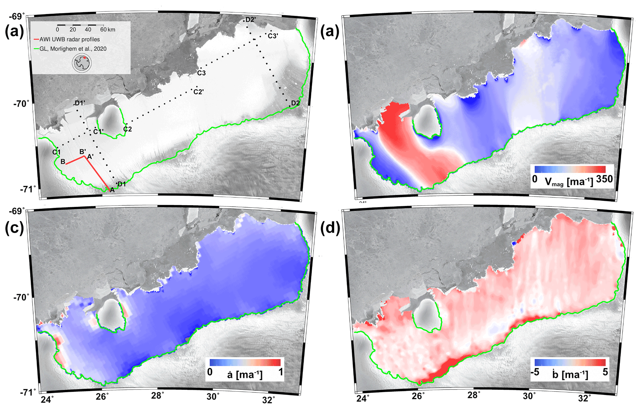
Figure 1 (a) Overview of the Roi Baudouin Ice Shelf located in Dronning Maud Land, East Antarctica. The grounding line (Morlighem et al., 2020) is marked in green, and radar profile lines, A–A^′ and B–B^′, used for validation are located in red. Dotted black lines C1, C2, C3, D1 and D2 correspond to the profiles shown in Figs. 5 and 6. The RADARSAT mosaic (Jezek, 2003) is shown in the background. (b) Surface speed (Gardner et al., 2018, 2019), (c) surface accumulation rate (positive for mass gain, Lenaerts et al., 2014) and (d) basal melt rates (positive for mass loss, Adusumilli et al., 2020).

2 Methods

The governing equation to predict the ice stratigraphy is the advective age equation:

$$\begin{array}{}\text{(1)}& {\displaystyle \frac{\partial A}{\partial t}}+\mathit{v}\cdot \mathrm{\nabla }A=\mathrm{1}.\end{array}$$

The age of ice A at depth z is given by aging (i.e., the source term on the right-hand side) and ice advection, where v is the ice velocity $(V_x,V_y,V_z)$. Contours of the age field provide a natural comparison to the isochronal radar observations. In the following, we derive the required 3D velocities from the surface velocities assuming plug flow (i.e., the shallow shelf assumption (SSA); Morland, 1987; MacAyeal, 1989; Weis et al., 1999; Sect. 2.1). We validate this assumption using the full Stokes model Elmer/Ice in a synthetic geometry (referred to as MISMIP EXP1 originating from the setup from Pattyn et al., 2012b; Sect. 2.2). Numerical diffusion in the solution of Eq. (1) is quantified with another test case (referred to as NumDiff experiment) where an analytical solution exists (Sect. 2.3). We then apply this method to the Roi Baudouin Ice Shelf (referred to as RBIS experiment) where radar data are available.

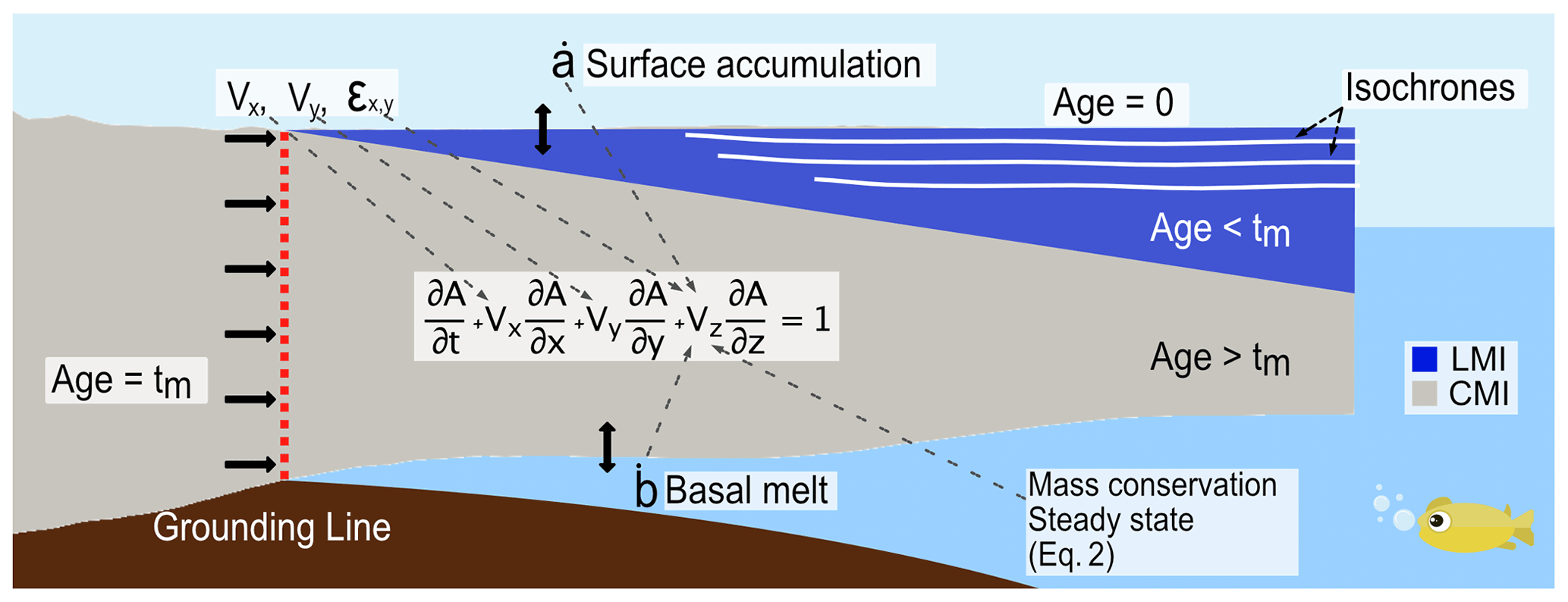
Figure 2 Illustration of the idealized ice shelf representing the distinction between the local meteoric ice (LMI, blue) and the continental meteoric ice advected from the ice sheet (CMI, gray). Isochrones are calculated by solving Eq. (1), using observed horizontal velocities (V_x, V_y) and derived vertical velocities including fixed surface accumulation and basal melt-rate fields (Eq. 2). On the inflow boundary upstream of the grounding line the age of ice is set to the length of the simulation time (t_m).

2.1 Prediction of ice-shelf stratigraphy with observed surface velocities

Vertical ice-flow velocities are derived from observed surface velocities (Drews et al., 2020) ice thickness H, the surface strain rates, the surface accumulation rate ($\dot{a}$, positive for mass gain), and the basal melt rate ($\dot{b}$, positive for mass loss):

$$\begin{array}{}\text{(2)}& V_z={\displaystyle \frac{{\mathit{\rho }}_{\mathrm{i}}}{{\mathit{\rho }}_{\mathrm{w}}}}\dot{a}+\left(\mathrm{1}-{\displaystyle \frac{{\mathit{\rho }}_{\mathrm{i}}}{{\mathit{\rho }}_{\mathrm{w}}}}\right)\dot{b}+\left[H\left(\mathrm{1}-{\displaystyle \frac{{\mathit{\rho }}_{\mathrm{i}}}{{\mathit{\rho }}_{\mathrm{w}}}}\right)+z\right]\mathrm{\nabla }\cdot {\mathit{V}}_{\mathrm{H}},\end{array}$$

where ρ_i and ρ_w are the respective densities of ice and water, and V_H is a vector containing horizontal surface velocities. We adopt a coordinate system such that z=0 corresponds to the ice surface, and z increases with depth. The x and y directions correspond to the along- and across-flow direction, respectively. The horizontal velocities at the surface (V_x,V_y) are obtained from observations, and it is assumed that they do not change with depth (i.e. plug flow), which is very well justified for ice shelves. With the 3D velocity field at hand, Eq. (1) is solved numerically using the open-source finite element library Elmer/Ice (Gagliardini et al., 2013). Velocity gradients are calculated using the strain rate solver in Elmer, and a separate solver is written to pass the vertical velocities from Eq. (2) to the age solver.

The age solver solves Eq. (1) with a semi-Lagrangian scheme (Martín and Gudmundsson, 2012). We set A(z=0) = 0, assuming that there is no ablation at the ice surface (Fig. 2). Due to a lack of observational age constraints at the grounding line, the age is initialized with 0 seawards of the grounding line. Upstream thereof, the age is initialized with the total runtime of the experiment, t_m. These initial conditions provide an easy way to delineate the CMI–LMI boundary by finding the line A=t_m. These boundary conditions lead to a kink in the age–depth profiles at the contact point between LMI and CMI. This cannot adequately be captured with the semi-Lagrangian tracing scheme, and deviations from the analytical and numerical schemes will be particularly evident around this transition (Sect. 3.2).

The results are verified by comparing the predicted isochrone stratigraphy with radar-observed internal layering (A–A^′, B–B^′; Fig. 1). The age of radar isochrones is often unknown, and consequently we can only compare spatial patterns and not absolute magnitudes. For the comparison of model results and observations, we contour the modeled age–depth field and choose a predicted isochrone with the same mean depth as the observed one (e.g., Nereson et al., 1998). Post-processing of the modeled age fields is done in Paraview (Henderson et al., 2004).

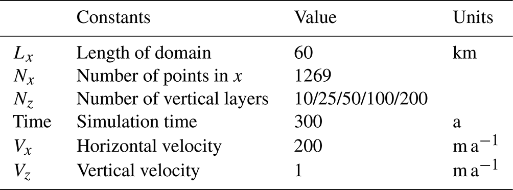
Steady-state conditions are assumed throughout. For the real-world test case scenario of the Roi Baudouin Ice Shelf (referred to as RBIS experiment), the ice-shelf geometry is obtained from BedMachine Antarctica (Morlighem et al., 2020), horizontal surface velocities are taken from satellite observations (Gardner et al., 2018, 2019), the surface accumulation rate is from RACMO 3.5 (Lenaerts et al., 2014), and the basal melt rate is from a compilation of satellite-derived surface height and velocity data combined with a firn layer model (Adusumilli et al., 2020). Those pan-Antarctic input data sets were chosen to enable an expansion of the applied methodology to all Antarctic ice shelves at a later stage. We run the simulations for 500 years, with 100 vertical layers, a horizontal resolution of 1 km and a time step of 0.1 year. The computation time (wall clock time) for a single simulation using 100 CPUs (central processing units) on five nodes is 22 h on a cluster with Intel Xeon E5-2630 processors. Prior to the real-world test case scenario we first validate the kinematic velocities and quantify numerical diffusion. Both are done for the cases with synthetic geometries.

2.2 Validation of derived velocities

Because Eq. (2) only holds in areas where the shallow-shelf assumption is valid, the validity of the analytical formula is tested in a synthetic experiment with an isothermal, isotropic, 2D, full Stokes model implemented in Elmer/Ice (Gagliardini et al., 2013). The model setup strictly follows the geometry and parameters used in the MISMIP EXP 1 experiment in the marine ice-sheet modeling intercomparison project (Pattyn et al., 2012b), with the exception of a reduced ice-shelf length (500 km), $\dot{a}=\mathrm{0.3}$ m a⁻¹ and $\dot{b}=\mathrm{0}$ m a⁻¹ (assuming a constant density of 917 kg m⁻³), and the grounding line condition is set to first floating (Gagliardini et al., 2013). The model is initialized close to a steady-state geometry from the EXP1 experiment (Pattyn et al., 2012b) and evolves to a steady state over 2500 years. A total of 20 vertical layers are used (corresponding to a mean spacing of around 20 m) and linearly increasing element spacing in the horizontal, ranging from less than 10 m near the grounding line up to 10 km towards the terminus. The modeled horizontal velocities are then used to derive vertical velocities using Eq. (2) and are compared to the full-Stokes vertical velocity calculated by Elmer/Ice. This comparison naturally highlights areas such as the grounding zone where the SSA assumptions of depth-invariable horizontal flow are violated, and the differences compared to the full-Stokes solution are the largest.

2.3 Quantification of numerical diffusion

In order to quantify numerical diffusion, we consider another time-invariant, unbuttressed, 2D slab of ice with constant and depth-invariant horizontal velocities (Fig. 4). Consequently the vertical velocities are also constant, and the trajectory along the LMI–CMI boundary z_DL(x) of a particle deposited at the grounding line (GL) reduces to

$$\begin{array}{}\text{(3)}& z_{\mathrm{DL}}\left(x\right)=-{\displaystyle \frac{V_z}{V_x}}(x-x(\text{GL}\left)\right),\text{ for }x>x\left(\text{GL}\right).\end{array}$$

The corresponding age field in the LMI body therefore increases linearly with depth:

$$\begin{array}{}\text{(4)}& A(x,z)=-{\displaystyle \frac{z}{V_z}},\text{ for }z<z\left(\text{LMI}\right),\end{array}$$

and is constant with depth for the CMI body:

$$\begin{array}{}\text{(5)}& A(x,z)={\displaystyle \frac{A_{\mathrm{0}}{V}_z+V_z(x-x(\text{GL}\left)\right)}{V_x{V}_z}},\text{ for }z>z\left(\text{LMI}\right).\end{array}$$

We refer to this test case as NumDiff experiment. The LMI–CMI boundary can also be obtained independent from the age equation using streamline tracing starting at the grounding line. Here, this is done as additional validation for the LMI–CMI boundary using the second-order Runge–Kutta tracing scheme implemented in Paraview (Fig. 4). The effect of numerical diffusion is illustrated as a function of the number of vertical layers by comparing the predicted age–depth structure with the analytical solutions of Eqs. (4) and (5).

Table 1 Parameters used in NumDiff experiment Sect. 2.3.

2.4 Radar observation and validation site of the Roi Baudouin Ice Shelf

The Roi Baudouin Ice Shelf is located in a comparatively narrow ice-shelf belt surrounding coastal Dronning Maud Land, East Antarctica. This ice shelf is well suited to demonstrate the feasibility of our approach as previous studies in that area have quantified the surface accumulation rates (Lenaerts et al., 2014) and basal melt rates (Berger et al., 2017) at comparatively high resolution including ground-truth data. Moreover, analysis of the radar stratigraphy across ice rises (Drews, 2015; Callens et al., 2016) in that area indicates that the entire catchment is likely to have been close to steady state for the last several decades. The ice shelf is dissected with numerous ice-shelf channels which are located in areas in which our model assumptions of depth-invariant horizontal velocities are likely violated (Drews, 2015; Drews et al., 2020; Wearing et al., 2021).

The radar data used in this study were collected with AWI's (Alfred Wegener Institute, Helmholtz Centre for Polar and Marine Research) multichannel ultra-wideband radar system (Rodriguez-Morales et al., 2014; Hale et al., 2016) in the austral summer of 2018/19 using the eight-element radar system which is installed on AWI's Polar 6 BT-67 aircraft. Data were recorded in a frequency range of 150–520 MHz at an altitude of 365 m above ground. For radar data processing, which comprises pulse compression, synthetic aperture radar focusing and array processing (Rodriguez-Morales et al., 2014; Franke et al., 2020), we used the CReSIS Toolbox (CReSIS, 2020). The synthetic aperture radar processing was optimized to increase the sensitivity of larger angle returns to achieve a better resolution of steeply inclined internal reflectors (Franke et al., 2022). The final radargrams have a range resolution of 0.35 m and a trace spacing of 6 m.

Radar internal reflection horizons (IRHs) were traced semi-automatically using a “maximum search” tracking algorithm. The travel-time-to-depth conversion uses a velocity of radio waves in ice of 1.68 m ns⁻¹ and includes a firn-depth correction using depth-density profiles from ice cores collected in the area (Hubbard et al., 2013). The topographic correction and referencing to sea level are done consistently with the model geometry obtained from BedMachine Antarctica (Morlighem et al., 2020). We traced eight internal reflection horizons (IRH1-IRH8) across the transect A–A^′ and two internal reflection horizons (IRH9-IRH10) across the transect B–B^′ located in Fig. 1a. Along the A–A^′ transect, we cannot trace IRHs until approximately 15 km downstream of the grounding line. This is due to a combined effect of wind erosion causing a blue ice area and a surface meltwater infiltration upstream and near the grounding zone preventing the formation of shallow layering (Lenaerts et al., 2017), and the CMI structure in this area where internal reflection horizons are also absent in the tributary Ragnhild Ice Stream (Callens et al., 2014). Therefore, we will compare the observations with the model results from the point where the first shallow IRHs start to emerge within the LMI on the ice shelf.

3 Results

We first explore the limitations of the approximated velocity field (MISMIP EXP1, Sect. 3.1) and quantify the degree of numerical diffusion of the age solution (NumDiff, Sect. 3.2) before we proceed to predict the steady-state age stratigraphy of the Roi Baudouin Ice Shelf (RBIS experiment, Sect. 3.3). We close by mapping the LMI–CMI boundary across the ice shelf, and by comparing the predicted with the observed ice stratigraphy (Sect. 3.3).

3.1 Validation of the kinematic forward model with full Stokes solution – MISMIP EXP1

In the MISMIP EXP1 synthetic experiment (Sect. 2.2,), the analytical approximation of the vertical velocities (Eq. 2) reproduces the full Stokes prediction with a mean deviation of 0.009 m a⁻¹ (corresponding to 3 % of the total vertical velocity) for distances >10 km away from the grounding line (Fig. 3c). Closer to the grounding-line the misfit increases with oscillating patterns reaching deviations of around ±0.76 m a⁻¹ ($\sim \pm \mathrm{70}$ %) at approximately 5 km distance (Fig. 3b). Variability along the vertical axis is less than 1 % throughout the shelf.

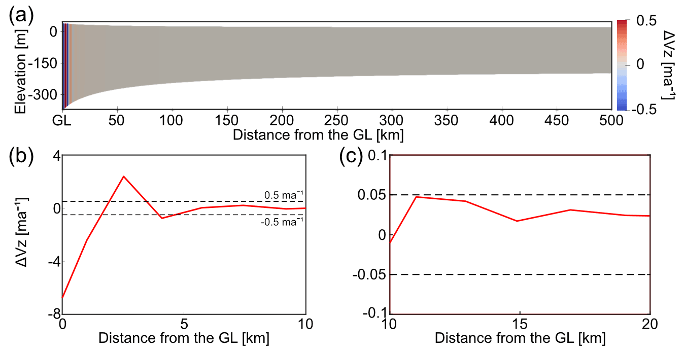
Figure 3 MISMIP EXP 1 synthetic experiment (Sect. 3.1). (a) Differences between the vertical velocity calculated using Eq. (2) and the full Stokes vertical velocity obtained by Elmer/Ice, and (b) transect values (red) from (a) for the first 10 km away from the GL and at 0 m elevation. Dashed black lines represent the ±0.5 m a⁻¹ interval, and (c) transect values (red) from (a) between 10 to 20 km away from the GL and at 0 m elevation. Dashed black lines represent the ±0.05 m a⁻¹ interval.

3.2 Numerical uncertainties in the predicted age–depth fields – NumDiff

Uncertainties due to numerical diffusion in the synthetic test case are highlighted in the horizontal direction using the LMI–CMI delineation line (Fig. 4a) and vertically at a cross-section near x=30 km (Fig. 4b). In both cases, the misfit between numerical and analytical solution decreases with an increase in the number of vertical layers. The mean error in the position of the delineation line decreases from ∼50 m for 10 vertical layers (vertical grid size of around 40 m) to ∼10 m for 200 vertical layers (vertical grid size of around 2 m). Overall, the error is only slightly reduced for more than 100 vertical layers. The kink in the age–depth profile is, to a certain extent, diffused over a depth interval of approximately 25 m with the age of ice being too high in the LMI and too low in the CMI (Fig. 4b). Because of this symmetry, the deflection point of the predicted age–depth profile coincides with the LMI–CMI transition (vertical line in Fig. 4b). The extent of this diffusive zone increases with increasing simulation runtime (t_m). It is therefore necessary to minimize the simulation runtime, and here this is done by choosing t_m=300 a, which corresponds to the advection time from the grounding line to the ice-shelf front. Choosing longer t_m will not add more information. Stream tracing for a fixed velocity field is not affected by the simulation runtime and reliably captures the analytical LMI–CMI transition. This will be used in the following real-world scenarios as an additional control.

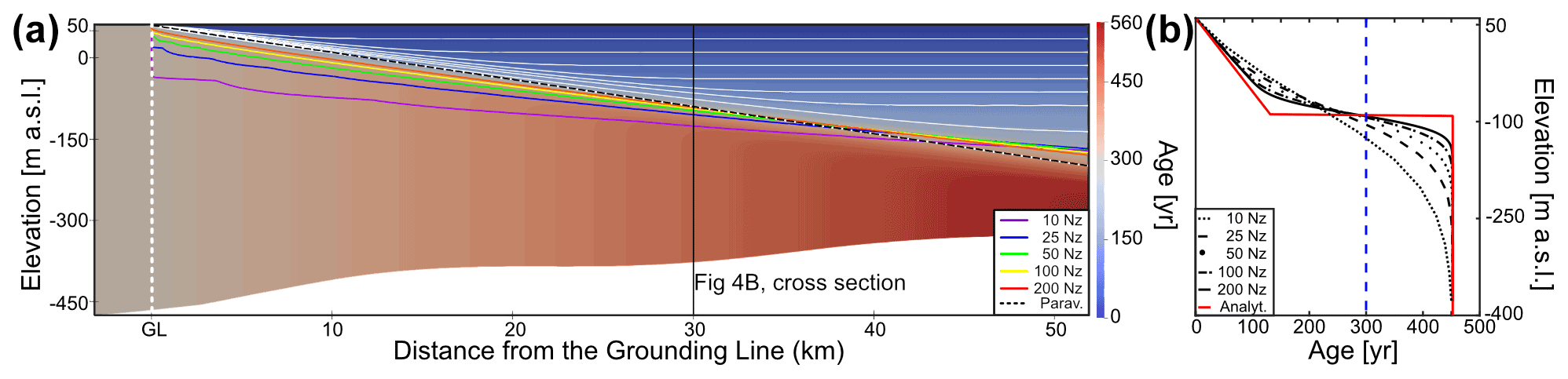
Figure 4 NumDiff experiment (Sect. 3.3). (a) Modeled age field and the delineation line between locally accumulated ice and the advected ice for a different number of vertical layers, N_z (see legend), stream tracer solution from Paraview (black dashes), and analytically calculated delineation (white dots between black dashes). White lines in the LMI represent isochrones. (b) Vertical profile of the ice-shelf age for different N_z at 30 km away from the grounding line. The analytical solution is represented by the red line. The blue line represents the value of the age chosen for the contours in Fig. 4a.

3.3 Predicted 3D stratigraphy of the Roi Baudouin Ice Shelf – RBIS experiment

The predicted age fields along transects D1–D1^′ and D2–D2^′ (located in Fig. 1a) show significant differences in the position of the LMI–CMI boundary, as well as the volume, between these two ice masses in the western (D1–D1^′) and eastern (D2–D2^′) part of the ice shelf (Fig. 5). In the west, the D1–D1^′ transect mainly consists of CMI, and the position of the LMI–CMI boundary is shallow throughout the transect. We find the opposite conditions in the eastern part of the shelf, where the D2–D2^′ transect is dominated by LMI, and the last 20 km leading to the terminus consists solely of LMI. This is also reflected in the deeper position of the LMI–CMI boundary throughout the transect, as well as wider spacing between isochrones in the LMI. The transects D1–D1^′ and D2–D2^′ are along straight lines, not fully following the flowline (Fig. 1a). Older ages of ice occurring in the CMI along that transect originate from the slower flowing margins containing older ice.

Figure 5 RBIS experiment. Modeled age profiles along (a) D1–D1^′ and (b) D2–D2^′ profiles shown in Fig. 1a. Direction of ice flow is from left to right. White lines depict five isochrones at constant intervals from the surface (age = 0) to age = 450 a. The bottom isochrone (black line) in each transect approximates to the LMI–CMI boundary (age = 500 a).

Across-flow cross-sections C1–C1^′, C2–C2^′ and C3–C3^′ show large variations in both the modeled age and position of the LMI–CMI boundary across each section (Fig. 6). The modeled age pattern follows the horizontal velocity field: areas with large horizontal velocities also have a shallow LMI–CMI boundary and correspondingly older ages in the CMI. In contrast, a deeper LMI–CMI boundary and correspondingly older CMI ages occur where the ice flow is slow. Overall, the spatial extent of the LMI / CMI ratio varies greatly across the ice shelf with the largest values in the eastern parts where some extensive parts are entirely sustained by LMI (Fig. 10). The western and the central parts of the ice shelf mainly consist of CMI. The inferred LMI–CMI boundaries, solved using Eq. (1), are broadly consistent with the alternative approach of stream tracing from seed points located at the grounding line (Fig. 6).

Figure 6 RBIS experiment. Modeled age profiles along (a) C1–C1^′, (b) C2–C2^′ and (c) C3–C3^′ transects shown in Fig. 1a. Direction of ice flow is into the image. White lines depict 10 contours at constant intervals from the surface (age = 0) to age = 450 a. The bottom isochrone (black line) in each transect approximates the LMI–CMI boundary (age = 500 a). Black dots correspond to the LMI–CMI boundary calculated using stream tracing.

In order to compare the modeled ice-shelf stratigraphy with observations, we visualize equally spaced isochrones from our predicted age field with the internal reflection horizons (IRHs) in the radar data along the transects A–A^′ (eight IRHs, Fig. 7) and B–B^′ (two IRHs, Fig. 8). Cross-cutting of observed IRHs over modeled isochrones reflects imperfections in the model and in the applied boundary conditions. Because the age of the IRHs is unknown, we choose the predicted isochrones and observed IRH with similar mean depth for a one-to-one comparison (Nereson et al., 1998). Starting from the top, the predicted ages of the radar reflection horizons along transect A–A^′ are 28, 45, 73, 110, 140, 175, 230 and 305 years. Across transect B–B^′, perpendicular to the ice flow, the predicted IRH ages are 20 and 100 years. Earlier kinematic approaches use either the directly modeled depth of isochrones (Arcone et al., 2005) or the age field (Eisen, 2008). We follow the latter approach and obtain isochrones through contouring the finite-element age field. The predicted isochrone that is closest to the observed one in mean depth is used for comparison. Ages are also extracted at the coordinates of the observed isochrones, and the model–data misfit then corresponds to the de-meaned differences acknowledging that the age of the observed isochrone is unknown. Deviations from the mean accordingly highlight systematic misfits along the profile. Following the observed IRHs from the surface towards the bottom for A–A^′ (IRH1-IRH8) and B–B^′ transects (IRH9, IRH10), the standard age deviation for each IRH equals as follows: IRH1: 7; IRH2: 9; IRH3: 14; IRH4: 18; IRH5: 17; IRH6: 19; IRH7: 14; IRH8: 16; IRH9: 9; and IRH10: 17 years.

The misfits, as exemplified by deviations from the mean age, have systematic long (>5 km) and short (<5 km) wavelength components. Close to the grounding line the predicted ages of IRHs (IRH1-IRH8) appear systematically too old, and the trend then reverses farther downstream (Fig. 9). Smaller-scale deviations prominently correlate with, e.g., surface troughs in the topography. Such patterns are most likely indicative of an under-resolution and systematic bias in the surface accumulation rates, but other options are also possible (Sect. 4.2).

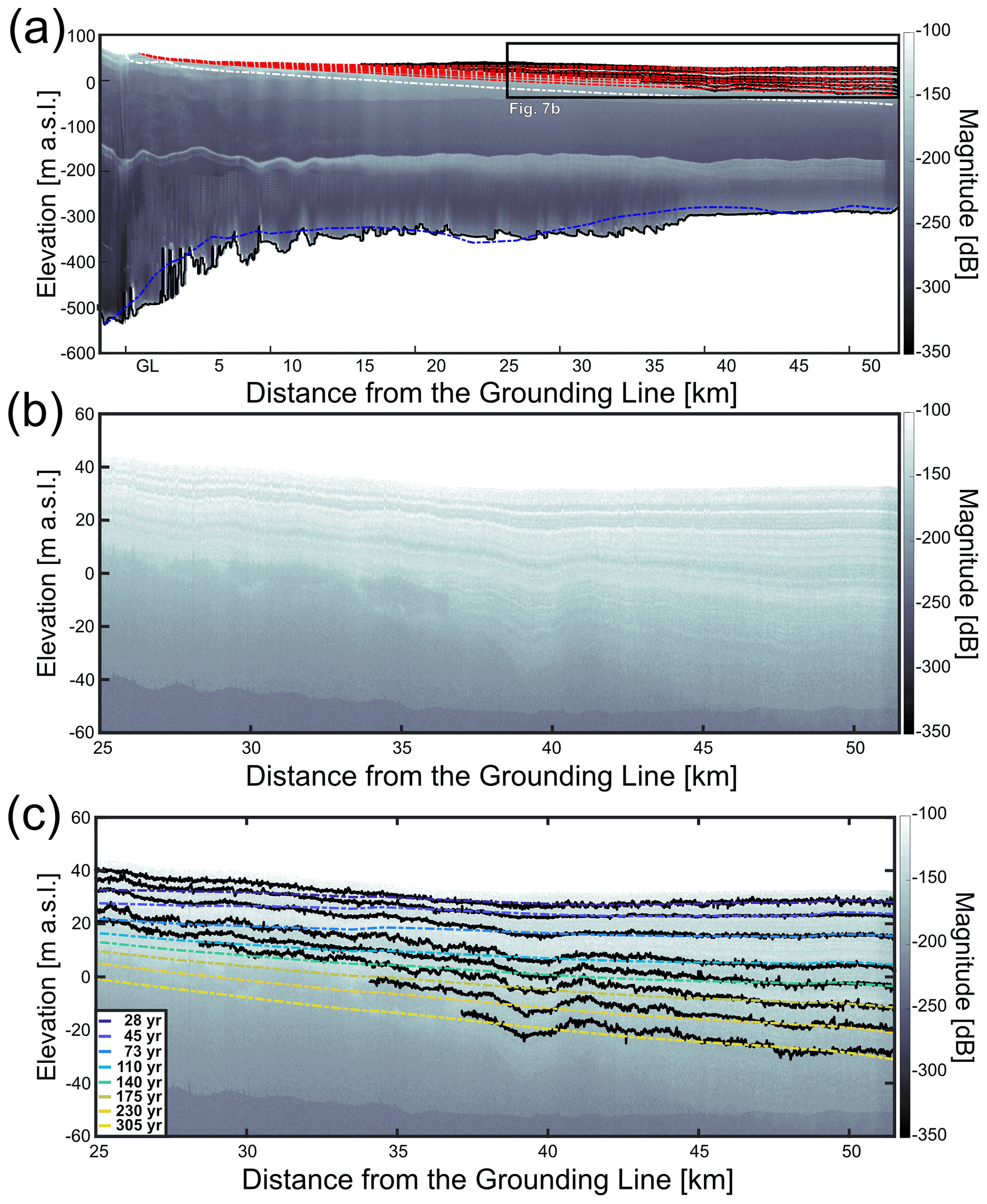
Figure 7 Comparison between radar observations and model output along A–A^′ transect (located in Fig. 1a). Direction of ice flow is from left to right. (a) Radar image of the modeled A–A^′ transect. Black lines represent digitized radar internal reflection horizons IRH1-IRH8, red lines represent modeled isochrones, and the white dash-dotted line represents the LMI–CMI boundary. At the ice shelf–ocean boundary, the blue line is the ice-shelf base used in the model (BedMachine Antarctica), and the black line is the ice-shelf bottom picked from the radar image. Around 200 m of elevation, the prominent white reflection in the radar data is a multiple from the ice surface. (b) Zoomed-in domain shown in the black rectangle in (a). Black lines are picked radar internal reflection horizons. Color dashed-dotted lines (presented in the same order as in the legend) show predicted isochrone geometry and absolute ages (legend).

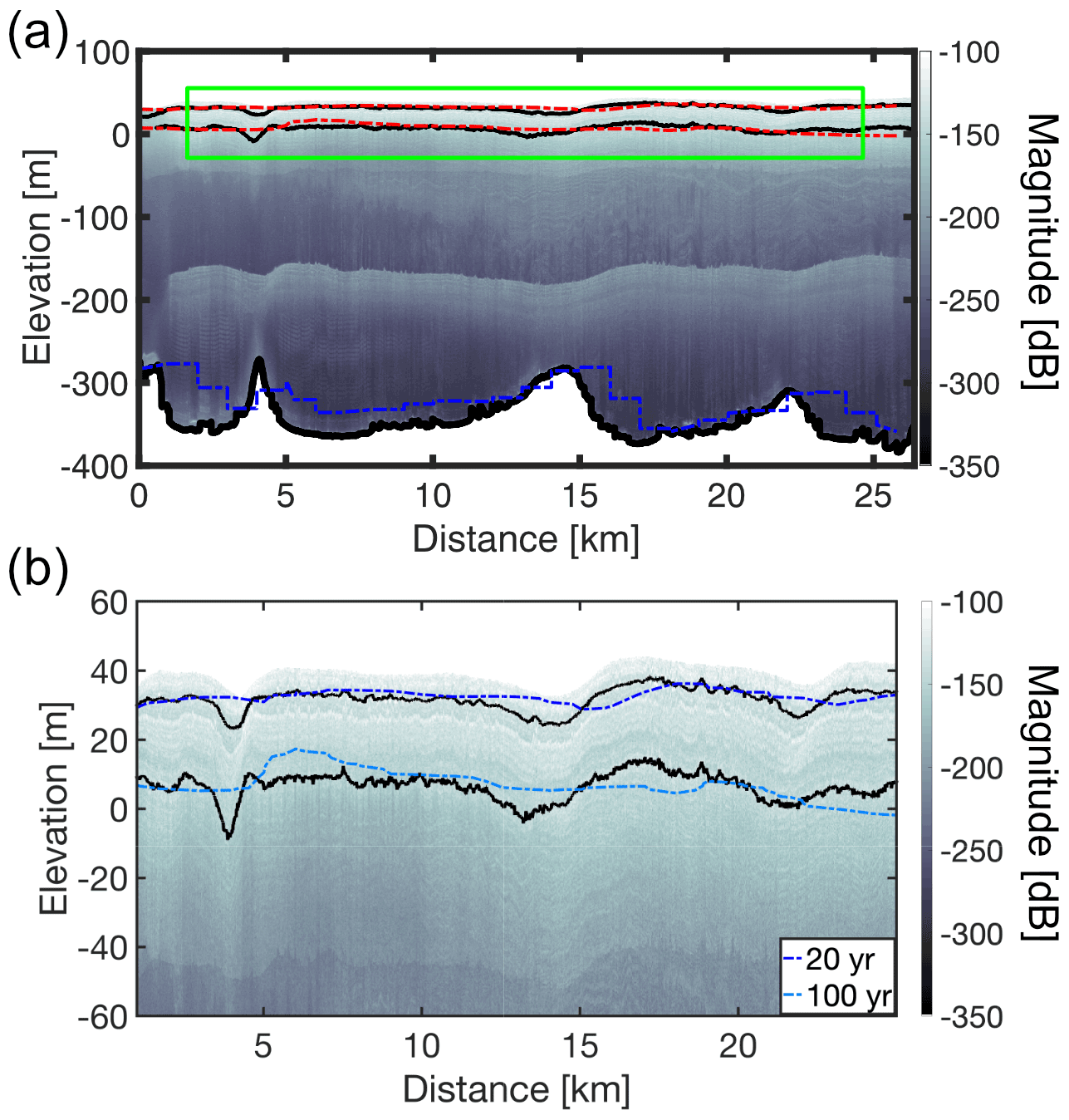
Figure 8 Comparison between radar observations and model output along B–B^′ transect (located in Fig. 1a). (a) Radar image of the modeled B–B^′ transect. Black lines represent picked radar internal reflection horizons IRH9 and IRH10, and red lines represent modeled isochrones. At the ice shelf–ocean boundary, the blue line is the ice-shelf base used in the model (BedMachine Antarctica), and the black line is the ice-shelf bottom picked from the radar image. Around 200 m of depth, the white reflection in the radar data is a multiple reflection from the ice surface. (b) Zoomed-in domain shown in the green rectangle in (a). Black lines are picked radar internal reflection horizons. Color dashed-dotted lines (presented in the same order as in the legend) show predicted isochrone geometry and absolute ages (legend).

4 Discussion

4.1 Limitations of the predictions and comparison to observations

Systematic mismatches between modeled stratigraphy and observations can be attributed to multiple reasons such as (1) numerical diffusion, (2) the applied boundary conditions, (3) violation of the shallow-shelf approximation, (4) violation of the steady-state assumption, and (5) underresolved surface accumulation or basal melt-rate fields. In the following, we discuss these effects separately.

Numerical diffusion (Fig. 4) is inherent when solving the full advection problems, such as the age equation (Eq. 1; Greve et al., 2002). Increasing the vertical resolution is the best way to counterbalance this effect, and here we found that 100 vertical layers (N_z) provide a good compromise between computation runtime and loss of accuracy. Importantly, the imprint of diffusion increases with simulation runtime t_m, which is why t_m should be set to the maximum characteristic time given by the ratio of length and average velocity of the respective ice shelf. The degree of diffusion for any simulation can be quantified by comparing the LMI–CMI boundary with stream tracing which is independent of the simulation runtime. Moreover, the age solver itself can be replaced with other methods to solve the age equation (e.g., Born, 2017; Born and Robinson, 2021), as the underlying host model for the velocities is simplistic and can be easily implemented in other frameworks.

The choice of a constant age value, $A(z,x=\text{GL})=t_m$, at the inflow boundary currently precludes analysis of the radio stratigraphy in the CMI zone. In many examples, such as in our test case at RBIS or also in large parts of the McMurdo Ice Shelf (Das et al., 2020), this is acceptable, as the stratigraphy of inflowing tributary ice streams into the ice shelves is often not well preserved. Nonetheless, in areas where slow-flowing ice enters the ice shelf, the stratigraphy in the CMI may well be intact so that the boundary condition applied is unsatisfactory. In principle, this can be solved by making the inflow boundary condition one of the free parameters in the corresponding inverse problem or by using the output of a large-scale model as input for the inflow boundary of a nested ice-shelf simulation.

The differences between the full Stokes Elmer/Ice vertical velocity and the analytical formula (Eq. 2) are small over the majority of the ice shelf, except within 5 km distance from the grounding line (Fig. 3), where more stress gradients are relevant than considered in SSA. More specifically, this includes an oscillating pattern that emerges at the transition between the grounded ice sheet and the floating ice shelf (Lestringant, 1994; Durand et al., 2009). Ice-shelf channel closure from lateral inflow is one example that is not adequately captured by the SSA (Drews, 2015; Wearing et al., 2021). Moreover, the surface accumulation rates likely change over these small spatial scales as discussed below. Also not included in this comparison are velocity modulations through ocean tides (e.g., Marsh et al., 2013; Rosier et al., 2017; Drews et al., 2021), although over the long timescales considered here this effect is likely to be negligible.

As the model domain starts at the grounding line, the incomplete kinematic model will predict an incorrect age profile for the shallow LMI at this location. This error will be maintained in the stratigraphy downstream. However, this effect is small because (1) the missed positive and negative oscillations will, to a certain extent, average out and (2) the ice residence time (typically several tens of years) across the grounding zone is an order of magnitude smaller than the characteristic time of ice shelves (typically many hundreds of years).

The steady-state assumption in Eq. (2) can, in principle, be extended to also include transient thickness changes as observed by satellite altimetry (Paolo et al., 2015), but the kinematic model does not handle the implied change in ice geometry. Therefore, an extension to transient cases requires more work – especially on constraining transient changes in ice geometry and velocities, as well as in atmospheric and oceanic forcings. However, a systematic mismatch between the predicted and observed stratigraphy can be treated as a first-order metric that transient changes have occurred in the first place.

Given that the vertical velocities in Eq. (2) are approximately 9 times more sensitive to surface accumulation rate ($\dot{a}$) than to basal melt rate ($\dot{b}$) (Drews et al., 2020), it is imperative to have a well-constrained surface accumulation field for reliable predictions of the isochronal stratigraphy. Future temporal changes or general uncertainties in the surface accumulation and basal melt-rate fields will propagate linearly into changes in the position of the LMI–CMI boundary (Eqs. 1 and 2). If surface accumulation is well constrained and if the ice shelf is in steady state, the forward model presented here is a step towards an inverse approach to reconstruct basal melt rate which is arguably the least well known.

It is a logical next step to extend this method to other Antarctic ice shelves. The analysis of spatial variations in the LMI–CMI boundary across the ice shelves links to studies investigating ice-shelf rheology and its spatial variations from inverse modeling (Larour et al., 2005; Khazendar et al., 2011). They find zones of stiffer ice and softer ice caused by the variability in ice temperature. In particular, ice from tributary ice streams is colder and stiffer. In our case, this will be mapped as CMI. Therefore, the spatial variations in the LMI–CMI boundary will likely reflect spatial variations in viscosity, implying that ice shelves with large LMI–CMI contrast also have a large contrast in viscosity.

Mapping and analyzing spatial variations in the LMI–CMI boundary can serve as a proxy for the sensitivity of the respective ice shelves to atmospheric or oceanographic perturbations (Levermann et al., 2020; Gilbert and Kittel, 2021). The buttressing capacity of ice shelves depends on their geometry (thickness) and structural integrity. The geometry of ice shelves dominated by LMI is hence controlled by the atmosphere, and consequently they are more susceptible to the projected changes in surface accumulation rates than ice shelves which are dominated by CMI. An atmospheric modeling study by Gilbert and Kittel (2021) suggests that the projected future increase in surface temperature nonlinearly increases the amount, duration and extent of surface melt and runoff, which increases vulnerability to hydrofracturing of ice shelves dominated by LMI. On the other hand, ice shelves dominated by the CMI will be more susceptible to the projected increase in basal melt (Naughten et al., 2018; Levermann et al., 2020; Gilbert and Kittel, 2021).

Furthermore, the predicted isochronal field can be tested against radar observations, particularly farther seawards, where the typically well-ordered stratigraphy of the LMI occupies a larger fraction. Systematic mismatches between observations and predictions can then be discussed in terms of the forcing fields ($\dot{a}$, $\dot{b}$, V_H) and transient changes thereof. We further discuss such a comparison for the Roi Baudouin Ice Shelf.

4.2 Model–data comparison at the Roi Baudouin Ice Shelf, East Antarctica

The across- and along-flow cross-sections shown in Figs. 5 and 6 present modeled results of the radar stratigraphy in the Roi Baudouin Ice Shelf for a given set of surface accumulation rate ($\dot{a}$) and basalt melt-rate ($\dot{b}$) fields. These fields can give guidelines for the expected age–depth relationships when interpreting the stratigraphy from ice cores obtained from ice shelves (e.g., Hubbard et al., 2013). They can also be used as a planning tool for radar surveys targeting the LMI where the stratigraphy is typically more intact than in the CMI.

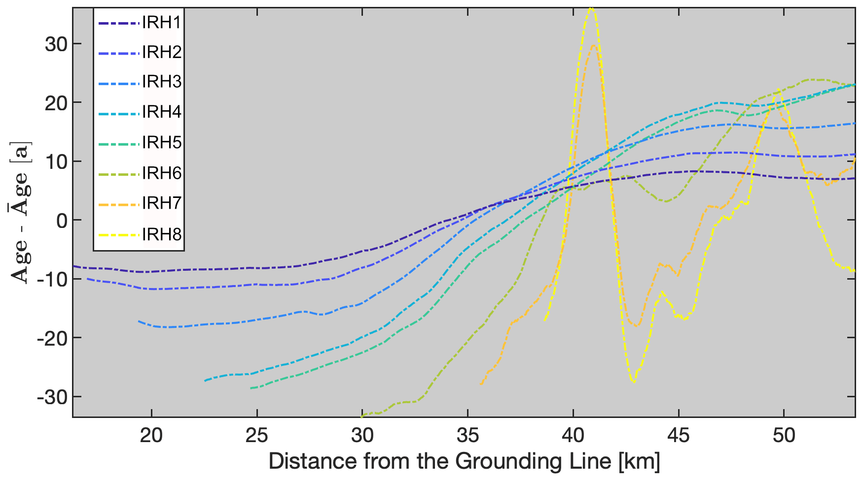
Figure 9 Modeled age deviations from picked internal reflection horizons along profiles from Fig. 7, represented by lines IRH1–IRH8 starting from the surface towards the bottom.

The comparison of modeled isochrones with observations along A–A^′ captures the expected trend of a progressively increasing volume of the LMI, where the LMI–CMI boundary reaches a depth of approximately 40 m over a 50 km along-flow distance (Fig. 7a). In the radar profile, IRHs only develop approximately 15 km downstream of the grounding line, although surface accumulation rates are positive throughout. Consequently, the model predicts the formation of LMI everywhere. In this specific example, this can be explained with surface meltwater infiltration in austral summers, as well as with the existence of supraglacial lakes in the area upstream of the ice shelf (Stokes et al., 2019). Meltwater forms at the surface due to ice–albedo feedbacks in a narrow belt near the grounding line (Lenaerts et al., 2017). This infiltration prevents the formation of a coherent radar stratigraphy even if the yearly averaged surface accumulation is positive.

Both the depth of the modeled isochrones (Figs. 7c and 8) and the age variations along the IRHs (Fig. 9) show that the modeling result better reproduces IRHs closer to the surface. Further away from the grounding line, the model results overestimate the depth of the IRHs and do not reproduce the large-scale trend until around the last 5 km for deeper to 15 km for shallower IRHs. Standard deviations between observations and predictions span between 7 and 19 years. Reasons for this are numerous and cannot be fully resolved here. It is possible that either the surface accumulation rates near the grounding line are too high or that the basal melt rates are too low. For both cases (or a combination thereof), the misfits of predicted isochrones and IRHs add cumulatively over time and hence systematically increase with depth. Transient signatures in the applied fields are also a possibility and would need to be tested using inverse modeling. The same ambiguities also exist in principle for the smaller-scale variability around ice-shelf channels (Fig. 8). However, here it is most likely that this is rather caused by an under-resolving of spatial processes in atmospheric precipitation which are known to sensitively depend on small-scale changes in surface slopes but are not yet resolved in the reanalysis data (Drews et al., 2020; Van Liefferinge et al., 2021).

Moving further away from the grounding line, we find the comparison of model predictions and observations on larger spatial scales encouraging, providing support that this particular catchment has not undergone large-scale changes in recent time. This is in line with other studies in this area that inferred similar statements in terms of ice-dynamic stability and linked atmospheric precipitation patterns on ice rises (Drews, 2015; Callens et al., 2016). Nonetheless, whether the presented misfit is dominated by local underestimation or potential small transient changes in model forcings (surface accumulation rate, basal melt rate) is currently unclear and should be investigated in future studies.

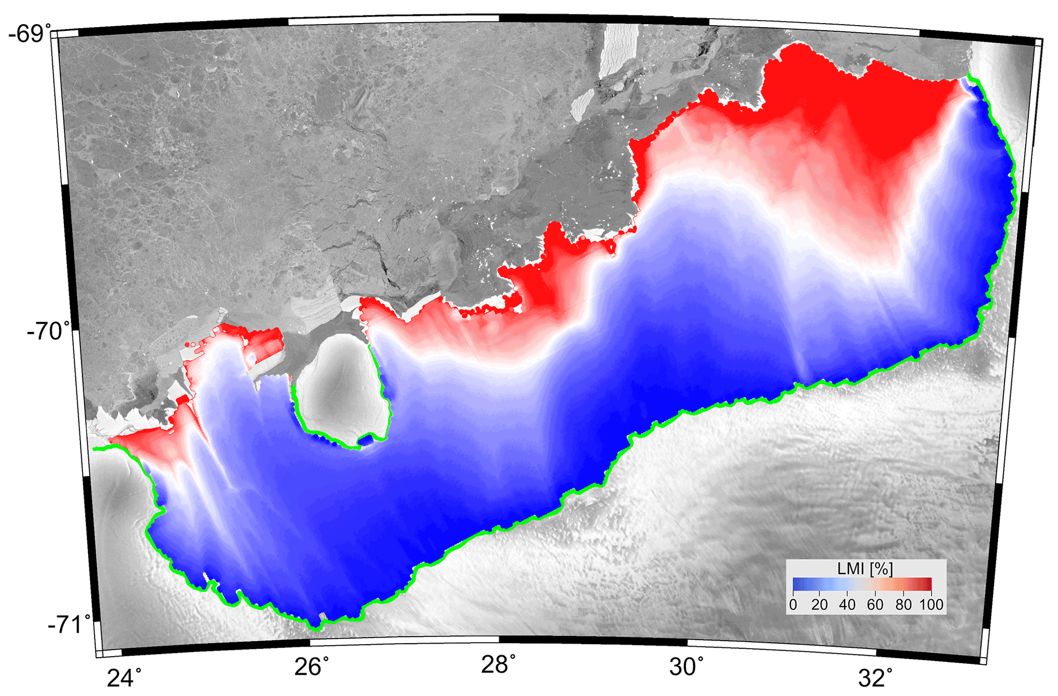
Figure 10 Percentage of local meteoric ice (LMI) over the ice shelf inferred from the steady-state age–depth fields. The white contour marks the LMI–CMI ratio of 0.5. Areas marked in red are dominated by CMI and areas in blue by LMI. The green curve represents the position of the grounding line used in the model.

4.3 Spatial variations in the percentage of locally accumulated ice

Mapped spatial variations show a non-uniform distribution in the percentage of LMI across the ice shelf (Figs. 5, 6 and 10). The differences between the western and eastern parts are reflected in the surface velocity contrast between them (Fig. 1b). Unlike the western part, where the composition of the shelf is clearly dominated by CMI advected from the West Ragnhild Glacier, in the eastern part the total ice volume is dominated by LMI, but the LMI–CMI ratio cannot be directly understood from the input data (Fig. 1).

This potentially makes the eastern part more likely to move out of close to steady-state conditions in the future, as its composition mainly depends on local surface accumulation – which is prognosed to decrease (Kittel et al., 2021). Central and western areas of the shelf are less susceptible to these localized changes in mass input and output, as they mainly consist of ice accumulated on and advected from the grounded ice sheet, where future projections for the end of this century project an increase in overall surface accumulation for the +1.5 and +2.5 ^∘C scenarios (Kittel et al., 2021).

4.4 Future development

In future applications, the analysis of the spatial variability in the LMI–CMI pattern can be expanded to give insights into its susceptibility to future changes in the atmospheric and oceanographic conditions for all ice shelves around Antarctica. Secondly, mismatch between model output and observations can be used to refine atmospheric precipitation and ocean-induced melting on the finer spatial scale provided by the radar observations. Coupling with a larger-scale ice-sheet model can improve the inflow boundary condition so that also the CMI can be included in this approach.

5 Conclusions

The method here predicts the steady-state ice stratigraphy of an ice shelf using observations (ice geometry, surface velocities, surface accumulation rate, basal melt rate) and a simple kinematic ice-flow model. In synthetic examples, we show that the predicted vertical velocities correspond well to a full Stokes solution except in the first 5 km near the grounding line. Because the kinematic model is numerically efficient, it is possible to counterbalance numerical diffusion when solving the age equation with a high vertical resolution of 100 layers or more. Applications of this approach include calculation of the ratio between local meteoric ice (LMI) and continental meteoric ice (CMI) of ice shelves which serves as a first-order metric of the susceptibility of individual ice shelves to changes in atmospheric and oceanographic forcings. Moreover, comparing predictions with observations from radar data provides a tool to estimate whether or not, for the atmospheric and oceanographic forcing from today, the stratigraphy which typically develops over many hundreds of years is in steady state.

The methodology is illustrated using the Roi Baudouin Ice Shelf in East Antarctica as a test case. The model–observation mismatch decreases moving away from the grounding line, which could be due to unresolved variability in surface accumulation rates and basal melt rates in the input data for that area. The LMI / CMI ratio of this particular ice shelf varies strongly in the east–west direction and serves as a good example for two types of endmember ice shelves that are either primarily sustained by the local surface accumulation or by the ice flux of a tributary glacier. These will respond differently should atmospheric and oceanic circulation patterns change in the near future.