the Creative Commons Attribution 4.0 License.
the Creative Commons Attribution 4.0 License.
 | 25 Oct 2022
The effect of hydrology and crevasse wall contact on calving
Christian Schoof
Anthony Peirce
Calving is one of the main controls on the dynamics of marine ice sheets. We solve a quasi-static linear elastic fracture dynamics problem, forced by a viscous pre-stress describing the stress state in the ice prior to the introduction of a crack, to determine conditions under which an ice shelf can calve for a variety of different surface hydrologies. Extending previous work, we develop a boundary-element-based method for solving the problem, which enables us to ensure that the faces of crevasses are not spuriously allowed to penetrate into each other in the model. We find that a fixed water table below the ice surface can lead to two distinct styles of calving, one of which involves the abrupt unstable growth of a crack across a finite thickness of unbroken ice that is potentially history-dependent, while the other involves the continuous growth of the crack until the full ice thickness has been penetrated, which occurs at a critical combination of extensional stress, water level and ice thickness. We give a relatively simple analytical calving law for the latter case. For a fixed water volume injected into a surface crack, we find that complete crack propagation almost invariably happens at realistic extensional stresses if the initial crack length exceeds a shallow threshold, but we also argue that this process is more likely to correspond to the formation of a localized, moulin-like slot that permits drainage, rather than a calving event. We also revisit the formation of basal cracks and find that, in the model, they invariably propagate across the full ice shelf at stresses that are readily generated near an ice shelf front. This indicates that a more sophisticated coupling of the present model (which has been used in a very similar form by several previous authors) needs modification to incorporate the effect of torques generated by buoyantly modulated shelf flexure in the far field.
- Article
(3303 KB) - Full-text XML
- BibTeX
- EndNote


Calving is the formation of fractures that separate newly formed icebergs or smaller pieces of ice from a contiguous ice shelf or marine-terminating glacier. In marine ice sheet and outlet glacier models, the choice of a “calving law” has a significant effect on steady-state configurations (Schoof et al., 2017; Haseloff and Sergienko, 2018). Despite its importance, there is currently no comprehensive theory for calving.
A variety of different approaches have been used to model fracture in ice. Aside from early heuristic “zero-stress”-type models (Nye, 1957; Nick et al., 2010; Todd and Christoffersen, 2014), these are primarily discrete element models (which do not pretend to represent ice as a continuum); linear elastic fracture mechanics models, which focus on one or a few discrete cracks; and continuum damage mechanics models, which treat calving as the result of the density of microfractures accumulating to generate a macroscopic crevasse that penetrates through the ice thickness (Larour and Aubry, 2004; Benn et al., 2007; Cook et al., 2014; Levermann et al., 2012; Borstad et al., 2012, 2013; Krug et al., 2014; Bassis and Jacobs, 2013; Mobasher et al., 2016; Yu et al., 2017; Benn et al., 2017; Todd et al., 2018). In addition to different assumptions about the basic physics involved, there are additionally different numerical approaches that can be applied to the resulting models, especially in the case of linear elastic fracture mechanics (Touvet et al., 2011; Tsai and Rice, 2012; Jiméneza et al., 2017; Lipovsky, 2020).
One of the most significant challenges is to capture fracture evolution in an ice sheet or ice shelf that flows viscously over long timescales (Yu et al., 2017), owing to the very different timescales and physical processes involved. Damage mechanics attempts to bridge that gap with a smoothly evolving damage function describing fracture density. By contrast, direct application of linear elastic fracture mechanics only attempts to capture short-term changes in stress during the formation of a fracture and their role in fracture propagation. In this paper, we take the latter approach, studying how elastic fracture propagation over short timescales is controlled by a viscous pre-stress, overburden and water pressure in a crevasse.
Our model is a generalization of the crack penetration models for ice shelves in van der Veen (1998a, b) and Lai et al. (2020). Like these authors, we focus on vertical fracture propagation in two dimensions under plane strain conditions, omitting complications introduced by three-dimensional rift formation (Lipovsky, 2020), and consider cracks that are far from either the ice front or the grounding line. We formulate the model (and the corresponding numerical solution method) for arbitrary two-dimensional geometries and impose contact constraints that prevent opposite sides of a crack from interpenetrating. In particular, we extend the completely fluid-filled and completely dry-crack scenarios in Lai et al. (2020) to more general hydrologies, focusing on surface cracks in which the water level is either prescribed or constrained by a finite volume injected into the crack. In addition, we revisit the case of water-filled basal cracks previously studied in van der Veen (1998b) and Lai et al. (2020).
In order to deal with crack face contacts and, ultimately, with general ice geometries, we have to abandon the use of tabulated Green's functions previously pioneered in van der Veen (1998a, b) and Lai et al. (2020). In this paper, we employ a boundary element method to compute stress fields in the ice. We show how possible steady-state crack configurations change when stress, thickness and hydrological forcing parameters are varied and use these results to derive calving laws for two-dimensional ice shelves. Depending on parameter combinations, we find that calving can occur either by steady-state crack lengths continuously growing to span the entire ice thickness or by a steady-state crack that partially penetrates the ice being destabilized and growing across the full thickness of the ice.
The paper is organized as follows: we formulate the fracture model of van der Veen (1998a, b) and Lai et al. (2020) in terms of partial differential equations in Sect. 2.1, separating the elastic stress field induced by the introduction of a fracture from a viscous pre-stress and accounting for contact constraints that prevent crack faces from interpenetration. We also formulate the crack propagation criterion we use in Sect. 2.2. Following Lai et al. (2020), we reduce the parameter space of the model through non-dimensionalization in Sect. 2.3 and sketch the numerical method used in Sect. 3, with further detail relegated to Appendix B. Results are presented in Sect. 4, where we focus on the case of a single crack incised into a parallel-sided slab of ice; in that case, the viscous pre-stress is known exactly, and more general ice geometries will be considered in a separate paper. As in van der Veen (1998a, b) and Lai et al. (2020), we begin by studying the dependence of the stress intensity factor on crack length in Sect. 4.1, identifying the range of steady states accessible for individual parameter combinations. We consider the effect of incorporating the contact constraints into the model in Sect. 4.2–4.3. Section 4.4 systematically explores the dependence of steady-state configurations on parameter variations, allowing us to describe how changes in forcing can precipitate calving in Sect. 4.5. In Sect. 5, we use these results to formulate calving laws that can be used in large-scale models, focusing on the distinction between calving laws that require a knowledge of the history of the ice shelf from those that can be formulated purely in terms of current forcing parameters in the form of extensional stress, ice thickness and hydrology. We summarize our findings and point to some of their limitations in Sect. 6, where we identify torque-driven calving as being poorly represented in the model as formulated, which does not incorporate the effect of changes in buoyancy due to vertical deflections.

Figure 1Cross-section geometry of a marine ice sheet and the geometry of the problem: part of a floating ice shelf with a surface or bottom crevasse.
2.1 Model description
We employ a Cartesian coordinate system , with a horizontal x axis and z measured relative to sea level. We denote the domain by Ω and its boundary by ∂Ω, with an outward-pointing unit normal n. Let σij be the Cauchy stress tensor. In common with many other fracture problems (Zehnder, 2012; Crouch and Starfield, 1983), we consider only the quasi-static case here, so
where is acceleration due to gravity and the summation convention is used; Eq. (1) is equally applicable to the equivalent, purely viscous flow problem that applies at longer timescales.
In order to cast the problem previously solved by van der Veen (1998a, b) and Lai et al. (2020) in the form of partial differential equations (appropriately generalized to take greater account of variations in surface hydrology and allowing for contact between crack faces as described below), it is necessary to assume a compressible Maxwell-type viscoelastic rheology and separate the stress tensor σij into a viscous pre-stress that existed just prior to crack propagation and an elastic stress generated by crack propagation on timescales much faster than a single Maxwell time (Christensen, 1982),
A derivation of this decomposition (see also Lipovsky, 2020, for a similar decomposition into a pre-stress) from first principles is included for completeness in Appendix A. We assume that the viscous pre-stress is known from solving a Stokes flow problem for the domain just prior to introduction of the crack and therefore satisfies the boundary conditions (5–7) stated below for the exterior boundaries of the domain.
Our focus will be on finding the elastic stress field that results from the introduction of cracks. Our model only accounts for an in-plane displacement field (relative to particle positions immediately before the introduction of the crack), with an associated strain:
The decomposition in Eq. (2) is such that is related to the short-term elastic strain εij by an isotropic, linear elastic rheology. This prescribes the elastic stress in terms of strain εij in plane strain conditions as
with the sum over repeated indices running over {1,2}. Here, ν is Poisson's ratio and is the plane strain modulus, with E being Young's modulus and both ν and E′ assumed to be constant.
The upper surface at z=s (Fig. 1) is traction-free; therefore
where σij is the total Cauchy stress as before. At the lateral boundaries at , we impose a normal stress, the sum of a cryostatic contribution, and an imposed extensional (or “resistive”) stress Rxx (equal to if μ is viscosity and U is far-field ice velocity; see also van der Veen, 1998a, b):
At the base of the ice z=b, we have hydrostatic pressure from the ocean:
Note that, in this paper, we will solve the model only for the case of single cracks incised into a wide slab of ice whose upper and lower surfaces before crack formation are parallel, as is also the case in van der Veen (1998a, b) and Lai et al. (2020); the numerical method described is however equally suited to more general geometries and to multiple cracks, both of which we will consider in separate papers. For the parallel-sided slab, the lateral stress field in Eq. (6) naturally results from the viscous deformation of a wide slab of ice in which ice flows as a plug with no vertical shear, for which the viscous stress tensor is simply
Importantly, the stress field defined by Eq. (8), which on its own satisfies lateral stress conditions (Eq. 6), cannot be generated by a compressible elastic rheology (in the sense that there is no displacement field that generates through Eqs. 3–4 above, unless we assume that , corresponding to elastically incompressible ice). This explains our insistence on separation of σij into viscous and elastic parts and , respectively.
For the domain used in Sect. 4 in this paper, Eq. (8) is therefore the appropriate form of the viscous pre-stress; for a more general initial geometry, it is necessary to solve Eqs. (1)–(7) numerically on the uncracked domain first, subject to a purely viscous rheology (that is, putting ) in order to find the viscous pre-stress before introducing the cracks. We will deal with that more complicated procedure in a separate paper (see also Yu et al., 2017).
Cracks are internal boundaries on which displacement may be discontinuous and stress boundary conditions can be prescribed. We define an outward-pointing unit normal n± to each side of the crack, denoting the left by the superscript + and the right by −. By outward-pointing, we mean that, on each side, n± points towards the crack rather than the interior of the domain. In the small-strain limit of linear elasticity, the two sides of the crack are parallel and . Similarly denoting v± as the relevant limit of an arbitrary vector field v, we can define a jump in its normal component across the crack as or, equally, in subscript notation . In that notation, crack width w is
Boundary conditions on either the top or the bottom crack can be expressed as
where pf is fluid pressure in the crack. These conditions ensure that normal stress is continuous and exceeds fluid pressure where the crack is closed or equals fluid pressure where the crack is open. In addition, we assume that shear stress vanishes even when the crack walls re-contact each other, thus assuming them to be smooth and not subject to healing on the timescale under consideration:
The stress conditions above hold for both faces of the crack, in the sense of σij being evaluated as the limit taken from either side of the crack, with n being the outward-pointing unit normal that corresponds to the side from which the limit is taken. Here pf is the fluid pressure inside any of the cracks, given by
in a surface crack, and
in a bottom crack. hw is the depth of the water level in the surface crevasses below the upper surface z=s in the surface crevasses.
We consider two basic scenarios as possible end-members of surface hydrological systems. The first is a prescribed water level hw below the ice surface as previously used by van der Veen (1998a). This is the “wet” end-member of surface hydrological systems, where a large and well-connected reservoir of water (presumably a subsurface aquifer) is able to rapidly supply water to the crack and maintain the water level during crack propagation. The second scenario involves a prescribed water volume in the surface crack, representing a water-limited system with an isolated surface crack that is not rapidly resupplied with water as it lengthens; in this case, the water level hw will generally drop as the crack propagates. The latter hydrology is also motivated by Nick et al. (2010), who use the somewhat more difficult-to-justify assumption of a prescribed water column height above the bottom the crack (see also Schoof et al., 2017): one would not generally expect the column height to be prescribed in nature, while the similar but not identical assumption of a fixed water volume simply reflects conservation of mass in an isolated surface crack. Further refinement to the two end-member scenarios is likely to be a target for future work: as we will see below, we obtain very different dynamical behaviour depending on whether the water level or water volume is prescribed. Naturally, this also raises the question of how one would observationally constrain hydrology around surface crevasses. In the spirit of a forward modelling study, we focus here on the basic dynamics of the system under the stated assumptions and leave open the question of observational validation.
Let Vw be the prescribed water volume and dt the vertical extent of the crack (see Fig. 1). If all the prescribed water volume can be accommodated in the crack, then there exists an hw> 0 such that
Otherwise, if the prescribed volume cannot be accommodated in the crack, then hw=0 and the excess is stored at the surface. In putting hw=0 when the prescribed volume cannot be accommodated in the crack, we assume that Vw remains comparable to the volume that can be stored in a crack and therefore corresponds to an insignificant water depth at the ice surface when ponded in this way. “Insignificant” here implies that ponded water depth is small compared with the length of the crack: deep surface lakes storing much larger water volumes are beyond the scope of our work.
Note an important caveat to the boundary conditions (12–13): both assume that negligible hydraulic potential gradients are required to drive fluid flow along the cracks as their tips move and the cracks open or close so that water pressure can be treated as hydrostatic in each crack. The propagation criteria in the next section are built around this assumption, which gives a particularly simple way of handling the stability of cracks but likely needs to be superseded by a more sophisticated treatment of water movement in the cracks in future work (Spence and Sharpe, 1985).
We will refer to the constraint requiring a non-negative crack width, w≥0, as the “contact constraint” in the remainder of this paper. Note that van der Veen (1998a, b) and Lai et al. (2020) do not enforce the contact constraint. To reproduce their results, we also consider an alternative (and not always physically viable) set of boundary conditions on the crack, putting
instead of the original boundary conditions (10); the prescription of a fixed water volume or water level remains as described above in that case, except that in the case of a fixed water volume, the integral in Eq. (14) is taken over rather than w so that crevasse wall overlap does not contribute negatively to water volume.
Before we move onto crack propagation in the next subsection, note also the following: in common with van der Veen (1998a, b) and Lai et al. (2020), our formulation does not consider the effect of elastic displacements on the position of the upper or lower boundaries and therefore on changes in water pressure and hence in buoyant support. Our elastic model is based on small strains, which implies that ; with ice thicknesses around H≈1000 m, g≈ 10 m s−2, ρi≈900 kg m−3 and a Young's modulus of E≈109 Pa (Vaughan, 1995), we find strains around 10−2. Over the length scale given by a single ice thickness (relevant to elastic deformation around a crack that penetrates partially through the ice), this implies that elastic displacements are small and buoyant effects are higher-order corrections: a consideration of buoyant effects requires flexure over a longer horizontal length scale (Wagner et al., 2016; Buck and Lai, 2021); formally, deformation at that scale should couple to the model described here via far-field boundary conditions at the lateral sides of the domain through the procedure of asymptotic matching. As in prior work by van der Veen (1998a, b) and Lai et al. (2020), we do not consider that complication here, opting for the simple boundary condition (6) instead. We return to the limitations this imposes in Sect. 6.
With the simpler boundary condition (6) lacking any far-field torque or net shear force, note also that the model above is subject to the following Archimedean flotation solvability condition, which can be derived by integrating Eq. (1) over the domain and using the divergence theorem:
for a parallel-sided slab geometry of thickness with constant s and b, this gives the simple and familiar , .
2.2 Propagation criterion
We follow linear elastic fracture mechanics (Zehnder, 2012) in assuming that fracture propagation can be described by a simple fracture toughness. Near the tip of the crack, the stress field generally becomes singular (except when the crack faces touch with w=0). The stress intensity factor for a mode-I crack is computed as
in a local (r,θ) polar coordinate system centred on the crack tip, with θ=π being tangential to the crack. Crack propagation is assumed to be controlled by a constant fracture toughness KIc, with measured values of KIc for polycrystalline ice lying between 0.1 and 0.4 MPa m (Rist et al., 1996). The crack will not propagate if KI<KIc, while the crack propagates once static KI exceeds KIc.
In a strict sense, the static force balance model can therefore only compute static crack lengths which are such that they ensure that KI≤KIc (meaning the crack may be on the point of moving but remains static), and the length of the crack then becomes part of the solution, rather than being prescribed. A static model is insufficient to understand how cracks grow as the forcing on the system changes, in the form of changes to the excess tension Rxx or the water volume Vw (or, equivalently, to water level depth below the surface hw). If there is only a single crack, its dynamics under changes in parameters are likely to be simple: any such change that reduces the static KI below KIc would leave the crack length unchanged, while increases in static KI above KIc would cause lengthening of the crack until its tip once more attains the static value of KIc (or the fracture propagates all the way through the ice). This heuristic argument results in a simple stability criterion for steady-state cracks, used in Lai et al. (2020): if a slight lengthening of a steady-state crack results in a decrease in KI in the static stress model, then that crack is stable, while it is unstable or marginally stable otherwise.
In the case of multiple cracks, however, not all cracks need to propagate simultaneously or at the same speed, and it is then unclear which cracks should be lengthened until they reach KIc and which cracks will have stress intensity factors below KIc when a new equilibrium is reached. While we ultimately solve the problem only for a single crack in the present paper, the numerical method we use can deal with multiple competing cracks. For the sake of completeness, we therefore describe the method we use to capture dynamic crack propagation below, even though results for competing cracks will be presented in separate papers.
Dynamic propagation of cracks typically reduces the stress intensity factor, and the rate of crack propagation is that which lowers the dynamic KI to the critical value KIc. There are two processes by which this reduction in the stress intensity factor can occur: for sufficiently rapid crack propagation, inertial effects can be the dominant effect (Freund, 1990), or changes in fluid pressure in the crack driven by fluid flow as the crack tip advances and the crack widens can dominate (Spence and Sharpe, 1985). Here we investigate only the former, which is strictly applicable to dry cracks but furnishes a very simple propagation rule. The reason for persisting with this process is that it makes the calving problem tractable in which crack propagation has to be computed for a large set of combinations of forcing parameters.
In general, the computation of KI during fracture propagation then requires a dynamic model in which inertial terms are not omitted in Eq. (1). Solving a time-dependent problem that captures elastic waves renders our just-stated objective of computing fracture propagation for many forcing parameters intractable as it increases the number of dynamical degrees of freedom from the number of cracks to a dynamic displacement field throughout the domain. Short of solving a full dynamic crack propagation problem, we can use the semi-analytical theory of Freund (1990), who considers the situation in which the statically computed KI only slightly exceeds KIc. In that case, inertial terms are only significant in a small boundary layer around the crack tip, and the stress field far from the crack tip can be determined using the static model described above. The stress intensity factor KI at the moving crack tip can then be related to the stress intensity factor computed from the static model KI,stat through
where d is crack length, the dot on d signifies an ordinary derivative with respect to time and K is the “universal function” as computed by Freund (1990); the key property here is that K increases with . Assuming that is small but positive so that the crack will propagate, we can linearize Eq. (18) as , where we have used the fact that the crack is propagating, so KI=KIc. This leads to the simplified propagation equation.
where . Despite the fact that the derivation of this evolution equation for crack length strictly speaking only applies to the case of the static stress intensity factor KI,stat that exceeds the fracture toughness KIc by a small amount, we assume that Eq. (19) holds whenever to facilitate rapid solution. When , the simplest assumption to make is that the crack tip does not evolve, so there is no healing of the crack, in which case we can generalize Eq. (19) as
Note that if, as is implicitly assumed here, crack propagation occurs in a predefined direction (by symmetry vertically, in the examples in this paper), then Eq. (20) represents a dynamical system with as many dimensions as there are cracks: for a given set of crack lengths d and therefore a given domain, the elastostatic problem of the previous section allows the stress field and therefore the KI at each crack tip to be computed uniquely. In other words, the KI values are functions of the crack lengths d as dynamic variables, as well as of the shape of the external boundaries encoded in s, b and W and of the remaining model parameters ρi, ρw, g, Rxx, hw or Vw, E′, ν, and KIc. The structure of the problem as a dynamical system permits relatively easy analysis of calving in terms of the existence and stability of steady-state solutions.
2.3 Scaling
In keeping with our goal of being able to sample parameter space widely, we can reduce the number of free model parameters in the model by non-dimensionalizing, defining starred dimensionless variables through (see also Lai et al., 2020)
choosing the length scale [x] to be the mean H over ice thickness s−b; and defining the remaining scales through
These lead to six dimensionless parameters in addition to Poisson's ratio, of the form
For a general domain shape with arbitrary upper and lower surfaces b and s (subject to the solvability condition (16)), we obtain a scaled viscous pre-stress:
which is such that depends only on b*, s*, τ, r and any viscous rheological parameters (which, for an isothermal Glen's law rheology – Cuffey and Paterson, 2010 – would simply be the usual exponent n). For the specific, parallel-sided slab geometry that we are considering here, the viscous pre-stress given by Eq. (8) simply becomes
With this simple geometry, the upper and lower surfaces also reduce to the simpler , .
Note that we only treat one of β or η as a prescribed parameter, depending on whether we are looking at a fixed water volume or fixed water level; the other is then implicitly defined through Eq. (33) below. Numerically, we use r=0.89, and where needed (that is, in the computation of displacements but not of stresses; see Appendix B) we put ν=0.31. We can also estimate typical values of some of the remaining parameters: for an unconfined ice shelf, the excess extensional stress is (Shumskiy and Krass, 1976; van der Veen, 1983; MacAyeal and Barcilon, 1988)
in which case . For confined ice shelves, we typically expect smaller tensile stresses (Doake et al., 1998). η is a water table depth and naturally lies between 0 (when the water level is at the ice surface) and 1 (crevasses are invariably dry). κ is typically small: with KIc=0.1 MPa m and H=500 m, we obtain .
In terms of these dimensionless variables and parameters, by omitting the asterisks on the dimensionless variables immediately the model becomes the following: Eqs. (3), (11) and (17) remain unchanged, while the remaining model Eqs. (1), (4), (5), (6), (7), (10), (12), (14) and (20) are replaced by force balance in the form
inside the domain, with vanishing surface traction on the elastic part of the stress tensor on exterior boundaries
while on the crack surfaces
Alternatively, when disabling the contact constraint w≥0, we simply have . For vertical cracks incised into a parallel-sided slab with given in dimensionless terms by Eq. (24), we find
The dimensionless fluid pressure is
subject to
while
We use the displacement discontinuity boundary integral method as described in Crouch and Starfield (1983). To solve for the stress and displacement in Ω, this method reduces the model to finding a vector-valued displacement discontinuity at the boundary ∂Ω, from which stress, strain and displacement fields can be computed through the use of a Green's function. Doing so requires us to introduce a fictitious elastic displacement field in the geometric complement of our domain, , subject to the same stress boundary conditions as the original problem on the exterior part of the domain boundary ∂Ω and with stresses vanishing at infinity. Similarly, we use two copies of the boundary ∂Ω of our original bounded domain Ω⊂ℝ2, treating one copy as having an outward-pointing normal and the other as having an inward-pointing unit normal. On an exterior portion of ∂Ω, the copy with an inward-pointing normal can be identified with the boundary of the fictitious exterior domain . On any interior portion of ∂Ω (a crack), the copy with the inward-pointing normal is identified with the opposite side of the crack since displacement u is naturally discontinuous at a crack.
This procedure allows us to define the displacement discontinuity variable , so in Eq. (9) for interior boundaries (cracks) as well external ones. This method proceeds by constructing the Green's function to relate normal and shear stress on the boundary to displacement discontinuity D along the boundary (Eq. B4). Numerically, this is done by approximating ∂Ω as consisting of a finite set of discrete, straight line segments, and computing the contribution to the Green's function for each, taking D to be a piecewise constant along each segment (or boundary element). We use a collocation method, forcing σnn, σnt to take the imposed values at the centre of these line segments; the contact conditions (10) imply that we may not have imposed values of normal stress everywhere, and we handle the resulting nonlinear complementarity problem by means of a semi-smooth Newton's method (see Appendix B). Once we have computed the displacement continuity solution, we calculate KI in terms of D at the crack tip (Eq. B7; see also Rice, 1968). We have conducted a number of tests on the boundary element code, computing known stress fields around simple crack configurations for which there are closed-form solutions and the results for a single crack with simple prescriptions of the water level and no constraint on crack width w that were previously reported in van der Veen (1998a, b) and Lai et al. (2020) using interpolated Green's functions (Tada et al., 2000).
4.1 Dynamics of single crevasses: KI as a function of crack length and forcing parameters
In this paper, we consider a single crack of length dt (for a surface crack) or db (for a bottom crack) incised vertically at the midpoint of the domain , for a parallel-sided slab domain of unit thickness in dimensionless terms with a wide domain width (where we have used W=10 in the numerical solutions). The case of cracks simultaneously incised from the top and the bottom of the ice shelf will be dealt with in a separate paper.
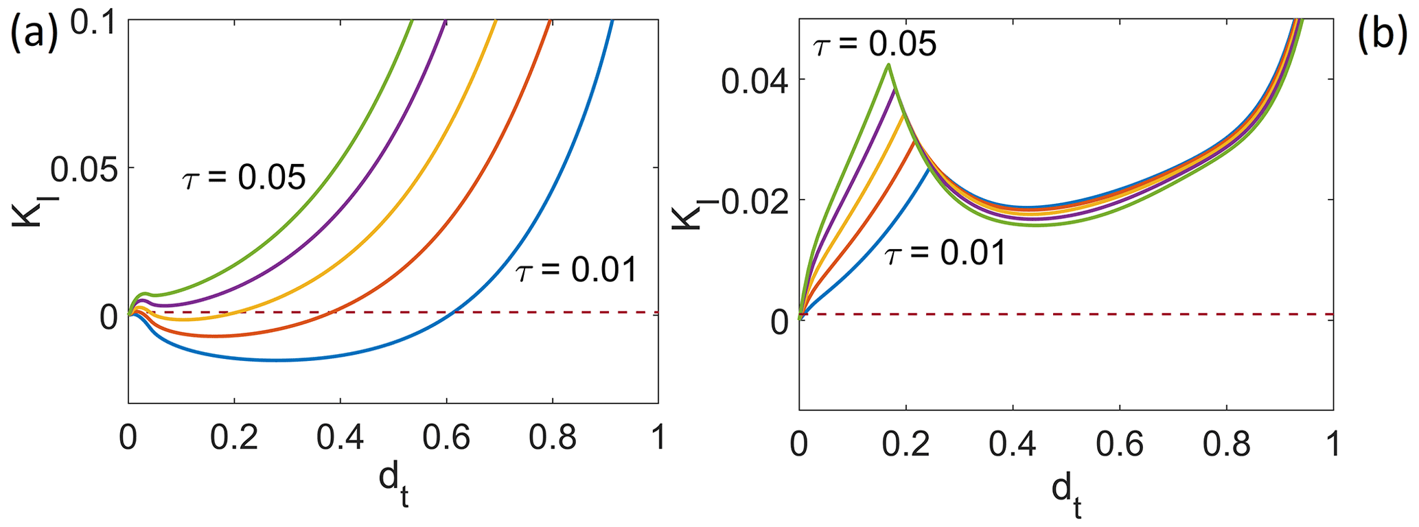
Figure 2Scaled stress intensity factor versus the crack length for different values of scaled extensional stress: τ=0.01 (blue), τ=0.02 (red), τ=0.03 (yellow), τ=0.04 (purple) and τ=0.05 (green), for (a) scaled water level depth η=0.04 and (b) scaled water volume β=0.01, without the contact condition. Fracture toughness κ=0.001 is shown as a dashed maroon line. Panel (a) is qualitatively equivalent to Fig. 10 in van der Veen (1998a) and Extended Data Fig. 5 in Lai et al. (2020).
It is straightforward to see that the main forcing parameters are dimensionless extensional stress τ, dimensionless fracture toughness κ, and either water table depth η or water volume β, treating the density ratio r as well as Poisson's ratio ν as constant. The dynamics of a single crack are simple: the crack will lengthen if the dimensionless stress intensity factor KI corresponding to crack length dt and the given forcing parameters exceeds the dimensionless critical value κ.
Consider first a crack originating at the upper surface. Figure 2 shows the dimensionless stress intensity factor as a function of surface crack length, for different values of the tensile stress parameter τ that are plausible for floating ice shelves: panel a shows curves of KI(dt) for different τ values at a fixed water table depth η=0.04 (for instance, a water level 20 m below the surface of a 500 m thick ice shelf), and panel b shows curves for a fixed scaled water volume β=0.01 (this is equivalent to around 10 m2 volume of water per unit lateral width of a 500 m thick shelf with E=109 Pa). In this figure, for consistency with van der Veen's approach (van der Veen, 1998a), we suspend application of the contact constraint in Eq. (10) and instead impose the stress conditions with an appropriate pf everywhere along the boundary. Note that we will see shortly that omitting the contact constraint has significant dynamical consequences.
In each panel, the horizontal dashed line indicates an assumed scaled value of (which corresponds to KIc=0.1 MPa m for a 500 m thick shelf). Points of intersection between the coloured curves of KI(dt) and the dashed line are steady-state crack lengths. More precisely, they are the end points of a finite region of steady states, since any crack length for which KI<κ is also a steady state. These end-point steady states are stable if at the point of intersection (so a lengthening of the crack causes the stress intensity factor to decrease) and unstable if .
We see a fundamental difference in behaviour between the fixed-water-level and fixed-water-volume cases here. For a fixed water level (Fig. 2a), we reproduce van der Veen's results (van der Veen, 1998a), at least qualitatively (there are minor differences between our models in terms of the assumed ice density): for a finite water level depth η, KI(dt) at first increases with crack length dt at a rate proportional to (see Weertman, 1980, and Appendix C) due to a dominant contribution from a constant extensional viscous pre-stress, and then it decreases due to increasing cryostatic confining stress at depth. Once the crack tip is sufficiently below the prescribed water table depth η, water pressure in the crack increases at a larger rate with dt than overburden and therefore reduces the effect of cryostatic confining pressure. The result is that there are up to three points of intersection between the coloured curves and the dashed line, where KI(dt)=κ: two shallow-crack configurations with relatively small dt values and one with large dt. The shorter of the two shallow cracks is destabilized by the extensional stress, and the second is stabilized by increasing cryostatic pressure. The third, deep-crack configuration is destabilized by water pressure increasing with depth and the effect of the torque generated by viscous pre-stress and fluid pressure becoming more concentrated as the remaining uncracked ice below the crack tip becomes thinner (see Appendix C).
Since these points of intersection between the coloured curves and the dashed line define the end points of regions of steady states, we see that for intermediate τ there are two such regions that are separate: a region of very shallow cracks, for which the stress intensity factor, dominated by extensional stress τ, is not yet large enough and a larger one in which cryostatic pressure stabilizes the crack and water pressure is not yet large enough to destabilize it. The extent of these two regions depends on the value of τ: for small τ=0.01, the two regions merge, as the extensional stress is not large enough to cause KI to rise above κ, while for τ=0.04 and above, the region of larger steady states has become extinct as cryostatic stress no longer suffices to depress KI. Importantly, Fig. 2 shows these ranges for a single water table depth η, and we will explore the dependence of steady states on η more systematically in Sect. 4.4.
For the fixed-water-volume case in Fig. 2b, the stress intensity factor KI initially increases with crack length dt, as it does for the fixed-water-level case, before decreasing again. The initial increase in KI with dt is driven by the viscous pre-stress τ and by increasing water depth in the crack driving up the fluid pressure pf near the crack tip: for small dt values, not all the prescribed water volume β can be accommodated in the crack, and the water level remains at the ice surface with η=0. Water depth and water pressure therefore increase initially with crack length dt. This ceases to be the case once the crack is long enough to accommodate the prescribed volume, at which point water level then starts to decrease with further lengthening of the crack, reducing the fluid pressure near the top of the crack and hence KI; the point where all the required water volume β is accommodated in the crack is easily identifiable by the discontinuity in in Fig. 2b.
For larger dt beyond about 0.5, KI increases again. This can be attributed to the water level dropping more slowly (that is, η increasing) with dt as the crack gets longer and the crack width is more limited due to increasing cryostatic pressure dominating the effect of the extensional stress τ. The more limited width requires a greater water column height (Fig. 3d), which (perhaps counterintuitively) leads to an increasing stress intensity factor due to the more rapid increase in water pressure pf relative to cryostatic pressure with depth.
For the chosen parameter settings in Fig. 2b, we see that there is a single range of steady-state crack lengths, at very shallow depths. As we will explore later, the dependence of KI on dt is in fact highly dependent on forcing parameters, and it is possible to generate steady states with much longer dt. Before we do so, we address the role played by contact constraints in determining KI.
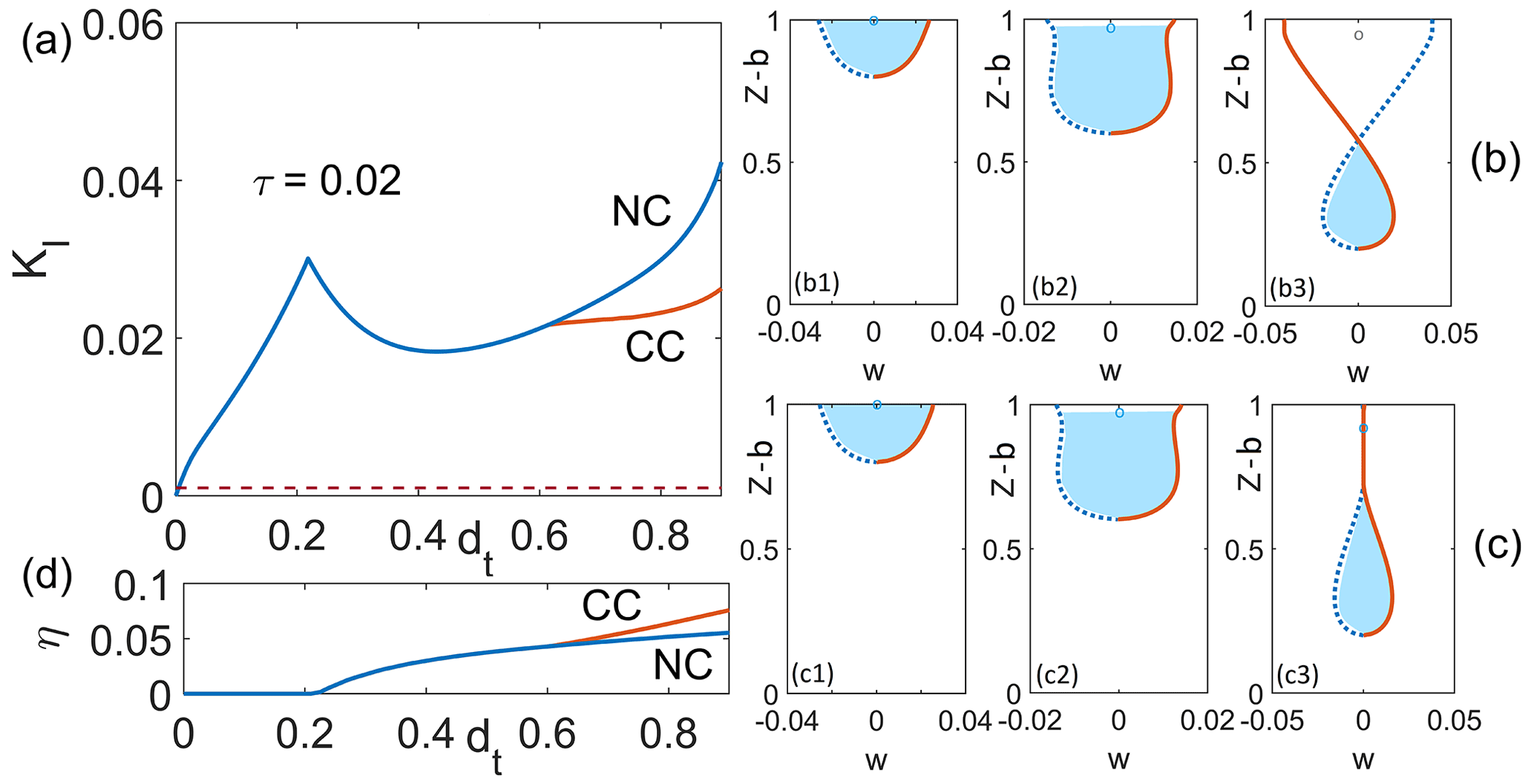
Figure 3(a) Scaled stress intensity factor KI plotted against the crack length dt for scaled water volume, β=0.01, and scaled extensional stress, τ=0.02, with (blue) and without (orange) applying the contact condition, as indicated by CC and NC, respectively. (b, c) The corresponding crack width w(z) plotted against z for dt=0.2 (b1, c1), dt=0.4 (b2, c2) and dt=0.8 (b3, c3), without (row b) and with (row c) the contact condition. The left-hand crack face is shown in dotted blue, the right in solid orange and water-filled parts of the crack in light blue. A circle indicates the “water level” (as defined by η) even where the crack is closed. Note that the horizontal axis is scaled differently in each column for clarity. (d) The corresponding water level against crack length for the case shown in panel (a).
4.2 The effect of contact constraints
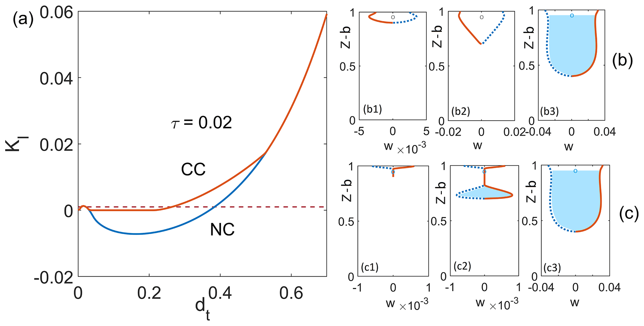
The results in Fig. 2 were computed without imposing a contact constraint. As the crack gets longer, the crack walls in the upper portion of the crack bulge inwards towards each other. Without the constraint on crack width w for the results shown in Fig. 2, in van der Veen (1998a, b), and Lai et al. (2020), the crack walls not only touch but eventually overlap at larger dt (Figs. 4b and 3b). That is, of course, aphysical. Figure 4a shows how re-introducing the constraint w≥0 affects the dependence of KI on crack length dt. The most obvious feature of the orange curve (computed with the constraint in place) is that KI no longer becomes negative: a negative stress intensity factor invariably corresponds to negative crack width near the crack tip and is therefore aphysical.
The contact constraint however does not simply amount to setting KI to zero where the unconstrained solution predicts negative KI: the two solutions can differ from each other even where both predict KI>0 (for instance in Fig. 4a for values of dt between 0.4 and 0.5). This difference occurs because contact between the crack faces can occur at higher elevations in the crack, as illustrated in Fig. 4c2. This situation raises an interesting question about the water pocket that exists below the contact area: if the water level is fixed at some depth η below the surface and the contact area is at or below that elevation, how should water pressure in the deeper water pocket be prescribed? Our model assumes that fluid pressure continues to follow a hydrostatic increase below the imposed water table depth even when the two are separated by a contact area, implying that asperities in the crack continue to provide a hydraulic connection across the contact area. That, however, is only one possible explanation, and isolated deeper water pockets (separated from the water table by a contact area) can conceivably behave as fixed water volumes instead, corresponding to the case of fixed β we consider below.
Generally, for fixed water table depth η, the effect of crack wall contact is to create a compressive normal stress greater than the fluid pressure pf that would otherwise act in the crack. Overall force and torque balance dictate that tensile stresses and torques in the unbroken portion of ice below the crack tip (for ) increase to compensate for this. This explains why the stress intensity factor increases in Fig. 4 when the contact constraint is imposed.
The effect of the contact constraint on the stress intensity factor differs for the constant volume case. With the parameter values used in Fig. 3a, KI is positive for all dt>0, no matter whether the contact constraint is applied or not. However, the solution with the contact constraint applied has a lower KI than the solution without it once a contact area forms higher up in the ice (above dt>0.6). The reason for this is that, with a contact condition, a longer water pocket (with w>0) naturally forms (Fig. 3c3 versus Fig. 3b3) and a lower water pressure (or equally, a larger η) suffices to accommodate the prescribed water volume (Fig. 3d).
4.3 Larger extensional stresses and lower water levels
Figures 2, 3 and 4 were computed for relatively small values of τ and equally for a small water depth η and water volume β, and the qualitative behaviour of KI(dt) is much the same as in van der Veen (1998a). Note that the behaviour of KI(dt) changes substantially for larger τ as shown in Fig. 5, which is computed with the contact constraint in place. In Fig. 2, there is an increase in KI with dt at small crack lengths due to the dominant action of the extensional stress τ. KI then reaches a maximum at small to moderate dt, at a point where cryostatic pressure starts to dominate normal stresses on the crack. In both panels of Fig. 2, there is a local minimum in KI, and the stress intensity factor increases again due to rising fluid pressure for cracks that span most of the ice thickness. By contrast, for larger τ, the maximum in KI is reached at significantly greater depths, and KI may or may not increase as dt→1.

Figure 5(a) Stress intensity factor versus the crack length for large-scale extensional stress, τ=0.1 (blue), τ=0.2 (orange), τ=0.3 (yellow), τ=0.4 (purple) and τ=0.5 (green) for (a) η=0.6 and (b) β=0.01, both computed with the contact constraints being satisfied.
In fact, Fig. 5 indicates that the generic behaviour for a crack that spans nearly the full ice thickness is that either KI=0 or as dt→1. This can be attributed to the torques generated by extensional stress τ, cryostatic pressure s−z and fluid pressure pf (or contact stress in the contact areas) on the remnant “neck” of ice that still connects the two sides of the domain, with a singular KI favoured by smaller water level depth η. We explain this in greater detail in Appendix C, where we show how it is often possible to determine the critical combination of parameter values at which the change in KI from zero to infinite occurs.
As in Sect. 4.1, we can read steady-state ranges off these plots by identifying where KI<κ. For the fixed-water-level case, we see that there is still a short region of shallow steady-state cracks near dt=0 and potentially a region of much larger steady states. Whether that latter region exists and whether it extends all the way to dt=1 or terminates at an unstable steady state depend on parameters: for smaller η and τ, we still obtain a region of steady states that terminates short of the full ice thickness dt=1, while for larger τ, we obtain either a region that extends to dt if η is sufficiently large (that is, water pressure is lower) or no region at all at smaller η (higher water pressure). Note that either an increase in τ or a reduction in η always shrinks the region of steady states, as might be expected on physical grounds.
For a fixed water volume, we see a region of larger steady states appear at intermediate values of τ where there was none for small τ (Fig. 5b). The appearance of these steady states corresponds to the plots KI(dt) for τ=0.2 and τ=0.3 having KI=0 and lying below the curve for τ=0.1 at larger dt values in Fig. 5b. This is a major difference between the two hydrology models, since increased τ invariably reduces the range of steady states for the fixed-water-level case. Physically, the behaviour for a fixed water volume β can be explained by larger extensional stress opening the crack further, so the prescribed water volume can be accommodated lower down in the ice column, leading to reduced fluid pressure and therefore to lower KI.
4.4 Dependence of steady states on parameters
We have so far focused on identifying steady states for discrete parameter values of τ and η as shown in Fig. 4 (or Fig. 2 if we ignore the contact constraint) and Fig. 5. Instead, we can also plot the boundaries of the region of steady states explicitly as functions of the model parameters: such a plot is effectively a bifurcation diagram for the semi-smooth dynamical system defined by Eq. (20).
Figure 6a and b show an example for a number of fixed-water-level values, using the dimensionless extensional stress τ as the parameter being varied. The area to the left of each curve (shaded in light grey for η=0.06 in panel a and for η=0.2 in panel b) represents steady-state values of dt for the corresponding τ. The boundary curves of these areas are computed by solving for KI=κ using a continuation method, with KI computed from the model with the contact constraint enabled. A dashed portion of the boundary curve corresponds to an unstable boundary as defined above and a solid curve to a stable boundary. Outside of the steady-state regions, dt invariably increases with time (since, by construction, crack length cannot shrink).
The results in Fig. 6a and b correspond to the observations we have made previously based on Figs. 4 and 5a: in panel a, we see the split of the steady-state area into two separate parts at relatively small τ and η. The lower region (near dt=0) once more represents very shallow steady-state cracks. This regions thins progressively with increasing τ as τ−2 (since on the dashed upper boundary of this lower region; see Appendix C) but never disappears entirely: provided an initial crack is shallow enough, it may never grow at all.
Note that the upper boundary of this lower region is insensitive to water level η. The lower dashed boundary curve may appear to exist only for η=1 as indicated by the maroon curve. That is however simply the result of the boundary curves for different water level values being indistinguishable. In most cases, they coincide exactly because they correspond to dry cracks with dt<η. The case η=0 (a completely full surface crevasse) is something of an exception: here dt>η everywhere and the boundary curve is not identical to the others but close enough almost everywhere to be indistinguishable as KI is dominated by the effects of the pre-stress τ. By contrast, with the case of non-zero water level depth, there is also no split into a lower and an upper steady-state region for η=0; only the narrow band of shallow steady states exists. Note that this reproduces the results in Lai et al. (2020) and in particular the corresponding curves for water-filled crevasses in Fig. 5c and d of the Supplement to Lai et al. (2020).
For non-zero water level depth η, there is often an upper region consisting of steady cracks of more substantial size. This region is enlarged for a fixed extensional stress τ if the water level drops (η increases) and shrinks if τ is increased for fixed η. In fact, the upper region only exists conditionally, for sufficiently small τ (given η) or sufficiently large η (given τ). This is to be expected: high water levels (small η) or large extensional stresses τ will destabilize large cracks and cause them to propagate all the way through the ice.
In greater detail, depending on η, there are two possible configurations for the upper region of steady states and two possible ways in which it shrinks and eventually disappears as τ is increased at fixed η. At small to moderate η, the larger range of steady states lies between a stable lower boundary (marked by a solid line) and an unstable upper boundary (dashed line), with the two meeting at a turning point for some critical value of τ; this turning point corresponds to a so-called saddle-node bifurcation of the dynamical system (20) (albeit a somewhat unusual one because the system is semi-smooth, and the entire region between the unstable upper and stable lower curve consists of steady states).
By contrast, for sufficiently low water levels (large η), the upper region of steady states lies between a stable lower boundary (solid line) and the maximum possible crack length of dt=1 as the upper boundary: arbitrarily thin necks of ice (with dt arbitrarily close to the full ice thickness value of 1) can remain in steady state. As τ increases, the lower boundary simply approaches dt=1 smoothly, and the upper region of steady states disappears when the two meet at finite τ (see Appendix C).
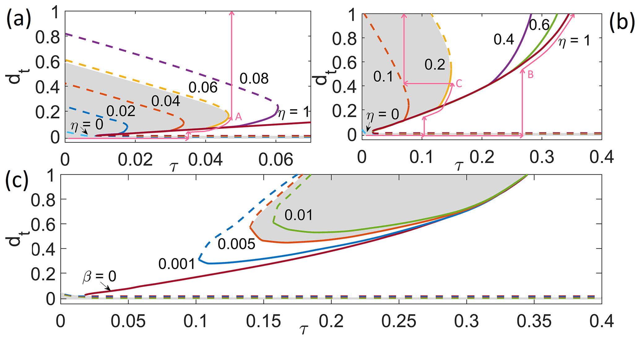
Figure 6Bifurcation diagram with contact condition, for an ice shelf with a single crack at the top. Each heavy solid or dashed curve is the locus of points satisfying or in the (τ,dt) plane at a fixed value of η or β as indicated, representing the boundary of a region of steady states in which K1≤κ. A solid portion of the boundary curve indicates a stable boundary, and dashed indicates unstable. (a, b) The case of constant η, the value of η being indicated for each curve. The region of steady states generally lies to the left of each curve, as indicated by grey shading for η=0.06 (panel a) and η=0.2 (panel b). The two panels differ in the range of τ and η. Note that there is a narrow region of steady states near dt=0 in each panel (elevated slightly above the bottom of the plot for visibility). Also shown as narrow pink curves are three phase paths that the point (τ,dt) can follow under changes in τ and η. All paths begin at a small dt and τ=0; paths A and B correspond to monotonic increases in τ at different fixed values of η= 0.06 (A) and 1 (B). Path C corresponds to a monotonic increase and subsequent decrease in τ at η=0.2 followed by τ being held fixed while η is lowered to 0.1. (c) The case of constant β, values as indicated and steady-state region indicated for β=0.005 using the same plotting scheme as panels (a) and (b). Note that there is again a narrow region of steady states near dt=0.
The constant-water-volume case differs considerably from the constant-water-level case. In Fig. 6c, we show an analogous bifurcation diagram for the system at different fixed values of β, with τ again being the parameter allowed to vary continuously. As already deduced from Figs. 3 and 5b, we see again a narrow region of steady states close to dt=0 (shaded in grey, with a dashed, unstable upper boundary). For non-zero water volume β, the boundary curve of that region is in fact identical to that for η=0, since these solutions correspond to full surface cracks that are unable to accommodate all of the prescribed water volume.
For a non-zero water volume, an upper region of steady states does appear (shaded in grey for β=0.005) but only above some critical τ: as previously discussed, the opening of the crevasse at larger extensional pre-stress allows the prescribed water volume to be accommodated at greater depths, leading to perhaps counterintuitively reduced stress intensity factor values KI. The larger the prescribed water value, the smaller the upper region of steady states becomes, and the values of τ at which we find the upper region generally exceed the range that is typically expected for ice shelves. For completeness, note that the upper region of steady states becomes much more extensive as water volume β shrinks: the case β=0 (a dry crack) becomes identical to the dry-crack case η=1 in Fig. 6b.
The work above has focused on surface cracks. The case of a single basal crack (van der Veen, 1998b) is in fact simpler than the surface crack, since there is no hydrological parameter β or η to take care of. The dependence of KI on crack length db is again shown in Fig. 7. Note that contact areas never form lower in the crack but are always adjacent to the crack tip (Fig. 8a), and the effect of introducing the contact constraint is simply to truncate KI computed from the model without a contact constraint at zero (compare Fig. 7a and b). As in Fig. 5, we see a pattern of KI increasing from KI=0 at db=0. For τ less than a numerically determined critical value of τcrit=0.039, KI then decreases again and vanishes for db close to unity, while for τ above this value, KI diverges to +∞ as db→1 (see Fig. 8c); this can again be attributed to the torque exerted on the narrowing neck of ice connecting the two halves of the domain as described in Appendix C: there we show that the critical value for τ at which this occurs can in fact be explained by the torque changing signs, with a theoretical calculation giving a value of . We attribute the difference between the value to the difficulty in computing stresses accurately at finite element sizes when the remnant neck of ice is shrunk towards zero size.
The resulting dependence of the region of steady states on the parameter τ is shown in Fig. 8b: as for the surface crack, there is always a narrow range of shallow steady states near db=0 and generally a larger range of steady states extending all the way to db=1 (corresponding to full crack penetration). That latter range becomes narrower and vanishes at the critical τ=0.039. Because that vanishing corresponds to the behaviour of KI near dt flipping from KI=0 ( when there is no contact condition) to , the critical value is independent of κ. Note that the same result is implicit in Fig. 4c of the Extended Data in Lai et al. (2020), where complete penetration of a basal crack is also displaced as occurring at a fixed value of τ close to 0.039.
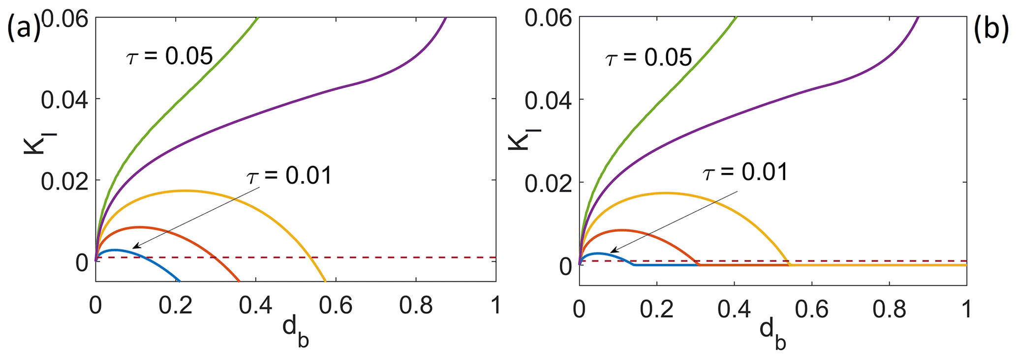
Figure 7(a) Stress intensity factor against crack length for a basal crack for different values of τ (same plotting scheme as Fig. 2, without (a) and with (b) contact conditions. Panel (a) is qualitatively equivalent to Fig. 2 in van der Veen (1998b).
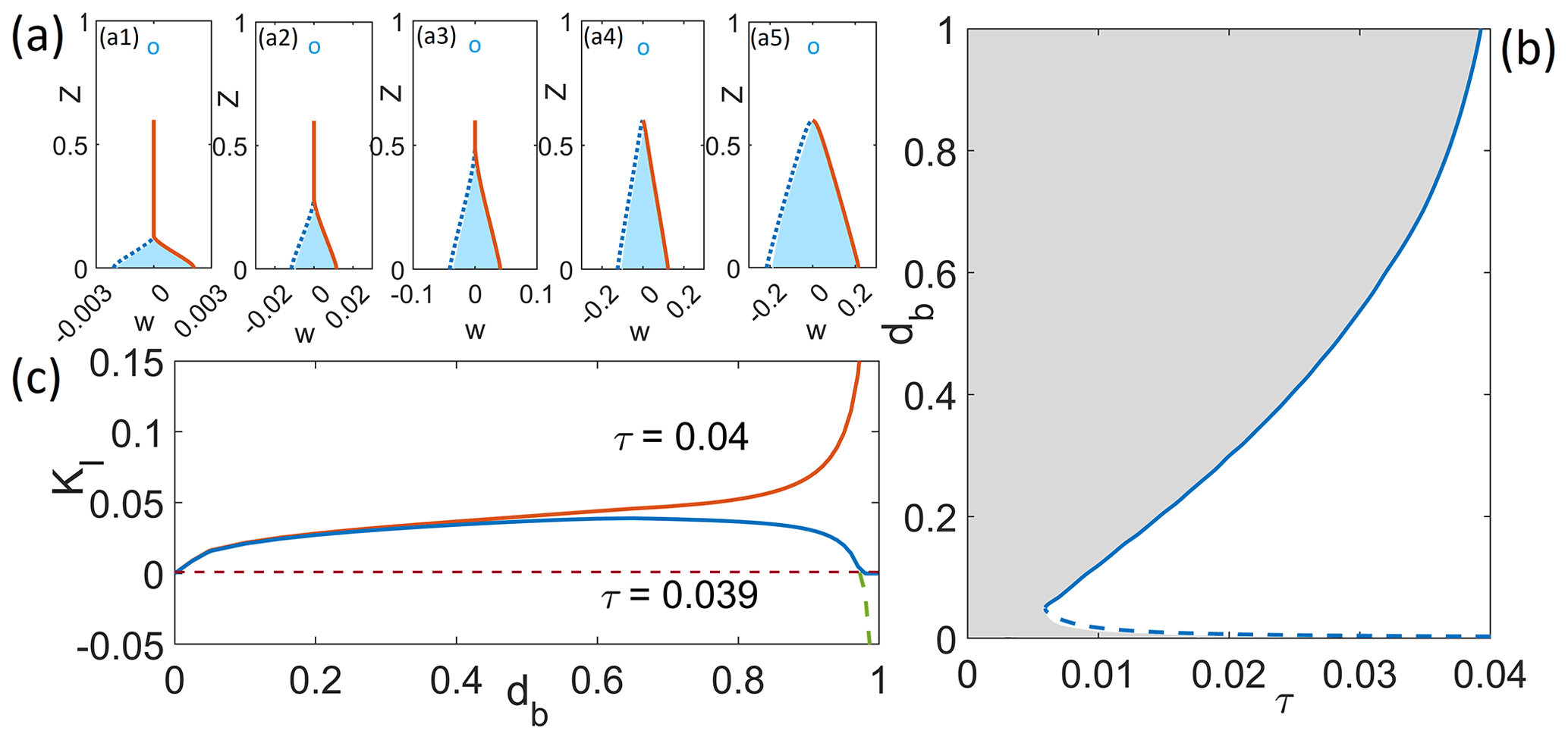
Figure 8(a) Crack opening w(z) computed with the contact condition, at db=0.6 for τ=0.01 (a1), τ=0.02 (a2), τ=0.03 (a3), τ=0.04 (a4) and τ=0.05 (a5), with the same plotting scheme as Fig. 3c; water level as indicated by the circle is sea level. (b) Bifurcation diagram for the basal crack for κ=0.001, with the same plotting scheme as Fig. 6 except that there is now a single boundary curve since there is no hydrological parameter. (c) Stress intensity factor versus basal crack length for τ=0.039 and τ=0.04. The dashed green line shows the result for τ=0.039 without the contact condition. Calving occurs when KI changes (under changes in τ from being zero to diverging to +∞ near db=1) and is independent of the stress intensity factor as a result.
4.5 Calving
We can understand calving as the formation of a crack that spans the entire thickness of the ice as the result of a change in the forcing applied to the ice shelf. In order to make sense of that using only the model in the present paper, we have to assume not only that we can use the parameters τ, η and κ to represent changes in forcing but also that we can ignore changes in the specific form of pre-stress given in Eq. (24) (through which τ is ultimately defined) as well as changes in the local ice shelf geometry into which a new crack is incised or in which an existing crack is lengthened. These assumptions of course do not hold in practice: viscous pre-stress evolves over a single Maxwell time (given by the ratio of ice viscosity to Young's modulus, typically hours to a day for a polar ice shelf) once an initial crack has formed, and pre-stress will not remain of the form in Eq. (24). Secondly, the local geometry of the ice shelf will also evolve, although more slowly, once a partial crack (which does not span the entire ice thickness) has been incised (Yu et al., 2017).
It is however instructive to pursue the evolution of cracks as described by our model alone under changes in parameters, leaving the evolution of viscous pre-stress and geometry to future work. Doing so allows us to develop a framework for understanding calving. Under the assumptions we are making, the parameters τ, η and κ can be expected to evolve slowly compared with the dynamic crack propagation timescale. That timescale is inertial in our model, but the same would be true if we were to use a hydrofracture model with a dynamically evolving crack fluid pressure field pf (Spence and Sharpe, 1985). The stress parameter τ represents deviatoric stresses in the ice and evolves as the large-scale ice geometry does (over many years due to ice flow, unless there is another calving event happening elsewhere in the shelf), while water level η is likely to evolve seasonally. The scaled fracture toughness κ invariably changes slowly: with fixed KIc, κ changes purely because ice thickness evolves.
Following the discussion above, consider an example of how slow changes in the parameter τ can lead to calving. In Fig. 6a, the point (τ,dt) is a possible steady-state crack configuration for given (η,κ) if it is inside the region of steady states or if it is on a solid (stable) part of the boundary. If the point lies initially inside the steady-state region rather than on its boundary, then the value of dt will not change as a result of a parameter change: under a change in τ, the point in question moves horizontally (parallel to the τ axis). Suppose the point reaches a stable part of the boundary under such a change in τ (that change being, invariably, an increase). Then any further increase in τ would take (τ,dt) outside of the steady-state region if dt were to remain unchanged. Of course, instead of exiting the steady-state region, (τ,dt) will simply follow the stable boundary while this is possible.
By contrast, if the point reaches the end of the stable part of the boundary (as it does at the saddle-node bifurcation in Fig. 6), if the point otherwise reaches an unstable part of the boundary of the shaded region (as is possible under changes in τ with the right initial crack length dt) or if it starts outside the region altogether, then dt will increase rapidly while the parameter value τ remains essentially constant (since we assume that forcing changes on much longer timescales than that associated with crack propagation). In other words, the point (τ,dt) moves vertically in the bifurcation diagram, parallel to the dt axis. It will continue to move in that direction until it hits a stable boundary of a region of steady states (which is possible if the crack starts in the narrow region of shallow steady states and transitions to a separate region of larger steady states above) or until it hits the line dt=1 and the domain is severed. The latter represents a calving event (as illustrated by path A in Fig. 6a). Here, crack length does not continuously grow to span the entire ice thickness but becomes unstable and rapidly propagates the remaining ice thickness.
An alternative calving mechanism for lower water levels (larger η) is that there is no saddle-node bifurcation, and the stable boundary of the region of steady states smoothly approaches dt=1 under increases in τ (see Fig. 6b for η=0.4, η=0.6 and η=1). Calving in this fashion simply involves crack length growing continuously until the last remaining neck of ice is severed (see path B in Fig. 6b), although this requires not only low water levels but also unrealistically larger extensional stresses for the surface cracks in Fig. 6b (recall once more that in an unconfined ice shelf, τ≈0.05, and we expect lower extensional stresses in typical buttressed ice shelves).
Calving can also occur through changes in η, κ or multiple parameters at once. At fixed τ, calving due to decreases in η can occur in a similar fashion to calving due to increases in τ: either through reaching a saddle-node bifurcation or the unstable boundary of the upper region of steady states for small to moderate τ or through the stable lower boundary of that upper region smoothly reaching dt=1. Combined changes in τ and η can further complicate the style of calving and make it more likely that calving occurs by reaching the unstable upper boundary of the upper region of steady states as illustrated in Fig. 6a: in particular a temporary increase in τ that does not in itself induce calving may still lengthen the crack appreciably, which a subsequent reduction in τ does not then reverse. If η is reduced later (that is, the water level rises), the previously lengthened crack may become unstable and cause calving even if the initially much shorter crack would not be susceptible to calving at the same combination of (τ,η) (see path C in Fig. 6b).
As discussed at the end of the previous section, the calving mechanism for bottom cracks is analogous to the second mechanism for surface cracks described above: calving occurs when the stable upper branch of the boundary curve of the stable region in Fig. 8b reaches dt=1.
For the fixed-water-volume case, the situation appears to be quite different: for most of the water volume values in Fig. 6c, except for exotic initial conditions, calving at realistic values of extensional stress τ appears to occur whenever (τ,dt) hits the unstable boundary of the lower region of steady states, consisting of very shallow cracks. It seems implausible that limited amounts of water should cause calving at low stress but not at high stress. We discuss this further in Sect. 6, where we argue that Fig. 6c may in fact be a red herring as a description of calving if viewed in a three-dimensional geometry.
A calving law is a parameterization of calving that can be used in a large-scale ice sheet model. Ideally, we would like something like a relationship between the different model parameters. For the case of a bottom crack propagating upwards, the results at the end of Sect. 4.4 (see Fig. 8) in fact furnish a calving law, of the very simple form
since the critical value τcrit does not depend on scaled fracture toughness and there is no hydrological parameter to take care of. Numerically, we have found τcrit=0.039, while theory (Appendix C) predicts a slightly lower value of τcrit=0.0367. An analogous result is shown in Fig. 4c of the Extended Data in Lai et al. (2020).
For a prescribed surface water level, an equivalent relationship would take the form , at which calving happens in the sense of dt rapidly transitioning to a value of 1 when that relationship is satisfied or reaching unity continuously. If there were such a relationship, then using the definition of τ, η and κ, calving for a surface crack with a fixed water level would occur when
An equation of the form (36) can be implemented in a large-scale ice sheet model where thickness and stress are dynamical variables, and a surface hydrology model could conceivably be developed to predict water level hw. In fact, structurally, these calving laws are analogous to others such as that in Nick et al. (2010) and Schoof et al. (2017), in which calving happens at a critical thickness H that depends on extensional stress and a hydrological parameter analogous to hw: Eq. (36) defines an implicit relationship between H and the remaining model parameters.
The problem is however that there is no unique function ft, in general. To understand why this is so, recall our discussion in Sect. 4.5 of the sample phase paths (Fig. 6): take for instance path C, which leads to calving through reaching the unstable upper boundary of the upper region of steady states at a combination of (τ,η) for a crack that has not been lengthened and previously would remain steady. There is no unique calving behaviour even in the simple set-up considered here, and calving is strongly history-dependent: cracks that were lengthened previously (by parameter changes that were subsequently reversed) favour earlier calving.
In principle, we have a recipe for computing the trajectory of dt in phase space in response to slow changes in parameters : if T is a slow time variable associated with large-scale evolution of the ice shelf, then the current crack length dt(T) can be computed in terms of the “most recent” crack length and the set of stable steady states S, defined through , where sup and inf (below) are the usual lowest upper bound and greatest lower bound, and we include the “calved” solution dt=1 in the set of stable steady states. In this notation, we have
and calving occurs when dt first reaches unity.
This is clumsy-looking but possible to implement numerically in a dynamical ice sheet model if the set S is known a priori from offline computations such as those shown in Fig. 6. We can construct a simpler description of calving, of the form in Eq. (36), if we assume that crack length will always track the stable lower boundary of the upper region of steady states in Fig. 6, whenever that boundary exists. Within our model, this occurs principally if τ never decreases in time and η never increases in time; alternatively, we can assume that the crevasse will heal rapidly (relative to the timescale over which the forcing parameters change), resetting dt to the nearest shorter length at which KI is equal to the fracture toughness κ.
If crack length is forced in this way to follow that lower boundary whenever possible, then calving occurs either because the lower boundary terminates at a saddle-node bifurcation or because it reaches the maximum possible crack length dt=1. The location of the bifurcation or of the point at which the stable lower boundary reaches dt=1 defines τ as a function of κ and η. More generally, it defines a surface in space as in Eq. (36). As an example, Fig. 9 shows τ at calving as a function of η for the fixed values of κ=0 to 0.01. Note that the curves corresponding to different κ values differ primarily through their starting points as shown in the inset figure: the saddle-node bifurcation first appears at some finite τ, which corresponds to the split into the lower and upper regions of steady states in Fig. 6a, and that starting point depends on κ. For larger water depths η, calving becomes insensitive to the scaled fracture toughness.
In fact, for combinations of sufficiently large τ and η, calving occurs through the continuous shrinking of the neck of ice of thickness 1−dt as stress increases or water depth η decreases, and calving is controlled by torques on that neck of ice. Appendix C furnishes an asymptotic form for ft in that case, of the form
valid for τ close to a critical value of one-third. This form of the calving law is plotted as a dashed line in Fig. 9: it turns out that it captures the calving law quite well for a relatively large range of τ. As in the case of bottom cracks (see the end of Sect. 4.5), we find that theory and numerical results do not agree perfectly even where the theoretical result is expected to be accurate (near , η=1). We attribute that once more to the difficulty in computing KI accurately using finite-sized boundary elements when the ice neck thickness 1−dt shrinks to zero.
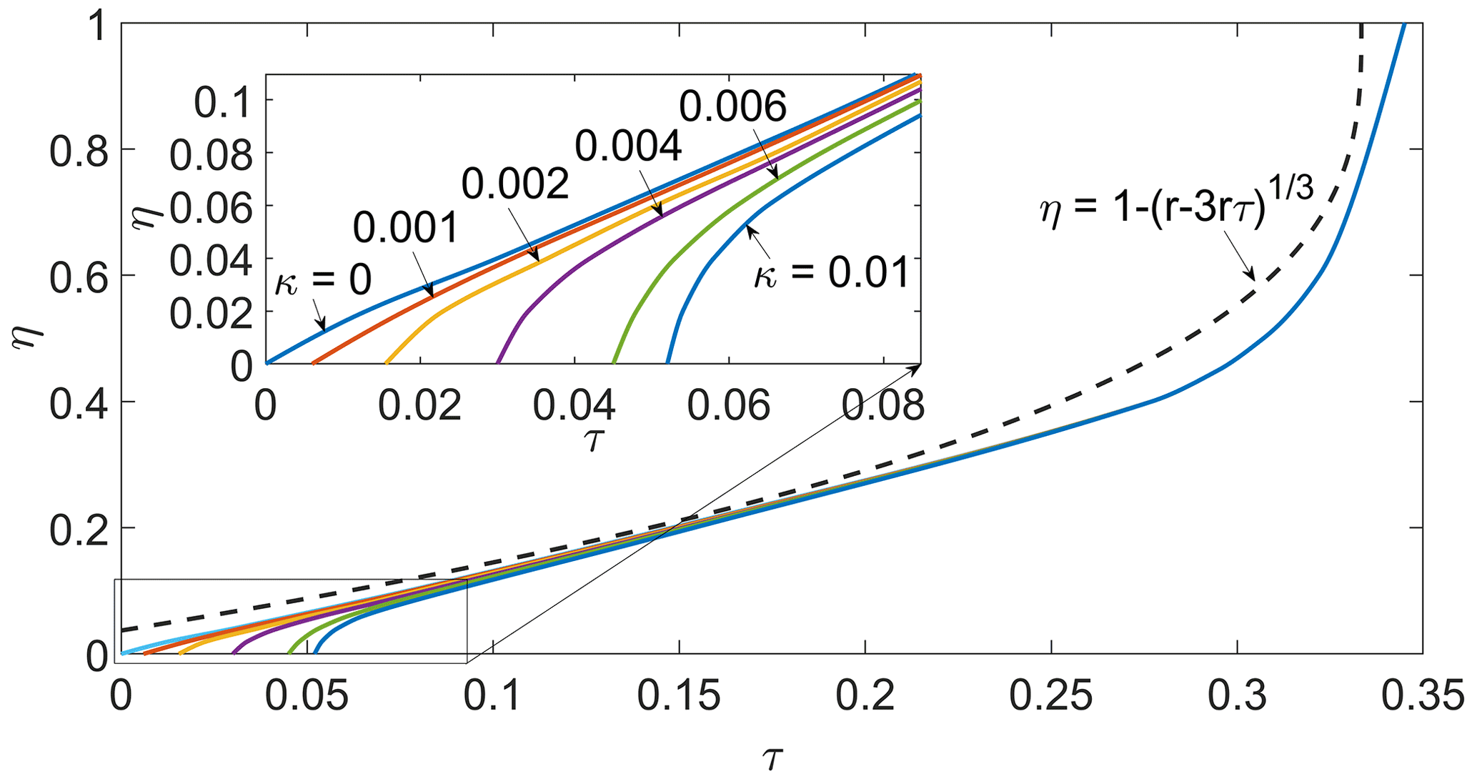
Figure 9The location of the saddle-node bifurcation point in Fig. 6 (if it exists) or the location where the boundary reaches dt=1 when there is no saddle-node bifurcation, plotted as τ at the bifurcation point against the corresponding η, for different values of scaled fracture toughness, κ. An enlargement of the bottom left-hand corner identifying the colour scheme is shown at top left. The dashed curve represents the analytical calving law in Eq. (38).
As discussed at the end of Sect. 4.5, the finite water volume case does not offer any obvious path to a calving law: fracture propagation can be expected to occur across the full ice thickness for realistic values of τ once (τ,dt) reaches the unstable upper boundary of the lower region of steady states in Fig. 6c and is as such heavily dependent on initial conditions. We expect no equivalent to Eq. (36) in that case. What is more, however, is that it also remains unclear whether that complete fracture propagation would necessarily correspond to calving or perhaps instead simply to the drainage of the prescribed water volume through a localized slot that reaches the bottom of the ice shelf. We return to this shortly below.
In this paper, we have extended the two-dimensional theory for penetration of partially water-filled crevasses in an ice shelf by linear elastic fracture mechanics as developed previously by van der Veen (1998a, b) and Lai et al. (2020); as in these papers, the situation we have in mind is a crevasse that is distant from either the grounding line or the calving front (see also Hooke and Hanson, 2017; Wagner et al., 2016). We have explicitly formulated the crevasse penetration problem in terms of a viscous pre-stress and an elastic stress induced by the sudden introduction of a crack (see also Yu et al., 2017). The mathematical form of the problem for a domain in the shape of a parallel-sided slab prior to crack penetration is identical to that in van der Veen (1998a, b) and Lai et al. (2020) except for the addition of contact constraints. Owing to a solution method based on interpolated Green's functions being used in van der Veen (1998a, b) and Lai et al. (2020), these authors are not able to prevent crack faces from intersecting each other aphysically when a crack opening becomes negative. We are able to rectify that by modifying the standard displacement discontinuity boundary element method (Crouch and Starfield, 1983), applicable to arbitrary domain shapes, to account for contact constraints and solve for the crack tip stress intensity factor and crack propagation rate (Sect. 3 and Appendix B), based on a quasi-static crack propagation description due to Freund (1990).
The focus of our paper is to determine conditions under which a crack is able to propagate across the entire thickness of the ice, which we interpret as a calving event. While van der Veen (1998a, b), using a nearly identical basic fracture mechanics model (omitting only the contact constraints), largely stopped short of identifying conditions for calving this way, Lai et al. (2020) do so for a single surface crack that is either completely dry or completely filled with water. Here, we extend their work to allow for a more general prescription of hydrology: we consider either a water level at a prescribed depth below the ice surface as in van der Veen (1998a) (mimicking a water table in an englacial drainage system) or a prescribed, fixed water volume in the crack as a more physics-based generalization of the fixed water column height above crack tips considered by Nick et al. (2010).
6.1 Surface cracks with a fixed water table
We show that, for surface cracks with a fixed water level below the ice surface, we generally find that very shallow cracks are in steady state but become unstable once they reach a stress-dependent critical value that is a small fraction of the ice thickness (Weertman, 1980; Lai et al., 2020). Once that occurs, two scenarios are possible: first the crack may continue to grow rapidly until it spans the entire ice thickness and calving occurs; as one would expect, this is favoured by large extensional stresses () and high water tables (small water table depths below the ice surface). Alternatively, crack growth may be arrested when crack length reaches the lower boundary of an extended region of steady states. The existence of that region of steady states is conditional on stress τ not being too large and water table depth η not being too small.
The subsequent evolution of such a partial crack under changes in forcing parameters is more complicated. If the water level is fixed and stress τ is increased, the crack length will increase continuously in τ either until the crack spans the entire ice thickness (which occurs at larger water table depths η; see phase path B in Fig. 6) or until the range of steady states disappears with the crack tip still at a finite distance from the base of the ice shelf, leading once more to rapid crack propagation and calving (which occurs for smaller water table depths η; see phase path A in Fig. 6). In either case, we can identify a critical stress τ as a function of η (or vice versa) at which calving occurs, as shown in Fig. 9; that relationship can then, in principle, be used as a calving law.
Under more general parameter changes, calving may not be as simple: for instance, a reduction in extensional stress τ will generally leave a crack that is longer than cracks that would form anew at the new, lower extensional stress, and such an overextended crack is then more susceptible to calving if the water table subsequently rises (η is reduced; see path C in Fig. 6). This observation underlines that calving is generally history-dependent, and a simple calving law relating a critical extensional stress to ice thickness and water depth (e.g. Schoof et al., 2017) cannot in general be found; instead a more complicated dynamic description of crack evolution (Eq. 37) becomes necessary.
Even if we accept the notion of a simple calving law like the parameterization in Eq. (38), we still have to contend with the question of how to determine water table depth, which becomes key in determining the stability of the ice shelf. In dimensional terms, Eq. (38) can be written in the form
at calving, with smaller values of extensional stress permitting the ice shelf to remain. Consider then the situation close to an ice shelf front, where Rxx is given by Eq. (25). Consider the case of a constant depth to the water table hw, and assume that ice thickness H increases upstream of the shelf front. Suppose that the ice shelf front is at the point of calving; that is, Eq. (39) is satisfied. We can ask what happens when calving occurs, in which case H at the new calving front position must increase. It is however easy to show that the left-hand side of Eq. (39) with Rxx given by Eq. (25) increases faster with H than the right-hand side if the constant hw lies in the physically required range .
The result is that, once the critical value of Rxx for calving is reached at the ice front, then the resulting retreat of the ice front will lead to Rxx exceeding the critical stress given by Eq. (39) and presumably continued, rapid calving. That conclusion is however entirely dependent on the prescription of a fixed water depth hw and in reality points to the need for a more refined surface hydrology model.
6.2 Surface cracks with fixed water volume
As an alternative to a fixed water table, we consider the case of a fixed water volume injected into a crack. This leads to qualitatively very different results: again there is a range of shallow steady-state cracks that become destabilized once a stress-dependent critical value is reached. Unlike the case of a fixed water level, the subsequent rapid growth of the crack is generally not arrested at low extensional stresses until the crack spans the entire ice thickness. Counterintuitively, the crack may stop growing partway across the ice only if the extensional stress is large enough (Fig. 6c): this occurs because a larger extensional stress corresponds to a wider crack, and hence the same water volume corresponds to a lower water level (and therefore water pressure).
While it may be tempting to conclude that injection of fixed water volumes invariably leads to calving if the initial crack is long enough, this may not be so: if the model were extended into the third dimension, crack propagation forced by a fixed water volume is likely not to cause the crack tip to advance uniformly but to drive a fingering instability that leads to the crack propagating all the way to the lower boundary only locally, allowing water to drain out without causing the crack to reach the lower ice boundary everywhere and therefore without causing calving (Touvet et al., 2011; Peirce, 2016). Such a fingering instability is driven by the larger water pressure in locations where the crack has already propagated further. A similar instability could occur where fracture propagation is driven by a fixed water level, but this is unlikely to stop the crack propagating completely where it has advanced less far as in the fixed volume case of Touvet et al. (2011): in the fixed volume case, the water level drops when the crack tip advances unevenly, potentially reducing the stress intensity factor in those areas where the crack tip has not propagated as far, leaving them stranded in the sense of not advancing further; for the fixed-water-level case, this does not happen.
6.3 Basal cracks
Perhaps the most important insight into the model however comes from the case of a single basal crevasse, previously considered by van der Veen (1998b) and in the Extended Data of Lai et al. (2020, their Fig. 4c). As in Lai et al. (2020), we find that basal cracks propagate across the entire ice thickness at a critical value of , regardless of the scaled stress intensity factor. Computationally, we find a critical value of Rxx=0.039ρigH, while a purely theoretical argument (Appendix C) puts the critical value at Rxx=0.0367ρigH. This is however a problem: the boundary condition on extensional stress at an ice shelf front is Rxx=0.05ρigH, implying that the stress there is necessarily above the critical value, and calving must occur provided small cracks are present to initiate crevasse growth.
Obviously, real ice shelves are known to persist for long periods of time, and there must be an issue with the model used here, in van der Veen (1998a, b) and in Lai et al. (2020). A closer look at the mechanism by which calving through the growth of basal cracks occurs in the model is required. Ultimately, calving occurs as the result of torques generated on the crack faces as described in Appendix C. If the net torque on the crack faces acts to open the crack, then it must be balanced by torques on the remaining neck of ice above the crack. As the crack length approaches the ice thickness, the neck of ice becomes very small and torque balance requires that the stresses in the neck of ice become very large and so too the stress intensity factor. In other words, with a narrow neck of ice, a net torque acting to open the crack will necessarily lead to calving.
The balance of torques we have just described however results from the zero-stress boundary conditions imposed at the sides of our domain. Here, the lack of representation of buoyancy effects in our model becomes relevant. In reality, the far field in our model is a “matching region” with a buoyantly supported thin elastic beam, which can support torques and shear forces (Sayag and Worster, 2011; Wagner et al., 2016; Warburton et al., 2020). In such a thin plate, vertical displacements cause a non-negligible imbalance between the gravitational force on an ice column and the water pressure that must be balanced by a gradient in shear force; at the ice thickness scale described by our model, such buoyancy effects are absent (see also Buck and Lai, 2021).
As Fig. 10 shows, solutions to the model used here typically correspond to solutions with non-zero vertical displacement gradients (that is, with a definite tilt) in the far field, causing the ice to emerge progressively from the water in the far field (as shown) or be submerged progressively. The adjacent beam-like part of the shelf will therefore be subject to buoyancy effects as described above. It is realistic to expect that these, in turn, will lead to far-field stresses imposed on the domain considered in our model, which cannot be uncoupled from the elastic beam region, and these stresses are likely to generate a torque that may stabilize the crack against the torque-driven calving at low extensional stresses Rxx that our model without far-field stresses currently predicts. We leave the problem of coupling the domain considered here to a beam-like far field to future work.

Figure 10The extensional stress σxx distribution for a basal crack with τ=0.06 and db=0.9. We illustrate the results here using a deformed domain, plotting σxx against a rendering of Eulerian position , where we use c=0.02 for clarity (in reality, actual displacements are smaller, with for H=500 m and Pa).
There are additional improvements to our model that need to be addressed by future work. The crack propagation rate in our model is based on a quasi-static crack propagation description due to Freund (1990). The latter most likely ought to be replaced by a hydrofracture-type description of fracture propagation (Spence and Sharpe, 1985; Tsai and Rice, 2012) in future work, in which the rate of crack propagation is controlled by changes in water pressure that occur as the crack expands and water has to flow to fill the expanded crack. For the case of a single crack propagating through the ice, the distinction between the two formulations is however moot: in either case, the crack will grow if the statically computed stress intensity factor exceeds the fracture toughness of ice (Zehnder, 2012; van der Veen, 1998a, b; Lai et al., 2020).
More significantly, the computations reported in this paper rely on a particularly simple form of the viscous pre-stress and a prescribed, parallel-sided slab geometry into which cracks are incised. Once there is a crack across part of the ice thickness, neither assumption will remain valid: elastic stresses will decay relatively quickly after crack propagation (over the Maxwell timescale), leading to an adjustment in the viscous pre-stress to ensure continued force balance, while ice geometry will adjust more slowly over an advective timescale, comparable with the time ice takes to traverse the ice shelf. The adjustment in viscous pre-stress and in ice geometry requires coupling the model for crack propagation described here with a model for viscous flow (see also Yu et al., 2017).
Assume that ice can be treated as an elastically compressible, upper-convected Maxwell fluid, with a rheology of the form
where η is viscosity, vi is velocity,
is the usual strain rate, and the superscript ▿ denotes the upper-convected derivative
Consider an abrupt change in stress due to introduction of a crack over a timescale much shorter than the Maxwell time . Assuming that strains that occur over this timescale remain small, an abrupt change in stress translates into a large derivative , with the left-hand side of Eq. (A1) dominated by the time derivative. Equation (A1) can then be approximated by
Integrating from an initial time ti at which the crack starts propagating (so σij(x,ti) is the pre-existing stress before introduction of the crack),
If the strain accumulated over the interval (ti,tf) is small, then the integral at fixed x is approximately the displacement of a Lagrangian particle at initial position x. In that case, the time integral over the strain rate simply becomes the linearized strain
accumulated over the time period in question. Hence we can write
where is the pre-stress (related viscously to the velocity field vi(x,ti) that was present before the introduction of the crack, assuming a slowly varying stress field prior to crack propagation) and is an effectively elastic stress that satisfies Eq. (4) once the plain-strain assumption is made and subscripts are restricted to run over {1,2}.
The elastic stress satisfies and can consequently be written in terms of the Airy stress function Φ (Rice, 1968) as
Differentiation and substitution of these expressions into Eq. (3) gives us the biharmonic equation ∇4Φ=0.
We define a dislocation at a point (x0,z0) with orientation n as the limit of a short crack with normal direction n at a location (x0,z0), with a unit integral of displacement. We define a discontinuity in u such that , with the component of u perpendicular to n and the corresponding components of σ′ continuous at (x0,z0). Owing to the homogeneity and isotropy of the underlying problem, we can use a translation and rotation to map the displacement discontinuity onto the origin, with the normal direction parallel to the z axis. Let the relevant transformed coordinates be , where and , with θ being the angle of rotation with respect to the global coordinates (x,z). We make the additional assumption that displacements u vanish at infinity, which resolves the non-uniqueness in the relationship between a given Φ (and therefore, strain rate ε) and the corresponding u. The imposition of displacement boundary conditions relies on integrating
from infinity.
In the transformed coordinate system, we can solve for Φ corresponding to the displacement discontinuity at the origin formally using Fourier transforms. Defining in the usual way that , vanishing at infinity takes the form for and for , with the coefficients determined by the requirements that , and are continuous while , where simply represents the difference between limiting values taken as from above and below and and are computed as described above. The solution for becomes for and for While a closed-form solution for Φ is not available, displacements and stresses as functions of position are simple to compute from the Fourier transform solution . We can repeat the same procedure to derive the solution displacement discontinuity parallel to the surface and then transform the results back to (x,z).
Assume that we can parameterize the boundary ∂Ω in terms of an arc length coordinate s as . Consider a delta-function-like displacement discontinuity at some on the boundary, with a normal component Dn and tangential component Dt. We can use the Green's functions described above to compute the displacements and stresses at any part of the boundary generated by the displacement discontinuity components on another part of the boundary. Computing shear and normal stress at the boundary at due to a displacement discontinuity at with normal and tangential components corresponds to computing the stress field at , in our transformed coordinate system, where t′ and n′ are tangent and normal unit vectors at r′, and computing the normal and tangential components of those stresses at r. The displacements can be calculated as integrals over displacement discontinuities on the boundary of the form
The stresses can be computed as integrals over displacement discontinuities on the boundary, of the form
As indicated, the precise form of the functions , and depends on the shape of the boundary but can be derived from the formulas for stresses at arbitrary locations due to a point dislocation at the origin in the transformed coordinate system. If the boundary is smooth at the point (X(s),Z(s)), then for instance the formula for above (Eq. B4) implies that . The integrals in Eq. (B4) are hypersingular and need to be understood in the sense of Hadamard (Ang, 2013).
Computationally, we approximate ∂Ω as consisting of N discrete straight line segments, treating D as a piecewise constant on each and using a collocation approach, forcing σnn, σnt and D to take the imposed values at the centre of the same line segments. With the D piecewise constant on a given line segment, we can handle the hypersingular integral as follows: taking for instance the integral
over the boundary segment Γi whose centre corresponds to s=si, the hypersingular integral is to be understood as where “PV” indicates the usual Cauchy principal value. If we treat D as a piecewise constant and evaluate it at si, we obtain
where and are the end points of the segment Γi. In evaluating σnn at si, the integrals over all other boundary elements correspond to non-singular integrals and can be computed directly. The result of the procedure is that we relate the element values Dn,i and Dt,i linearly to the corresponding cell centre stresses σnn,i and σnt,i as and . We obtain 2N discrete equations by requiring that everywhere, that on any external part of the domain boundary and that on elements in the cracks. The system is semi-smooth (continuous with a piecewise continuous, in fact piecewise constant, Jacobian), and we solve it using a semi-smooth Newton's method, equivalent to the following procedure: for every step in the iteration, we assume that a prescribed portion of ∂Ω consists of contact areas. On these, Dn is prescribed, and we solve for σnn. Contact and non-contact areas are then reassigned: any part of the contact area on which becomes a non-contact area in the next iteration, while any part of the non-contact portion of the crack surfaces on which Dn<0 becomes a contact area. Once we have a solution, we compute KI as (Rice, 1968)
where Nc is the element at the crack tip, with being the crack tip position.
The limiting form of the stress intensity factor for short cracks and for “long” cracks that span nearly the entire ice thickness is important in determining whether (and when) these can be in steady state, which can be challenging to determine computationally. The behaviour of KI for crack length d approaching the ice thickness is particularly relevant to the style of calving that occurs for basal cracks as well as surface cracks subject to large extensional stresses and low water levels. We consider both cases in turn, explaining how the limiting forms can be determined from simple scaling arguments. We note that these limiting forms are explicitly built into the interpolated Green's function (Tada et al., 2000) used in Lai et al. (2020), but an explicit description is useful to contextualize our results.
In both cases, the scaling argument reduces either the crack (if short) or the remnant neck of ice (if the crack nearly spans the ice thickness) to a boundary layer, subject either to vanishing far-field forcing for the short crack or to a finite torque and force for the short neck of ice.
C1 Short cracks
This case was previously considered in Weertman (1980) and requires little elaboration. For shallow depths and finite τ, the pre-stress for a shallow crack at leading order is simply in dimensionless terms for a surface crack and in a bottom crack. Treating these as O(1), all that is required to obtain the relevant boundary layer formulation is to rescale the position as or , where d≪1 is the crack length, and displacement as while leaving the stress field unchanged as . The result, at leading order in d, is a half-space problem in (X,Z) with dependent variables Ui. In the (X,Z) coordinate system, the crack has unit length and a normal stress of if considering a near-surface crack, or for a short basal crack. The outer boundary at Z=0 is traction-free, and far-field stress also vanishes. Since these normal stresses are constant, linearity demands that stress is proportional to the normal stress on the crack face and so is the rescaled stress intensity factor ; moreover, with a unit crack length and the leading-order boundary layer problem being independent of d, is independent of d. Consequently, for a surface crack and for a basal crack. As a result, with a non-zero κ, short cracks (of length for a surface crack and for a basal crack) are always steady. This explains the narrow regions of short steady states in Figs. 6 and 8.
C2 Long cracks
For a short remnant ice neck, we again rescale distance, now with , so for a surface crack extending almost to the base of the shelf and for a basal crack. The ice neck has to support an O(1) force as well as an O(1) torque. To support an O(1) force, stresses on the ice neck have to scale as , while stress variations have to scale as to generate an O(1) torque. The stress field in the ice neck is consequently dominated by torques, and we rescale as and . The result is again a half-space problem, with a crack extending from Z=1 to Z→∞. At leading order in (1−d), the crack and the outer boundary at Z=0 are again traction-free, and the forcing on the problem takes the form of an applied far-field torque within the ice. By similar argument to that for long cracks, we can conclude that the rescaled stress intensity factor is proportional to that applied torque and independent of (1−d), leading to the conclusion that the applied torque.
This suggests that KI diverges to ±∞. The description of the half-space model with a crack with vanishing traction extending from Z=1 to Z=∞ in the last paragraph however assumes that the crack is open and subject to stress boundary conditions near its tip. In reality, negative values of KI are of course not possible if we impose the contact constraint. As a result, we actually find that either KI diverges to positive infinity if the crack is open close to the crack tip or KI vanishes and the crack is closed. Which of the two cases applies simply depends on the sign of the applied torque.
Assume for a moment that there are no contact areas in the crack, which is of course only self-consistent if the resulting torque leads to a positive KI. In that case, the normal stresses on the crack are known and the torque T on the remnant neck of ice is easy to calculate at leading order in (1−d). Take first the case of surface cracks with constant water levels. In that case, the torque is
where , , with a positive value of T indicating that the torque is opening the crack and therefore corresponding to as dt→1. If calving is the result of a remnant neck of ice being fractured by the applied force, this leads to the calving law
We can compare this result to Figs. 6b and 9. For an empty crack, η=1, we obtained τ=0.34; numerically and from the formulation above, we obtain .
Similarly, for a basal crack that penetrates almost to the upper surface, the torque is instead
suggesting a calving law
Again here, we can compare our result to the numerical one in Fig. 8b, where we obtain τ=0.039 for db=1.
The code for calculations is available from the corresponding author upon request.
No data sets were used in this article.
MZ executed the research. MZ and CS designed the project and wrote the paper. MZ and AP developed the numerical method and the code. All authors edited the paper.
The contact author has declared that none of the authors has any competing interests.
Publisher's note: Copernicus Publications remains neutral with regard to jurisdictional claims in published maps and institutional affiliations.
Christian Schoof would like to thank Eric Dunham and John Platt for advice regarding dynamic crack propagation.
Maryam Zarrinderakht was supported by the ArcTrain NSERC CREATE graduate training program and by NSERC Discovery Grant funding to Christian Schoof. Christian Schoof acknowledges NSERC Discovery Grant RGPIN-2018-04665. Anthony Peirce acknowledges the support of NSERC Discovery Grant RGPIN-2015-06039.
This paper was edited by Josefin Ahlkrona and reviewed by Bradley Lipovsky and one anonymous referee.
Ang, W.: Hypersingular Integral Equations in Fracture Analysis, Academic Press, Elsevier Science, ISBN 0-85709-479-3, 978-0-85709-479-7, 2013. a
Bassis, J. and Jacobs, S.: Diverse Calving Patterns Linked to Glacier Geometry, Nat. Geosci., 6, 833–836, 2013. a
Benn, D., J., A., Zwinger, T., Todd, J., Nick, F., Cook, S., Hulton, N., R. J., Luckman, A., and Astrom, J.: Melt-under-cutting and Buoyancy-driven Calving from Tidewater Glaciers: New Insights from Discrete Element and Continuum Model Simulations, J. Glaciol., 63, 691–702, 2017. a
Benn, D. I., Warren, C. R., and Mottram, R. H.: Calving processes and the dynamics of calving glaciers, Earth-Sci. Rev., 82, 143–179, 2007. a
Borstad, C., Khazendar, A., Larour, E., Morlighem, M., Rignot, E., Schodlok, M., P., and Seroussi, H.: A Damage Mechanics Assessment of the Larsen B Ice Shelf Prior to Collapse: Toward a Physically-based Calving Law, Geophys. Res. Lett., 39, L18502, https://doi.org/10.1029/2012GL053317, 2012. a
Borstad, C. P., Rignot, E., Mouginot, J., and Schodlok, M. P.: Creep deformation and buttressing capacity of damaged ice shelves: theory and application to Larsen C ice shelf, The Cryosphere, 7, 1931–1947, https://doi.org/10.5194/tc-7-1931-2013, 2013. a
Buck, W. R. and Lai, C. Y.: Flexural Control of Basal Crevasse Opening Under Ice Shelves, J. Geophys. Res., 48, e2021GL093110, https://doi.org/10.1029/2021GL093110, 2021. a, b
Christensen, R. M.: Theory of Viscoelasticity, 2nd edn., Academic Press, London, https://doi.org/10.1016/B978-0-12-174252-2.50001-6, 1982. a
Cook, S., Rutt, I. C., Murray, T., Luckman, A., Zwinger, T., Selmes, N., Goldsack, A., and James, T. D.: Modelling environmental influences on calving at Helheim Glacier in eastern Greenland, The Cryosphere, 8, 827–841, https://doi.org/10.5194/tc-8-827-2014, 2014. a
Crouch, S. L. and Starfield, A. M.: Boundary Elements Methods in Solid Mechanics, Allen Unwin, London, ISBN 0-04-620010-X, 1983. a, b, c
Cuffey, K. and Paterson, W.: The Physics of Glaciers, 4th edn., Academic Press, Butterworth-Heinemann/Elsevier, ISBN 978-0-12-369461-4, 2010. a
Doake, C., Corr, H., Rott, H., Skvarca, P., and Young, N.: Breakup and Conditions for Stability of the Northern Larsen Ice Shelf, Antarctica, Nature, 394, 778–780, 1998. a
Freund, L. B.: Dynamic Fracture Mechanics, Cambridge University Press, Online ISBN 9780511546761, https://doi.org/10.1017/CBO9780511546761, 1990. a, b, c, d, e
Haseloff, M. and Sergienko, O.: The Effect of Buttressing on Grounding Line Dynamics, J. Glaciol., 64, 417–431, 2018. a
Hooke, R. and Hanson, P.: Late- and Post-glacial History of the East Branch of the Penobscot River, Maine, USA, Atl. Geol., 53, 285–300, 2017. a
Jiméneza, S., Duddua, R., and Bassis, J.: An Updated-Lagrangian Damage Mechanics Formulation for Modeling the Creeping Flow and Fracture of Ice Sheets, Comput. Method. Appl. M., 313, 406–432, 2017. a
Krug, J., Weiss, J., Gagliardini, O., and Durand, G.: Combining damage and fracture mechanics to model calving, The Cryosphere, 8, 2101–2117, https://doi.org/10.5194/tc-8-2101-2014, 2014. a
Lai, C., Kingslake, J., Wearing, M., Chen, P., Gentine, P., Li, H., Spergel, J., and Wessem, J.: Vulnerability of Antarctica's Ice Shelves to Meltwater-driven Fracture, Nature, 584, 574–578, https://doi.org/10.1038/s41586-020-2627-8, 2020. a, b, c, d, e, f, g, h, i, j, k, l, m, n, o, p, q, r, s, t, u, v, w, x, y, z, aa, ab, ac, ad, ae
Larour, E., Rignot, E., and Aubry, D.: Processes Involved in the Propagation of Rifts Near Hemmen Ice Rise, Ronne Ice Shelf, Antarctica, J. Glaciol., 50, 329–341, 2004. a
Levermann, A., Albrecht, T., Winkelmann, R., Martin, M. A., Haseloff, M., and Joughin, I.: Kinematic first-order calving law implies potential for abrupt ice-shelf retreat, The Cryosphere, 6, 273–286, https://doi.org/10.5194/tc-6-273-2012, 2012. a
Lipovsky, B. P.: Ice shelf rift propagation: stability, three-dimensional effects, and the role of marginal weakening, The Cryosphere, 14, 1673–1683, https://doi.org/10.5194/tc-14-1673-2020, 2020. a, b, c
MacAyeal, D. and Barcilon, V.: Ice-shelf Response to Ice-stream Discharge Fluctuations: I. Unconfined Ice Tongues, J. Glaciol., 34, 121–127, 1988. a
Mobasher, M., Duddu, R., Bassis, J., and Waisman, H.: Modeling Hydraulic Fracture of Glaciers Using Continuum Damage Mechanics, J. Glaciol., 62, 794–804, https://doi.org/10.1017/jog.2016.68, 2016. a
Nick, F. M., van der Veen, C. J., Vieli, A., and Benn, D.: A Physically Based Calving Model Applied to Marine Outlet Glaciers and Implications for the Glacier Dynamics, J. Glaciol., 56, 781–794, 2010. a, b, c, d
Nye, J. F.: The Distribution of Stress and Velocity in Glaciers and Ice Sheets, Proc. R. Soc. Lon. Ser.-A, 239, 113–133, 1957. a
Peirce, A.: Implicit Level Set Algorithms for Modelling Hydraulic Fracture Propagation, Philos. T. R. Soc. A, 374, 20150423, https://doi.org/10.1098/rsta.2015.0423, 2016. a
Rice, J. R.: Mathematical Analysis in the Mechanics of Fractures, edited by: Liebowitz, H., Academic Press, N. Y., 1968. a, b, c
Rist, M., Sammonds, P., Murrell, S., Meredith, P., Oerter, H., and Doake, C.: Experimental Fracture and Mechanical Properties of Antarctic ice: Preliminary Results, Ann. Glaciol., 23, 284–292, 1996. a
Sayag, R. and Worster, M. G.: Elastic Response of a Grounded Ice Sheet Coupled to a Floating Ice Shelf, Phys. Rev. E, 84, 036111, https://doi.org/10.1103/PhysRevE.84.036111, 2011. a
Schoof, C., Davis, A. D., and Popa, T. V.: Boundary layer models for calving marine outlet glaciers, The Cryosphere, 11, 2283–2303, https://doi.org/10.5194/tc-11-2283-2017, 2017. a, b, c, d
Shumskiy, P. and Krass, M.: Mathematical Models of Ice Shelves, J. Glaciol., 17, 419–432, 1976. a
Spence, D. and Sharpe, P.: Self-similar Solutions for Elastohydrodynamic Cavity Flow, J. Appl. Mech., 400, 289–313, 1985. a, b, c, d
Tada, H., Paris, P., and Irwin, G.: The Stress Analysis of Cracks Handbook, 3rd edn., ASME Press, https://doi.org/10.1115/1.801535, 2000. a, b
Todd, J. and Christoffersen, P.: Are seasonal calving dynamics forced by buttressing from ice mélange or undercutting by melting? Outcomes from full-Stokes simulations of Store Glacier, West Greenland, The Cryosphere, 8, 2353–2365, https://doi.org/10.5194/tc-8-2353-2014, 2014. a
Todd, J., Christoffersen, p., Zwinger, T., Ráback, Chauché, N., and Benn, D.: A full‐Stokes 3‐D calving model applied to a large Greenlandic Glacier, J. Geophys. Res.-Earth, 123, 410–432, 2018. a
Touvet, T., Balmforth, N., Craster, R., and Sutherland, B.: Fingering Instability in Buoyancy-driven Fluid-filled Cracks, J. Fluid Mech., 672, 60–77, 2011. a, b, c
Tsai, V. C. and Rice, J. R.: Modeling Turbulent Hydraulic Fracture Near a Free Surface, J. Appl. Mech., 79, 1003–1008, 2012. a, b
van der Veen, C.: A Note on the Equilibrium Profile of a Free Floating Ice Shelf, IMAU Report V83-15, State University Utrecht, Utrecht, 1983. a
van der Veen, C. J.: Fracture Mechanics Approach to Penetration of Surface Crevasses on Glacier, Journal of Cold Regions Science and Technology, 27, 31–47, 1998a. a, b, c, d, e, f, g, h, i, j, k, l, m, n, o, p, q, r, s, t, u, v, w, x
van der Veen, C. J.: Fracture Mechanics Approach to Penetration of Bottom Crevasses on Glaciers, Journal of Cold Regions Science and Technology, 27, 213–223, 1998b. a, b, c, d, e, f, g, h, i, j, k, l, m, n, o, p, q, r, s, t, u, v
Vaughan, D, G.: Tidal Flexure at Ice Shelf Margins, J. Geophys. Res., 100, 6213–6224, 1995. a
Wagner, T., James, D. T., Murray, T., and Vella, D.: On the Role of Buoyant Flexure in Glacier Calving, J. Geophys. Res., 43, 232–240, 2016. a, b, c
Warburton, K., Hewitt, D., and Neufeld, J.: Tidal Grounding-Line Migration Modulated by Subglacial Hydrology, Geophys. Res. Lett., 47, e2020GL089088, https://doi.org/10.1029/2020GL089088, 2020. a
Weertman, J.: Bottom Crevasses, J. Glaciol., 25, 185–188, 1980. a, b, c
Yu, H., Rignot, E., Morlighem, M., and Seroussi, H.: Iceberg calving of Thwaites Glacier, West Antarctica: full-Stokes modeling combined with linear elastic fracture mechanics, The Cryosphere, 11, 1283–1296, https://doi.org/10.5194/tc-11-1283-2017, 2017. a, b, c, d, e, f
Zehnder, A. T.: Fracture Mechanics, vol. 62, edited by: Pfeiffer, F. and Wriggers, P., Springer London Dordrecht Heidelberg New York, ISBN 9400725949, 9789400725942, 2012. a, b, c
- Abstract
- Introduction
- Model
- Numerical method
- Results
- Calving law
- Conclusions
- Appendix A: Decomposition into viscous and elastic stresses
- Appendix B: Boundary element discretization
- Appendix C: Limiting form of KI for short and long cracks
- Code availability
- Data availability
- Author contributions
- Competing interests
- Disclaimer
- Acknowledgements
- Financial support
- Review statement
- References