the Creative Commons Attribution 4.0 License.
the Creative Commons Attribution 4.0 License.
 | 18 Oct 2022
A generalized photon-tracking approach to simulate spectral snow albedo and transmittance using X-ray microtomography and geometric optics
Theodore Letcher
Julie Parno
Zoe Courville
Lauren Farnsworth
Jason Olivier
A majority of snow radiative transfer models (RTMs) treat snow as a collection of idealized grains rather than an organized ice–air matrix. Here we present a generalized multi-layer photon-tracking RTM that simulates light reflectance and transmittance of snow based on X-ray microtomography images, treating snow as a coherent 3D structure rather than a collection of grains. The model uses a blended approach to expand ray-tracing techniques applied to sub-1 cm3 snow samples to snowpacks of arbitrary depths. While this framework has many potential applications, this study's effort is focused on simulating reflectance and transmittance in the visible and near infrared (NIR) through thin snowpacks as this is relevant for surface energy balance and remote sensing applications. We demonstrate that this framework fits well within the context of previous work and capably reproduces many known optical properties of a snow surface, including the dependence of spectral reflectance on the snow specific surface area and incident zenith angle as well as the surface bidirectional reflectance distribution function (BRDF). To evaluate the model, we compare it against reflectance data collected with a spectroradiometer at a field site in east-central Vermont. In this experiment, painted panels were inserted at various depths beneath the snow to emulate thin snow. The model compares remarkably well against the reflectance measured with a spectroradiometer, with an average RMSE of 0.03 in the 400–1600 nm range. Sensitivity simulations using this model indicate that snow transmittance is greatest in the visible wavelengths, limiting light penetration to the top 6 cm of the snowpack for fine-grain snow but increasing to 12 cm for coarse-grain snow. These results suggest that the 5 % transmission depth in snow can vary by over 6 cm according to the snow type.
- Article
(6745 KB) - Full-text XML
- BibTeX
- EndNote


Due to the highly reflective nature of snow, seasonal snowpacks make the surface significantly more reflective when present, impacting regional weather and climate. Correspondingly, the snow albedo feedback, caused by changes in seasonal snow cover extent and properties, represents one of the more dramatic markers of regional and global climate change (e.g., Hall, 2004; Déry and Brown, 2007; Flanner et al., 2011; Letcher and Minder, 2015; Thackeray and Fletcher, 2016). While snow is highly reflective, snow albedo is not equal for all snowpacks. For instance, snow albedo typically decreases with snow age due to metamorphic processes resulting in larger snow grains (e.g., Wiscombe and Warren, 1980; Aoki et al., 2000; Flanner and Zender, 2006; Adolph et al., 2017). Snow albedo is also diminished by light-absorbing impurities such as dust or black carbon that contaminate the snow (Doherty et al., 2010; Painter et al., 2012; Skiles et al., 2012; Dumont et al., 2014; Skiles et al., 2015; Skiles and Painter, 2019; Shi et al., 2021). Importantly, these two effects impact different parts of the electromagnetic spectrum, with grain size having a greater influence in the near infrared (NIR) and the particle contamination influencing the visible region. Finally, even though thin snow covers are highly reflective, the surface albedo for a thin snow cover can be influenced by the underlying ground surface depending on the snow microstructure (Perovich, 2007; Warren, 2013; Libois et al., 2013). Consequently, the detection of subnivean hazards is highly dependent on the microscopic properties of the overlaying snowpack. Understanding these small-scale drivers of snow albedo is important for large-scale remote sensing applications and regional weather and climate modeling.
There are several documented approaches to model snow broadband and spectral albedo using radiative transfer models (RTMs) in efforts to better understand and predict the effects of snow aging and impurities on snow optical properties. While a full review of snow radiative transfer is well beyond the scope of this paper, we refer the reader to He and Flanner (2020) for a rigorous overview of the different approaches. There are also numerous simplified parameterizations for snow albedo of varying complexity designed for implementation in weather and climate models (e.g., Verseghy, 1991; Dickinson, 1993; Gardner and Sharp, 2010; Vionnet et al., 2012; Saito et al., 2019; Bair et al., 2019).
At a fundamental level, the scattering of electromagnetic energy incident upon the boundary separating a snow grain and the surrounding air is determined by the different refractive indices for ice and air and the geometry of the interfaces. The absorption of light as it passes through solid ice is well understood and has a strong wavelength dependence (Grenfell and Perovich, 1981; Perovich and Govoni, 1991; Warren and Brandt, 2008). The scattering of visible and NIR light at an air–ice boundary is well described by the geometric optics approximation, where the wavelengths of visible and NIR light are small relative to the size of the typical snow particle (e.g., Kokhanovsky and Zege, 2004). While the physics behind scattering and absorption are well understood within the geometric optics limit, the actual path of a light ray through a snowpack can be extraordinarily convoluted as the ray is constantly intersecting air–ice interfaces with very little absorption.
Seminal studies describing snow albedo modeling (e.g., Warren and Wiscombe, 1980; Wiscombe and Warren, 1980) and most subsequent approaches treat snow grains as independent scatterers, where the scattering properties of an individual grain are not affected by adjacent grains and are independent of the spacing between grains and, thus, snow density. For simplification and computational efficiency, Mie theory is often used to determine the albedo of snow represented as a collection of spherical particles (e.g., Bohren and Beschta, 1979; Wiscombe, 1980). Yet although snow grain size is often most cited as the key driver of snow albedo, grain shape also has an impact, leading to inaccuracies with the spherical assumption (Aoki et al., 2000; Neshyba et al., 2003; Picard et al., 2009; Libois et al., 2013; Dang et al., 2016). Efforts to understand and simulate the impacts of snow particle shape on snow spectral albedo have largely focused on leveraging the geometric optics approximation in various ways. For instance, Yang and Liou (1996) used ray tracing to compute the single-scattering properties of idealized hexagonal columns, plates, and rosettes. Grundy et al. (2000) presented a Monte Carlo approach to estimate optical properties of computer-rendered 3D spheres that compared well with Mie theory. Their work was extended to estimate the scattering properties of irregularly shaped crystals.
Recently, there have been several efforts to characterize snow as a coherent medium rather than a collection of particles within the context of radiative transfer. For instance, Malinka (2014) combined stereological techniques and geometric optics to obtain the inherent optical properties of a snowpack. An additional study by Xiong et al. (2015) focused on determining the optical properties of an idealized mixed snow–air medium generated from a randomized bicontinuous 2D representation of the snow. X-ray microtomography (hereby µCT) is a powerful tool that has been used in many of these medium-based efforts. µCT has been used to support numerous snow radiative transfer methods including individual particle scattering, ray tracing, and analytical approaches (Haussener et al., 2012; Kaempfer et al., 2007; Malinka, 2014; Ishimoto et al., 2018; Xiong et al., 2015; Dumont et al., 2021). Collectively, RTM-focused studies of snow have greatly expanded the knowledge surrounding the optical properties of irregular snow grains and informed the role of snow microstructure in spectral reflectance and transmittance.
In this study, we build upon the approaches of Grundy et al. (2000), Kaempfer et al. (2007), Jacques (2010), and Randrianalisoa and Baillis (2010) to develop a Monte Carlo photon-tracking snow RTM that focuses on representing snow as coherent 3D structure rather than a collection of particles. This framework employs ray tracing to simulate photon tracks through 3D renderings of snow samples measured using µCT and is designed for broad applications, including studying the effects of snow type and snow depth on snow spectral albedo and transmittance in the visible and NIR. In Sect. 2, we describe the model framework and µCT data processing. In Sect. 3, we demonstrate the model's capability to reproduce known optical properties of snow, compare model output to spectral albedo measurements of objects buried beneath snow at various depths, and use the RTM to investigate snow transmittance. In Sects. 4 and 5, we present a broad discussion and conclusions.
The RTM framework used here is divided into two distinct components. The first determines key snow optical properties by firing photons into 3D closed-surface renderings of snow samples derived from µCT scans. The second is a 1D plane-parallel photon-tracking model that uses the optical properties derived from the first part. Both model components use the ice refractive indices reported by Warren and Brandt (2008) to compute scattering and absorption. Additionally, both models are Monte Carlo models that rely on a large number of sample rays to generate robust results. While computationally expensive, there are several advantages to the Monte Carlo approach. In particular, Monte Carlo models are useful for modeling single-scattering properties of non-spherical particles and for 3D radiative transfer applications (e.g., Iwabuchi, 2006; Whitney, 2011). Additionally, this approach lends itself well to parallelization.
One critical simplification we make in determining the optical properties of a given snow sample is that we ignore the wave properties of light, such as phase and diffraction, which limits its overall applicability and reduces accuracy. However, this simplification has been used successfully in numerous previous studies (e.g., Kaempfer et al., 2007; Haussener et al., 2012; Malinka, 2014; Xiong et al., 2015), and, because the diffraction pattern is strongly forward scattering (Xiong et al., 2015), we anticipate that this simplification is appropriate here. Some work has been done incorporating diffraction into geometric optics scattering for non-spherical particles (Yang and Liou, 1996; Liou et al., 2011), but because this framework treats snow as a two-phase medium rather than a collection of particles, accounting for diffraction is less straightforward. Accordingly, we acknowledge that diffraction may be more important for the longer NIR wavelengths and should be a potential focus of future work. We also assume independent scattering, which is a common assumption made in the geometric optics limit (e.g., Randrianalisoa and Baillis, 2010; Haussener et al., 2012; Xiong et al., 2015). This simplification neglects the effect of interference and is a reasonably good assumption for visible light. However, it likely reduces accuracy in the NIR, especially for densely packed particles.
2.1 Snow optical properties
The plane-parallel model requires four key optical properties: the extinction coefficient γext (mm−1), the ice path fraction Fice, the absorption enhancement parameter B, and the scattering phase function p(cos Θ). To obtain these parameters, we apply the photon-tracking methods described in Kaempfer et al. (2007). In this framework, photons are initialized at a random position somewhere along the edge of a snow sample mesh and launched in a random direction into the sample. The photons then travel through the mesh, with their tracks determined according to fundamental geometric optics for unpolarized (natural) light, until they eventually exit the medium or are absorbed. Note that each intersection is assumed to occur on a flat infinite plane with a normal vector oriented towards the air phase. We assume a constant (i.e., wavelength-independent) real index of refraction of 1.30.
As photons travel through the snow medium, they change direction according to Snell's law of refraction and a probabilistic representation of Fresnel's law of reflectance. Fresnel's law dictates that the fractional reflection and transmission of light at a boundary are related to the incident angle θi and the refractive indices n of the two media separated by the boundary:
and
where Rh and Rv are the horizontally and vertically polarized reflectances. Assuming that the radiation is unpolarized, the reflectance R is
Through energy conservation, the transmittance T is
Then, if the vector normal to the boundary plane is oriented towards the medium with refractive index n1, the direction unit vectors for reflected and transmitted radiation are computed as and :
and
Once the photon has exited the mesh, characteristics of the photon track are used to extract the optical properties of the medium.
Since snow is weakly absorbing, here we assume that γext≈γsca, where γsca is the scattering coefficient and is inversely proportional to the distance traveled between scattering events that occur at air–ice boundaries in the snowpack. Accordingly, we calculate it by computing the mean distance traveled between scattering events along a given photon path averaged over all photons (e.g., Randrianalisoa and Baillis, 2010):
where N is the total number of photons used in the model and is the average distance between scattering events along photon track i. It is important to note that scattering events are defined at the outward-facing side of the mesh surface such that scattering events only occur when either a photon incident on a particle is reflected at the particle surface or a photon traveling within the ice phase is transmitted through the ice–air boundary into the air phase. That is, internal reflections are not considered discrete scattering events (Randrianalisoa and Baillis, 2010).
The mean ice path fraction Fice for a given photon track is the ratio of the distance traveled within ice and the total distance traveled throughout the medium. Here, Fice for a given snow sample is taken as the average Fice over all photon tracks.
The absorption enhancement parameter B quantifies the absorption path length extension due to internal reflections within a snow particle and can be quantified by the ratio of the actual internal photon path length through a sample medium and the internal path length following a straight line (Libois et al., 2019). In this framework, B is computed by taking the ratio of Fice following photon tracks and Fice following a straight path through the sample:
In essence, this ratio compares the internal path length of a photon track that allows for internal reflections to a path that does not.
The scattering phase function is obtained by aggregating scattering angles associated with all scattering events. Scattering events are defined to be consistent with the computation of γsca in that internal reflections are not considered discrete scattering events.
To determine the phase function for the medium, scattering angles are first divided into a prescribed number of finite bins, each with width dΘ. Then, for a given photon track, scattering angles are computed as follows.
-
When the photon track within the air phase of the medium is incident on the mesh surface, the incident direction () is saved and an initial energy value (W=1) is assigned to the ray entering the ice phase of the mesh.
-
At the incident intersection (i0), the scattering angle of the incident ray and the reflected ray is computed as the dot product of the incident direction and the direction of the reflected ray determined by Eq. (5):
-
The ray then continues along its track through the medium, and at each boundary intersection, the reflection and transmission are calculated following Eqs. (1)–(4).
-
At each subsequent intersection within the ice phase (), the scattering angle between the incident ray and the transmitted ray is computed from Eq. (9).
-
Then the computed scattering angle is added to the appropriate bin (j) and is weighted by the total remaining energy (W) multiplied by either R at i0 or T otherwise.
-
The energy of the internal ray decreases at each intersection as it is scattered away from the particle such that the weight applied to the scattering angles (W) is expressed as
Note that Eq. (10) does not account for the absorption of energy within the particle.
Most rays exit the ice phase of the mesh after one to three internal reflections; however we continue to track the internal ray until W is less than 0.01 to generate a more complete phase function. Once W has been depleted, the model continues tracking the original photon through the mesh. This process is illustrated schematically in Fig. 1.
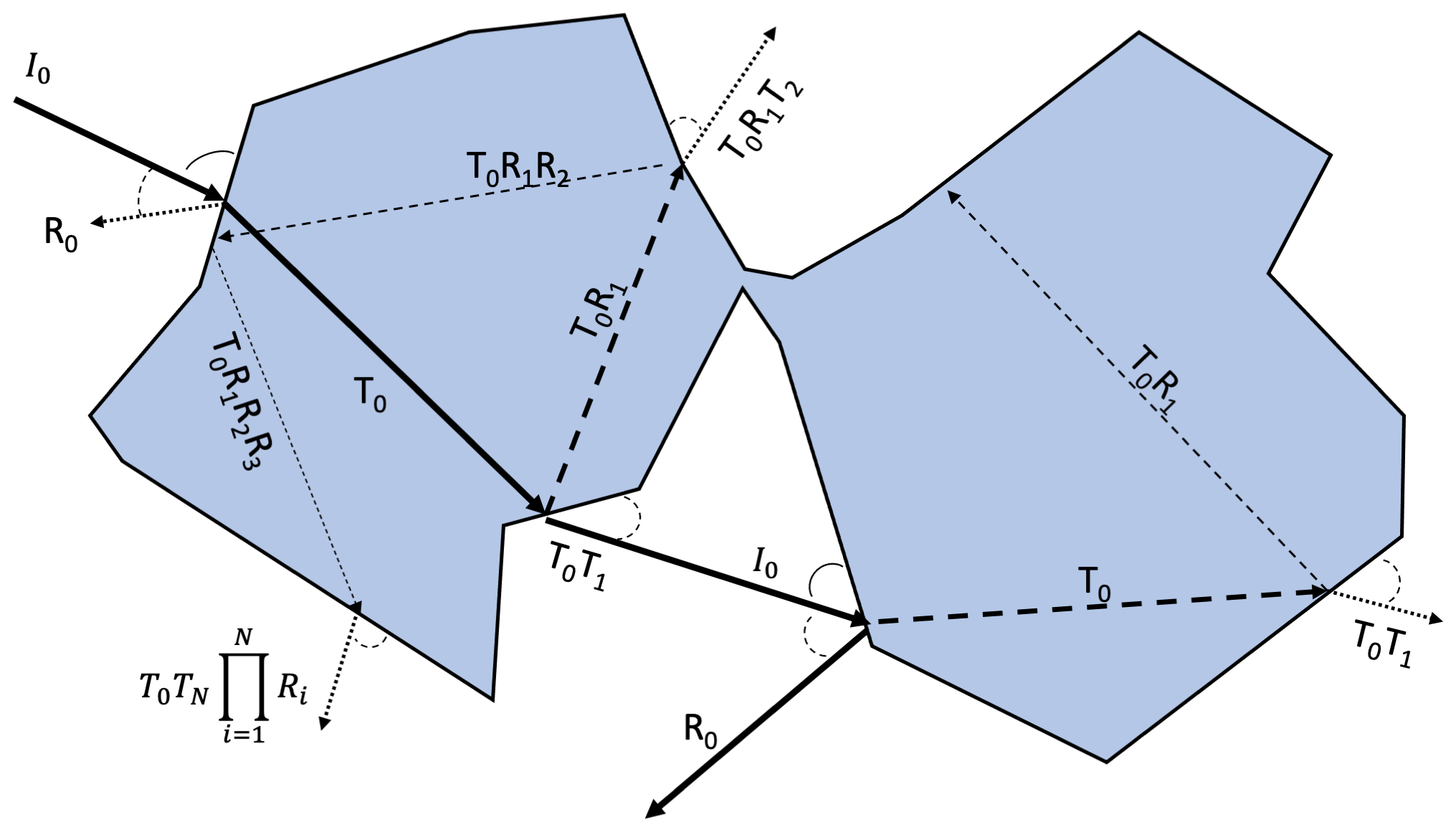
Figure 1Schematic illustrating the scattering phase function. The thick solid lines represent the actual photon track through the medium. Dashed lines within the ice phase represent the extended internal rays that are followed until 99 % of the energy incident upon the mesh surface is scattered. Scattered rays following the extended ray path are indicated by the dotted lines within the air phase and are annotated with their respective weights (W).
At the end of the ray-tracing model, the resulting distribution of energy, integrated over all photon tracks, is converted to a phase function defined relative to the total energy initially incident on the air–ice boundaries (Grundy et al., 2000):
where N is the total photon energy and Nj is the total photon energy directed into bin j. In this study, the number of bins used to represent the phase function is 180. Accordingly, dΘ=1∘. To illustrate this component of the model, the optical properties for an example snow mesh are shown in Fig. 2.
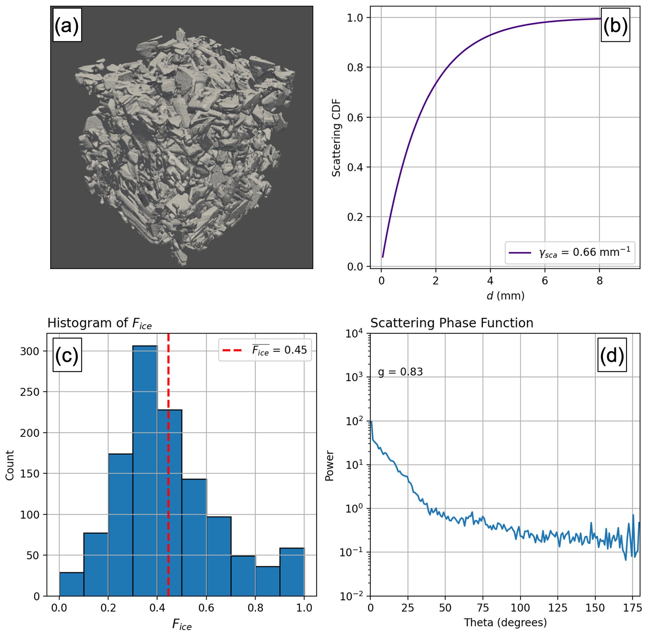
Figure 2(a) Three-dimensional rendering of the snow sample used to generate the optical properties. (b) Cumulative distribution function of scattering as a function of distance (mm) and γsca. (c) Histogram of Fice. The dashed red line indicates the mean value. (d) Scattering phase function. A total of 1200 individual photon tracks were used to generate the optical properties shown in this figure. The asymmetry parameter (g) is the average of the geometric asymmetry parameter computed from the phase function as and the diffraction asymmetry parameter gD≃1 according to Kokhanovsky and Zege (2004) and Libois et al. (2013).
2.2 One-dimensional plane-parallel photon-tracking model
Once the optical properties of the snow sample are determined by launching photons through µCT sample volumes, the plane-parallel model is used to simulate snow spectral albedo, transmittance, and the bidirectional reflectance distribution function (BRDF). The plane-parallel model is used in place of a brute-force application of the explicit photon-tracking model described by Kaempfer et al. (2007) in order to allow for the computationally feasible simulation of spectral albedo and transmittance for snow covers with depths exceeding 1 cm with sufficient grain resolution. Additionally, it is used to avoid complications associated with lateral boundary treatment and stitching multiple µCT scans together into a single coherent snow lattice.
The model used here is largely based on the framework presented in Jacques (2010) and is similar to the model described in Picard et al. (2016), which track individual photon packets as they follow unique paths through the specified media. Here, discrete snow layers with optical properties constant throughout each layer are first prescribed. Then initial photon vector positions (X0) with cartesian components of (x0, y0, z0) are specified with random x and y coordinates and z coordinates equal to the snow surface height. Each photon packet is given an initial energy of unity (E=1) and an initial direction vector (V0):
where θ is the solar zenith angle and ϕ is the azimuth angle clockwise from x. The initial direction can be prescribed as downward pointing with uniformly random zenith and azimuth angles representing isotropic diffuse radiation, as any specified zenith and azimuth angle (i.e., direct radiation), or as a mixture of both diffuse and direct radiation.
For a given photon, once the position is set, the photon is launched into the medium and travels a distance s before experiencing a scattering event. s is computed statistically using the Beer–Lambert law and the medium scattering coefficient (Jacques, 2010):
where ζ is a random uniform number between 0 and 1. The new position in the medium is
At the scattering event, the photon packet is given a new direction unit vector according to the scattering phase function. Because this framework treats the scattering phase function as a probability distribution function (PDF), the scattering angle Θ is determined by choosing a random sample from the p(cos Θ) PDF:
where P is the probability of light being scattered into a cone with solid angle dΩ in the direction Θ from the incident radiation given the phase function.
Then the new direction vector is determined from Θ (Jacques, 2010):
where ϕ is given as a uniform random number between 0 and 2π; the 0 subscript represents the incident direction; and μx, μy, and μz make up the components of the unit direction vector.
Photon energy is depleted over distance s according to the ice absorption coefficient and Fice as determined from the µCT data instead of using a medium absorption coefficient:
Here E is the new photon energy, E0 is the incident photon energy, and κλ is the wavelength-dependent absorption coefficient of ice based on the imaginary part of the refractive index k:
The parameter η is a non-dimensional scaling parameter that relates Fice, B, and ρs to absorption following expressions given in Libois et al. (2013, 2019):
where ρs is density of the snow sample. η is typically within 10 % of unity for a majority of snow samples but can enhance absorption by more than 25 % in snow with ρs>350 kg m−3 and B>1.7.
To achieve statistical energy conservation, a “Russian roulette” function is used to determine whether or not to fully absorb (i.e., kill) the photon packet once its energy falls below a prescribed threshold (Iwabuchi, 2006; Jacques, 2010). This is given as
where ζ is a random number between 0 and 1 and m is a prescribed constant on the order of 1–10. In essence, the Russian roulette technique achieves energy conservation by proportionally compensating for the energy removed from the model when photons are killed. By treating absorption continuously rather than probabilistically, the number of photons required to attain a robust solution is significantly reduced and further ensures reliable model integration.
If the z position of a photon packet with an upward trajectory is above the top of the snow surface (i.e., it has exited the top of the snowpack), the remaining energy within the packet is added to the total reflected energy and the photon is eliminated. In an open lower-boundary configuration, if a photon packet z position is less than 0 (i.e., it has exited the bottom of the snowpack), the remaining energy is added to the total transmitted energy, and the photon is eliminated. Alternatively, a lower boundary can be simulated with a specified spectral reflectance such that a portion of the photon energy will be absorbed at the lower boundary, and the remaining energy will be reflected upward. Once all photons have been eliminated from the model, the simulation is complete.
This model is extended to a multi-layer configuration by simply defining unique optical properties corresponding to specified depths throughout the snowpack. When a photon packet travels from one layer to another, its trajectory and energy depletion are determined by the optical properties of the new layer. To illustrate this, two photon tracks are plotted on a 2D plane as they travel throughout an idealized two-layer 20 cm deep snowpack (Fig. 3).

Figure 3 cross section of two photons within a multi-layered snowpack 20 cm deep. The color scale indicates the fractional energy of the photon packet. The background shading indicates the layers of the snowpack.
2.3 Directional conic reflectance function
The reflectance of a surface is often described using the concept of a BRDF (e.g., Stamnes and Stamnes, 2016). The BRDF represents the directional PDF of reflectance for a ray of light impacting the surface from a specified incident direction. To estimate the BRDF from this model, we follow the method described in Kaempfer et al. (2007), which approximates the BRDF using the directional conic reflectance function (DCRF). The DCRF is a discretized BRDF that computes the energy reflected into a cone in the direction θr, ϕr subtended by solid angle dΩ:
where I is the radiative flux and the subscripts “i” and “r” correspond to the incident and reflected radiation, respectively.
2.4 Snow sampling and spectroradiometer measurements in the field
To evaluate the model, we collected snow samples and spectral reflectance measurements of the snow surface at Union Village Dam (UVD) in Thetford, Vermont, several times throughout the 2020–2021 winter. The UVD site is a broad flat clearing surrounded by deciduous forests spanning approximately 40 000 m2 and bounded on the southern end by the Ompompanoosuc River. During each data collection, a snow pit was excavated and standard snow characteristics, such as snow depth, density, and grain size, were measured manually. Several snow samples were carefully extracted at several depths spanning the height of the snow cover in columns adjacent to the snow pit sidewalls in cylindrical containers 7 cm high × 1.9 cm in diameter, with a 1–2 cm overlap in the depth of each sample. Three replicate samples, spaced laterally <10 cm from one another, at each depth were collected. The specific samples used in this analysis were taken from the surface, 0–7 cm, in the case of the fine-grain sample and from 14–19 cm depth in the case of the coarse-grain sample. These samples were transported in a hard, plastic cooler for 10 miles (16 km) from the UVD site to the Cold Regions Research and Engineering Laboratory (CRREL). The fine-grain sample was imaged 18 d after snow sampling, while the coarse-grain sample was imaged 53 d after snow sampling. All samples were stored at −30 ∘C to limit metamorphic change in the intervening timeframe. These samples were not cast (i.e., not preserved using a pore filler).
Spectral reflectance data were collected using a Malvern Panalytical ASD FieldSpec 4 Hi-Res high-resolution spectroradiometer. The FieldSpec 4 has a spectral range of 350–2500 nm and a spectral resolution of 3 nm in the visible and 10 nm in the shortwave infrared. The data collection was performed within 1.5 h of solar noon (EST) in order to limit high-zenith-angle impacts. The FieldSpec 4 requires optimization, which adjusts and improves the detector sensitivities for the probe and light source currently in use. Optimization was conducted prior to the start of data collection and any time lighting conditions changed in order to ensure accurate reflectance readings. Data collections were taken 2.5 to 3 feet (0.75–1 m) above the snow surface at nadir using a 5∘ field-of-view optic lens, resulting in a measurement footprint diameter of approximately 6 cm. The collection strategy employed included taking a white reference reading from a pure reflective panel and five readings at different locations on the target surface; the mean of the five readings was used as the reflectance value for that specific location.
In this paper, we focus specifically on data collected on 12 February 2021 as this day had the most stable ambient lighting conditions and resulted in the majority of our snow and reflectance measurements. At the time of the measurements, the sky was covered with a high, optically thick overcast, and as a result the ambient lighting conditions were generally diffuse. The snow was dry and approximately 34 cm deep and was roughly characterized as a layer of relatively fresh snow approximately 10 cm deep overlying a layer comprised of larger mixed refrozen snow grain clusters and facets, separated by a 1 cm thick ice crust. We performed an initial evaluation of the model against measurements to focus on the effect of shallow snow on the spectral albedo.
To measure the effects of a shallow snowpack, a (40 cm × 40 cm) aluminum panel painted black was inserted horizontally into the snowpack through the snow pit sidewall at three depths (10, 4.5, and 2.5 cm) with care so as not to damage the smooth snow surface (Fig. 4). This panel was strongly absorptive in the visible and NIR spectrum with a constant reflectance of approximately 4 % throughout the entire 350–2500 nm range. Since there was no appreciable difference between the measured spectral albedo of the virgin snow (i.e., no inserted panel) and the panel inserted at 10 cm, we limit our analysis to the 4.5 and 2.5 cm panel depths.
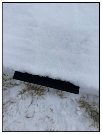
Figure 4Photograph of the black aluminum panel inserted into the snow pit sidewall approximately 2.5 cm from the surface.
2.5 µCT sampling and mesh generation
The snow samples were characterized at the microscale with a cold-hardened Bruker SkyScan 1173 µCT scanner housed in a −10 ∘C cold room equipped with a Hamamatsu 130/300 tungsten X-ray source, which produces a fixed conical, polychromatic beam with a spot size of <5 µm and a flat panel sensor camera detector. Each sample was scanned with 38 kV X-rays at 196 mA and a nominal resolution of approximately 20 µm as the sample was rotated 180∘ in 0.6∘ steps with an exposure time of 300–350 ms. Based on estimates of the minimum grain size from manual field measurements, the resolution of the µCT, at 20 µm, is roughly on the order of the linear size of the minimum grain size we were imaging. We used the commonly employed Nyquist sampling criterion, which requires a minimum of 2.3 pixels per linear feature, to determine that the resolution was sufficient for the grain sizes we sampled. X-rays were detected using a 5 MP (2240×2240) flat panel sensor utilizing 2×2 binning, and projection radiographs were averaged over four frames. The resulting 1120×1120 px radiographs were then reconstructed into 2D grayscale horizontal slices using NRecon software (Bruker), which utilizes a modified Feldkamp cone-beam algorithm to produce a vertical stack of grayscale cross-section images. Image reconstruction processing included sample-specific post alignment, Gaussian smoothing using a kernel size of 2 to reduce noise, sample-specific ring artifact correction of dead pixels, beam hardening correction, and X-ray source thermal drift correction. A cylindrical volume of interest with a diameter of 1.6 cm was selected from the scanned samples in order to eliminate edge effects caused by the sampling process.
Resulting grayscale images are segmented into two phases: air (lowest X-ray absorption) and snow (highest X-ray absorption). Segmenting thresholds for each phase are determined by finding the local minimum between peaks on the histogram showing all grayscale values and using that value as a global threshold for each scanned sample. The resulting binarized data are despeckled so that any objects less than 2 pixels in diameter were removed.
The final binarized images are then used to construct 3D representations of dry-snow samples for input into the RTM. This is accomplished through the use of open-source image processing and 3D visualization software packages accessed through Python (Schroeder et al., 1996; Van der Walt et al., 2014; Sullivan and Kaszynski, 2019).
To build a full sample mesh, a contour-based surface reconstruction process was developed to generate snow surfaces from the voxels that make up the snow sample. This method uses a subset of the binary sample array, including both snow and adjacent air voxels. The subset array is then refined to increase the resolution. A Gaussian filter is applied to smooth the refined array, diminishing the pixelated appearance of the voxelized snow–air interface and producing a smooth level set from which to extract the snow surface. The smoothed level set is then used to define an isosurface at the snow–air boundary, providing control over where the boundary is drawn with respect to the voxels.
Finally, to extract the isosurface from the 3D voxel array, we apply the marching cubes method. This algorithm iterates through defined cubes (i.e., voxels) and determines, through knowledge of the pixel values at the cube vertices, if the isosurface intersects that cube. If so, it creates triangular patches via a lookup table that are eventually connected to form the isosurface boundary. The original algorithm presented by Lorensen and Cline (1987) can lead to cracks and over the years has been improved by many (Nielson and Hamann, 1991; Scopigno, 1994; Natarajan, 1994; Chernyaev, 1995; Lewiner et al., 2003). For this work, we used the adaptation implemented by Lewiner et al. (2003), which improved the algorithm to resolve face and internal ambiguities, extended the lookup table, and guaranteed correct topology. As a final step, each grain is “repaired” to remove any defects and degenerate elements and ensure a manifold surface according to Attene (2010) and then decimated to reduce the overall number of triangles that comprise the surface, thereby lowering the computational requirements. Overall, this method appears to accurately characterize the snow within the µCT sample with computed mesh snow sample densities within 1.5 % of snow densities computed from the raw voxels. Figure 5 shows a 2D cross section comparing air–ice boundaries to the raw pixels of the image, and selected example 3D-rendered µCT samples are shown in Fig. 6.
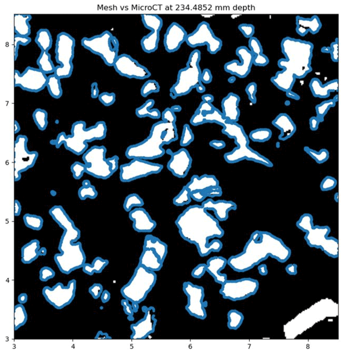
Figure 5A 2D cross-sectional slice of a binarized µCT scan with corresponding mesh boundaries superimposed shown as the blue lines.
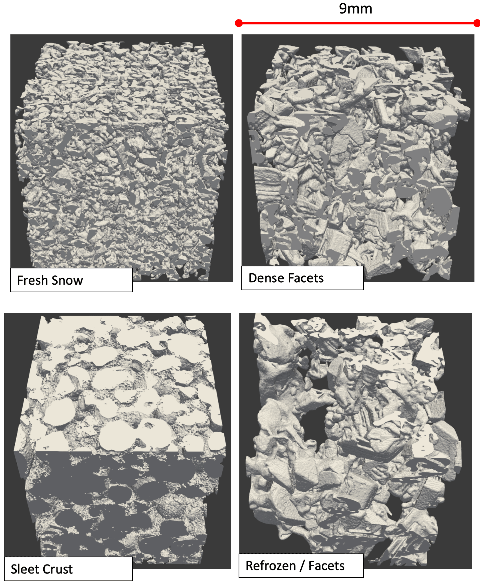
Figure 6Example 3D renderings of selected µCT samples representing different types of snow grain.
3.1 General evaluation
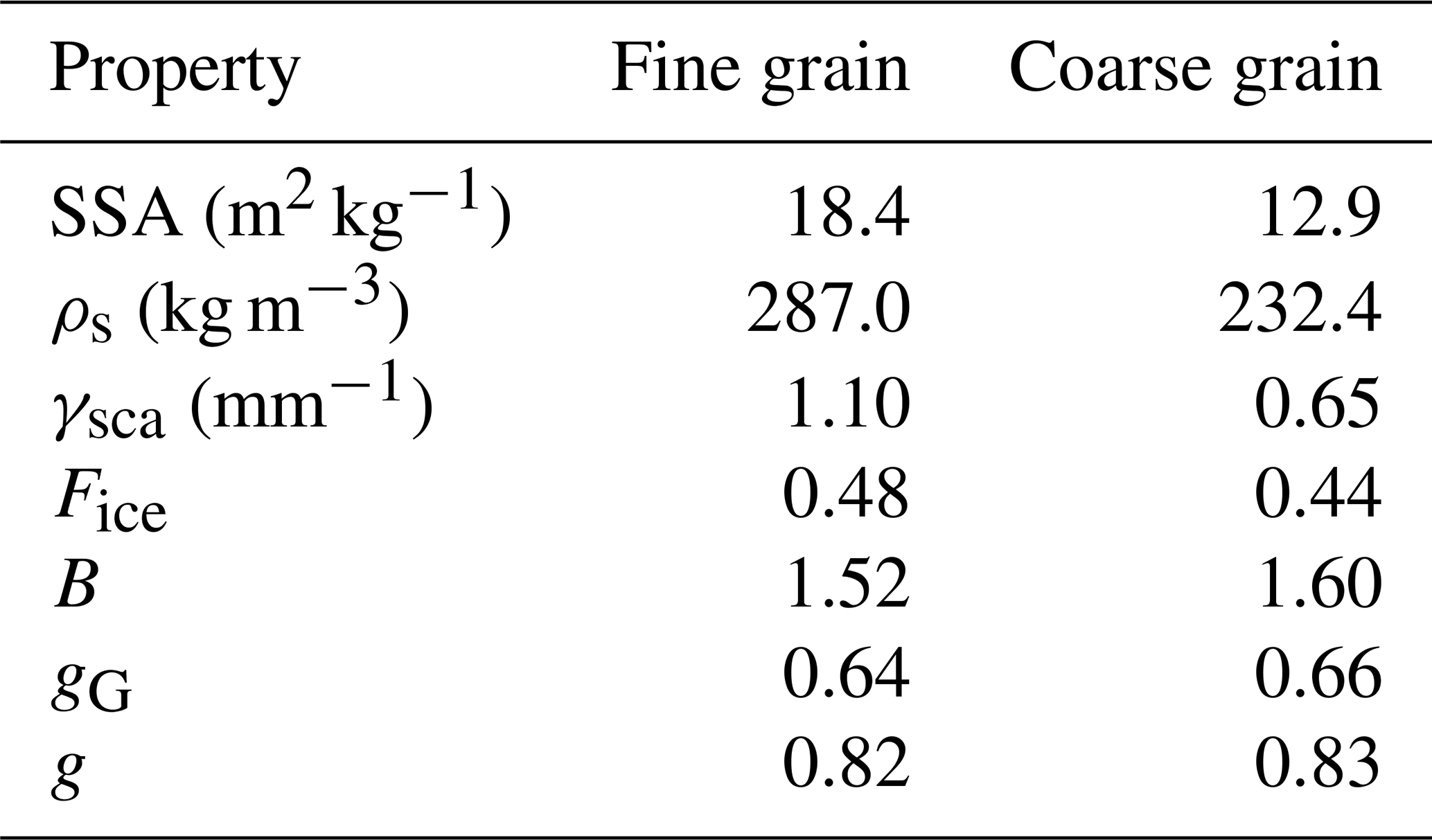
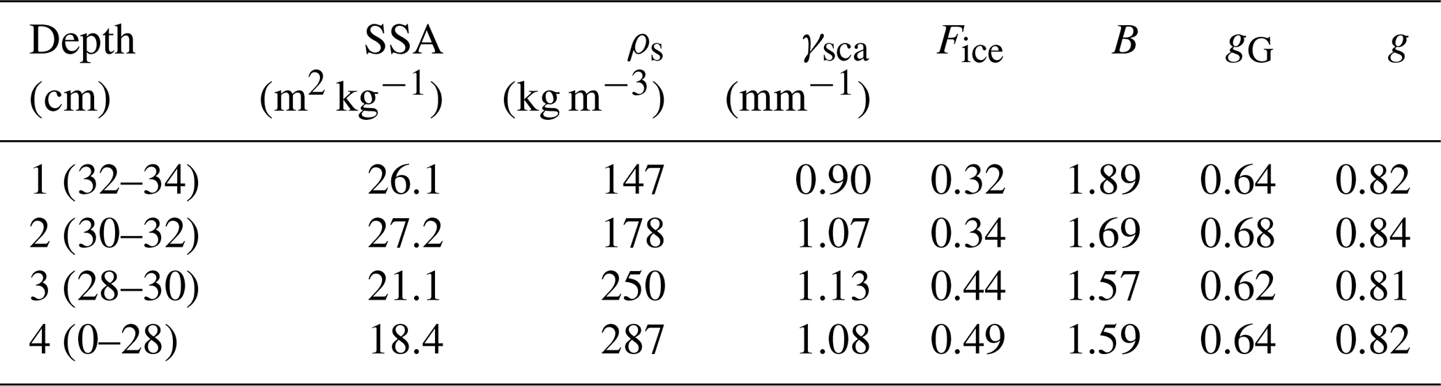
An initial evaluation of the model is performed by simulating the spectral albedo for two idealized 60 cm deep snowpacks with uniform optical properties throughout. For these snowpacks, the optical properties are determined from 3D meshes generated by two characteristically distinct µCT samples. One mesh is representative of fresh, fine-grained snow near the surface and the other of large facets near the bottom of the snowpack (Fig. 7). For each mesh, the total mesh volume is approximately 800 mm3. Additional physical and optical properties of each mesh are presented in Table 1. For each sample, the spectral albedo is computed for wavelengths between 400–1600 nm at 20 nm intervals with diffuse incident radiation. This comparison demonstrates that the model capably reproduces a known behavior of spectral albedo, namely the strong sensitivity of NIR albedo to snow microstructure (Fig. 8). The spectral albedo is relatively uniform between the two snowpacks for the spectral range between 400 and 800 nm, and then the albedos diverge, with a more rapid decrease in albedo for the coarse-grain snow.

Figure 7Three-dimensional renderings of mesh samples used to generate the optical properties for the general evaluation and snow transmittance comparisons. (a) Fine-grain sample and (b) coarse-grain sample.
Table 1Physical and optical properties of the fine-grain and coarse-grain mesh samples. Note that SSA (snow specific surface area) and ρs are computed directly from the µCT sample. The geometric (gG) and total asymmetry parameters (g) are computed as described in Fig. 2.
We then assess the dependence of simulated spectral albedo on incident zenith angle for the fine-grain snow sample at four different wavelengths to evaluate the model's ability to simulate anisotropy in the surface reflectance (Fig. 9). This analysis shows an increase in albedo at high zenith angles that is most pronounced in the NIR, which represents the functional dependence between albedo and cos (θ). This result is broadly consistent with results from previous studies that compare snow albedo and the zenith angle (e.g., Li and Zhou, 2003; Kokhanovsky and Zege, 2004; Xiong et al., 2015). As a related evaluation, the model-simulated DCRF is computed as a function of the zenith angle (Fig. 10). This analysis reveals that the reflectance is mostly isotropic for zenith angles less than approximately 55∘, at which point the surface becomes increasingly forward scattering, consistent with previous observational and modeling studies (Aoki et al., 2000; Hudson et al., 2006; Kaempfer et al., 2007; Dumont et al., 2010; Xiong et al., 2015; Jiao et al., 2019).
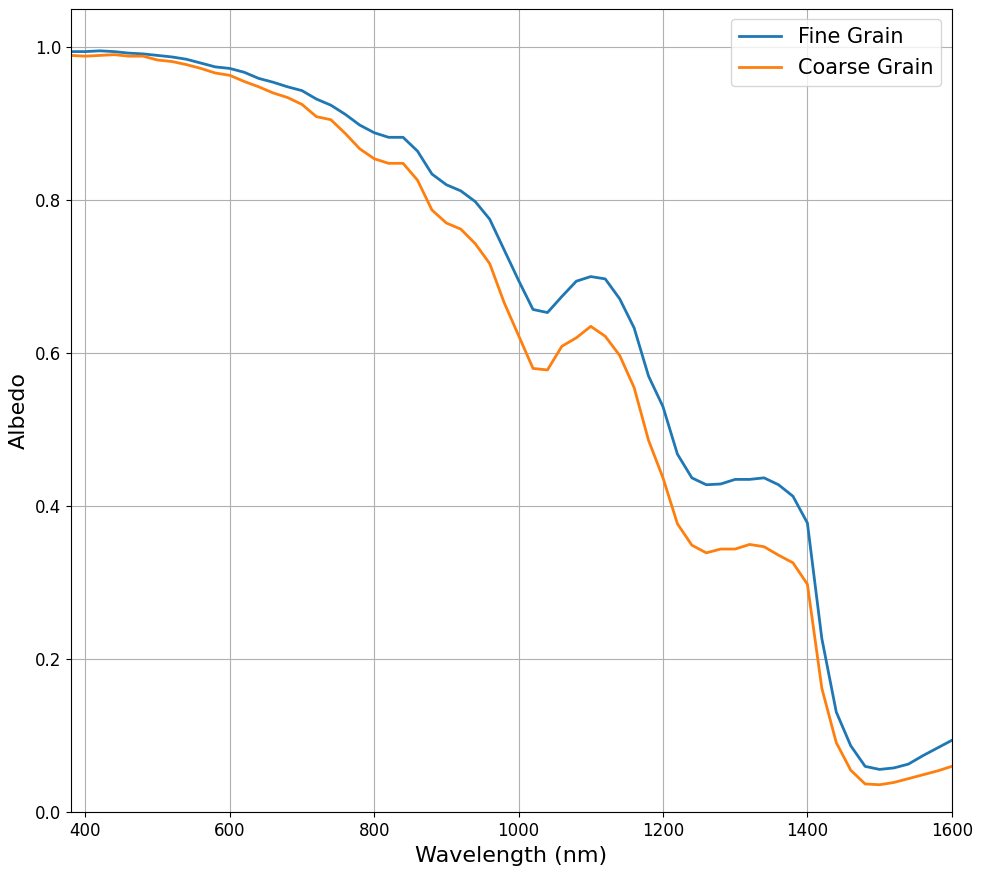
Figure 8Simulated spectral albedo for fine-grain and coarse-grain snow samples for 100 % diffuse radiation. Note these simulations were run with 25 000 photons for a snow depth of 60 cm.
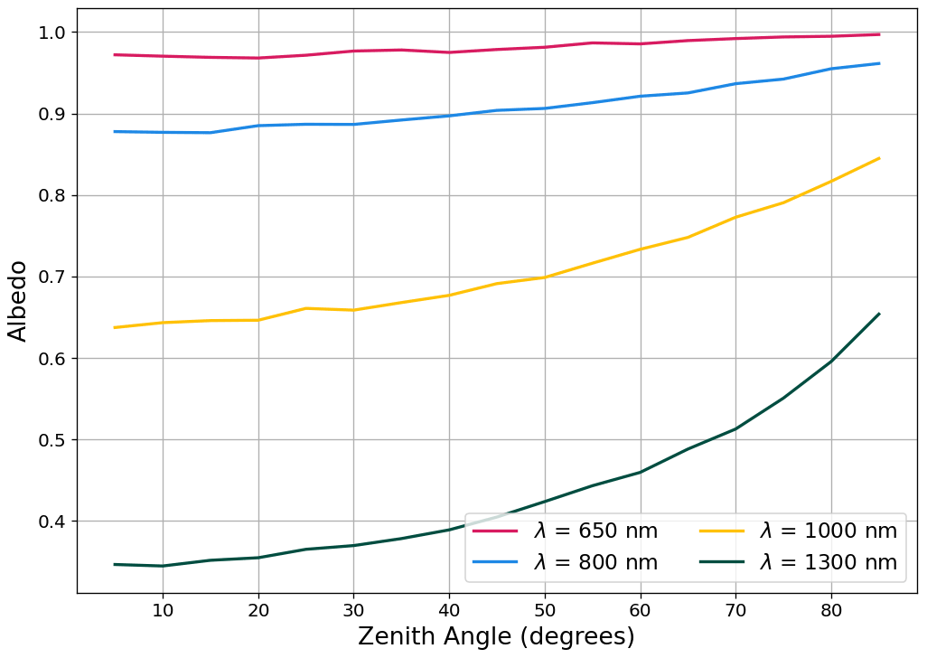
Figure 9Simulated spectral albedo as a function of the incident zenith angle for selected wavelengths. Note these simulations were run with 25 000 photons for a snow depth of 60 cm.

Figure 10Polar plots of DCRF at 1000 nm for incident zenith angles ranging from 5–85∘. The reflected azimuthal direction is on the theta axis, and the reflected zenith angle is on the r axis. Color scale ranges from 0–1.5.
Finally, we use the model to provide an initial assessment of the impacts of snow microstructure on simulated spectral transmittance at specified depths within a homogenous snowpack. To accomplish this, the optical properties of the µCT samples in Fig. 7 are used to simulate and compare the spectral transmittance at varying depths (Fig. 11). The transmittance is highest at the short, non-absorptive wavelengths and gradually decreases throughout the NIR, broadly matching quantitative snow transmittance results reported in Perovich (2007) and Libois et al. (2013). The depth of the 5 % transmittance contour for the fine-grain snow sample is approximately 6 cm for the visible and decreases to approximately 2 cm for the NIR (Fig. 11a), indicating that the fine-grain snow penetration length is on the order of only a few centimeters. In contrast, the transmittance for the coarse-grain snow is greater near the surface, and the depth of the 5 % contour correspondingly increases to 12.5 cm for the visible and 5 cm for the NIR (Fig. 9b).
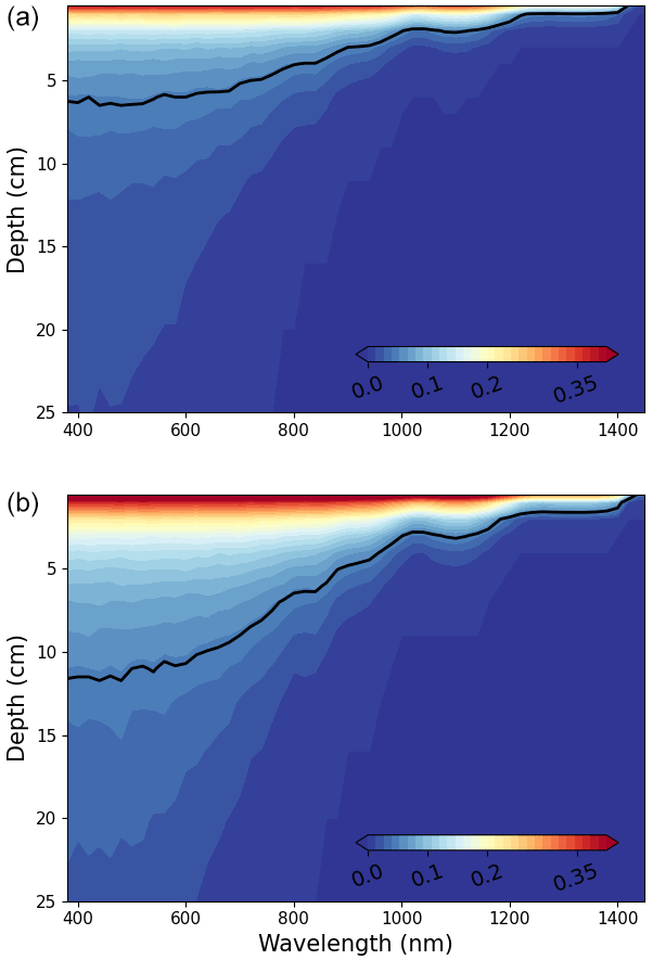
Figure 11Simulated transmittance of (a) the fine-grain snow and (b) the coarse-grain samples contoured as a function of depth and wavelength. Solid black lines mark the depth of the 5 % transmittance contour.
3.2 Evaluation against UVD data
To evaluate the model's ability to simulate the effect of the underlying surface on snow spectral albedo for shallow snow, optical properties used in the plane-parallel model were determined from four approximately 800 mm3 µCT samples, with each sample representing a 2 cm thick layer within the top 8 cm of the snowpack. The RTM is then configured with four layers according to these optical properties (given in Table 2). The top three layers are each 2 cm thick, and the bottom layer is 28 cm thick, such that the entire snow depth amounts to 34 cm. We chose this configuration in accordance with the hypothesis that the snow microstructure below 8 cm had little impact on the measured surface spectral albedo. To simulate the panels, the snowpack depth is modified to be 4.5 and 2.5 cm deep with a lower boundary consistent with the spectral reflectively of the black panel (Table 2).
Table 2Physical and simulated optical properties of the top 8 cm of snow measured at the UVD site on 12 February 2021. SSA and ρs are computed directly from the µCT sample. Note that the depths correspond to the RTM depths for the virgin snow calculation. The geometric (gG) and total asymmetry parameters (g) are computed as described in Fig. 2.
There is generally good agreement between the observations and the model (Fig. 12), and in particular, the model accurately simulates the impact of the inserted panel on the surface albedo for wavelengths shorter than 1000 nm for both the 4.5 and the 2.5 cm depths. The model spectral albedo decreases more rapidly than the observations with wavelengths in the 800–1000 nm region, particularly for the virgin snow sample. This leads to a slight underestimate in albedo in the NIR range for wavelengths shorter than 1400 nm. We suspect that beyond 1400 nm, differences between the model and observations are due to the limitations of the assumptions made as part of the geometric optics approximation as the approximate particle size parameter is <1000 for λ>1400 nm. The simulated spectral albedos converge to the same value at approximately 950 nm, which matches the observed behavior of measurements collected over 4.5 and 2.5 cm panel depths. This behavior does not match the observed behavior of the virgin snow, which has an albedo higher than the panel observations until approximately 1400 nm. It is unknown if the cause of this difference is due to the model or is related to observational uncertainty caused by imperfect lighting conditions. Therefore, we are careful to note that this comparison is presented as an initial evaluation of our modeling framework and not a robust evaluation of its accuracy.
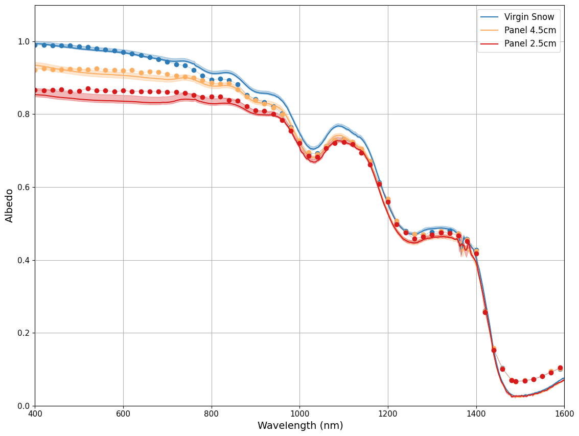
Figure 12Simulated and observed spectral albedo for three different snow depths. The solid lines indicate observations, and dotted lines indicate simulations. The shading around the observations indicates the inter-quartile range of the measurements computed from the five snow and two reference scans collected during each measurement, providing an assessment of measurement uncertainty. The mean RMSE of the simulated albedo compared to measurement-derived albedo over 400–1600 nm is equal to 0.03.

Figure 13Optical properties for λ=1000 nm computed from µCT photon tracking compared against sample physical properties. (a) Fice vs. ρs and (b) γsca vs. SSA ⋅ρs. Linear regression lines are shown in dashed black lines. Marker shapes and colors are indicative of the observed grain forms determined through visual assessment during snow pit analysis. Note that in panel (b) a histogram of the estimated B parameters for all of the µCT samples is shown, inset. Bmean=1.53 is shown as the vertical red line.
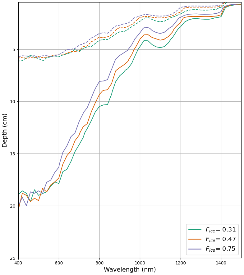
Figure 14Depth of simulated 5 % transmittance contour as a function of the wavelength for varying Fice at two scattering coefficients: γsca=0.39 (solid lines) and γsca=1.29 (dashed lines).
3.3 Snow optical and physical properties
The first component of the model is used independently of the plane-parallel model to assess the relationship between common snow physical properties and the simulated optical properties from this framework. To demonstrate this, we compare snow specific surface area (SSA) and snow sample density (ρs) to γsca and Fice. This analysis is performed by generating optical properties from several µCT sample volumes collected on different dates and locations during the 2020–2021 winter season, spanning a wide range of snow types. Note that each µCT sample is approximately 800 mm3 and the sample SSA and ρs are determined from the µCT 3D rendering.
This analysis reveals that Fice has a very robust relationship with snow density (Fig. 13a) described by the following linear fit:
with R2=0.92. In Fig. 13b, γsca is compared to the product of ρs and SSA, to match the analytical formula described in Kokhanovsky and Zege (2004). The results show a clear linear relationship fit to
with R2=0.78.
The estimated B parameter is distributed normally around a mean of 1.49, consistent with the results reported in Libois et al. (2014). We note that there is no significant relationship between B and snow grain form or size; however there is a general tendency for B to be highest for samples with higher SSA and smaller grains, which is qualitatively consistent with Kokhanovsky and Zege (2004) and Libois et al. (2014).
To further assess how these two specific snow optical properties, γsca and Fice, affect the greater simulated spectral transmittance, we perform a sensitivity analysis by comparing the 5 % transmittance contour depth for three fractional ice paths – 0.31, 0.47, and 0.75 – at two fixed γsca values: 1.29 and 0.39 mm−1 (Fig. 14). The two γsca values correspond to the max and min values found in the previous analysis and presented in Fig. 13b. The three Fice values correspond to the max, min, and mean values (Fig. 13a). We compare the influence of Fice at both the max and min γsca values, since we anticipate the strength of its influence will vary according to γsca. We note that high values of γsca are more likely to coincide with high values of Fice due to the shared dependence of these variables on snow density in most snowpacks.
The results of this analysis indicate that both γsca and Fice impact snow transmittance in accordance with relationships discussed in Libois et al. (2013). Specifically, the approximate factor-of-3 decrease in the scattering coefficient corresponds to an approximate factor-of-3 increase in depth of the 5 % transmittance contour, consistent with a linear relationship between γsca and penetration depth (L). Additionally, the simulated factor increase in penetration depth is approximately the square root of the factor increase in Fice, for λ>600 nm, consistent with the presented in Libois et al. (2013).
Overall, this framework shows promise as a research tool for better understanding visible and NIR snow radiative transfer through snowpacks with irregularly shaped and arranged grains. However, there are numerous uncertainties in this framework that should be addressed in future work to better understand its capabilities and limitations.

Figure 15Snow pit stratigraphy (left) compared against γsca, Fice, ρs, and SSA. Each dot represents a µCT sample at a specified depth. Violin plots show estimated probability distributions for each observer-identified snow layer according to the samples collected with the layer.
For instance, there are broader questions surrounding the definition of the scattering coefficient γsca and the phase function p(cos Θj) for weakly absorbing porous media in the geometric optics limit. While, fundamentally, γsca is the inverse of the mean free path traveled by a photon between scattering events within the medium, there is some ambiguity as to how a scattering event is defined. Traditionally and in most applications, a scattering event is defined as occurring at a particle. That is, light intersects a particle and is scattered away from the particle, and internal reflections within the particle are considered part of a single, larger scattering event (e.g., Van De Hülst, 1957; Kokhanovsky and Zege, 2004; Randrianalisoa and Baillis, 2010; Malinka, 2014). However, more recent studies have considered scattering along dielectric boundaries separating the air–ice phase such that internal reflections within a given particle are counted as distinct scattering events (e.g., Xiong et al., 2015). While ray-tracing techniques such as the one presented here are well suited to the latter definition, this model conforms to the former, “particle”, approach such that the optical properties generated are consistent with a majority of accepted methods. However, we note that reconciling these definitions is a worthy topic of future research and that the model framework presented here is a potentially useful tool for these efforts.
An additional source of uncertainty in computing the optical properties is the method used to estimate the absorption enhancement parameter B directly from ray tracing. Formulas presented in Libois et al. (2019) show that B can be related to Fice and snow density following
However, estimating B from the sample density and Fice generally leads to values much larger than those computed from Eq. (8). We speculate that this discrepancy is due to the fact that some photon tracks through the rendered mesh do not adequately represent the snow sample. Specifically, some photons traveling through the mesh take short paths through a single particle before exiting the sample, resulting in an Fice close to 1. This is supported by the presence of a peak at 0.95 in the histogram of Fice shown in Fig. 2b. Since Eq. (24) indicates a non-linear increase in B with Fice, these non-representative paths have a disproportionately large influence on B in Eq. (24).
Another possible source of uncertainty in this framework is the assumption that the optical properties computed from volume µCT samples on the order of 1 cm3 are homogeneous laterally and can be extrapolated to characterize representative layer depths. To elucidate upon this uncertainty, we compare the optical and physical properties of the 20 rendered µCT samples collected at UVD on 12 February 2021 to the observed snow pit stratigraphy (Fig. 15). Here we show that the top layer of the snowpack has more homogeneous physical and optical properties than the buried layers. In particular there is substantial variability in γsca and Fice within the rounded grains and the uppermost facet layers. Further investigation into this variability in the facet layer spanning the 14–18 cm layer reveals that this variability is caused largely by the fact that some µCT samples within this layer contained unusually large pore spaces, which caused lower SSA and γsca values. We suspect that this variability has limited impacts on the simulated spectral albedo for the shallow snow simulations, since the top snow layer is relatively homogeneous. However, this variability is likely to have more significant impacts for simulations focused on older snowpacks with larger and less uniformly distributed snow grains.
Finally, there are several assumptions we used to simplify our model that are worth additional discussion. First, we have taken the real part of the ice refractive index to be constant at 1.30, which is the refractive index of ice at λ=1000 nm. While this is generally a good assumption, there is a minor wavelength dependence throughout the visible and NIR range that could affect the optical properties of the medium and potentially influence the plane-parallel model. Further, it has been shown that spectral albedo in the NIR (λ>1400 nm) is sensitive to which refractive index database is used to represent absorption (Carmagnola et al., 2013; Dumont et al., 2021). While we do not explore this sensitivity here, we note it as a potential source of error. Finally, the derivation of optical properties is based on the underlying assumption that snow is weakly absorbing such that γext can be approximated with γsca. While snow is weakly absorbing in the visible range, it is more absorptive in the NIR, and accordingly we expect that this assumption can lead to increased uncertainty beyond 1400 nm. Despite these sources of potential uncertainty, as demonstrated in Fig. 12, simulated and observed albedos are in good agreement for λ<1400 nm.
In this work we have presented a blended photon-tracking radiative transfer model in an effort to better understand the complicated influence of snowpack microstructure on snow spectral transmittance in the geometric optics limit. A primary goal of this modeling approach is to expand upon previous approaches aimed at incorporating 3D renderings of real snow microstructure into radiative transfer models for snowpacks of arbitrary depth while maintaining the ray-tracing methods utilized in the original Kaempfer et al. (2007) model. To accomplish this, existing methods for simulated photon interactions with rendered elements are employed to determine key optical properties of the snow (Grundy et al., 2000; Kaempfer et al., 2007; Randrianalisoa and Baillis, 2010).
An evaluation of this framework for consistency with known behavior of spectral snow albedo revealed that this framework can successfully reproduce the dependency of spectral albedo and grain size, as well as the surface anisotropy at high incident zenith angles, found in previous studies. Furthermore, an initial comparison of the simulated snow albedo against albedo measured in the field over snow with varying depths indicates that the model can simulate the effects of an underlying surface on spectral albedo with sufficient accuracy.
In comparing two different snow samples, it was revealed that snow microstructure has a large impact on snow transmittance in the visible spectrum and near the snow surface, increasing the 5 % transmittance depth at 400–650 nm from approximately 6 cm for a fine-grain snow sample to 12.5 cm depth for a coarse-grain sample. These values and the ability to further constrain the transmittance depths of shallow snowpacks will allow for improved capabilities for determining the optical properties of shallow snowpacks. A brief sensitivity analysis of the optical properties revealed that lowering the medium scattering coefficient acted to increase the transmittance depth in the visible bands, while the ice path fraction (Fice) impacted the rate at which albedo and transmittance decreased as a function of wavelength in the NIR.
Overall, while current efforts are focused on using this model to better understand snow transmittance, it shows promise as a broadly applicable snow RTM that has a strong direct connection to µCT snow samples. While currently it is limited to the geometric optics approximation for clean snow and unpolarized radiation, ongoing and anticipated future efforts are aimed at incorporating polarization, parameterizing diffraction, and including light-absorbing particulates (LAPs). In particular, recent multiphase image segmentation techniques (West et al., 2018; Hagenmuller et al., 2019) could be used to better separate snow, air, and LAPs in a µCT sample allowing for the impact of LAPs to be determined through ray tracing. Furthermore, because the model operates entirely as a photon-tracking model, it is a natural fit with macroscale ray tracing and therefore could be used to investigate the reflectance of rough snow surfaces such as sun cups or sastrugi.
The mesh generation and radiative transfer model code are publicly available at https://doi.org/10.5281/zenodo.7086881 (Letcher and Parno, 2022a). Supporting ASD data and analysis code are publicly available at https://doi.org/10.5281/zenodo.7083432 (Letcher and Parno, 2022b).
TL performed a majority of the model physics implementation, structural development, and coding, in addition to coordinating the model analysis and manuscript preparation. JP led research and coding efforts related to the 3D mesh generation and rendering and performed major research and coding efforts related to the first component of the model; she also coordinated a majority of the fieldwork activity. ZC provided research support, participated in snow sampling, and coordinated µCT analysis. LF performed a large portion of µCT scans and a majority of the µCT image post-processing and analysis. JO participated in fieldwork and provided background on the ASD instrumentation and sampling for the paper. TL, JP, and JO performed the RTM simulations and assisted in code debugging. All authors provided writing support for the paper.
The contact author has declared that none of the authors has any competing interests.
Publisher's note: Copernicus Publications remains neutral with regard to jurisdictional claims in published maps and institutional affiliations.
We wish to acknowledge Arnold Song from Dartmouth College in Hanover, New Hampshire, for providing relevant code examples to facilitate 3D shape rendering. We also wish to thank Taylor Hodgdon from CRREL for providing occasional support and advice on using Python to perform mesh generation and rendering. We thank Bert Davis and Ned Bair for providing valuable initial feedback on the manuscript. Finally, we would like to sincerely thank the assigned journal editor and the reviewers for providing thorough and engaging rounds of review which substantially improved the quality of this paper.
This research has been supported by the Engineer Research and Development Center (Cold Weather Military Research).
This paper was edited by Marie Dumont and reviewed by Quentin Libois and one anonymous referee.
Adolph, A. C., Albert, M. R., Lazarcik, J., Dibb, J. E., Amante, J. M., and Price, A.: Dominance of grain size impacts on seasonal snow albedo at open sites in New Hampshire, J. Geophys. Res.-Atmos., 122, 121–139, 2017. a
Aoki, T., Aoki, T., Fukabori, M., Hachikubo, A., Tachibana, Y., and Nishio, F.: Effects of snow physical parameters on spectral albedo and bidirectional reflectance of snow surface, J. Geophys. Res.-Atmos., 105, 10219–10236, 2000. a, b, c
Attene, M.: A lightweight approach to repairing digitized polygon meshes, The visual computer, 26, 1393–1406, 2010. a
Bair, E. H., Rittger, K., Skiles, S. M., and Dozier, J.: An examination of snow albedo estimates from MODIS and their impact on snow water equivalent reconstruction, Water Resour. Res., 55, 7826–7842, 2019. a
Bohren, C. F. and Beschta, R. L.: Snowpack albedo and snow density, Cold Reg. Sci. Technol., 1, 47–50, 1979. a
Carmagnola, C. M., Domine, F., Dumont, M., Wright, P., Strellis, B., Bergin, M., Dibb, J., Picard, G., Libois, Q., Arnaud, L., and Morin, S.: Snow spectral albedo at Summit, Greenland: measurements and numerical simulations based on physical and chemical properties of the snowpack, The Cryosphere, 7, 1139–1160, https://doi.org/10.5194/tc-7-1139-2013, 2013. a
Chernyaev, E.: Marching cubes 33: Construction of topologically correct isosurfaces, Tech. rep., in: CERN Report, CN/95-17, http://wwwinfo.cern.ch/asdoc/psdir (last access: February 2022), 1995. a
Dang, C., Fu, Q., and Warren, S. G.: Effect of snow grain shape on snow albedo, J. Atmos. Sci., 73, 3573–3583, 2016. a
Déry, S. J. and Brown, R. D.: Recent Northern Hemisphere snow cover extent trends and implications for the snow-albedo feedback, Geophys. Res. Lett., 34, L22504, https://doi.org/10.1029/2007GL031474, 2007. a
Dickinson, R. E.: Biosphere atmosphere transfer scheme (BATS) version 1e as coupled to the NCAR community climate model, NCAR Tech. Note TH-387+ STR, 1993. a
Doherty, S. J., Warren, S. G., Grenfell, T. C., Clarke, A. D., and Brandt, R. E.: Light-absorbing impurities in Arctic snow, Atmos. Chem. Phys., 10, 11647–11680, https://doi.org/10.5194/acp-10-11647-2010, 2010. a
Dumont, M., Brissaud, O., Picard, G., Schmitt, B., Gallet, J.-C., and Arnaud, Y.: High-accuracy measurements of snow Bidirectional Reflectance Distribution Function at visible and NIR wavelengths – comparison with modelling results, Atmos. Chem. Phys., 10, 2507–2520, https://doi.org/10.5194/acp-10-2507-2010, 2010. a
Dumont, M., Brun, E., Picard, G., Michou, M., Libois, Q., Petit, J., Geyer, M., Morin, S., and Josse, B.: Contribution of light-absorbing impurities in snow to Greenland’s darkening since 2009, Nat. Geosci., 7, 509–512, 2014. a
Dumont, M., Flin, F., Malinka, A., Brissaud, O., Hagenmuller, P., Lapalus, P., Lesaffre, B., Dufour, A., Calonne, N., Rolland du Roscoat, S., and Ando, E.: Experimental and model-based investigation of the links between snow bidirectional reflectance and snow microstructure, The Cryosphere, 15, 3921–3948, https://doi.org/10.5194/tc-15-3921-2021, 2021. a, b
Flanner, M. G. and Zender, C. S.: Linking snowpack microphysics and albedo evolution, J. Geophys. Res.-Atmos., 111, D12208, https://doi.org/10.1029/2005JD006834, 2006. a
Flanner, M. G., Shell, K. M., Barlage, M., Perovich, D. K., and Tschudi, M.: Radiative forcing and albedo feedback from the Northern Hemisphere cryosphere between 1979 and 2008, Nat. Geosci., 4, 151–155, 2011. a
Gardner, A. S. and Sharp, M. J.: A review of snow and ice albedo and the development of a new physically based broadband albedo parameterization, J. Geophys. Res.-Earth Surf., 115, F01009, https://doi.org/10.1029/2009JF001444, 2010. a
Grenfell, T. C. and Perovich, D. K.: Radiation absorption coefficients of polycrystalline ice from 400–1400 nm, J. Geophys. Res.-Oceans, 86, 7447–7450, 1981. a
Grundy, W., Douté, S., and Schmitt, B.: A Monte Carlo ray-tracing model for scattering and polarization by large particles with complex shapes, J. Geophys. Res.-Planets, 105, 29291–29314, 2000. a, b, c, d
Hagenmuller, P., Flin, F., Dumont, M., Tuzet, F., Peinke, I., Lapalus, P., Dufour, A., Roulle, J., Pézard, L., Voisin, D., Ando, E., Rolland du Roscoat, S., and Charrier, P.: Motion of dust particles in dry snow under temperature gradient metamorphism, The Cryosphere, 13, 2345–2359, https://doi.org/10.5194/tc-13-2345-2019, 2019. a
Hall, A.: The role of surface albedo feedback in climate, J. Climate, 17, 1550–1568, 2004. a
Haussener, S., Gergely, M., Schneebeli, M., and Steinfeld, A.: Determination of the macroscopic optical properties of snow based on exact morphology and direct pore-level heat transfer modeling, J. Geophys. Res.-Earth Surf., 117, F03009, https://doi.org/10.1029/2012JF002332, 2012. a, b, c
He, C. and Flanner, M.: Snow Albedo and Radiative Transfer: Theory, Modeling, and Parameterization, in: Springer Series in Light Scattering, Springer, 67–133, https://doi.org/10.1007/978-3-030-38696-2_3, 2020. a
Hudson, S. R., Warren, S. G., Brandt, R. E., Grenfell, T. C., and Six, D.: Spectral bidirectional reflectance of Antarctic snow: Measurements and parameterization, J. Geophys. Res.-Atmos., 111, D18106, https://doi.org/10.1029/2006JD007290, 2006. a
Ishimoto, H., Adachi, S., Yamaguchi, S., Tanikawa, T., Aoki, T., and Masuda, K.: Snow particles extracted from X-ray computed microtomography imagery and their single-scattering properties, J. Quant. Spectrosc. Ra., 209, 113–128, 2018. a
Iwabuchi, H.: Efficient Monte Carlo methods for radiative transfer modeling, J. Atmos. Sci., 63, 2324–2339, 2006. a, b
Jacques, S. L.: Monte Carlo modeling of light transport in tissue (steady state and time of flight), in: Optical-thermal response of laser-irradiated tissue, Springer, 109–144, https://doi.org/10.1007/978-90-481-8831-4_5, 2010. a, b, c, d, e
Jiao, Z., Ding, A., Kokhanovsky, A., Schaaf, C., Bréon, F.M., Dong, Y., Wang, Z., Liu, Y., Zhang, X., Yin, S., and Cui, L: Development of a snow kernel to better model the anisotropic reflectance of pure snow in a kernel-driven BRDF model framework, Remote Sens. Environ., 221, 198–209, 2019. a
Kaempfer, T. U., Hopkins, M., and Perovich, D.: A three-dimensional microstructure-based photon-tracking model of radiative transfer in snow, J. Geophys. Res.-Atmos., 112, D24113, https://doi.org/10.1029/2006JD008239, 2007. a, b, c, d, e, f, g, h, i
Kokhanovsky, A. A. and Zege, E. P.: Scattering optics of snow, Appl. Optics, 43, 1589–1602, 2004. a, b, c, d, e, f
Letcher, T. and Parno, J.: CRREL-GOSRT/CRREL-GOSRT: CRREL-GOSRT First Public Release, Zenodo [code], https://doi.org/10.5281/zenodo.7086881, 2022a. a
Letcher, T. and Parno, J.: CRREL-GOSRT/TC_Paper_Supporting_Data: Supporting Data, Zenodo [data set], https://doi.org/10.5281/zenodo.7083432, 2022b. a
Letcher, T. W. and Minder, J. R.: Characterization of the simulated regional snow albedo feedback using a regional climate model over complex terrain, J. Climate, 28, 7576–7595, 2015. a
Lewiner, T., Lopes, H., Vieira, A. W., and Tavares, G.: Efficient implementation of marching cubes' cases with topological guarantees, J. Graphics Tools, 8, 1–15, 2003. a, b
Li, S. and Zhou, X.: Accuracy assessment of snow surface direct beam spectral albedo derived from reciprocity approach through radiative transfer simulation, in: IGARSS 2003. 2003 IEEE International Geoscience and Remote Sensing Symposium, Proceedings (IEEE Cat. No. 03CH37477), 2, 839–841, IEEE, 2003. a
Libois, Q., Picard, G., France, J. L., Arnaud, L., Dumont, M., Carmagnola, C. M., and King, M. D.: Influence of grain shape on light penetration in snow, The Cryosphere, 7, 1803–1818, https://doi.org/10.5194/tc-7-1803-2013, 2013. a, b, c, d, e, f, g
Libois, Q., Picard, G., Dumont, M., Arnaud, L., Sergent, C., Pougatch, E., Sudul, M., and Vial, D.: Experimental determination of the absorption enhancement parameter of snow, J. Glaciol., 60, 714–724, 2014. a, b
Libois, Q., Lévesque-Desrosiers, F., Lambert-Girard, S., Thibault, S., and Domine, F.: Optical porosimetry of weakly absorbing porous materials, Optics Express, 27, 22983–22993, 2019. a, b, c
Liou, K., Takano, Y., and Yang, P.: Light absorption and scattering by aggregates: Application to black carbon and snow grains, J. Quant. Spectrosc. Ra., 112, 1581–1594, 2011. a
Lorensen, W. E. and Cline, H. E.: Marching cubes: A high resolution 3D surface construction algorithm, ACM siggraph computer graphics, 21, 163–169, 1987. a
Malinka, A. V.: Light scattering in porous materials: Geometrical optics and stereological approach, J. Quant. Spectrosc. Ra., 141, 14–23, 2014. a, b, c, d
Natarajan, B. K.: On generating topologically consistent isosurfaces from uniform samples, The Visual Computer, 11, 52–62, 1994. a
Neshyba, S. P., Grenfell, T. C., and Warren, S. G.: Representation of a nonspherical ice particle by a collection of independent spheres for scattering and absorption of radiation: 2. Hexagonal columns and plates, J. Geophys. Res.-Atmos., 108, 4448, https://doi.org/10.1029/2002JD003302, 2003. a
Nielson, G. M. and Hamann, B.: The asymptotic decider: resolving the ambiguity in Marching Cubes., IEEE visualization, 91, 83–91, 1991. a
Painter, T. H., Bryant, A. C., and Skiles, S. M.: Radiative forcing by light absorbing impurities in snow from MODIS surface reflectance data, Geophys. Res. Lett., 39, L17502, https://doi.org/10.1029/2012GL052457, 2012. a
Perovich, D. K.: Light reflection and transmission by a temperate snow cover, J. Glaciol., 53, 201–210, 2007. a, b
Perovich, D. K. and Govoni, J. W.: Absorption coefficients of ice from 250 to 400 nm, Geophys. Res. Lett., 18, 1233–1235, 1991. a
Picard, G., Arnaud, L., Domine, F., and Fily, M.: Determining snow specific surface area from near-infrared reflectance measurements: Numerical study of the influence of grain shape, Cold Reg. Sci. Technol., 56, 10–17, 2009. a
Picard, G., Libois, Q., and Arnaud, L.: Refinement of the ice absorption spectrum in the visible using radiance profile measurements in Antarctic snow, The Cryosphere, 10, 2655–2672, https://doi.org/10.5194/tc-10-2655-2016, 2016. a
Randrianalisoa, J. and Baillis, D.: Radiative properties of densely packed spheres in semitransparent media: A new geometric optics approach, J. Quant. Spectrosc. Ra., 111, 1372–1388, 2010. a, b, c, d, e, f
Saito, M., Yang, P., Loeb, N. G., and Kato, S.: A novel parameterization of snow albedo based on a two-layer snow model with a mixture of grain habits, J. Atmos. Sci., 76, 1419–1436, 2019. a
Schroeder, W. J., Lorensen, B., and Martin, K.: The visualization toolkit: an object-oriented approach to 3D graphics, Prentice-Hall, Upper Saddle River, NJ, 1996. a
Scopigno, R.: A modified look-up table for implicit disambiguation of Marching Cubes, The visual computer, 10, 353–355, 1994. a
Shi, T., Cui, J., Chen, Y., Zhou, Y., Pu, W., Xu, X., Chen, Q., Zhang, X., and Wang, X.: Enhanced light absorption and reduced snow albedo due to internally mixed mineral dust in grains of snow, Atmos. Chem. Phys., 21, 6035–6051, https://doi.org/10.5194/acp-21-6035-2021, 2021. a
Skiles, S. M. and Painter, T. H.: Toward understanding direct absorption and grain size feedbacks by dust radiative forcing in snow with coupled snow physical and radiative transfer modeling, Water Resour. Res., 55, 7362–7378, 2019. a
Skiles, S. M., Painter, T. H., Deems, J. S., Bryant, A. C., and Landry, C. C.: Dust radiative forcing in snow of the Upper Colorado River Basin: 2. Interannual variability in radiative forcing and snowmelt rates, Water Resour. Res., 48, W07522, https://doi.org/10.1029/2012WR011986, 2012. a
Skiles, S. M., Painter, T. H., Belnap, J., Holland, L., Reynolds, R. L., Goldstein, H. L., and Lin, J.: Regional variability in dust-on-snow processes and impacts in the Upper Colorado River Basin, Hydrol. Process., 29, 5397–5413, 2015. a
Stamnes, K. and Stamnes, J. J.: Radiative transfer in coupled environmental systems. Wiley VCH Verlag GmbH and co., Weinheim, Germany, 18 March 2016, ISBN 978-3-527-41138-2, 2016. a
Sullivan, C. B. and Kaszynski, A.: PyVista: 3D plotting and mesh analysis through a streamlined interface for the Visualization Toolkit (VTK), J. Open Source Softw., 4, 1450, https://doi.org/10.21105/joss.01450, 2019. a
Thackeray, C. W. and Fletcher, C. G.: Snow albedo feedback: Current knowledge, importance, outstanding issues and future directions, Prog. Phys. Geogr., 40, 392–408, 2016. a
Van de Hülst, H. C: Light Scattering by Small Particles, Wiley, New York, 1957. a
Van der Walt, S., Schönberger, J. L., Nunez-Iglesias, J., Boulogne, F., Warner, J. D., Yager, N., Gouillart, E., and Yu, T.: scikit-image: image processing in Python, PeerJ, 2, e453, https://doi.org/10.7717/peerj.453, 2014. a
Verseghy, D. L.: CLASS – A Canadian land surface scheme for GCMs. I. Soil model, Int. J. Climatol., 11, 111–133, 1991. a
Vionnet, V., Brun, E., Morin, S., Boone, A., Faroux, S., Le Moigne, P., Martin, E., and Willemet, J.-M.: The detailed snowpack scheme Crocus and its implementation in SURFEX v7.2, Geosci. Model Dev., 5, 773–791, https://doi.org/10.5194/gmd-5-773-2012, 2012. a
Warren, S. G.: Can black carbon in snow be detected by remote sensing?, J. Geophys. Res.-Atmos., 118, 779–786, 2013. a
Warren, S. G. and Brandt, R. E.: Optical constants of ice from the ultraviolet to the microwave: A revised compilation, J. Geophys. Res.-Atmos., 113, D14220, https://doi.org/10.1029/2007JD009744, 2008. a, b
Warren, S. G. and Wiscombe, W. J.: A model for the spectral albedo of snow. II: Snow containing atmospheric aerosols, J. Atmos. Sci., 37, 2734–2745, 1980. a
West, B. A., Hodgdon, T. S., Parno, M. D., and Song, A. J.: Improved workflow for unguided multiphase image segmentation, Comput. Geosci., 118, 91–99, 2018. a
Whitney, B. A.: Monte Carlo radiative transfer, in: Fluid Flows To Black Holes: A Tribute to S Chandrasekhar on His Birth Centenary, World Scientific, 151–176, https://doi.org/10.1142/9789814374774_0011, 2011. a
Wiscombe, W. J.: Improved Mie scattering algorithms, Appl. Optics, 19, 1505–1509, 1980. a
Wiscombe, W. J. and Warren, S. G.: A model for the spectral albedo of snow. I: Pure snow, J. Atmos. Sci., 37, 2712–2733, 1980. a, b
Xiong, C., Shi, J., Ji, D., Wang, T., Xu, Y., and Zhao, T.: A new hybrid snow light scattering model based on geometric optics theory and vector radiative transfer theory, IEEE T. Geosci. Remote, 53, 4862–4875, 2015. a, b, c, d, e, f, g, h
Yang, P. and Liou, K.: Geometric-optics–integral-equation method for light scattering by nonspherical ice crystals, Appl. Optics, 35, 6568–6584, 1996. a, b