Understanding wind-driven melt of patchy snow cover

The representation of snow processes in most large-scale hydrological and climate models is known to introduce considerable uncertainty into the predictions and projections of water availability. During the critical snowmelt period, the main challenge in snow modeling is that net radiation is spatially highly variable for a patchy snow cover, resulting in large horizontal differences in temperatures and heat fluxes. When a wind blows over such a system, these differences can drive advection of sensible and latent heat from the snow-free areas to the snow patches, potentially enhancing the melt rates at the leading edge and increasing the variability of subgrid melt rates. To get more insight into these processes, we examine the melt along the upwind and downwind edges of a 50 m long snow patch in the Finseelvi catchment, Norway, and try to explain the observed behavior with idealized simulations of heat fluxes and air movement over patchy snow. The melt of the snow patch was monitored from 11 June until 15 June 2019 by making use of height maps obtained through the photogrammetric structure-from-motion principle. A vertical melt of 23 ± 2.0 cm was observed at the upwind edge over the course of the field campaign, whereas the downwind edge melted only 3 ± 0.4 cm. When comparing this with meteorological measurements, we estimate the turbulent heat fluxes to be responsible for 60 % to 80 % of the upwind melt, of which a significant part is caused by the latent heat flux. The melt at the downwind edge approximately matches the melt occurring due to net radiation. To better understand the dominant processes, we represented this behavior in idealized direct numerical simulations, which are based on the measurements on a single snow patch by Harder et al. (2017) and resemble a flat, patchy snow cover with typical snow patch sizes of 15, 30, and 60 m. Using these simulations, we found that the reduction of the vertical temperature gradient over the snow patch was the main cause of the reductions in vertical sensible heat flux over distance from the leading edge, independent of the typical snow patch size. Moreover, we observed that the sensible heat fluxes at the leading edge and the decay over distance were independent of snow patch size as well, which resulted in a 15 % and 25 % reduction in average snowmelt for, respectively, a doubling and quadrupling of the typical snow patch size. These findings lay out pathways to include the effect of highly variable turbulent heat fluxes based on the typical snow patch size in large-scale hydrological and climate models to improve snowmelt modeling.

1 Introduction

Snow plays a crucial role for much of the world's population through the important water and climate services that it provides. Snowmelt is crucial for more than one-sixth of the world population for agricultural purposes or human consumption (Barnett et al., 2005). Also, snow is a natural way to store water during the cold months; it is then released during spring and summer, when the water demands are higher (e.g., Viviroli et al., 2007; Berghuijs et al., 2014). Changes in this snow cover, due to shifts in precipitation and temperature, have an impact on society (Golombek et al., 2012; Grünewald et al., 2018; Sturm et al., 2017) and ecosystems (Groffman et al., 2001; Wheeler et al., 2016), amongst other things. Strong changes in snow cover have been observed over the past decades in many regions, including Europe (Fontrodona Bach et al., 2018) and the United States (Mote et al., 2018). To be able to assess the effects of changes in the snow cover, a more thorough understanding of the influence of snow processes on discharge is needed (Berghuijs et al., 2014), and uncertainties in hydrological models due to snow storage and melt need to be overcome (Melsen et al., 2018). Additional uncertainties are introduced by the transformation of a continuous snow cover into a patchy snow cover, as it is challenging to correctly capture the snow patches and associated processes even with relatively advanced hydrological and climate models (e.g., Lejeune et al., 2007; Liston, 2004; Loth and Graf, 1998; Mott et al., 2011, 2015). Uncertainty related to the modeling of snow processes might even lead to disagreement in the sign of projected mean streamflow changes (Melsen et al., 2018). To reduce the modeling uncertainty of patchy snow covers, a deeper understanding of the snowmelt processes that occur under spatial variability is needed.

The main processes that cause snow to melt are different for a patchy snow cover than a continuous snow cover. For a continuous snow cover, the surface energy balance, which is responsible for snowmelt, is dominated by radiation (e.g., Male and Granger, 1981). For this type of cover, the turbulent heat fluxes are mainly driven by large-scale air mass movement affecting the ambient air temperature or moisture and wind speed, which could cause these fluxes to be significant during brief periods (Anderson et al., 2010). However, over longer periods, such as weeks, air temperature and moisture gradients near the surface are generally too low to generate significant turbulent heat fluxes (Hock, 2005). When the snow cover turns patchy, the net radiation becomes spatially highly variable due to variations in surface albedo and emissivity. This spatial variability can act at scales on the order of meters, such that a highly heterogeneous surface arises with a relatively warm (and possibly wet) snow-free area adjacent to a relatively cold (and drier) snow patch. When a wind blows over this horizontally heterogeneous surface, internal boundary layers form downwind of the transitions, due to changes in the surface conditions (e.g., Garratt, 1990). The heterogeneity of these internal boundary layers induces a system in which the turbulent heat fluxes can highly vary spatially, partly due to the advection of sensible and latent heat (Essery et al., 2006; Mott et al., 2013; Harder et al., 2017). These systems are often described as separate growing boundary layers that follow a power law as a function of the fetch (e.g., Granger et al., 2002, 2006). For the stable internal boundary layers, i.e., those over snow patches, the air close to the snow surface can decouple from the warmer air above, due to either large temperature differences between both or through cold-air pooling, eventually limiting the transfer of sensible and latent heat from the atmosphere to the snow (Fujita et al., 2010; Mott et al., 2016). Moreover, the influence of the turbulent heat fluxes on the total amount of melt increases with decreasing snow cover fraction (Harder et al., 2019; Marsh et al., 1999; Schlögl et al., 2018a). It has been suggested that this process can be responsible for up to 50 % of the total snowmelt (e.g., Harder et al., 2017; Mott et al., 2011). Additionally, similar processes have been found to potentially significantly contribute to snowmelt on ice fields (e.g., Mott et al., 2019) and glaciers (Sauter and Galos, 2016; Bonekamp et al., 2020; Mott et al., 2020). This stresses the potentially significant contribution of lateral transport of sensible and latent heat to a melting patchy snow cover, though it opens the question of what the hydrological relevance on larger scales is.

In spite of its potential importance, the lateral transport of sensible and latent heat is a rather underrepresented process in hydrological or even more complex atmospheric snow surface models, as these focus mainly on vertical melt processes. Traditionally, simple models of snowmelt in hydrological models use the so-called temperature index, which performs generally well with few computational costs. However, the performance of these models decreases significantly when increasing temporal resolution, adding a spatial component to the model, applying it beyond the period or domain of calibration (e.g., climate change), or during rain-on-snow events (e.g., Hock, 2003). The spatial component is especially important in mountainous regions due to topographical effects such as cold-air pooling and shading, which are not taken into account with the temperature index. Furthermore, the exclusion of the wind speed in temperature-index models can cause a bias for the amount of modeled snowmelt, especially when turbulence-driven snowmelt becomes increasingly important, for example for patchy snow covers (e.g., Kumar et al., 2013). Even when using complex atmospheric snow surface models such as Alpine3D (Lehning et al., 2006) with ARPS (Xue et al., 2001), local-scale advection associated with subgrid variation of snow and bare ground is excluded. A few models, such as Alpine3D and CHM (Vionnet et al., 2021), do include wind-driven processes such as snow redistribution and turbulent heat fluxes, but models most often parameterize the subgrid turbulent fluxes with the average temperature or moisture at the surface and the lowest atmospheric layer per grid cell, and they do not account for melt fluxes with subgrid spatial variations. As potential solutions, Harder et al. (2019) propose a simple model to include local-scale advection of the sensible and latent heat to snowmelt using scaling laws, while Essery et al. (2006) develops a more complex approach based on the integration of the energy equation as suggested by Granger et al. (2002) using mixing length theory (Weismann, 1977). Considering the subgrid heterogeneity of the melting fluxes would significantly improve snow cover and discharge predictions (DeBeer and Pomeroy, 2017; Mott et al., 2017; Pohl and Marsh, 2006). Still, implementing the subgrid turbulent fluxes using a parametrization is difficult, mainly due to the small spatial scales of the local-scale advection and the interplay between snow cover area and melt rates (Harder et al., 2019), as well as the process is less well understood on a catchment scale (Mott et al., 2018; Pohl and Marsh, 2006). As a consequence, more field observations should be performed to study its importance in various environmental settings. Additionally, these should be combined with other modeling approaches that can serve as a tool to improve our understanding of the process on small and larger scales. Such progress will eventually enable the implementation of lateral transport of the sensible and latent heat.

Dedicated observations are needed to quantify the importance of the sensible and latent heat advection in snowmelt. Several field measurements have focused on the meteorological surface characteristics, such as the development of an internal boundary layer (IBL) as a consequence of the heterogeneous snow cover (Mott et al., 2017) or the influence of a topographical depression on cold-air pooling and subsequent snowmelt (Fujita et al., 2010). Other field measurement campaigns have estimated the turbulent heat fluxes and the accompanying mechanisms for a single isolated snow patch (e.g., Granger et al., 2006; Harder et al., 2017). However, all of these experiments focused on relatively brief periods of time with a maximum time span of a day, during which the conditions for local-scale advection of sensible and latent heat were often ideal. For small areas in complex terrain and longer periods, Schlögl et al. (2018b) related the measured snowmelt to turbulence, while Marsh et al. (1997) estimated the role of advection of the sensible heat by comparing estimated sensible heat fluxes with and without advection. Yet, estimates of a multiple-day contribution of the turbulent heat fluxes to the melt of a single snow patch are lacking, which could provide additional insights into the role of these fluxes over longer timescales.

When observing the melt of a snow patch over the course of multiple days, high spatial variability of melt rates complicates the observations. Single-point measurements might not represent the region of interest, especially for seasonal snow covers (Sturm and Benson, 2004). This advocates the use of spatial field observations at high temporal and spatial resolution for patchy snow covers. Ground-based methods fulfilling these requirements include, amongst others, terrestrial laser scanning (Egli et al., 2012; Grünewald et al., 2010; Hojatimalekshah et al., 2021; Schlögl et al., 2018b) or georectification of oblique time-lapse photography (Härer et al., 2013). Additionally, aerial platforms such as aerial laser scanning, either manned (e.g., Deems et al., 2013; Painter et al., 2016) or unmanned (e.g., Harder et al., 2020; Jacobs et al., 2021), can be used. The application of structure-from-motion (SfM) photogrammetry is possible from both positions as a relatively cheap method to monitor snowmelt. Its usage was explored back in the 1960s (e.g., Brandenberger, 1959; Hamilton, 1965), but it was sidelined due to technical constraints. Recently, due to technical development that has increased its accuracy with lower computational costs, SfM photogrammetry has been used to successfully study seasonal snow covers with low-cost imaging equipment and software for analysis (e.g., Bühler et al., 2016; Filhol et al., 2019; Girod et al., 2017; Nolan et al., 2015). Therefore, this method offers a promising way to monitor snowmelt with low costs and reasonable accuracy.

To eliminate parametrization uncertainties, a relatively new type of simulation, direct numerical simulation (DNS), can be applied to model local-scale advection, as it resolves all the relevant spatial and temporal scales of turbulence. This simulation type has already proven its value in the field of fluid dynamics (Moin and Mahesh, 1998) and allows very detailed information to be extracted from the turbulent flow, enhancing our process-based understanding of local-scale advection. As a consequence of the high resolution, these simulations do not need any turbulence parametrizations based on stability corrections and the Monin–Obukhov assumptions, in contrast to numerical atmospheric boundary layer models (Liston, 1995; Marsh et al., 1999) or large-eddy simulations (Mott et al., 2015; Sauter and Galos, 2016). These methods assume horizontal homogeneity and constant turbulent fluxes throughout the surface layer, but these assumptions are violated for a patchy snow cover, thus introducing a large uncertainty (e.g., Mott et al., 2018; Schlögl et al., 2018a). Bonekamp et al. (2020) successfully showed the potential of DNS to simulate snow and ice melt in complex terrain. Through several sensitivity tests, they assessed the influence of surface properties on the micrometeorology and the subsequent effect on the turbulent heat fluxes. Moreover, the simulations are used to further enhance our insight into the fundamental processes of melting ice cliffs. Thus, DNSs show high potential to be used as a tool to further enhance our understanding of local-scale advection and the eventual implementation of the process in larger models through the derivation of new parametrizations accounting for varying surface and meteorological characteristics.

Whereas previous studies pioneered examinations of the lateral advection of sensible and latent heat, most often for a single snow patch, the question of how this process is affected by the typical spatial and temporal scales within a catchment remains. Moreover, new modeling attempts need to be undertaken to increase our understanding of the wind-driven processes occurring near the surfaces of melting patchy snow covers. Therefore, in this study, we aim to assess the role of horizontal advection of the sensible and latent heat in snowmelt for a snow patch in a real-world case and an idealized environment. In the real-world case, we will identify the role of the locally advected sensible and latent heat in the melting of a snow patch in the Finseelvi catchment through studying the vertical turbulent heat fluxes with SfM photogrammetry observations over the course of multiple days. The resulting snowmelt is compared to local meteorological measurements to put the snowmelt into perspective and extract the influence of the turbulent fluxes on this melt. Subsequently, we try to uncover the behavior of the vertical sensible heat fluxes during snowmelt – including the local-scale advection of sensible heat – in an idealized environment with DNS, allowing us to extract detailed information on a wind blowing over a small, flat domain with a patchy snow cover. This allows us to illustrate the performance of DNS as a tool to understand the real-world behavior and to try to explain this with idealized simulations. To do so, we perform these simulations with the computational fluid dynamics code MicroHH. We use the measurements of Harder et al. (2017) on a single snow patch as a basis for designing our numerical experiments, and choose to focus on the sensible heat flux. These measurements are done with close-to-idealized settings on a flat surface. Subsequently, we investigate the influence of enlarging snow patches on the vertical sensible heat fluxes into the snow, and the implications for snowmelt modeling.

2 Snowmelt observations

The snowmelt observations were done in the Finseelvi catchment near Finse, Norway (17.6 km²; 60^∘36^′ N, 7^∘30^′ E). This catchment is a snowmelt-dominated headwater basin with the discharge outlet located at an altitude of approximately 1340 m a.s.l. (Fig. 1). The catchment has a relatively smooth topography, which decreases the spatial complexity of the turbulent heat fluxes over snow patches (e.g., Mott et al., 2011). This, combined with a high contribution of turbulent heat fluxes to snowmelt, which is generally the case for maritime climates (Conway and Cullen, 2013; Sicart et al., 2008), makes the Finseelvi catchment a suitable location for assessing the influence of vertical turbulent heat fluxes on melting patchy snow covers. In the same region, hydrological studies such as Filhol et al. (2019) have applied SfM timelapse photogrammetry for a patchy snow cover, and Harding (1986) estimated the exchanges of mass and energy for a melting continuous snow cover. Moreover, at a distance of approximately 2.5 km to the southeast from the outlet of the catchment, meteorological measurements were taken (Fig. 1). The meteorological data were retrieved from a meteorological flux tower at a temporal resolution of 30 min and includes, amongst others, temperature, precipitation, wind speed and direction, incoming radiation, and relative humidity.

Figure 1 Overview of the Finseelvi research area, with the location of the snow patch and the daily averaged discharge and snow cover fraction data for the catchment shown. The map of Norway was obtained from https://norgeibilder.no/ (last access: 23 March 2020); the catchment area and the streams were respectively obtained through the University of Oslo and the Norwegian Water Resources and Energy Directorate (http://nedlasting.nve.no/gis/, last access: 7 January 2020). The zoomed image was made by the Sentinel-2 satellite on 13 June 2018, with the snow patch (white areas are snow covered) and local wind direction indicated as experienced during the field campaign (the local wind direction resembled the measured direction at the meteorological tower).

We assess the influence of the vertical turbulent heat fluxes on a melting single snow patch within the Finseelvi catchment. From this snow patch (Fig. 1), daily height maps are obtained through photogrammetry performed over the course of 11 June until 15 June 2019 for the upwind and downwind edges of the snow patch. As the dominant wind direction experienced at the snow patch resembled the measured wind direction at the meteorological tower, which was constant throughout the field campaign (Table 4 in Sect. 4), we assume that the upwind and downwind locations of the snow patch were approximately constant. The length of the snow patch was approximately 50 m, with the maximum snow depth in the regions of interest estimated to be on the order of 0.5 m. Selection of the location was based on the following criteria: a relatively flat surface and the absence of complex topographical features nearby, which could complicate the incoming radiation by causing, for instance, partial shading. The height maps enable us to derive the amount of snowmelt during these 5 d for this single snow patch and assess the role of the vertical turbulent heat fluxes. To do so, the meteorological data are averaged over the period between the photogrammetry observations and compared with the daily melt observations. Also, three snow samples were taken to determine the snow density, such that the measured height changes could be converted to a volume. The samples were taken by digging a small snow pit and collecting 100 mL samples at 5, 25, and 45 cm below the snow surface on 14 June. The snowpit was dug in snow adjacent to the snow patch so that the measurements would be similar to those for the snow patch but they would not affect the photogrammetry observations. We are aware that samples taken on a single day and location do not reflect the potentially complex temporal and spatial dynamics of the snow density. However, we assume the variations occurring at these scales to be relatively small compared to other uncertainties introduced by our analysis when computing estimates of the contribution of the vertical turbulent heat fluxes to the snowmelt.

The height maps are obtained by applying the photogrammetric principle of structure from motion (SfM) using MicMac (Rupnik et al., 2017). A total of 1087 pictures (610 for the upwind edge, 477 for the downwind edge) were taken from various positions at both edges and at time points spread out over the 5 d using a Xiaomi A2 smartphone camera. By using a ground-based camera, we were not able to obtain height maps covering the entire snow patch, which does prohibit a detailed analysis of the snowmelt. Yet, by using this method, we illustrate that it is still possible to come up with relatively decent snowmelt estimates using a simple and cheap method. The method is based on that of Filhol et al. (2019), who studied the melt of a relatively large snowfield with three time-lapse cameras over the course of an ablation season. In this study, MicMac is used to initially determine the camera positions and orientations. Subsequently, tie points appearing on multiple images for all days are obtained, such that the orientations of the camera positions can be determined. Considering images from all days during the tie point retrieval allows the eventual height models per day to be coregistered from the start. Eventually, each time step is processed using the MicMac implementation of multiview stereopsis to create point clouds for each day, which are interpolated into orthoimages and digital elevation models (DEM). The orthoimages are in RGB colors, allowing snow to be distinguished from bare ground and the amount of snowmelt to be determined for snow-covered pixels (0.04 × 0.04 m) in the DEM.

Both types of grids are available for each of the 5 d and for both locations (the upwind and downwind edges), such that we have 20 grids in total. For both locations, the following post-processing procedure is performed after obtaining the grids:

1. For all grids, remove isolated groups of cells which are smaller than 0.05 m².

2. For all grids, apply a median filter of 5 × 5 pixels to diminish the influence of noise located within the areas of interest but maintain the sharp transitions between snow and snow-free surfaces.

3. Compute the median height of the bare ground cells per day. The cells selected for this computation should be covered by all grids and already be bare ground on the first day.

4. Compute correction heights by comparing the daily median heights of the bare ground with the median height on the first day (step 3).

5. Remove bare ground cells from the DEM based on orthoimages of the same day, such that only snow-covered cells remain for each day.

6. Apply the correction height (step 4) to the snow-covered DEM (step 5) for each day.

7. For snow-covered grid cells that are present on each day (step 5), we calculate height differences between the DEM for the first day and the DEMs for the other days (step 6). We remove absolute height differences of larger than 50 cm, as larger values are highly unlikely to occur.

The resulting height differences over time correspond to 6.7 and 30.7 m², respectively, for the upwind and downwind edges. We chose to solely use grid cells that are continuously covered by snow and have a recorded height change on each day to reduce the chance of cells being random scatter. Additionally, this method does not include cells with relatively shallow snow depths, for which the recorded melt could be affected by the presence of the bare ground below the snow.

We are aware that these filters have an effect on the number of analyzed grid cells and could cause an underestimation of the amount of snowmelt, especially on the upwind edge, due to the varying locations of snow-covered grid cells and the retreating snow line (Fig. A1). For the downwind edge, the approximately constant locations of the snow-covered grid cells combined with only minor retreat at this edge causes this area to be significantly larger. Due to the issue with the sizes of the covered areas, we decided to treat both the edges as a “point” and not consider the spatial distribution of the recorded melt.

To determine the snowmelt based on the net radiation, the measured incoming radiation is combined with estimates of the outgoing radiation based on common snow characteristics. The outgoing shortwave radiation is calculated by assuming a snow albedo of between 0.6 and 0.8. These values are based on Harding (1986), who reports albedos of approximately 0.8 for the same region in May. We use both of these values in the following calculations to account for the uncertainty in the albedo due to spatial and temporal variations and other potential uncertainties in the shortwave component. We also assume an appropriate estimate of the longwave radiation component for the larger region. Furthermore, we assume that the snowpack is continuously ripe throughout research period, given that the air temperature was continuously above freezing point and the largest discharge peak had already taken place 1.5 months before the observation period. This allows us to compute the outgoing longwave radiation according to the law of Stefan–Boltzmann (i.e., ${\mathrm{LW}}^{\uparrow }=\mathit{ϵ}\mathit{\sigma }{T}_{\mathrm{sn}}^{\mathrm{4}}$). It is assumed that the emissivity ϵ is close to unity (Dozier and Warren, 1982) and the snow surface temperature is 273.15 K, such that the outgoing longwave radiation is approximately 315 W m⁻². This results in the following equation for net radiation:

$$\begin{array}{}\text{(1)}& R_{\mathrm{net}}=(\mathrm{1}-\mathit{\alpha }){\mathrm{SW}}^{\downarrow }+{\mathrm{LW}}^{\downarrow }-\mathit{\sigma }{T}_{\mathrm{sn}}^{\mathrm{4}},\end{array}$$

in which R_net (W m⁻²) is the net radiation, α (−) is the snow albedo, and σ (W m⁻² K⁻⁴​​​​​​​) is the constant of Stefan–Boltzmann. Subsequently, we calculate the amount of snowmelt caused by the net radiation by combining the net radiation with the snow density and the constant for latent heat of fusion, which is 334 KJ kg⁻¹. This can be recalculated such that the radiation-driven melt is eventually expressed as a height change:

$$\begin{array}{}\text{(2)}& M_{\mathrm{R}}={\displaystyle \frac{R_{\mathrm{net}}\times \mathrm{\Delta }t}{{\mathit{\rho }}_{\mathrm{sn}}\times L_{\mathrm{f}}}},\end{array}$$

in which M_R (m) is the snowmelt due to radiation expressed as a height change, Δt (s) is the time between photogrammetry observations, ρ_sn (kg m⁻³) is the snow density, and L_f (J kg⁻¹) the constant of the latent heat of fusion. Subsequently, we assume that the total melt is caused by radiation and the vertical turbulent heat fluxes (e.g., Plüss and Mazzoni, 1994), such that the difference between the total observed melt and the computed radiation-driven melt can be attributed to these turbulent heat fluxes.

To obtain an indication of the influence of the latent heat on the melt, the relative humidity is used to calculate the vapor pressure difference between the air and snow surface (e−e_sn) and, subsequently, the specific humidity difference (q−q_sn). To calculate e−e_sn, we assume the vapor pressure of the snow to be the saturated vapor pressure of air at 0 ^∘C, which is 0.613 kPa. We are aware that the relative humidity used (measured at the meteorological tower) probably does not reflect the exact conditions at the snow patch. Therefore, we only use these computed values as an indication of the contribution of the latent heat to the melt.

When comparing the measured meteorological conditions with the snowmelt, especially the net radiation (Eqs. 1 and 2), the spatial variability of these conditions should be considered. For this comparison, we apply the measured values without performing any additional computations other than time averaging, introducing additional uncertainty. For example, the snow patch was located at the bottom of a north–south-oriented side valley, which caused shading at sunrise and sunset. The most prominent mountains to the east and west of the snow patch were approximately 150 to 200 m higher than and 1 to 1.5 km distant from the snow patch. The meteorological measurements were done in an east–west-oriented main valley, such that less shading occurs at sunrise and sunset.

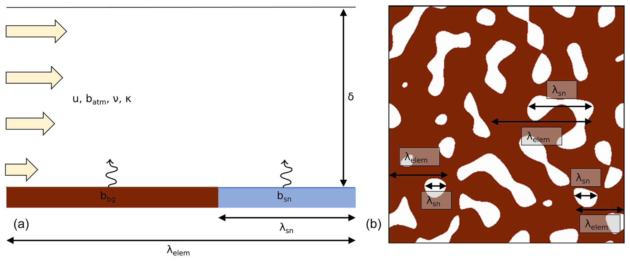
Figure 2 Conceptual situation sketches. Sketches of one snow patch and the adjacent bare ground (i.e., an element) (a) and an exemplary horizontal domain with indicated element and snow patches (b). The parameters represent the viscosity ν, thermal diffusivity κ, wind speed u, height of the atmospheric surface layer δ, average size of one snow patch element λ_elem (consisting of the length of the snow patch λ_sn and the adjacent bare ground: ${\mathit{\lambda }}_{\mathrm{elem}}\equiv {\mathit{\lambda }}_{\mathrm{bg}}+{\mathit{\lambda }}_{\mathrm{sn}}$), and the buoyancies of the snow b_sn and the bare ground b_bg.

3 Idealized system

3.1 System description

We used an idealized system (Fig. 2) to study the turbulent heat fluxes in detail and understand the behavior observed in the field. As this is one of the first studies to use DNS to investigate the role of the vertical turbulent heat fluxes and local heat advection in these systems, we focus on the sensible heat flux, even though MicroHH allows us to include the latent heat flux (e.g., Bonekamp et al., 2020). Instead of using our own measurements, the idealized system is based on the measurements of a single snow patch done by Harder et al. (2017), due to the availability of relatively high-resolution measurements and the similarity to an idealized system in which the contribution of the local-scale advection of the sensible and latent heat to the total melt is relatively large. We are aware that this complicates the comparison between our observations and simulations. The prescribed conditions within simulations of the idealized system are based on the observations of Harder et al. (2017) and obtained through a dimensional analysis (elaborated on in Sect. 3.2). We assume that our idealized system consists of, on average, a near-neutral atmosphere above a patchy surface with heterogeneous properties and can be described by the following variables:

$$\begin{array}{}\text{(3)}& \left(\mathit{\nu },\mathit{\kappa },u,\mathit{\delta },{\mathit{\lambda }}_{\mathrm{elem}},{\mathit{\lambda }}_{\mathrm{sn}},b_{\mathrm{sn}},b_{\mathrm{bg}}\right).\end{array}$$

The viscosity ν (m² s⁻¹), thermal diffusivity κ (m² s⁻¹), and wind speed u (m s⁻¹) describe the properties of the neutral atmosphere. δ (m) is the height of the atmospheric surface layer, λ_elem (m) represents the average size of one snow patch element, consisting of the snow patch itself (λ_sn) and the adjacent bare ground (${\mathit{\lambda }}_{\mathrm{elem}}\equiv {\mathit{\lambda }}_{\mathrm{bg}}+{\mathit{\lambda }}_{\mathrm{sn}}$). The buoyancies of the surface layer over the snow (b_sn) and the bare ground (b_bg) are defined as

$$\begin{array}{}\text{(4)}& b\equiv {\displaystyle \frac{g}{{\mathit{\theta }}_{\mathrm{atm}}}}(\mathit{\theta }-{\mathit{\theta }}_{\mathrm{atm}}),\end{array}$$

in which g (m s⁻²) is the gravitational acceleration, θ_atm (K) is the temperature of the atmosphere, and θ is, in our case, the temperature of snow, bare ground or atmosphere to be recalculated to the buoyancy b in this equation. This definition causes the temperature dimension to cancel out and m s⁻² to remain as the unit. In the simulations, we assumed for each simulation that the simulated atmosphere is initially well mixed, such that the temperature of the atmosphere is constant with height (similar to Harder et al., 2017). Furthermore, we assumed that the horizontal extent is orders of magnitude larger than the elements so that this does not have an influence on the physics in the model.

To assess the impact of the snow patch size, we varied λ_sn in our simulations. Specifically, we doubled and quadrupled λ_sn compared to a reference simulation with 15 m long snow patches, similar to Harder et al. (2017). Therefore, in the remainder of this paper, we will denote the reference simulation by P15m and the simulations with a doubled and a quadrupled snow patch size as P30m and P60m, respectively. The patches in P60m simulation (and some larger patches in the P30m simulation) can be compared with our own observations to study the dominant processes. Although the meteorology in the simulations is not based on the field observations, it allows for a qualitative analysis of the processes.

Furthermore, an additional simulation is performed in which the system is the same as in the P15m simulation except that stability effects are excluded. This allows us to identify the influences of stability on the vertical sensible heat fluxes, as well as the dominant turbulent character. In this simulation, temperature does not influence the buoyancy of the air. To refer to this simulation in figures, we append “NB” (i.e., the abbreviation for “No Buoyancy”) to the name, i.e., P15m-NB.

3.2 Dimensional analysis

3.2.1 Parameter derivation

To​​​​​​​ create a system physically similar to the measurements done by Harder et al. (2017) within our modeling domain, a dimensional analysis is performed according to Buckingham's Pi theorem (Buckingham, 1914). The modeling domain in which we fit these measurements is based on the atmospheric turbulent channel flow from Moser et al. (1999).

All of the descriptive variables (Sect. 3.1) are nondimensionalized by using δ and u as repeating variables, since these cover both the primary dimensions: [L] and [L T⁻¹], respectively, and are constant throughout all the numerical experiments (Sect. 3.4). This results in six dimensionless groups, which can be combined into

$$\begin{array}{}\text{(5)}& \left({\displaystyle \frac{\mathit{\nu }}{\mathit{\kappa }}},{\displaystyle \frac{u\mathit{\delta }}{\mathit{\nu }}},{\displaystyle \frac{{\mathit{\lambda }}_{\mathrm{sn}}^{\mathrm{2}}}{{\mathit{\lambda }}_{\mathrm{elem}}^{\mathrm{2}}}},{\displaystyle \frac{\mathit{\delta }}{{\mathit{\lambda }}_{\mathrm{elem}}}},-{\displaystyle \frac{b_{\mathrm{sn}}\mathit{\delta }}{u^{\mathrm{2}}}},-{\displaystyle \frac{b_{\mathrm{bg}}\mathit{\delta }}{u^{\mathrm{2}}}}\right).\end{array}$$

The nondimensional parameters can be interpreted as follows:

• $\frac{\mathit{\nu }}{\mathit{\kappa }}$ is the Prandtl number (Pr). This is assumed to be constant throughout this study, such that the flow over the patchy surface always has the same characteristics and does not influence the outcome of the simulations. In this study, the number is set to 1 instead of 0.71, which is the atmospheric value. This deviation has negligible impacts on the flow and allows for simpler scaling when analyzing the simulations (Kawamura et al., 1998).

• $\frac{u\mathit{\delta }}{\mathit{\nu }}$ is the Reynolds number (Re). For the same reason as the Prandtl number, this parameter is taken to be constant throughout the study. During this study, the same Reynolds number as in Moser et al. (1999) is taken: 1.10×10⁴. Therefore, we impose a wind speed of 0.11 m s⁻¹, a 1 m vertical extent, and a viscosity of $\mathrm{1.0}\times {\mathrm{10}}^{-\mathrm{5}}$ m² s⁻¹.

• $\frac{{\mathit{\lambda }}_{\mathrm{sn}}^{\mathrm{2}}}{{\mathit{\lambda }}_{\mathrm{elem}}^{\mathrm{2}}}$ is the snow cover fraction (SCF) and varies between zero and 1. If this parameter is 1, the field is completely snow covered, whereas values close to zero represent low snow-cover fractions. For all simulations, this dimensionless group is set to a value of 0.25, similar to Schlögl et al. (2018a), as Harder et al. (2017) does not provide any information about this.

• $\frac{\mathit{\delta }}{{\mathit{\lambda }}_{\mathrm{elem}}}$ is a measure of the size of a surface element compared to the height of the system. This nondimensional number will decrease if the typical element size increases. If the snow cover fraction is kept constant, changes in this variable will affect the typical snow patch size, meaning that this variable can be interpreted as a measure of the relative snow patch size.

• $-\frac{b_{\mathrm{sn}}\mathit{\delta }}{u^{\mathrm{2}}}$ is the bulk Richardson number above the snow patches (Ri_sn). Positive and negative values indicate, respectively, stability and instability, whereas the absolute values specify the magnitude of the (in)stability.

• $-\frac{b_{\mathrm{bg}}\mathit{\delta }}{u^{\mathrm{2}}}$ is the bulk Richardson number above the bare ground (Ri_bg). For Ri_bg, the same principles hold as for Ri_sn.

We ensure that the increases in snow patch size λ_sn that are necessary for our analysis only affect the relative element size $\frac{\mathit{\delta }}{{\mathit{\lambda }}_{\mathrm{elem}}}$. We do this by changing λ_sn in tandem with λ_elem such that the snow cover fraction $\frac{{\mathit{\lambda }}_{\mathrm{sn}}^{\mathrm{2}}}{{\mathit{\lambda }}_{\mathrm{elem}}^{\mathrm{2}}}$ remains constant. This allows us to study the impact of increasing the snow patch size separately from the snow cover fraction.

3.2.2 Parameter estimation

The measurements of Harder et al. (2017) are first used to calculate the values of the defined dimensionless parameters (Table 1). Note that not all values of the variables used in the dimensionless parameters are known and are therefore estimated based on other literature, such as Schlögl et al. (2018a) (Table 2). Subsequently, the values of the variables from Moser et al. (1999) are filled into the nondimensional parameters so that the remaining dimensionless parameters can be calculated for all simulations.

It should be noted that, for the P60m simulation, the nondimensional number $\frac{\mathit{\delta }}{{\mathit{\lambda }}_{\mathrm{elem}}}$ is rather low and could potentially affect the outcomes. During this simulation, the number is 0.83, whereas the number was originally designed to be approximately 1 or higher so that the relative snow patch size would not be too large. The implications of this could be that the largest turbulent structures arising due to the snow patches do not have enough space to develop and are therefore affected by the horizontal domain of the simulation. However, the results show no clear deviations from the expectation, and thus we assume that the influence of this value of the nondimensional number is relatively minor to nonexistent.

Table 1 Dimensionless parameter values. Overview of the values of the dimensionless parameters applied during the simulations.

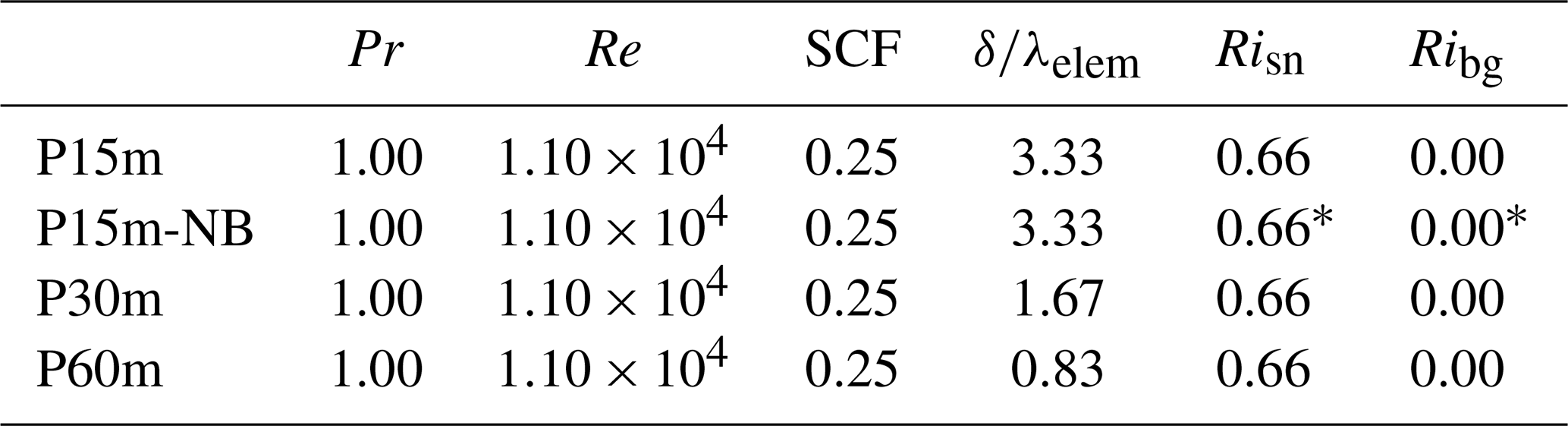
^* These are not, in fact, real Richardson numbers, as buoyancy does not affect the flow in the P15m-NB simulation.

Harder et al. (2017)Moser et al. (1999)

Table 2 Variable values applied in the simulations. Overview of the values used for obtaining the dimensionless parameters in the simulations.

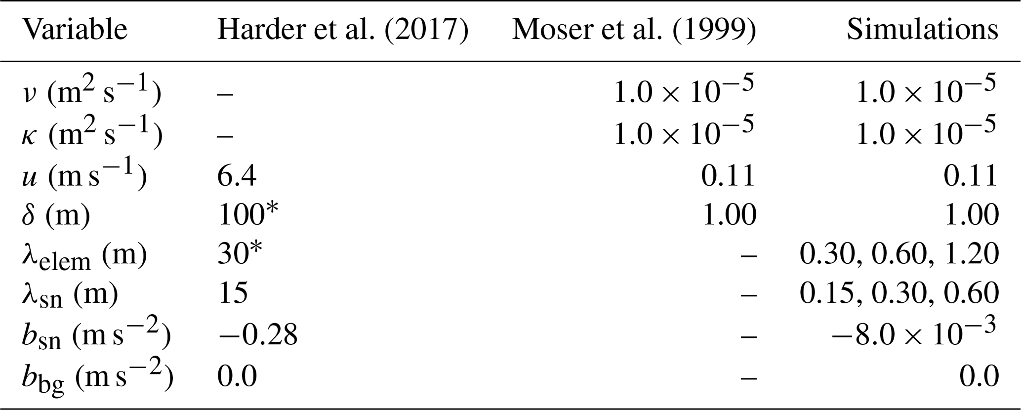
^* Values were estimated based on Schlögl et al. (2018a).

3.3 Rescaling the model results to reality

After nondimensionalizing the system for the simulations, the outcomes of the simulations are rescaled back to realistic scales to compare with the observations. In order to do so, the nondimensional numbers are used, as these numbers characterize the dominant processes in the considered idealized system.

When rescaling the surface heat fluxes back to reality, Ri_sn influences the rescaling factor that is used. This factor indicates whether shear-driven turbulence or buoyancy-driven turbulence or a balance between the two is more dominant in the system, and thus also which process predominantly affects the surface buoyancy flux scaling. We assume shear-driven turbulence to be dominant near the surface, such that the rescaling equation becomes

$$\begin{array}{}\text{(6)}& B_{\mathrm{0}}=u{b}_{\mathrm{sn}},\end{array}$$

in which B₀ is the typical buoyancy surface flux (m² s⁻³), b_sn is the surface buoyancy of snow (m s⁻²), and u is the wind speed (m s⁻¹). This equation is derived from the original equation for surface buoyancy flux implemented in the model

$$\begin{array}{}\text{(7)}& \begin{array}{rl}{B}_{\mathrm{0}}& =-{\left.\mathit{\kappa }{\displaystyle \frac{\partial b}{\partial z}}\right|}_{\mathrm{sn}}\approx -{\left.\mathit{\kappa }{\displaystyle \frac{\mathit{\delta }b}{\mathit{\delta }z}}\right|}_{\mathrm{sn}},\\ & \sim \mathit{\kappa }{\displaystyle \frac{b_{\mathrm{sn}}}{{\mathit{\delta }}_{\mathrm{v}}}},\end{array}\end{array}$$

in which δ_v is the depth of the viscous sublayer (m), which is assumed to be of the same order of magnitude as δz, whereas b_sn is assumed to be a measure of δb. For δ_v, we use the viscous sublayer instead of the boundary layer, as the latter is approximately neutral, such that buoyancy is constantly zero throughout the layer except near the surface.

Equation (8) follows from a definition of the height of the viscous sublayer δ_v for conditions in which shear dominates, such that δ_v is determined by the wind and viscosity. This allows us to set up a relation between these three variables:

$$\begin{array}{}\text{(8)}& \begin{array}{rl}{\mathit{\delta }}_{\mathrm{v}}& =f(u,\mathit{\nu }),\\ & \sim {\displaystyle \frac{\mathit{\nu }}{u}}.\end{array}\end{array}$$

Implementing this in Eq. (7) gives Eq. (6):

$$\begin{array}{}\text{(9)}& B_{\mathrm{0}}\sim \mathit{\kappa }{\displaystyle \frac{b_{\mathrm{sn}}}{\left(\frac{\mathit{\nu }}{u}\right)}}=\mathit{\kappa }u{\displaystyle \frac{b_{\mathrm{sn}}}{\mathit{\nu }}}=u{b}_{\mathrm{sn}},\end{array}$$

as κ and ν cancel out since Pr (i.e., $\frac{\mathit{\nu }}{\mathit{\kappa }}$) is unity in this study. Subsequently, this equation can be used to rescale the simulated surface buoyancy fluxes back to realistic values according to

$$\begin{array}{}\text{(10)}& {\displaystyle \frac{B_{\mathrm{0},\mathrm{sim}}}{B_{\mathrm{0},\mathrm{real}}}}={\displaystyle \frac{u_{\mathrm{sim}}{b}_{\mathrm{sn},\mathrm{sim}}}{u_{\mathrm{real}}{b}_{\mathrm{sn},\mathrm{real}}}}.\end{array}$$

From Table 2, it follows that $b_{\mathrm{sn},\mathrm{sim}}=-\mathrm{0.008}$ m s⁻², $b_{\mathrm{sn},\mathrm{real}}=-\mathrm{0.28}$ m s⁻², u_sim=0.11 m s⁻¹, and u_real=6.4 m s⁻², so the equation reduces to

$$\begin{array}{}\text{(11)}& {\displaystyle \frac{B_{\mathrm{0},\mathrm{sim}}}{B_{\mathrm{0},\mathrm{real}}}}={\displaystyle \frac{\mathrm{0.11}\times -\mathrm{0.008}}{\mathrm{6.4}\times -\mathrm{0.28}}}=\mathrm{4.9}\times {\mathrm{10}}^{-\mathrm{4}}.\end{array}$$

Thus, the simulated values for the surface buoyancy fluxes are divided by $\mathrm{4.9}\times {\mathrm{10}}^{-\mathrm{4}}$ to compute the realistic values.

Subsequently, the outcome for the realistic surface heat fluxes can be transformed into W m⁻² according to

$$\begin{array}{}\text{(12)}& H_{\mathrm{real}}=\mathit{\rho }{c}_{\mathrm{p}}{\displaystyle \frac{{\mathit{\theta }}_{\mathrm{0}}}{g}}{B}_{\mathrm{real}},\end{array}$$

in which H is the sensible heat flux into the surface (W m⁻²), ρ is the density of the air (kg m⁻³), c_p is the specific heat capacity (J kg⁻¹ K⁻¹), θ₀ is the reference temperature (273 K in this case), and g the gravitational acceleration (m s⁻²).

To rescale the simulated time back to reality, the bulk Richardson number above snow (${\mathit{Ri}}_{\mathrm{sn}}=-\frac{b_{\mathrm{sn}}\mathit{\delta }}{u^{\mathrm{2}}}$) is used for obtaining the timescale. From this number, the following timescale is derived:

$$\begin{array}{}\text{(13)}& {\displaystyle \frac{\mathit{\delta }}{u}}=t_{\mathrm{adv}},\end{array}$$

in which t_adv (s) resembles an advective timescale.

When calculating the ratios between the simulated and measured timescales by making use of the values in Table 2, the following ratio between the simulated and realistic timescales arises:

$$\begin{array}{}\text{(14)}& {\displaystyle \frac{t_{\mathrm{adv},\mathrm{sim}}}{t_{\mathrm{adv},\mathrm{meas}}}}={\displaystyle \frac{\mathrm{9.09}}{\mathrm{15.63}}}=\mathrm{0.58}.\end{array}$$

Thus, the simulated time is divided by 0.58 to compute the realistic value.

3.4 Model description and setup

In this study, the model simulations are performed using the MicroHH 2.0 code, which was primarily made for the DNS of atmospheric flows over complex surfaces by van Heerwaarden et al. (2017). When solving the conservation equations for mass, momentum, and energy, MicroHH makes use of the Boussinesq approximation, such that the evolution of the system for a velocity vector with element u_i, buoyancy b, and volume is described by

$$\begin{array}{}\text{(15)}& \begin{array}{rl}{\displaystyle \frac{\partial u_i}{\partial t}}+{\displaystyle \frac{\partial u_j{u}_i}{\partial x_j}}& =-{\displaystyle \frac{\partial \mathit{\pi }}{\partial x_i}}+{\mathit{\delta }}_{i\mathrm{3}}b+\mathit{\nu }{\displaystyle \frac{{\partial }^{\mathrm{2}}{u}_i}{\partial x_j^{\mathrm{2}}}},\\ {\displaystyle \frac{\partial b}{\partial t}}+{\displaystyle \frac{\partial u_{j}b}{\partial x_j}}& =\mathit{\kappa }{\displaystyle \frac{{\partial }^{\mathrm{2}}b}{\partial x_j^{\mathrm{2}}}},\\ {\displaystyle \frac{\partial u_j}{\partial x_j}}& =\mathrm{0},\end{array}\end{array}$$

in which π is a modified pressure (van Heerwaarden and Mellado, 2016). Moreover, MicroHH uses periodic boundary conditions in the horizontal directions, which implies that we simulate a wind blowing over an infinite snow field. In the following parts of the article, when we report vertical sensible heat fluxes into the surface, these were recalculated from the surface buoyancy flux B (m² s⁻³) computed in the model equation according to

$$\begin{array}{}\text{(16)}& B=-{\left.\mathit{\kappa }{\displaystyle \frac{\partial b}{\partial z}}\right|}_{\mathrm{surface}},\end{array}$$

which can be recalculated to give realistic sensible heat fluxes following the steps in Sect. 3.2. Similarly to Harder et al. (2017) (Eq. 2), the horizontally advected sensible heat is computed via

$$\begin{array}{}\text{(17)}& H_{\mathrm{adv}}=\underset{z=\mathrm{0}\mathrm{m}}{\overset{z=\mathrm{2}\mathrm{m}}{\int }}\mathit{\rho }{c}_{\mathrm{p}}\stackrel{\mathrm{‾}}{u}{\displaystyle \frac{\partial \stackrel{\mathrm{‾}}{\mathit{\theta }}}{\partial x}}\mathrm{d}z,\end{array}$$

in which z (m) is the elevation above the surface, ρ (kg m⁻³) is the air density, c_p (1005 J kg⁻¹ K⁻¹) is the specific heat capacity of air, and x (m) is the distance from the leading edge of the snow patch. As well as integrating over a 2 m profile height, we also integrate over a 4 m height.

The starting point for designing the numerical experiments is the atmospheric turbulent channel flow with a reduced Reynolds number (Re) designed by Moser et al. (1999). This simulation is also used as a spin-up, during which we have no buoyancy effects included in the flow. The shear Reynolds number Re_τ obtained from the measurements performed by Harder et al. (2017) is relatively high compared to that of Moser et al. (1999): $\sim \mathrm{6}\times {\mathrm{10}}^{\mathrm{6}}$ vs. 590, but the results of Moser et al. (1999) suggest that the bulk statistics, i.e., the means and variances, for at least the initial neutral channel flow are hardly affected Re_τ. This channel flow is simulated in MicroHH at a resolution of 384 × 192 × 128 grid points for a domain size of 2π m × π m × 2 m. The flow is forced in the x direction by imposing an average wind speed, which is, in this case, 0.11 m s⁻¹. At the bottom and top boundaries, no slip and no penetration conditions are applied to the velocities (i.e., the flow velocity at the boundary is zero). Overall, van Heerwaarden et al. (2017) showed that MicroHH is able to reproduce this turbulent channel flow.

Initially, the turbulent channel flow from Moser et al. (1999) used as a spin-up is simulated until 1800 s so that the turbulent channel flow is well developed. Subsequently, for each simulation, which takes 900 s, this turbulent channel flow is adapted such that an atmospheric flow over a patchy snow surface is obtained. At the bottom boundary, a pattern of surface buoyancies that depends on the simulation is prescribed, such that the surface characteristics determined during the dimensional analysis are fulfilled. For snow and bare ground, the surface buoyancy is respectively $-\mathrm{8}\times {\mathrm{10}}^{-\mathrm{3}}$ and 0.0 m s⁻² (i.e., 273 and 280.9 K in reality), which is elaborated on in Sect. 3.2. The implemented surface for P15m and P15m-NB (P30m, P60m) contains snow patch lengths of 0.15 m (0.30 m, 0.60 m) on average, and average element lengths of 0.30 m (0.60 m, 1.20 m) (Table 2; multiplied with 100 in Fig. 3). These surfaces enable the model to solve the periodic boundary conditions, because we ensure that the patches at opposing walls fit together and that flow that leaves the system on one side continues over the same snow patch when it reenters the system on the opposite wall. These patterns are created by generating noise in the Fourier space around specific wavelengths, prescribed in the form of 2D power spectra. When transforming these back to physical space using the inverse fast Fourier transform, a 2D field with dominant patterns is obtained. For a more elaborate explanation of generation, see Appendix B.

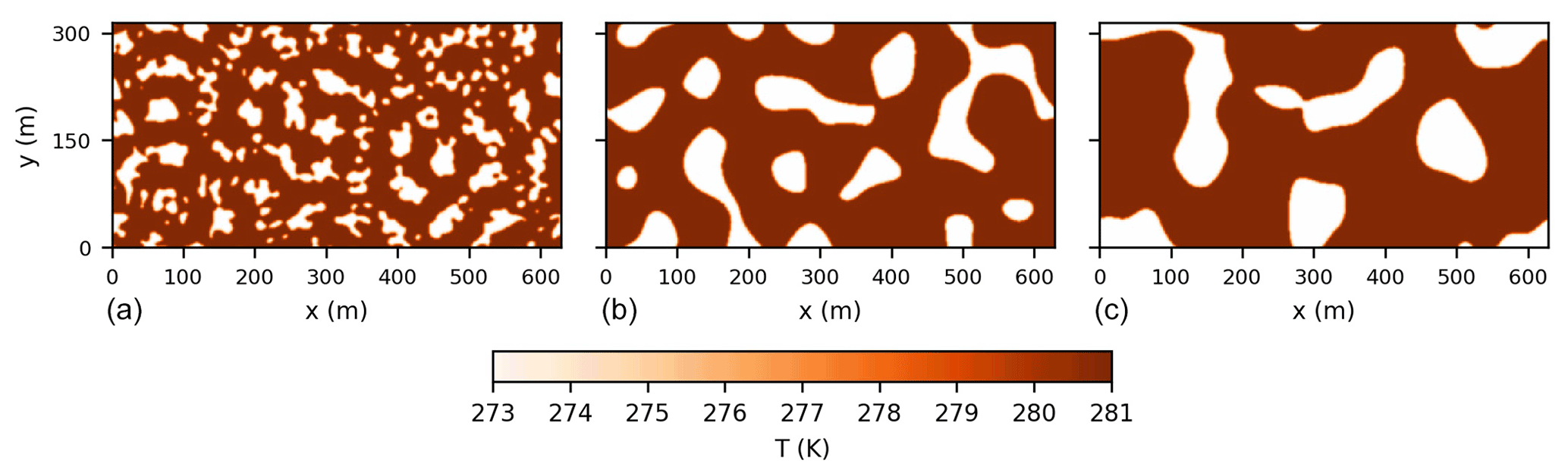
Figure 3 Generated realistic surface temperatures for the P15m and P15m-NB (a), P30m (b), and P60m (c) simulations.

4 Field observations

At the upwind edge of the snow patch, the snow surface decreased by approximately 23 cm, whereas for the downwind edge, this decrease was approximately 3 cm (Fig. 4). For the upwind edge, the height change is computed relative to 11 June 17:00 LT. For the downwind edge, the height change is computed relative to 12 June 16:00 LT, due to a low coverage of bare ground pixels on 11 June (Fig. A1), which are used for computing the vertical correction employed to align all height maps (Table 3). For the upwind edge, the melt relative to 12 June 16:00 LT is estimated to be 21 cm.

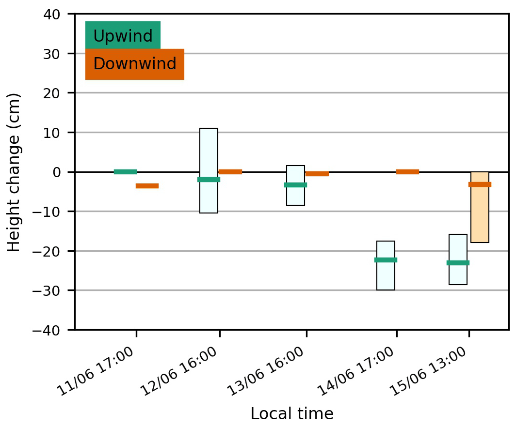
Figure 4 Boxplot of height changes for the upwind and downwind edges of a snow patch recorded with SfM photogrammetry from 11 June 2019 until 15 June 2019. For the upwind edge, 11 June is taken as the reference date. For the downwind edge, the first measurement on 11 June is not used as the reference, due to a low coverage of grid cells. The melt is estimated with an error of ±2.0 and ±0.4 cm, respectively, for the upwind and downwind edges.

The average standard error after applying the vertical correction for the bare ground grid cells that are present throughout the all height maps is 1.38 cm for the upwind edge and 0.29 cm for the downwind edge. The propagation of these errors ($\sqrt{\mathrm{2}{\mathit{\sigma }}_{\mathrm{\Delta }\stackrel{\mathrm{‾}}{h}}^{\mathrm{2}}}$), which is caused by relating the height changes in two height models, allows us to estimate the melt with an error of ±2.0 and ±0.4 cm, respectively, for the upwind and downwind edges. Usually, these standard errors are calculated over other grid cells rather than those used for the vertical correction, such that these points are independent. In this study, however, the standard error and vertical correction are computed for all bare-ground grid cells present throughout the research period, since the relatively small spatial scale causes all grid cells to be related. Considering the errors, for the upwind edge, significant melt was recorded on 13 June and onwards as compared to 11 June, used as reference. For the downwind edge, significant melt was recorded on 13 and 15 June, taking 12 June as reference. For the third period from 13 to 14 June, an increase in snow height relative to the previous day was recorded, but this increase was not significant due to overlapping error estimates.

Table 3 Vertical shift correction (cm) applied in the individual height models per day for the upwind and downwind locations.

^* Only computed with the bare ground grid cells present in this height map.

4.1 Relation between snowmelt and meteorology

Relating the meteorological circumstances (Table 4) to the measured snowmelt allows us to estimate the contribution of the vertical turbulent heat fluxes to the total amount of snowmelt. To do so, the snow density measurements are used. The snow densities at 5, 25, and 45 cm below the snow surface are, respectively, 556, 551, and 610 kg m⁻³. It follows from these densities that the snow density is approximately constant near the surface, whereas the snow is more compressed or stores water further down. Even though these densities are relatively high, we consider the values to be realistic considering that the largest discharge peak took place 1.5 months before the observation period (Fig. 1) and given the observation that the snowpack was relatively wet in the field.

Table 4 Average meteorological measurements and calculated variables in between the photogrammetry observations. T_2 m is the air temperature measured at 2 m; u_10 m and u_dir are, respectively, the wind speed and wind direction in degrees from the north and measured at 10 m; P_r is the summed precipitation during the period; SW^↓ and LW^↓ are, respectively, the incoming shortwave and longwave radiation; RH_2 m is the measured relative humidity at 2 m; and P_a is the air pressure. The net radiation (R_net), subsequent melt (M_R), and specific humidity difference (q−q_sn) were computed based on a combination of the measured variables. The ranges for R_net and M_R are caused by applying two values for the albedo, i.e., 0.6 and 0.8, to account for uncertainties in the shortwave radiation component (see Sect. 2).

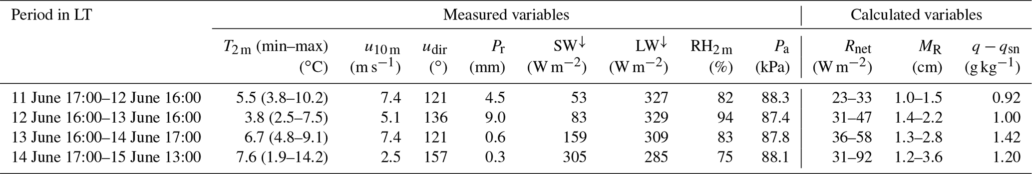
The minimum estimated melt due to net radiation from 12 June until 15 June was 3.9 cm (Table 4), which is 0.5 cm larger than the melt estimate including the error for the downwind edge. As the snow patch was approximately 50 m in length, the turbulent heat fluxes into the snow likely reduced to negligible values at the downwind edge (e.g., when extrapolating the measurements of Harder et al., 2017), so this mismatch is most likely caused by uncertainties in the net radiation estimates. When assuming this radiation to be an appropriate estimate and that it is homogeneously spread over the patch, the estimated contribution of the vertical turbulent heat fluxes at the upwind edge is 13.0 to 18.2 ± 2.0 cm. For this, we also assume that the residual of the difference between the observed snowmelt and radiation-driven snowmelt is caused by these turbulent heat fluxes (e.g., Plüss and Mazzoni, 1994). When using Eq. (2) to compute the average vertical turbulent heat fluxes during the period, we estimate these fluxes at the upwind edge to be between 73 and 102 ± 11 W m⁻². These are of the same order as those found in other studies in somewhat similar conditions, such as Mott et al. (2018), Olyphant and Isard (1988), and Harding (1986). Mott et al. (2018) reported a sensible heat flux into the snow of up to 50 W m⁻² for typical weather situations in alpine areas, whereas the latent heat was negligible or even contributed to the cooling of the snow. Olyphant and Isard (1988) reported downward turbulent heat fluxes of over 100 W m⁻² for a large single snow patch. Harding (1986) estimated the full energy balance for 15 d in May of a relatively homogeneous snow cover near Finse and reported a sensible heat flux of approximately 20 W m⁻² and a latent heat flux that was negligible on average. For our observations, however, it is expected the latent heat flux also had a significant contribution from the high relative humidity, with a subsequent difference in specific humidity between the air and snow of at least 0.9 g kg⁻¹ (Table 4) during the field campaign, which is common for Finseelvi as it is located in a maritime climate. Our results show similar moisture gradients to Harder et al. (2017), who found a significant influence of the latent heat on the snowmelt, such that we expect this to be a significant part of our estimated turbulence-driven melt. Overall, by comparing the overall melt with the melt driven by the radiation and taking the residual as the turbulence-driven melt, we estimate the contribution of the turbulent heat fluxes to the snowmelt to be roughly 60 to 80 % for the upwind edge of the snow patch. Extrapolating this to the entire catchment and applying the relations reported by Schlögl et al. (2018b) for two test sites in the Alps, we estimate the contribution of the fluxes to the total melt to be maximally on the order of 10 % under the assumption that the entire catchment behaves similarly.

It is likely that the incoming radiation for the entire snow patch is overestimated, due to topography. The incoming solar radiation at the snow patch is blocked by mountains at low solar angles in the east and west, which does not apply at the location of the meteorological observations. Moreover, the incoming longwave radiation reduces with height, as was found in the Alps by Marty et al. (2002), such that this snow patch – located 150 m higher – received less incoming longwave radiation. Lastly, other characteristics influencing the net radiation, such as a varying snow albedo and slightly different slopes for the upwind and downwind edges, are also identified as potential influences on the results.

5 Model simulations

5.1 System characteristics

In the idealized simulations, the time-averaged sensible turbulent heat fluxes resemble the implemented surface pattern of snow patches (Fig. 5). There is a negative surface flux on the snow patches, whereas the surface flux is positive at the bare ground. For each snow patch, there is a clear pattern that is somewhat similar to the observations. The leading edge of the snow patch shows the highest fluxes towards the surface, $\sim -\mathrm{500}$ W m⁻², which decreases downwind of the leading edge until the end of the patch. Subsequently, at the trailing edge of the snow patch and the leading edge of the bare ground, the sensible heat flux changes sign, as the bare ground is relatively warm compared to the colder air coming from above the snow patch, resulting in ∼300 W m⁻². The air warms when flowing over the bare ground, such that the air arriving at the next snow patch is relatively warm compared to that at the cold snow patch, causing a high downward flux. These fluxes at the leading edges of the snow patches are relatively high, mostly due to the presence of ideal circumstances for wind-driven melt, including local-scale advection of sensible heat (i.e., high wind speeds and relatively large temperature differences). Compared to our own observations, the sensible heat fluxes at the leading edge are much larger than the observed combined turbulent heat fluxes. This is in line with our expectations because of the inclusion of nonideal circumstances for local-scale advection of the sensible and latent heat during the field campaign.

Figure 5 Time-averaged surface sensible turbulent heat fluxes. Sensible turbulent heat fluxes in the P15m simulation averaged from 2000 seconds until 2700 s. Negative values indicate a downward flux, i.e., over snow patches, whereas positive values resemble an upward flux, i.e., over bare ground.

5.2 Total snowmelt

When comparing the average sensible heat fluxes for all the snow patches in the domain, clear differences arise between all simulations (Fig. 6). The highest sensible heat fluxes towards the snow (i.e., the most negative fluxes) are found in the simulation without buoyancy effects. This also causes the total sensible heat flux in this simulation to be significantly lower than in the other simulations. Furthermore, increasing the snow patch size reduces the heat fluxes into the snow patches. The heat fluxes of the simulation with a doubled snow patch size (P30m) are decreased by approximately 15 % relative to the P15m simulation. For the simulation with a quadrupled snow patch size (P60m), the heat fluxes are reduced by approximately 25 %. This is in contrast to the results of Schlögl et al. (2018a), who report only a minor influence of snow patch size on the amount of melt. Our findings are more in line with the results of Marsh et al. (1999), who based their work on a 2D boundary layer model with a regular tiled surface pattern. Potentially, the differences from Schlögl et al. (2018a) are caused by the inability of ARPS to fully resolve the leading edge effect, as the resolution is too coarse to resolve the thin internal stable boundary layer formed over snow patches and the Monin–Obukhov assumptions are violated. Neither of these limitations apply for DNS.

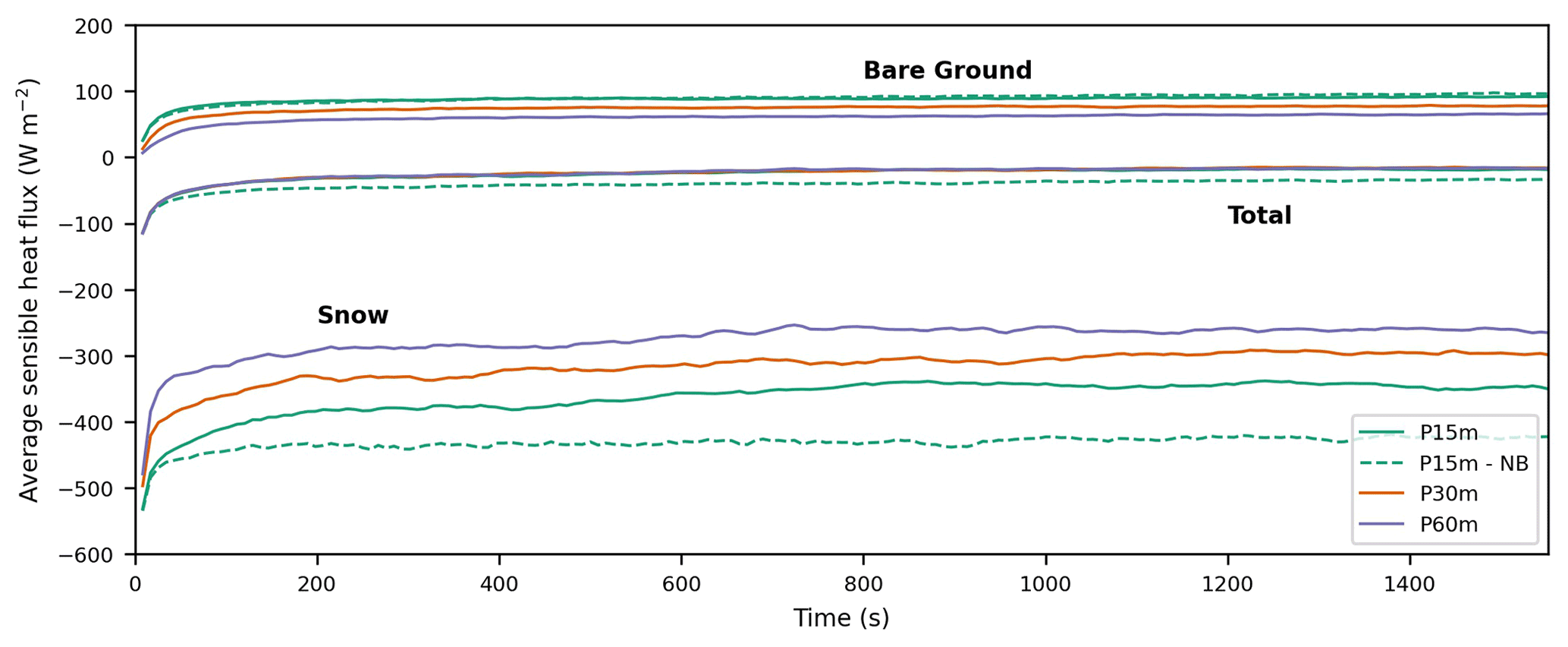
Figure 6 Domain-averaged sensible heat fluxes for different surfaces. The figure shows time series of the averaged surface sensible heat fluxes for the bare ground, snow, and total surface after the introduction of the temperature differences at the surface.

The total heat fluxes for the simulations with 15, 30, and 60 m snow patches coincide approximately, as the differences arising at the snow surface are compensated for at the bare ground surface. So, although the total fluxes are equal, the snowmelt does vary with snow patch size. The simulation without buoyancy effects (P15m-NB) has a significantly reduced total heat flux compared to the original simulation (P15m). This is caused by similar averaged heat fluxes for the bare ground for both simulations, whereas this is not the case above the snow patches. This suggests that stability has little effect on the fluxes above the bare ground, whereas the surface heat fluxes above the snow are affected by stability.

Moreover, the largest adjustment of the sensible heat fluxes after the initiation of the simulations is done after less than 200 s. However, a minor long-term trend is still present for each simulation. For this study, we assume that after the largest adjustment, the dominant processes are well developed and suffice to understand the system. We expect that, eventually, the total summed surface sensible heat fluxes will go to zero, due to the infinite blowing of the air over the snow cover without any other heat fluxes than those originating from the snow patches and bare ground. However, as the volume of the channel is relatively large compared to the heat fluxes, it takes a relatively long time before the whole system has cooled and reached an equilibrium.

5.3 Surface fluxes for individual patches

The surface fluxes for all individual snow patches in each simulation show a similar behavior over distance from the leading edge, but differences occur above snow patches due to varying fluxes at the leading edge (Fig. 7). The linear behavior of the surface fluxes as a function of the distance from the upwind edge on logarithmic axes implies that the fluxes decay over distance from the leading edge according to a power law. The power laws take the following approximate forms:

$$\begin{array}{}\text{(18)}& H_{\mathrm{sn}}\left(x\right)\equiv C_{\mathrm{sn}}{x}^{-\mathrm{0.35}},\end{array}$$

in which H_sn (W m⁻²) is the sensible heat flux, x (m) is the distance from the leading edge, and C (W m^−1.65​​​​​​​) is a constant representing the initial conditions at the leading edge of each patch.

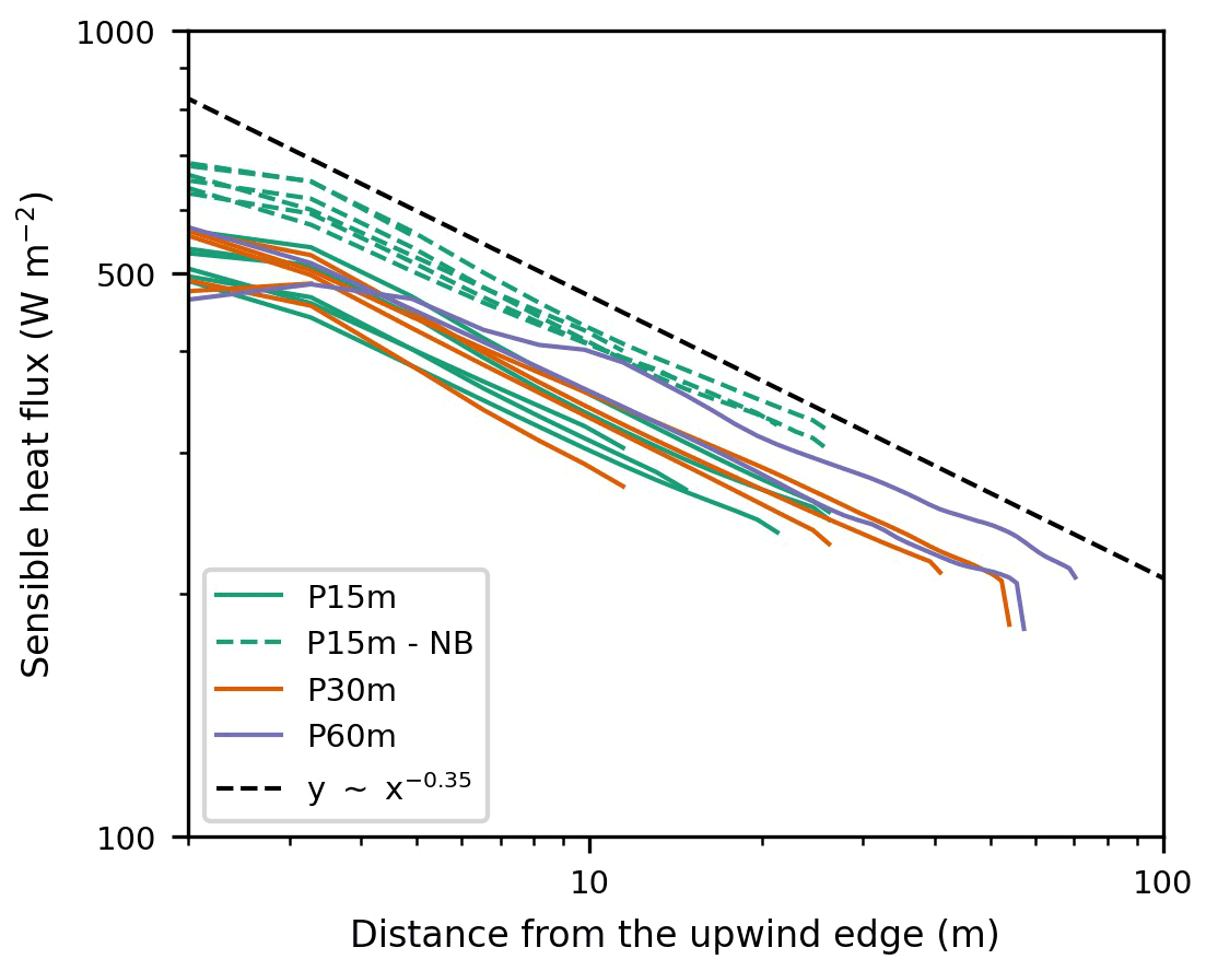
Figure 7 Time-averaged surface sensible heat fluxes over single patches of snow. The surface sensible heat fluxes for individual patches with snow as a function of distance from the leading edge on a log-log​​​​​​​ scale at y=1.1 m are shown. The dashed black line is a trendline implemented to show the approximate power law decay of the fluxes over distance. The fluxes of the snow are multiplied with −1 so that these values can also be plotted on logarithmic axes.

Our simulated vertical sensible heat fluxes into the snow are approximately 500 W m⁻² at the upwind edge and 200–300 W m⁻² at the downwind edge. In comparison to our field observations, these sensible heat fluxes at both edges are relatively high. At the upwind edge, the simulated sensible heat fluxes are approximately 5 times larger than the derived contribution of the combined turbulent heat fluxes to the measured snowmelt. We reckon that the simulated values are large, though it should be noted that the simulations are based on highly ideal conditions for turbulence-driven melt and local-scale advection of sensible and latent heat, whereas the conditions during the measurements were not ideal (e.g., nighttime melt was included). At the downwind edge, the measurements suggest an approximately negligible contribution of the vertical turbulent heat fluxes to the snowmelt, whereas, at comparable snow patches, the simulations show a significant contribution of the sensible heat flux (∼200–300 W m⁻²). Thus, the simulated decay of the sensible heat flux seems to be an underestimation in comparison to field observations. We expect that the comparable behavior of the sensible heat fluxes between patches within the idealized system is also occurring within the Finseelvi catchment for patches within similar local conditions.

Figure 7 shows that the length of snow patches is the main cause of less snowmelt for larger patches, which was also found by Marsh et al. (1999). The power laws are approximately the same for each patch and simulation, whereas C_sn is the same for each simulation except in the simulation without buoyancy effects. This behavior explains why larger snow patches reduce the average surface fluxes into the snow patches.

The behavior of the simulation without buoyancy effects is striking, as the decay of the fluxes for this simulation is similar to the decay of the fluxes for the other simulations, suggesting that stability has little influence on the decay of the surface heat fluxes, i.e., shear turbulence dominates. However, this simulation has a relatively low initial surface flux above the snow (a higher absolute flux in Fig. 7), indicating an effect of the stability on the leading edge conditions. Thus, the differences in total snowmelt (Fig. 6) between the P15m and P15m-NB simulations solely occur due to these differences at the leading edge.

The decay of the sensible heat fluxes is a consequence of the decreasing temperature gradients in the IBL (Fig. 8a). Wind speed, another important component affecting the sensible heat flux, remains constant over a snow patch (Fig. 8b). Moreover, surface roughness is the same for the entire domain. Strikingly, the average temperature within the IBL remains constant and does not depend on the height of this IBL, as the shape of the vertical temperature profile remains constant while the flow proceeds over the snow patch (Fig. 8a inset). Yet, it should be noted that the reported values for the height of the IBL are relatively high compared to Harder et al. (2017).

Compared to Harder et al. (2017), our estimates of the horizontally advected sensible heat are relatively high. The measurements done by Harder et al. (2017) show values slightly above 400 W m⁻² for the first 3.6 m (Fig. 8c). In our simulations, the horizontal advection of sensible heat decreases in the first 3.6 m from 577 W m⁻² to approximately 400 W m⁻². For the following 4.8 m, Harder et al. (2017) reported an average reduction in horizontally advected sensible heat to approximately 20 % of the values found for the first 3.6 m. This reduction is not found in the comparable simulation with a similar dominant snow patch pattern. Yet, further downwind, the advected sensible heat does reduce to values of the same order of magnitude. It should be noted that, due to setting the integration height at 2 m in Eq. (17), not all changes in the vertical temperature profile over the distance from the leading edge are included, such that the horizontally advected sensible heat is underestimated. When considering a 4 m integration height, the horizontally advected sensible heat is approximately equal to the vertical sensible turbulent heat fluxes at the snow surface, especially for the first half of the patch, also implying a power of −0.35 for the decay of the horizontally advected sensible heat. This also illustrates the major contribution of the horizontally advected sensible heat to the sensible heat flux into the snow. We expect a similar role of the advected heat in our field observations, as there was a patchy snow cover present in all directions and at great distances from the observed snow patch, causing approximate equilibrium conditions. In comparison to a similar relationship obtained by Granger et al. (2002) (based on Weismann, 1977) through boundary-layer integration, our advected heat decays less. Granger et al. (2002) come up with a similar power law, but their powers maximally reach −0.47, depending on the surface temperatures of the snow and bare ground, the friction velocity, and the roughness length.

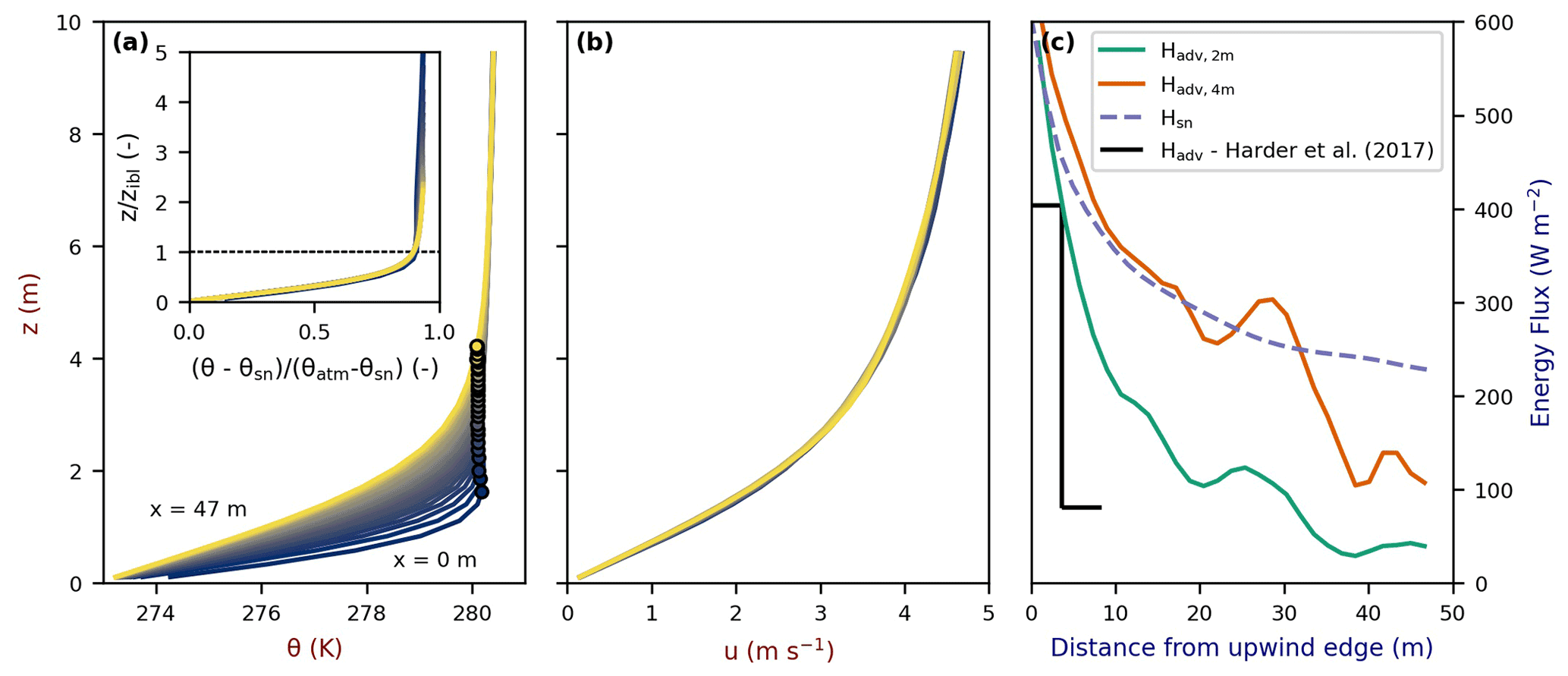
Figure 8 Time-averaged vertical temperature (a) and wind (b) profiles and horizontally advected sensible energy H_adv at 2 and 4 m integration height and vertical sensible heat flux at the surface H_sn (c) along the snow patch at y=83 m and x=150 m in the P30m simulation. The markers in the temperature profile resemble the IBL height, which is computed as the first value (seen from the bottom) of the gradient of the temperature with height below 0.1 K m⁻¹. The first two upwind grid cells and two downwind grid cells have been removed, as these are located in the transition region from bare ground to snow and vice versa. The labels with “x=” show the locations of vertical profile related to the downwind distance of the vertical profile from the leading edge, whereas the line color indicates the distance from the leading edge and goes from purple to red. In the inset graph, the vertical temperature profile has been normalized to the height of the IBL and the prescribed temperatures of the surface and atmosphere. The advected energy as a function of distance from the leading edge is based on Eq. (17).

6 Discussion

This study aimed to assess the role of local-scale advection of sensible and latent heat fluxes on snowmelt. In order to do so, complementary field observations and simulations were performed. On small spatial scales, the largest melt differences due to the combined turbulent heat fluxes occur at the opposing edges of snow patches. Our results show that the upwind edge of a single snow patch in the Finseelvi catchment, which is approximately 50 m in length, melted 23 ± 2.0 cm over the course of 5 d, whereas the downwind edge melted just 3 ± 0.4 cm in 4 d. As the snow patch was approximately 50 m long, the vertical turbulent heat fluxes likely reduced to negligible values at the downwind edge, due to the leading edge effect, such that the main cause of melt at this edge was the net radiation. The simulations allowed us to extract detailed information on the atmospheric flow and were used as a tool to provide insight into the evolution of the fluxes and temperature over the patchy snow cover. The sensible heat fluxes reduce over distance from the upwind edge, following a constant power law which likely depends on the meteorological circumstances. In the simulations, this resulted in a reduction of 15 % and 25 % for, respectively, a doubling and a quadrupling in snow patch size. The simulations reveal that the reducing sensible heat fluxes over distance from the leading edge are caused by the reducing temperature gradients, pointing out the major role of the horizontally advected sensible heat, which we expect behaved similarly in our field observations. Other important factors for the turbulent heat fluxes, i.e., wind speed and surface roughness, are constant over distance from the leading edge in the simulations.

However, the simulations lacked surface roughness differences for the snow and bare ground and topographical variations. Including the transition from a rough (bare ground) to a smooth (snow) surface would likely diminish the IBL growth due to increased turbulence levels and enhance the vertical sensible heat fluxes as a consequence of the larger temperature gradients in the IBL (Garratt, 1990). It should be noted that this mostly holds for shear-dominated turbulence, whereas at lower wind speeds, the influence of thermal turbulence on the IBL should also be considered. Moreover, the common formation of snow patches in topographical depressions causes atmospheric decoupling and reduced vertical turbulent heat fluxes at low and moderate wind speeds, especially downstream of the upwind edge (Mott et al., 2016). In the Finseelvi catchment, snow patches have formed to some extent in these depressions, while this does not hold for Harder et al. (2017), Also, the choice to base the numerical experiments on Harder et al. (2017) instead of our own observations complicates an exact comparison. Lastly, the exclusion of external forcings, such as radiation or large-scale advection, caused the simulations to approach equilibrium, due to the compensation between the sensible heat fluxes at the snow patches and the bare ground. This is advantageous for investigating the behavior of the system in relation to snow patch size, but makes it more difficult to compare other characteristics (e.g., temperature) with, for example, Schlögl et al. (2018a), who did include external forcings, such as incoming radiation. Overall, these mechanisms greatly increase the uncertainty and made us decide not to directly compare between the simulations and observations.

On a catchment scale, these simulation results imply that differences in snowmelt within a highly idealized catchment occur solely due to snow patch length. The sensible heat fluxes into the snow at the upwind edges of the patches are independent of snow patch size and show the same decay over distance from the leading edge, such that systems with typically larger patches have, on average, reduced sensible heat fluxes into the snow. The major cause of these fluxes seems to be the horizontal advection of sensible heat. It should be noted that the latent heat flux, which is not considered in these simulations, can also play a significant role in the amount of snowmelt (Harder et al., 2017, 2019). For this flux, we expect similar mechanisms in our simulations based on the observations of Harder et al. (2017). Variations in surface roughness and topography mostly create micrometeorological circumstances which differ substantially from the average circumstances within a catchment, for example through shading or a slope-induced drainage flow, and thus also affect snowmelt. We expect that the important role of the horizontally advected sensible heat and the identical behavior of the vertical sensible heat flux between patches, both of which were found in the simulations, are also applicable to our field observations, given the probable larger-scale approximate equilibrium of the atmosphere. However, anomalies in this behavior can be found due to varying micrometeorological conditions. Overall, our results imply that the performance of snowmelt prediction would improve if the snow patch size distribution was also considered. Information on and the usage of these distributions can be obtained with various methods, ranging from relatively simple methods, for example scaling laws (e.g., Harder et al., 2019), to more complex methods, for example assimilating various satellite retrievals (e.g., Aalstad et al., 2018).

The melt estimates obtained with SfM photogrammetry are in line with our expectations based on rough visual estimates made during the field campaign, whereas the estimated errors are relatively small. The errors are of the same order of magnitude as those found for high-accuracy snow depth estimates obtained from time-lapse photography (e.g., Dong and Menzel, 2017; Garvelmann et al., 2013), though it should be noted that those studies focus on somewhat larger areas. Overall, this illustrates that the influence of the vertical turbulent heat fluxes on melting snow patches is widespread and can even be observed with relatively simple and cheap methods. One of the potential limitations of this study is the choice to solely use grid cells that are continuously covered, causing the amount of available grid cells to reduce drastically and the snowmelt to be underestimated, especially at the upwind edge due to the retreating snow line. Advantageously, this shrinks the chance of grid cells being randomly scattered, which could result in unrealistic height changes. Moreover, the weather conditions on multiple days during the field campaign complicated the identification of tie points, due to the limited amount of light (Cimoli et al., 2017; Nolan et al., 2015). Lastly, a small angle between the camera position and the horizontal snow surface was uncommon, as the method was often applied with camera positions at higher angles of incidence (e.g., with drone imagery). Overall, this meant that not all of the objects were captured from multiple perspectives, again complicating tie point identification. A possible solution to these limitations could be to add passive control points in the snow to create more tie points for the software to connect to. For more precise radiation and thus melt estimates, this study could have benefited from radiation modeling using high-resolution terrain information (cf. e.g., Silantyeva et al., 2020). Future studies could also make use of lidar scanners, which have have recently gone into mass production; hence, we are seeing a corresponding drop in cost.

A potential weakness of our simulations is the application of a low Re_τ compared to the observations of Harder et al. (2017) (i.e., 590 vs. $\sim \mathrm{6}\times {\mathrm{10}}^{\mathrm{6}}$). This saves computational costs, which are relatively high for DNS, and was done based on the results of Moser et al. (1999), who showed large differences between Re_τ=180 and Re_τ=395, whereas Re_τ=590 had similar bulk quantities and variances to the latter simulation. Adjusting Re_τ possibly affected the surface momentum fluxes, of which thus also the heat fluxes. Furthermore, the low Re likely caused the fluxes in the IBL to be predominantly diffusive, whereas, in reality, turbulent fluxes are more likely to dominate. As diffusive timescales are typically larger than turbulent timescales, the typical time- and length scales of the processes in the IBL are relatively large compared to reality, such that one of the processes affected by this could be the decay of the vertical sensible heat fluxes over distance from the leading edge of a snow patch. To uncover whether the sensible heat fluxes and the decay are whether the sensible heat fluxes and the decay are dependent on Re_τ, we recommend performing simulations with higher Re_τ. Increasing Re will reduce the scale of the smallest eddies, i.e., the Kolmogorov length scale (Pope, 2000), such that an enhancement of the resolution will possibly also be required. Taken together with the influence of using an idealized system, this means that our formulated relationship between the sensible heat flux at the surfaces of the snow patches and the distance from the upwind edge (i.e., $H_{\mathrm{sn}}\sim x^{-\mathrm{0.35}}$) should be approached with caution. However, the method does illustrate the use of DNS in coming up with potentially useful relationships. Future studies would need to look further into the abovedescribed behavior, especially when more comparable high-resolution data are available.

Moreover, we can identify some inaccuracies during the nondimensional scaling of the wind speed and the temperature difference between the snow and atmosphere. As Harder et al. (2017) reported a wind speed of 6.4 m s⁻¹, this value is also considered in our dimensional analysis and related to 0.11 m s⁻¹, which was the average wind speed over the whole channel in the case of Moser et al. (1999). However, the reported wind speed was measured at 1.8 m above the ground, thus implying that the average wind speed for the whole air column under consideration would be higher. Consequently, this affects the leading edge effect due to increased wind shear, and thus also the fluxes towards the surface. Also, the temperature difference between the atmosphere and snow has possibly been overestimated, causing an increased sensible heat flux. The graphs presented by Harder et al. (2017) show the temperatures of the bare ground and the atmosphere to be constant near the surface, 6.4 ^∘C. However, for the dimensional analysis, the atmospheric temperature mentioned by Harder et al. (2017), i.e., 7.9 ^∘C, was used. Overall, these differences in assumptions between the simulations and the field observations make a one-to-one comparison difficult. Yet, the general behavior found in the simulations is similar to that reported in previous literature, i.e., temperature profiles and melting patterns (e.g., Harder et al., 2017; Mott et al., 2016), and shows the potential of DNS as a modeling tool to understand the melting of a patchy snow cover, especially considering that DNS does not violate the assumptions for Monin–Obukhov bulk formulations and is able to resolve the leading edge effect, in contrast to modeling studies with coarser spatial resolutions, which could lead to major errors (Schlögl et al., 2017). As such, this type of simulation is expected to provide more realistic behavior of the leading edge effect on the vertical turbulent heat fluxes, especially when combining it with case-specific boundary conditions.

In the studied system, the influence of stability on the relative decay of the surface fluxes over distance from the leading edge seems to be negligible, since the sensible heat fluxes in the simulations with and without buoyancy effects show the same decay. However, the snowmelt in the simulation without buoyancy effects is still higher, as the absolute sensible heat fluxes at the leading edge are highest for this simulation. We expect that the decay is similar due to the relatively high wind speeds compared to the temperature difference between the snow and bare ground: 6.4 m s⁻¹ and 8 K, respectively. Overall, this causes the shear-induced turbulence to dominate over the buoyancy-induced turbulence. As multiple studies have suggested a role of stability in snowmelt (e.g., Dadic et al., 2013; Essery et al., 2006), stable regions (i.e., snow patches) could have a much larger impact on the amount of wind-driven snowmelt, especially when reducing the turbulence to the edge of collapse. Therefore, it would be interesting to reduce the wind speed and increase the temperature difference between the snow and bare ground to identify the Ri_sn that is needed for stability to become a more important influence on the sensible heat fluxes.

7 Conclusions

In this study, we examined the melt of a 50 m long snow patch in the Finseelvi catchment, Norway, and investigated the observed melt with highly idealized simulations. The melt estimates, obtained with relatively simple and cheap structure-from-motion photogrammetry, for the upwind and downwind edges of the snow patch are feasible, and the estimated errors are in line with previous studies. The combined influence of the sensible and latent heat fluxes on the snowmelt at the upwind edge is estimated to be between 60 % and 80 %, while this contribution for the entire catchment would be maximally on the order of 10 %, based on previous studies. This estimate is based on the difference between the recorded melt and the net radiation of the snow patch determined from measurements at a meteorological tower near the catchment. This shows that, under specific circumstances, the local advection of the sensible and latent heat can be of major importance in the snowmelt of a patchy snow cover, expressing the necessity of a sound implementation of this process when modeling snowmelt.

In the idealized simulations based on measurements done by Harder et al. (2017) on a single 15 m snow patch on a flat surface, the sensible heat fluxes reduce over distance from the leading edge, following a constant power law. These reductions are caused by the cooling of the air above the snow patch while the wind speed and surface roughness are constant over the snow patch. Other simulations, in which the typical snow patch length is doubled and quadrupled, show exactly the same behavior over snow patches, such that larger snow patches receive less sensible heat on average. Domain-averaged sensible heat fluxes even reduced by 15 % and 25 %, respectively, with a doubling and a quadrupling of the typical snow patch size. Overall, this implies that the sensible (and likely also the untested latent) heat fluxes have a lower influence on the snowmelt in catchments with typically larger snow patches.

When comparing the simulated behavior to the observed melt in the field, the observed vertical turbulent heat fluxes at the upwind edge are of the same order of magnitude as the simulations, especially when considering the inclusion of the diurnal cycle in these estimates. Moreover, based on the simulations, it is expected that the behavior found in the simulations also explains the reductions found in the field. However, it should be noted that the decay of sensible heat fluxes over distance from the leading edge measured by Harder et al. (2017) was higher than the simulated decay, for which some potential causes can be identified, such as a Reynolds number that is too low and inaccuracies in the nondimensionalization.

Yet, the idealized simulations have shown the potential of direct numerical simulations to simulate a patchy snow cover, especially when compared to the errors found for other simulation types. All performed simulations show the ability to simulate the leading edge effect, and clear IBLs form over snow patches. For comparison, studies that make use of large-eddy simulations, such as Schlögl et al. (2018a), report large errors compared with measurements. For our study, the flow characteristics are similar to controlled and field measurements. Aside from the measurements done by Harder et al. (2017) in the field, the measurements done by Mott et al. (2016) in a wind tunnel also show similar shapes for the temperature profiles above snow patches. Some characteristics vary compared to observations, such as the height of our IBLs compared to Harder et al. (2017), but the general outcome seems promising for future research. Overall, the simulations allow us to extract very detailed information on the atmospheric behavior above a snow patch and can be used as a tool for achieving a better understanding of melting patchy snow covers.

Appendix A: Orthoimages

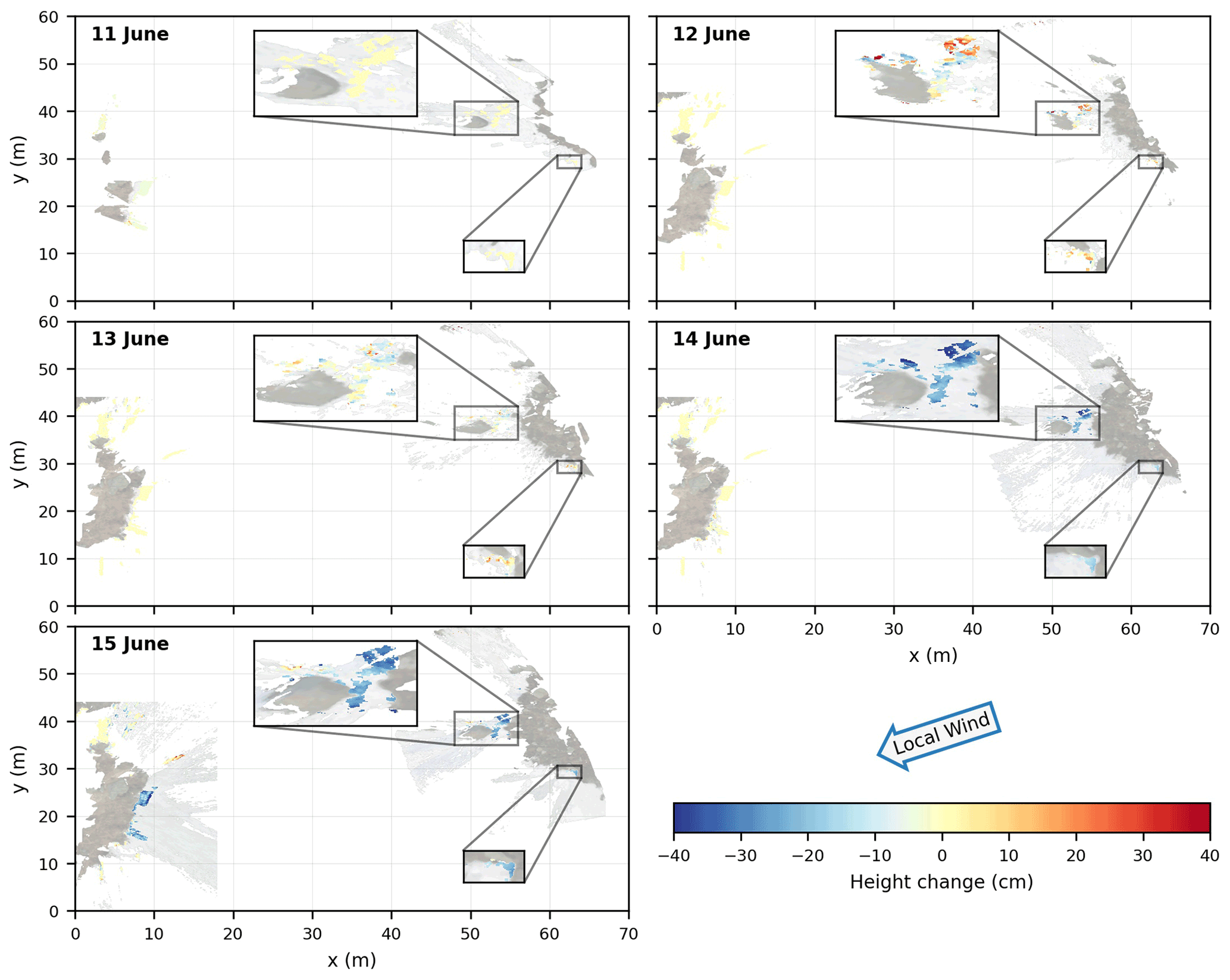
Figure A1 The resulting height change maps used for Fig. 4 plotted over the real-color orthoimages, which are used for distinguishing snow from bare ground, after removing isolated groups of cells and median filtering. The insets show zoomed areas of the upwind edge for more detail.

Appendix B: Surface generation

To create the surfaces for the simulations, noise is generated in Fourier space such that seemingly random patterns with a specified wavelength arise. These wavelengths are prescribed in the form of 2D power spectra. This method is applied so that patches at opposing walls fit together and flow that leaves the system on one side continues over the same snow patch when it reenters the system on the opposite wall. This enables the model to solve the periodic boundary conditions.

Initially, a field with random phases between 0 and 2π is generated. These phases are applied in Euler's law (i.e., $e^{i\mathit{\phi }}=\cos \mathit{\phi }+i\sin \mathit{\phi }$) such that the phases are described in exponential form. The phases are multiplied with the desired magnitude per phase such that the Fourier space is generated ($z=\left|z\right|e^{i\mathit{\phi }}$ and Figs. B1–B3). Eventually, a 2D field with dominant patterns is obtained by returning to physical space by using the inverse fast Fourier transform in Fourier space. Also, to avoid numerical instabilities in MicroHH, a Gaussian filter is applied on the surface with a standard deviation of 1 grid cell. When this filter overlaps the edges of the domain, the values at the opposing edge are applied.

The specified spectra for all generated surfaces consist of two broad peaks (Figs. B1–B3). The peak with the lowest wavenumber has the higher factor and, thus, gives the dominant structures to the snow patch distribution. The peak with the higher wavenumber (i.e., 3 times the average wavenumber of the main peak) has a lower factor, such that some smaller fluctuations occur within the larger structures, giving the patches a more realistic appearance. For the surfaces in the P30m and P60m simulations, the wavenumber of the main peak is reduced by a factor of 2 and 4, respectively, compared to the surfaces in the P15m and P15m-NB simulations. This implies an average snow patch length in reality of 15, 30, and 60 m for the P15m (and P15m-NB), P30m, and P60m simulations, respectively.

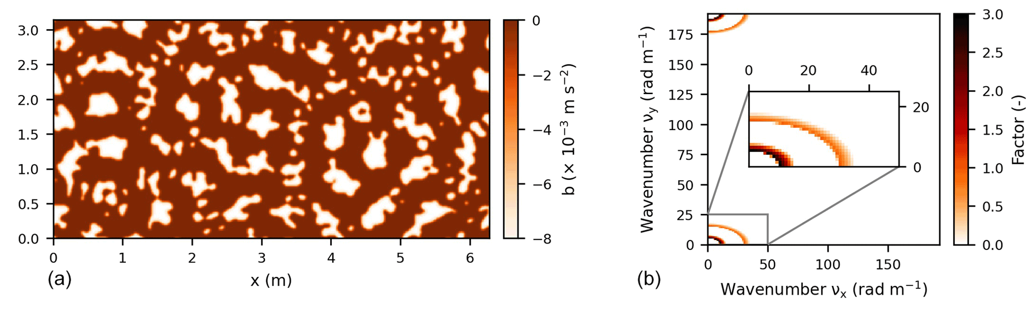
Figure B1 Generated surface temperature and the applied Fourier space in absolute form for the P15m and P15m-NB simulations. The generated surface temperature (a) was obtained by applying the inverse fast Fourier transform in Fourier space (b).

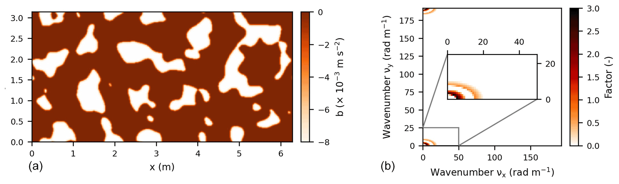
Figure B2 Generated surface temperature and the applied Fourier space in absolute form for the P30m simulation. The generated surface temperature (a) was obtained by applying the inverse fast Fourier transform in Fourier space (b).

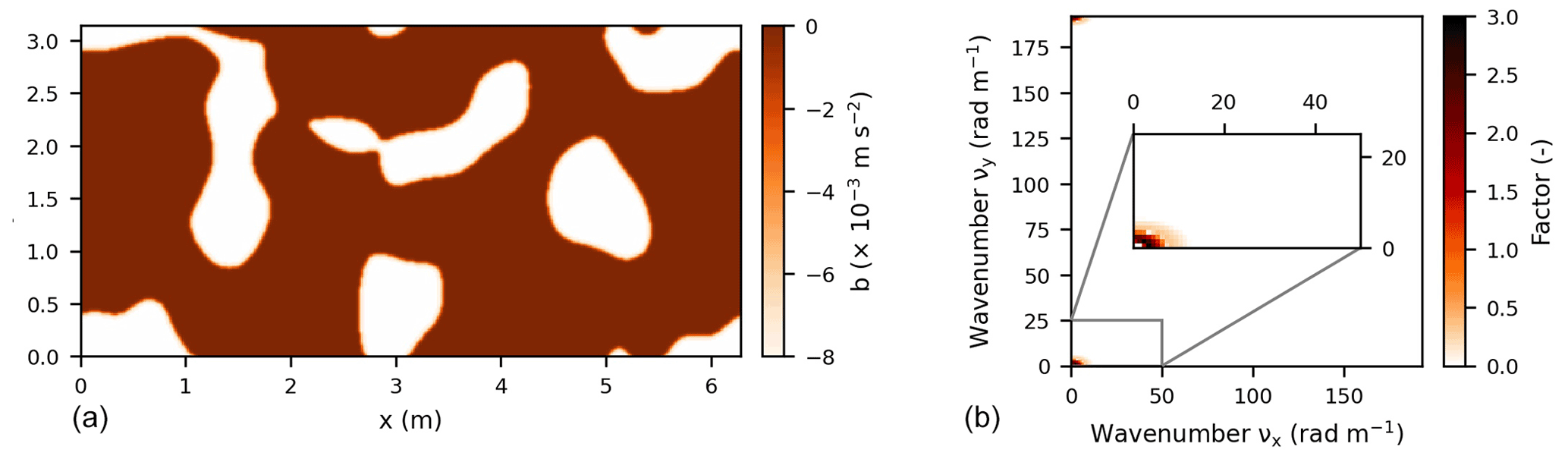
Figure B3 Generated surface temperature and the applied Fourier space in absolute form for the P60m simulation. The generated surface temperature (a) was obtained by applying the inverse fast Fourier transform in Fourier space (b).