the Creative Commons Attribution 4.0 License.
the Creative Commons Attribution 4.0 License.
 | 11 Oct 2022
Rain on snow (ROS) understudied in sea ice remote sensing: a multi-sensor analysis of ROS during MOSAiC (Multidisciplinary drifting Observatory for the Study of Arctic Climate)
Julienne Stroeve
Vishnu Nandan
Rosemary Willatt
Ruzica Dadic
Philip Rostosky
Michael Gallagher
Robbie Mallett
Andrew Barrett
Stefan Hendricks
Rasmus Tonboe
Michelle McCrystall
Mark Serreze
Linda Thielke
Gunnar Spreen
Thomas Newman
John Yackel
Robert Ricker
Michel Tsamados
Amy Macfarlane
Henna-Reetta Hannula
Martin Schneebeli
Arctic rain on snow (ROS) deposits liquid water onto existing snowpacks. Upon refreezing, this can form icy crusts at the surface or within the snowpack. By altering radar backscatter and microwave emissivity, ROS over sea ice can influence the accuracy of sea ice variables retrieved from satellite radar altimetry, scatterometers, and passive microwave radiometers. During the Arctic Ocean MOSAiC (Multidisciplinary drifting Observatory for the Study of Arctic Climate) expedition, there was an unprecedented opportunity to observe a ROS event using in situ active and passive microwave instruments similar to those deployed on satellite platforms. During liquid water accumulation in the snowpack from rain and increased melt, there was a 4-fold decrease in radar energy returned at Ku- and Ka-bands. After the snowpack refroze and ice layers formed, this decrease was followed by a 6-fold increase in returned energy. Besides altering the radar backscatter, analysis of the returned waveforms shows the waveform shape changed in response to rain and refreezing. Microwave emissivity at 19 and 89 GHz increased with increasing liquid water content and decreased as the snowpack refroze, yet subsequent ice layers altered the polarization difference. Corresponding analysis of the CryoSat-2 waveform shape and backscatter as well as AMSR2 brightness temperatures further shows that the rain and refreeze were significant enough to impact satellite returns. Our analysis provides the first detailed in situ analysis of the impacts of ROS and subsequent refreezing on both active and passive microwave observations, providing important baseline knowledge for detecting ROS over sea ice and assessing their impacts on satellite-derived sea ice variables.
- Article
(17857 KB) - Full-text XML
-
Supplement
(1259 KB) - BibTeX
- EndNote


Over the past 50 years, the Arctic has warmed 3 times faster than the planet as a whole (AMAP, 2021). While this amplified Arctic warming is most strongly manifested in autumn as a result of summer sea ice loss (e.g., Serreze et al., 2009), recent studies have also documented an increase in frequency and duration of winter warm spells that can lead to air temperatures reaching 0 ∘C near the North Pole (Graham et al., 2017). At the same time, there is evidence that Arctic rain-on-snow (ROS) events during the cold season are becoming more common (Meredith et al., 2019; Liston and Hiemstra, 2011). A recent study further suggests Arctic precipitation will increase more strongly than previously projected through 2100, with an earlier transition from snow to rain (McCrystall et al., 2021). When rain falls on snow, or when air temperatures rise above freezing, it can dramatically alter snowpack properties such as snow density, grain size, and snow water equivalent (SWE) content (Langlois et al., 2017; Grenfell and Putkonen, 2008). Upon refreezing, ice layers may form within the snowpack. On land, ROS exacerbates flooding (Li et al., 2019) and increases soil temperatures and snowmelt (Westermann et al., 2011; Putkonen and Roe, 2003; Rennert et al., 2009), while subsequent icy layers can impact wildlife, such as seal denning (Stirling and Smith, 2004), or inhibit foraging, leading to massive mortality of caribou, reindeer, and musk oxen (Putkonen et al., 2009; Forbes et al., 2016).
As a result of the ecological and societal importance of these events, several remote sensing techniques have been developed to detect ROS over land using active and passive microwave sensors. Wet snow causes backscatter to decrease, as the presence of liquid water increases the dielectric permittivity, and thus signal absorption (Kim et al., 1984; Webb et al., 2021), while refrozen ice layers lead to a strong increase in backscatter (Mortin et al., 2014). Since the backscatter difference between melt and refreeze periods is generally larger than day-to-day variations, a threshold on temporal backscatter variability can reveal when ROS has occurred (Bartsch et al., 2010). For passive microwave emissions, liquid water in the snowpack increases emissivity (Vuyovich et al., 2017). The dependence is stronger at lower frequencies because of the change in emission depth associated with melt. The response is also polarization-dependent; horizontal channels exhibit stronger responses (Anderson, 1997). Taking advantage of these emissivity dependencies, Dolant et al. (2016) developed a detection algorithm based upon vertical (V) and horizontal (H) brightness temperature gradient ratios between 19 and 37 GHz.
ROS detection over sea ice has by comparison been largely unexplored, with the only study to date based on partitioning of precipitation phase from atmospheric reanalysis (Dou et al., 2021). In that study, atmospheric reanalysis products were used to track changes in spring ROS events over sea ice, concluding that they are occurring earlier than they did 4 decades ago. However, detection of these events in winter could be important for satellite retrievals of various geophysical variables. Similar to over land surfaces, winter ROS events over sea ice can generate ice layers at the surface or within the snowpack that could modify emitted and backscattered radar energy used to retrieve various sea ice geophysical variables, such as sea ice concentration, ice thickness, snow depth, and the timing of melt onset and freeze-up. An issue particular to sea ice is that surface crusts or ice layers in the snowpack can result in an apparent vertical upward shift in the dominant scattering surface, affecting retrievals of sea ice elevation and hence sea ice thickness. While ROS events have not been specifically researched with regards to their influence on radar altimetry, Willatt et al. (2010) showed that morphological features including ice layers in snow-covered Antarctic sea ice reduced the probability that the snow–ice interface was the dominant scattering surface at Ku-band, while King et al. (2018) found that ice lenses altered ice thickness retrievals by a factor of 2 in the Arctic. Nandan et al. (2020) demonstrated a 2-fold difference in dielectric constant between snow and refrozen ice layers, leading to an elevated peak that accounted for 15 % of the total simulated Ku-band return power. Besides generating an ice layer upon refreezing, ROS further impacts the overall surface roughness of the snowpack (Seifert and Langleben, 1972). Combined, these snow property changes alter radar backscatter. Given that currently all CryoSat-2 radar-altimeter-derived sea ice thickness data products assume the dominant scattering surface is the snow–ice interface, the presence of liquid water, changes to snow structure, and/or ice layers resulting from a cold-season ROS event could bias thickness retrievals. Without accounting for this effect, derived snow depth obtained using a combination of SARAL/AltiKa (Ka-band) and CryoSat-2 (Ku-band) radar freeboards (e.g., Guerreiro et al., 2016) or CryoSat-2 radar freeboards with ICESat-2 (laser altimeter) snow freeboards (e.g., Kwok et al., 2020) would be similarly biased.
ROS events may also lead to distinct changes in microwave emissivity and backscatter that affect melt-onset timing derived from passive sensors (e.g., the Advanced Microwave Scanning Radiometer 2 – AMSR2 – on board GCOM-W1) or Ku-band scatterometers (e.g., NASA QuickSCAT – Quick Scatterometer). Furthermore, retrievals of ice concentration, ice type, snow depth, and thin ice thickness from passive microwave radiometers spanning L-band to 89 GHz may be similarly impacted. Voss et al. (2003) already demonstrated that increased surface roughness following a melt–refreeze period alters the emitted microwave energy, resulting in errors in retrieved first-year ice (FYI) and multiyear ice (MYI) fractions.
During the 2019–2020 Multidisciplinary drifting Observatory for the Study of Arctic Climate (MOSAiC) (Krumpen et al., 2020), a suite of surface-based, active and passive microwave systems was deployed to monitor the seasonal evolution of snow and ice properties, microwave backscatter, and emissivity. Sensors spanned 0.5 to 89 GHz and were deployed at the same location with overlapping footprints. Here, we present the first observations of a ROS event on sea ice observed by an in situ Ka- and Ku-band radar, together with coincident observations from a microwave radiometer at 19 and 89 GHz. By taking advantage of this unique opportunity of having several remote sensing instruments deployed at the same time, we provide key baseline knowledge for developing ROS retrieval algorithms over sea ice and understanding ROS impacts on retrieved sea ice variables such as snow depth, ice thickness, and sea ice concentration. While this event occurred 2 weeks prior to when key sea ice variables, such as ice thickness and snow depth, were retrieved, similar modifications to the snowpack during the cold season are expected if the event occurred a few weeks later. Thus, this study has relevance to winter sea ice retrievals in the face of increased frequency and intensity of ROS and/or winter warming events.
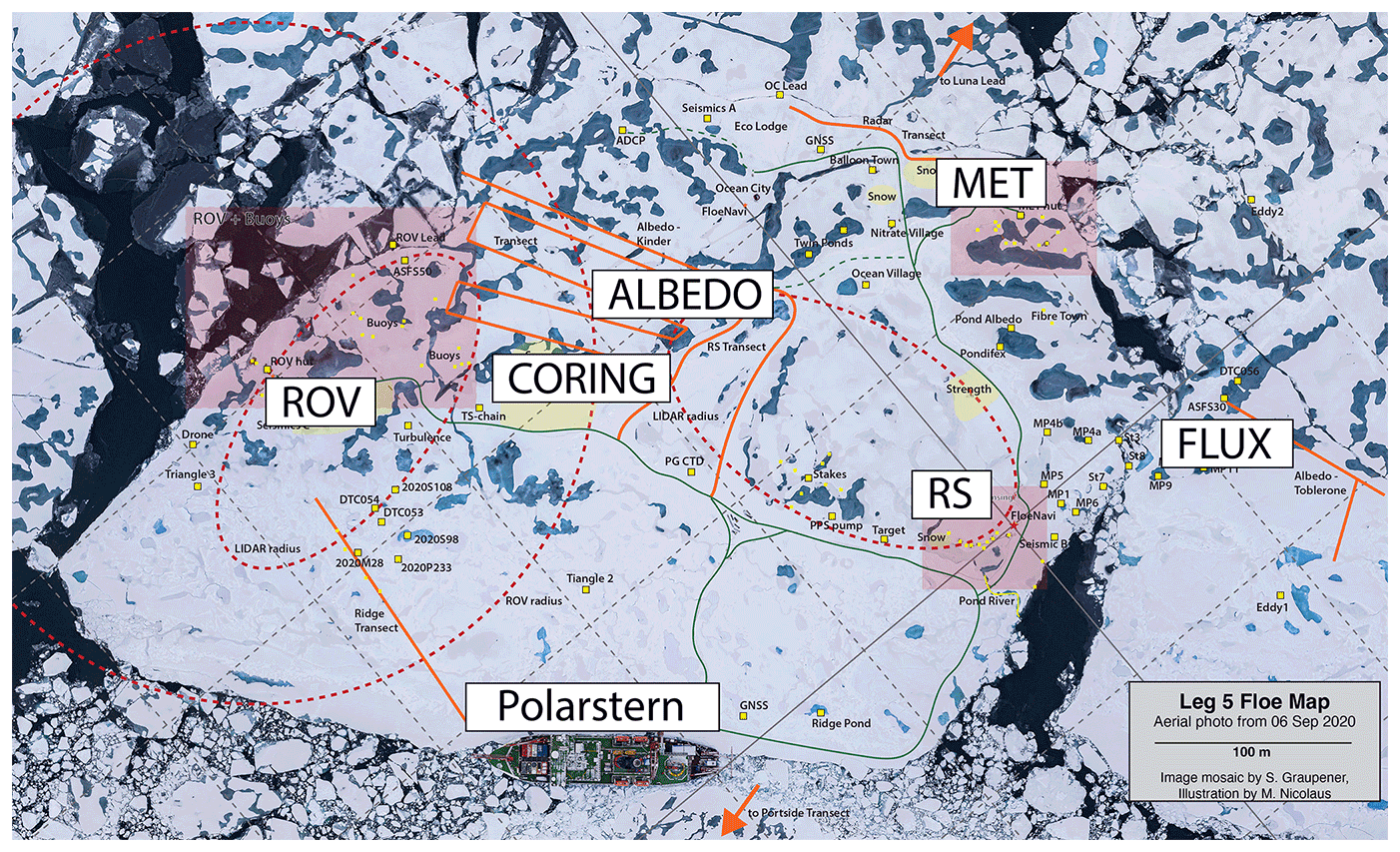
Figure 1Aerial photo showing the location of R/V Polarstern (bottom center) relative to the position of the remote sensing (RS) site (middle right of image). Also shown are the locations of MET City, where the meteorological observations used in this study were obtained (upper right of image), and the remote sensing and the albedo transects (center of image). MET City was ∼100 m from the RS site. The floe was located at roughly 89∘ N, 109∘ W. Snow pit areas are highlighted in yellow. RS and MET City as well as the ROV and buoy sites are highlighted in pink.
The radar and radiometer were deployed on a large ice floe at the dedicated MOSAiC remote sensing (RS) site. The location of the RS site relative to R/V Polarstern and MET City (where the 12 m tall meteorological tower was installed), as well as locations for the snow pit sampling during Leg 5 (21 August–20 September 2020), is shown in Fig. 1. The ice thickness near the RS site was about 1.4 m. Details of the remote sensing site setup can be found in Nicolaus et al. (2022).
2.1 Surface-based dual-frequency radar (KuKa radar)
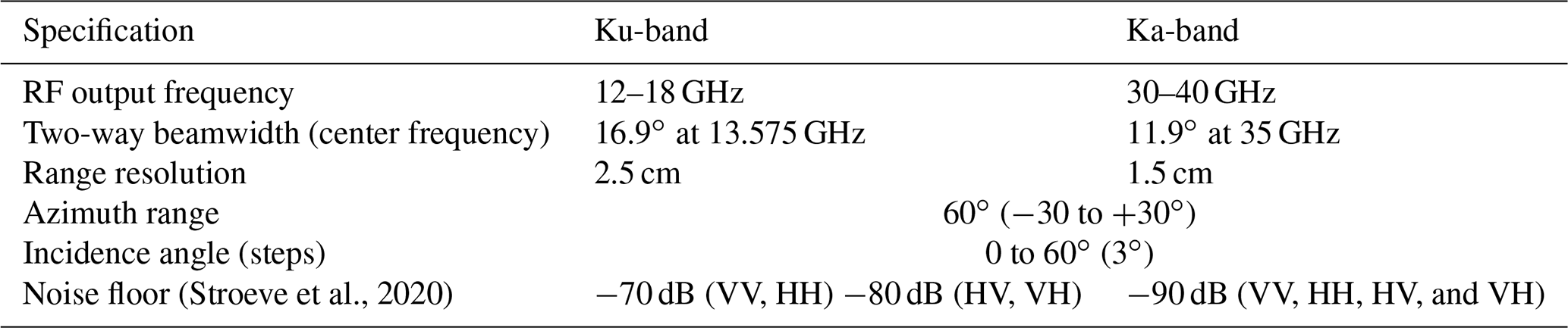
The Ka- and Ku-band surface-based radar (KuKa radar) was a newly built system by ProSensing Inc. and designed for polar deployments (see Stroeve et al., 2020). FMCW (frequency-modulated continuous-wave) radars, such as the KuKa radar, are particularly suited to applications requiring high range resolution for which the observed range interval is small and where the high processing gain allows low peak transmit powers. The KuKa radar is fully polarimetric (VV, HH, HV, and VH, where V represents vertical polarization, H is the horizontal polarization, VV and HH represent co-polarized backscatter, and HV and VH represent cross-polarized backscatter) and transmits Ku-band waves at 12–18 GHz and Ka-band waves at 30–40 GHz, with bandwidths of 6 and 10 GHz, respectively (Table 1). The KuKa radar uses separate transmit and receive antennas for both Ka- and Ku-bands that allow simultaneous transmission and reception of signals and a 100 % duty cycle. Deconvolved data are used to reduce side lobes caused by chirp non-linearity (see Appendix for details on the deconvolution).
The KuKa radar was deployed during MOSAiC Legs 1–2 and 4–5 and operated as both a scatterometer (scan mode) and an altimeter (nadir mode). In scan mode, the radar was mounted on a pedestal, scanning hourly along an azimuthal width of 60∘ (between −30 and azimuth range) and from nadir to a viewing angle (θ) of 60∘ in 3∘ increments. During nadir mode, the instrument was fixed to look at nadir and was towed along a transect. During MOSAiC, KuKa was configured to match the center frequencies of Ka-band AltiKa at 35 GHz and Ku-band CryoSat-2 at 13.575 GHz. Compared to satellite systems, KuKa has significantly higher bandwidth, providing improved range resolution of 1.5 (Ka-band) and 2.5 cm (Ku-band), compared to 30 and 46 cm for AltiKa and CryoSat-2, respectively. On 16 January 2020, an external trihedral corner reflector calibration was conducted during Leg 2 at the RS site, positioned ∼10 m in the antenna’s far-field region.
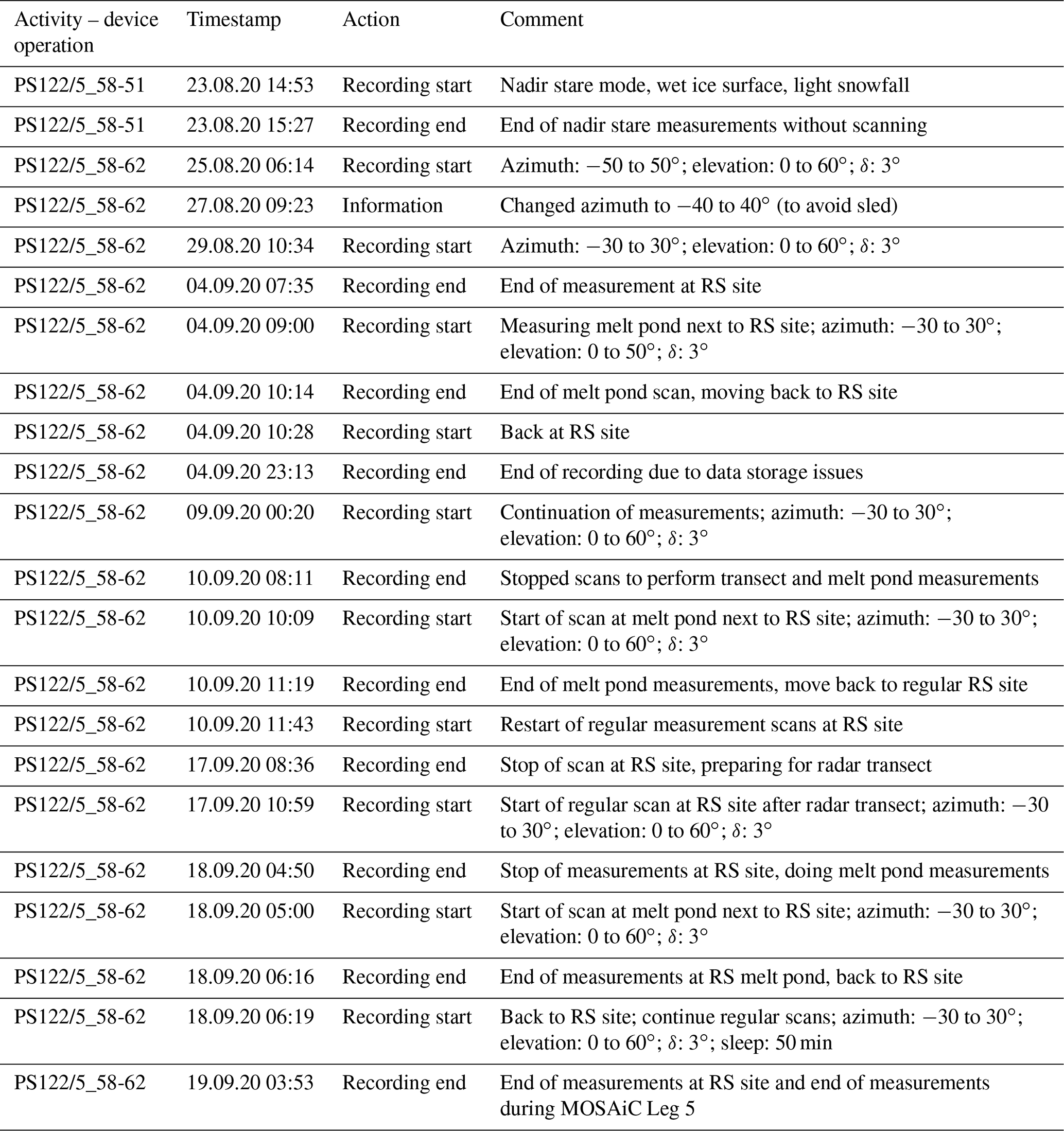
In this study, we only evaluate the data from the scan mode while the instrument was deployed at the RS site, which also includes nadir scans. Table A1 lists the measurement periods of KuKa during Leg 5. A total of 559 scans were obtained between 25 August and 19 September 2020. A data gap exists between 08:50 and 13:00 UTC on 13 September as a result of a power outage to the RS site already on 12 September, but the universal power supply (UPS) kept the KuKa radar measurements until 08:50 UTC on 13 September. We focus our analysis on the normalized radar cross-section (NRCS) values at nadir and at 45∘, mimicking θ of satellite radar altimeters and microwave scatterometers. NRCS (also termed sigma0) is given in decibels (dB) and describes the radar backscatter as a function of antenna range to the scattering particles and snow physical properties and is frequency-, polarization-, and θ-dependent.
One of our objectives is to better understand the implications of ROS on altering freeboard height retrievals and thus radar-altimeter-derived ice thickness and snow depth. Therefore, we also examine radar-return waveform changes at nadir, including the dominant scattering surfaces observed before, during, and after the ROS event. Since KuKa has a beam-limited footprint and operates at 1.5 m above the surface, as opposed to CryoSat-2 and AltiKa, which are pulse-limited footprints at ∼800 km above the surface, the geometries are different, and waveform shapes and their changes are not directly comparable. Nevertheless, changes in relative backscatter contributions from surfaces, interfaces, and volumes as well as changes in waveform shape enable inference of potential impacts on retrieved freeboards. For this study, HH-polarized data, acquired at nadir and averaged over scans from −30 to −10∘ (Ka-band) and from 0 to 30∘ (Ku-band) azimuth angles, were used. The full azimuth range was reduced in post-processing to avoid snowdrifts around the sled. See Stroeve et al. (2020) and the Appendix for more details on the KuKa radar and data processing.
Table 1Operating parameters for each of the KuKa radar's radio frequency (RF) units.
2.2 Surface-based radiometer (SBR)
A surface-based dual-polarized radiometer (SBR) built by Radiometrics Corporation collected microwave emission at 19, 37, and 89 GHz and at V and H polarizations. These radiometers contain the same frequencies and polarizations as flown on past and current satellite systems (e.g., the Special Sensor Microwave Imager – SSM/I – or AMSR2). Internal sensitivities at 19, 37, and 89 GHz are 0.04, 0.03, and 0.08 K, respectively (Radiometrics, 2004). Each antenna system has a 3 dB half-power beam width (HPBW) of 6∘ (Table 2). Polarization switches are operated at ±45 ∘ from the central position, with an isolation better than 20 dB.
Table 2System parameters of Radiometrics surface-based radiometer (SBR).

During MOSAiC, the instrument was mounted to a scanning positioner that allowed the user to scan across viewing zenith angles (θ). This positioner was attached to an 80 cm metal tube and fixed to a 30 cm high komatik sled, giving a total height above the ice of 110 cm and a field of view (FOV) at nadir of about 5.7 cm. To avoid microwave emission from the sled, the SBR scanned the surface between θ=40 and 70∘ in steps of 5∘. Sometimes the instrument was configured to only collect data at , the viewing angle of many satellite platforms. The FOV at this angle is 10.1 by 17.6 cm.
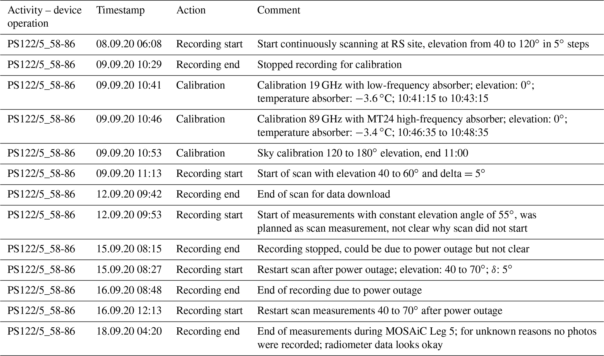
Calibrating the SBR during fieldwork operations requires two temperature blackbody target calibrations. This can be achieved by using an ambient blackbody target and a liquid nitrogen target or a sky-calibration target (e.g., pointing the instrument to an elevation of 120∘). Calibration of each 19 and 37 GHz radiometer was performed using a 0.5” thick lossy flexible foam absorber, whereas the 89 GHz channel was calibrated using a 0.5” thick microwave absorber foam. Physical temperatures were made of the absorber pads and the ambient air temperature. Comparison of the slope of the radiometer measurements to the physical measurements provides for a relative calibration of the brightness temperatures. A calibration was performed during Leg 5 on 9 September. However, for 89 GHz, results of the absorber calibration were unstable, and calibration coefficients from Leg 3 were used instead.
Output is given as brightness temperature (Tb) in kelvin (K), which is the product of the effective emissivity (ϵ) and the physical temperature (T). Table A2 lists the measurement periods of the SBR during Leg 5. As for KuKa, a power outage to the SBR instrument created a data gap between 12–13 September (the SBR did not have a UPS). In this study we only show results at as this is the most relevant viewing angle for current satellite missions. Note that the 37 GHz channel was unfortunately unstable, showing at times unphysical fluctuations of more than 50 K, and thus we only focus on results at 19 and 89 GHz.
2.3 Meteorological data and ERA5 atmospheric reanalysis
We analyze 2 m air (Tair) and skin temperatures from the 10 m high meteorological tower at MET City (Shupe et al., 2021), as well as precipitation rates derived from an on-ice OTT Pluvio pluviometer (Bartholomew, 2020) provided by the Atmospheric Radiation Measurement (ARM) program, also deployed at MET City. The Pluviometer is a sophisticated rain gauge designed to calculate precipitation rates based on accumulated mass. It measures precipitation falling on a 400 cm2 area with an accuracy given by the manufacturer of 0.1 mm min−1 but cannot distinguish between precipitation types. Size distribution of the falling particles was captured by the Parsivel (on-ice disdrometer) and vertical velocity from the Ka-band ARM zenith radar (KAZR; deployed at the bow of the ship). Further details on deployment of these instruments and their accuracy can be found in Wagner et al. (2022). While hydrometeor classification is difficult, near-surface air temperature, combined with vertical profiles of falling speed, can be used to categorize liquid-phase precipitation (Shupe et al., 2005). To correspond with scan intervals from KuKa, we produce hourly averages from the 1 s interval meteorological data.
The abovementioned meteorological data are used to interpret the surface property changes for the ROS event, yet there are many other in situ observations available beyond what is presented here. A comprehensive overview of the wide range of observations can be found in Wagner et al. (2022). Much of these data were also analyzed for this study but will not be included to remain concise. From the available data, atmospheric soundings also provide important context for the thermodynamic structure of the atmosphere and are briefly discussed but not shown. Instead, the suite of meteorological and precipitation data presented here allows for straightforward interpretation of how modification of surface properties impacted the remote sensing signatures.
To expand our study beyond the time period of this particular ROS event and to examine how wintertime ROS may be changing over time, we additionally make use of precipitation amount and type from ERA5 reanalysis (Hersbach et al., 2018). ERA5 was previously found to agree well with precipitation measurements from North Pole drifting station data (Barrett et al., 2020), as well as with snowfall timing and accumulation obtained during MOSAiC (Wagner et al., 2022). Hourly ERA5 data at resolution are used here to assess trends in cumulative, cold-season (October through April), non-frozen precipitation over the Arctic Ocean between 1980 and 2020. This is done by first identifying and removing frozen precipitation (snow and ice pellets), leaving rain, freezing rain, wet snow, and mixed rain–snow. We further remove precipitation falling at a rate <0.1 mm d−1, since ERA5 forecasts include trace precipitation most days (Barrett et al., 2020). Results are then time-averaged only where rain falls in grid cells that contain sea ice (ice concentration >50 %). Results are spatially averaged over the Arctic Ocean and the Barents Sea and individually over all regions of the Arctic Ocean that contain sea ice (see Appendix). Regional averages are computed for regions as defined by the National Snow and Ice Data Center (https://nsidc.org/data/user-resources/help-center/does-nsidc-have-tools-extract-and-geolocate-polar-stereographic#anchor-7, last access: 1 January 2022).
2.4 Snow data
Routine snow pit observations were collected at representative locations around the MOSAiC floe at least twice a week per location (see Fig. 1 for locations). Density cutters (volume =100 cm3) were used to measure snow density at 3 cm vertical resolution. Snow samples collected using the density cutter were further bagged and melted to room temperature to measure salinity (parts per thousand, ppt) using a YSI30 conductivity sensor (resolution =0.1 ppt and accuracy or ±0.1 ppt). Needle-point thermometers recorded temperature at the snow surface, at the snow–ice interface, and at 5 cm intervals in between. Snow height was measured during snow pit sampling. However, during summer and early autumn it is difficult to distinguish between the soft surface scattering layer (SSL) and snow in the field. In this study, it is the layer between snow and solid ice. Thus, the snow height and the density cutter measurements may include the SSL. Therefore, the snow height, which we discuss below, is calculated from the micro-computed tomograph (micro-CT), as the distance between the surface and the snow–SSL interface.
A micro-CT (micro-CT 45/90 computer tomography scanner from Scanco Medical AG) measured the 3-D snow structure (Hagenmuller et al., 2016). Using the snow microstructure data, snow density (ρsnow) can be derived as (Legagneux et al., 2002; Hagenmuller et al., 2016), where Vice is the ice fraction volume, Vtotal the total sample volume, and ρice=917 kg m−3 the ice density (Kerbrat et al., 2008; Hagenmuller et al., 2016). We also compute the specific surface area (SSA) as SSA = SA, where SAice is the ice surface area. Density-cutter- and micro-CT-derived bulk ρsnow are in good agreement, with differences of up to 15 % (see Fig. S1 in the Supplement). We also use the micro-CT data to derive the SWE for snow only (i.e., excluding the SSL). This was done by integrating the SWE for each micro-CT profile point, with SWE , where z= layer thickness or resolution =1.445 mm) between the snow surface (s) and the snow–SSL interface (int) (Fig. 4). The snow–SSL interface was determined visually from micro-CT images.
Figure 2 summarizes the meteorological and bulk snow properties before, during, and after the two ROS events. On 13 September, Tair rose above 0 ∘C (10:00 UTC) and mostly remained above freezing until 09:40 UTC on 14 September (Fig. 2a). Precipitation began around 05:00 UTC on 13 September and lasted 8 h (Fig. 2b), with the majority of liquid precipitation falling during this period, starting first as graupel, then turning to sleet and then to rain. The positive air temperatures lead to surface melt even before a second precipitation event started around 01:00 UTC on 14 September, characterized by rain and mist and lasted ∼3 h. Sounding observations (not shown) show that the large fall velocities observed by the KAZR (Fig. 2c) correspond to the passing of a warm air mass. Observations during the largest rain rates indicate air temperatures above zero extended to slightly above 1 km above the surface. Combining information from observations of temperature, fall velocities, precipitation rate, and particle size distributions, it is straightforward to conclude that significant liquid deposition at the surface and melt of the snowpack occurred throughout 13 September with minor liquid precipitation but continuing snowmelt early on 14 September. As surface temperatures cooled again midday on 14 September, and the soundings further indicated cooler vertical temperatures, any significant melt or liquid deposition concluded by 12:00 UTC.
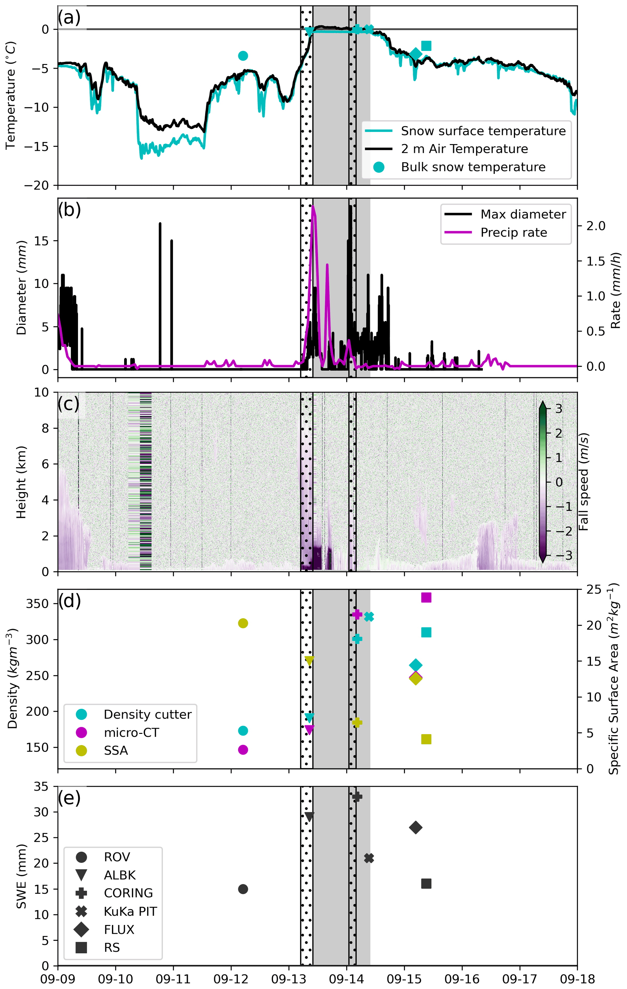
Figure 2(a) The 2 m air, skin, and bulk snow temperature; (b) precipitation rate (pluviometer) and maximum particle diameter (Parsivel); (c) KAZR mean Doppler velocity; (d) SSA and bulk snow density from both the micro-CT (snow with and without the SSL) and the density cutter; (e) SWE and snow depth. Different symbols denote the different snow pit locations. Shaded area indicates air temperatures above 0 ∘C surrounding the two ROS events (dotted areas).
ERA5, which assimilates MOSAiC balloon sounding data, is in agreement with the MET station data, showing a transition of precipitation to liquid form; precipitation began as frozen snow–ice pellets on the morning of 13 September, followed by sleet and rain between noon and 20:00 UTC, until turning to wet snow and a mixture of rain and snow on 14 September (see Fig. S2). The positive temperatures triggered melt onset in the snowpack, which also contributes to the increase in liquid water content in the snowpack. ERA5 shows that the weather system originated east of Finland and crossed Novaya Zemlya and Franz Joseph Land. Another weather system passed near the MOSAiC floe on 14 September (see animation in the Appendix).
Surface-based observations show that the snow was dry prior to rainfall. Snow had been steadily accumulating over bare ice since 3 September, without any observed melt. Accumulation 10 d preceding the ROS was a combination of snowfall, wind drift, and surface hoar deposition; the 2 d prior were characterized by widespread deposition of large surface hoar crystals (11 September) and riming (12 September; Figs. 3, 4a; ROV). Evolution of surface snow conditions between 12 and 15 September is shown in Figs. 3 and 4.
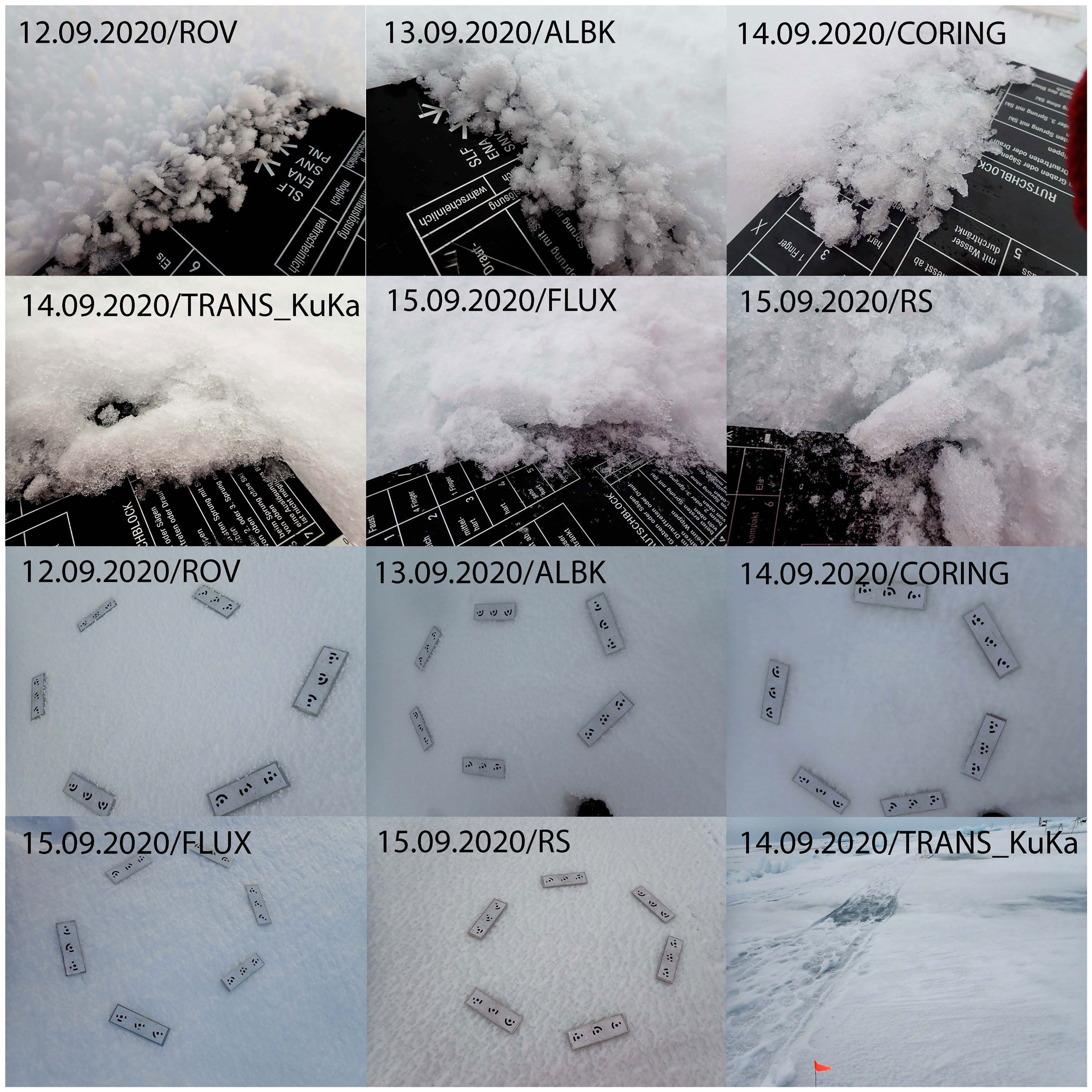
Figure 3Photographs of snow surface grain size (together with the snow grain size cards) and surface conditions (with reference targets for photogrammetry) at various locations on the MOSAiC floe during the rain-on-snow event. Locations and dates are provided on each photograph.
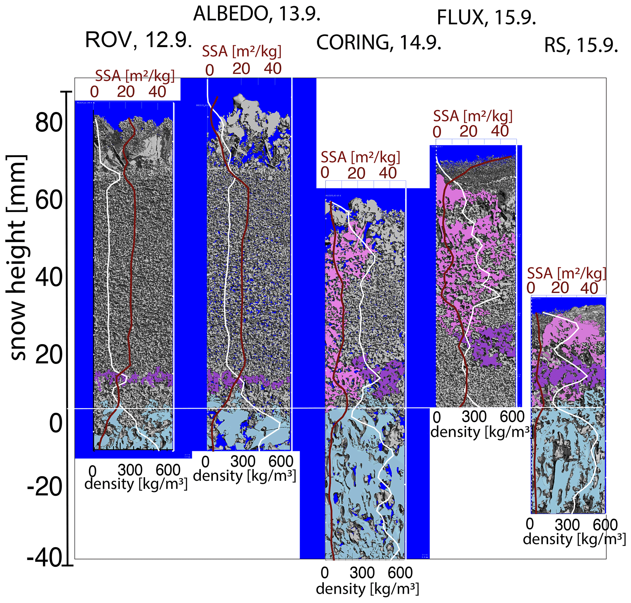
Figure 4Micro-CT images of the snowpack before, during, and after the rain on snow, together with micro-CT-derived ρsnow (white line) and SSA (dark-red line) profiles from which depth-averaged values are calculated (e.g., bulk density and SSA). The samples were taken at the following locations: ROV, ALBEDO, CORING, FLUX. To illustrate the changes in the snowpack and changes in the SSL thickness in this figure, the bottom of the snowpack is represented by 0 (horizontal white line). Above 0 is snow, and below is surface scattering layer (SSL), marked in light blue. Pink marks the water percolation paths, and purple marks the dense layer that causes water pooling after the rainfall.
Prior to rainfall, the snow height at the ROV snow pit on 12 September was 7.9 cm, and the snow plus SSL had a bulk density of 173 kg m−3 based on the density cutter (see Fig. 2d). The micro-CT-derived density and SSA profiles show relatively constant density and SSA with depth except just below the snowpack, where the surface scattering layer is present (Fig. 4). Figure 4 shows clear differences between snow and the SSL (defined as zero in Fig. 4), with the SSL having a coarser and anisotropic structure reflecting its origins from sea ice. SWE of snow only, as retrieved from the micro-CT data, is 8.9 mm. On 13 September, a snow pit was collected at the albedo site (08:30 UTC) after it had started to rain. The snow height of this pit was 8.0 cm. The micro-CT profile data show that only the top part of the snowpack was wet during the time of sampling (large drop in SSA near the surface on 13 September; Fig. 4), indicating that the rain had not yet percolated through the entire snowpack, and the snowpack had not started to melt. The bulk density slightly increased (190 kg m−3) compared to the previous day (Fig. 2d). Bulk snow temperature on 13 September was ∼0 ∘C (Fig. 2a), and the SWE of snow only increased to 11.3 mm (Fig. 2e). The larger increase in SWE measurements that include the SSL reflects SSL thickness changes due to temperature increase.
On 14 September, after the rain had percolated into the snowpack (see percolation path in pink in Fig. 4) and the melt onset, and during the second rainfall event, bulk density increased to 300 and 332 kg m−3 at the coring site and along the KuKa transect, respectively (Fig. 2d). This bulk density increase partly reflects the thicker SSL (because of increased snow–ice melt), but the density of the snow layer only is also increased to 263 kg m−3. The entire snowpack had low SSA and higher density (Fig. 4). Photographs show that the rain and additional snowmelt caused local ponding and wet slushy snow (Fig. 3; KuKa), characterized by rounding of the large grains of rimed surface hoar and compaction of the snowpack (see micro-CT image in Fig. 4c). Local ponding and smaller snow height could also explain the higher density at the KuKa transect pit. The microstructure shows that part of the measured profile was the SSL, which had increased in thickness due to warmer temperatures and melt and could therefore be sampled as part of the snowpack. The snow height decreased to 6.0 cm, while the density increased, indicating settling of wet snow and compaction of the snowpack. The SWE of the snow column increased to 15.4 mm, despite the decrease in snow height, indicating denser and wetter snow. The SWE including the SSL was 33 mm.
On 15 September, after the rainfall ended and temperatures dropped below freezing, snow pits sampled from the FLUX and RS sites show a drop in bulk temperature to −3.1 and −2.2 ∘C (Fig. 2a), respectively, yet significant differences in SWE, density, and SSA between the two snow pits (Figs. 2d, e and 4d, e). The earlier pit (FLUX site) shows surface dusting of snow (Figs. 3 and 4), resulting in much higher SSA at the surface, slightly higher SWE of snow (16.5 mm), slightly higher snow height (6.7 cm), and lower bulk density (264 kg m−3). The snow pit collected 5 h later (RS site) shows a mostly completely refrozen snowpack (2.8 cm snow height) with new snow only accumulating in small depressions, reduced SWE (7.3 mm, snow only) and SSA, and a higher snow density (277 kg m−3). This highlights potential spatial variability in snow conditions, yet it is difficult to separate spatial variability from temporal changes since the snow pits were not sampled at the same time. Considering that the snow temperatures on 15 September were below freezing, it is unlikely that such big temporal changes were possible. On the other hand, almost all profiles exhibit a higher-density layer ≈10 mm above the snow–ice interface (Fig. 4, purple layer), indicative of a possible refrozen layer. This layer is also less permeable, leading to internal ponding of percolated water, as seen in Fig. 4c and d (purple area). The snow–ice interface temperature was slightly negative (−0.5 ∘C) on 13 September, 0 ∘C on 14 September, and negative on 12 and 15 September. Salinity in the snow pits prior to 15 September was zero. On 15 September, snow salinity measurements were just above 0 ppt, but still less than 0.1 ppt, which is within the accuracy of the conductivity sensor.
Given that surface conditions were generally similar across the floe, these observations broadly represent snowpack conditions viewed by KuKa and the SBR. Next we describe the evolution of radar backscatter and microwave emission corresponding to these changes in snowpack properties.
4.1 KuKa radar
Radar backscatter remains relatively stable at both Ka- and Ku-bands prior to rainfall (Fig. 5a–b). At nadir, VV ≈ HH, indicating dominant surface scattering from the air–snow and within-snow interfaces (Onstott, 1992). At , VV backscatter is slightly greater than HH, and backscatter is dominated by volume scattering from snow grains (Tjuatja et al., 1992). The overall magnitude of the co- and cross-polarized backscatter is higher at nadir compared to , especially for Ku-band HH and VV (i.e., by ∼8 dB), also indicating strong surface scattering from the air–snow interface.
During the first ROS event, radar backscatter declines at both frequencies and all polarizations as a result of increasing signal attenuation by liquid water, due to greater dielectric loss (Ulaby and Stiles, 1980). The decline is larger at Ka-band due to stronger sensitivity of higher frequencies to snow surface changes: Ka-band backscatter reduces ∼12 (at both VV and HH) and ∼18 dB (HV) at all incidence angles. At Ku-band, VV and HH remain relatively stable at nadir but decrease by ∼7 (at both VV and HH) and by 10 dB (HV) at . Soon after the onset of melt and the second ROS event, the snowpack transitions to a funicular regime (i.e., liquid water occupies continuous pathways through the snow pore spaces; see pink areas corresponding to the water percolation paths in the micro-CT images in Fig. 4). This results in downward percolation of liquid water via gravity drainage (Colbeck, 1982a; Denoth, 1999), resulting in a completely saturated snowpack. This likely leads to the large backscatter decline during the melt onset and the second rain event. Ka-band backscatter declines by ∼12 dB, while Ku-band declines by more than 15 dB at all polarizations; the decline is larger at nadir. The steeper decline at nadir from the first ROS event suggests stronger signal attenuation likely from the ponded and slushy snow surface directly in front of the radar, possibly due to rainwater dripping from the KuKa antenna horns, though this cannot be confirmed. Overall, Ka- and Ku-band backscatter during the ROS event fell 4 and 6 standard deviations (16.5 and 19.3 dB), respectively, outside the observed backscatter variability before the ROS event.
After the snowpack refreezes, HH and VV nadir backscatter increases approximately 20 and 25 dB at Ka- and Ku-bands, respectively, and remains slightly higher than before the ROS (see pre- and post-kernel density plots). This indicates an electromagnetically smoother air–snow interface due to surface refreezing, resulting in stronger surface scattering, leading to a relatively greater nadir backscatter than observed prior to rainfall. At 45∘, the difference in Ku-band VV and HH backscatter increases slightly by up to 1.5 dB, compared to nadir, and the angular dependence for Ku-band HV almost vanishes. This indicates a combination of dominant Ku-band surface scattering from the air–snow interface and some additional scattering from dense layers slightly below the refrozen snow surface. In contrast, the angular dependence gradually reduces for Ka-band VV and HH, suggesting dominant surface scattering from the increasingly colder and refrozen snow surface.
Next, we consider the impact of the ROS event on radar waveforms (Fig. 6), i.e., the shape of the power–time plot at various times before, during, and after the ROS events. Figure 6a and b show the HH-polarized power as a function of time at both Ka- (a) and Ku-band (b) as a function of range from the antennas (m). Properties such as interface roughness and dielectric contrast, as well as the frequency of the radiation, will influence how much power is detected from each location within the snow and ice. For returned power to be detected, the radiation must both penetrate through overlying layers and be scattered back in the direction of the receiver. The waveforms are therefore useful to determine where radiation penetrates to and is scattered from to understand the waveform shapes (distribution of power vs. range) and interpretation of backscatter values. Arrows indicate locations of the selected waveforms shown in the inset to the right of the echograms. As discussed in Stroeve et al. (2020), the range from which most power is returned corresponds to the air–snow interface in both Ka- and Ku-bands. As we saw with the backscatter changes, the waveforms are stable before the first ROS event (e.g., black sample, 13 September, 00:25 UTC), and power is returned from the air–snow interface and also from below. During the rainfall event (dark-green sample, 13 September, 08:49 UTC) the power from the air–snow interface has reduced, but the echo shape is otherwise similar.
Following the first rainfall period (magenta waveforms, 13 September, 13:58 UTC), most of the power is returned from the air–snow interface, and the power returned from ranges greater than ∼1.6 m drops in both bands, causing a shadow-like region of lower power in the echograms. Note also the shift in the peak return in the green samples relative to the black ones in the inset towards shorter range at Ka-band. During the second ROS event (cyan and brown waveforms on 14 September, 01:10 and 02:06 UTC), the peak power associated with the air–snow interface decreases, and there is a further shift to shorter ranges, now also evident at Ku-band.
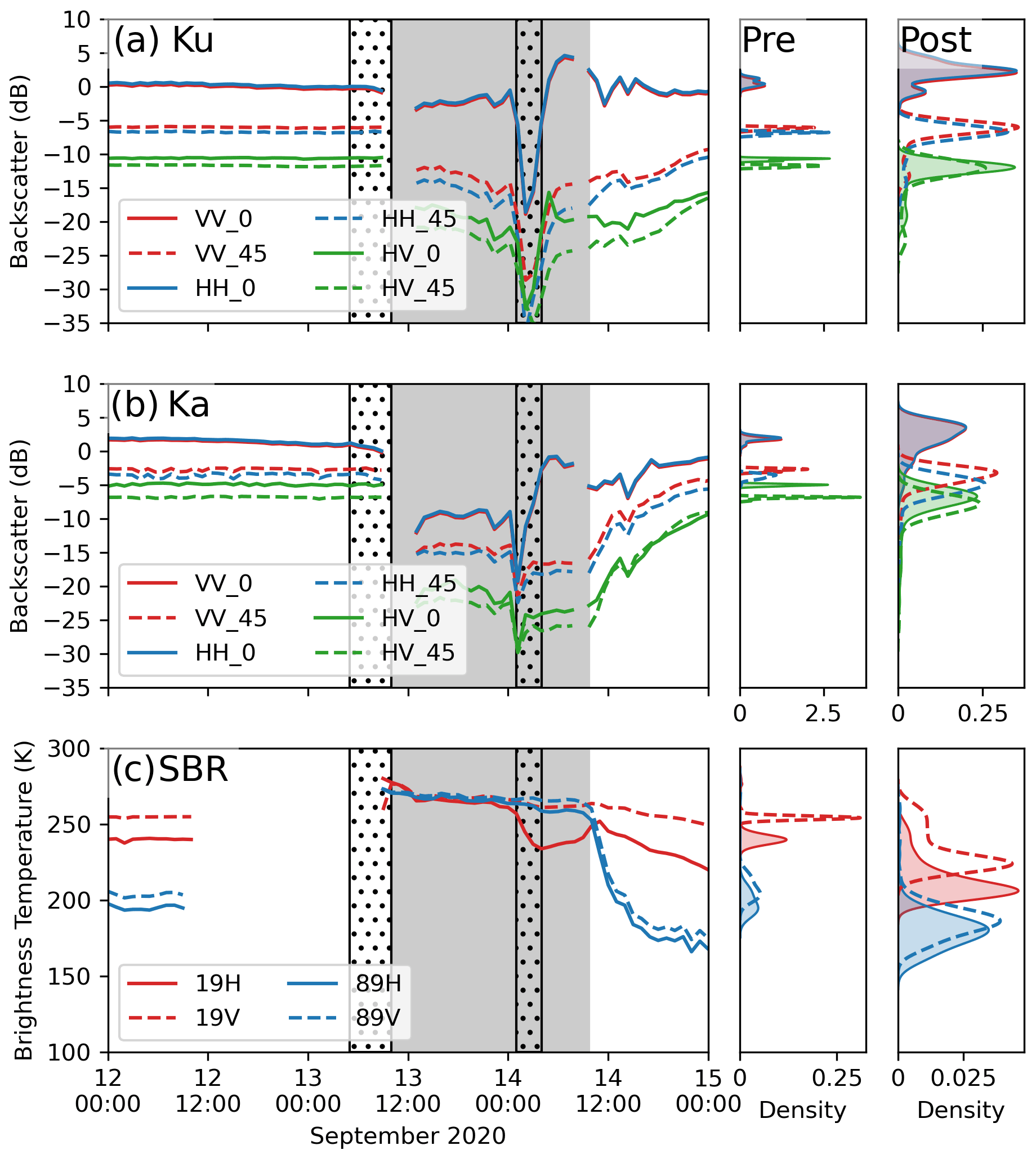
Figure 5(a) Ku- and (b) Ka-band radar backscatter measured at nadir and , (c) 19 and 89 GHz brightness temperatures at horizontal and vertical polarizations at . Corresponding kernel density distributions are shown in the right panels before and after the ROS event. Shaded and dotted areas are the same as in Fig. 2. Note the difference of 1 order of magnitude in the kernel density distributions between pre- and post-ROS event.
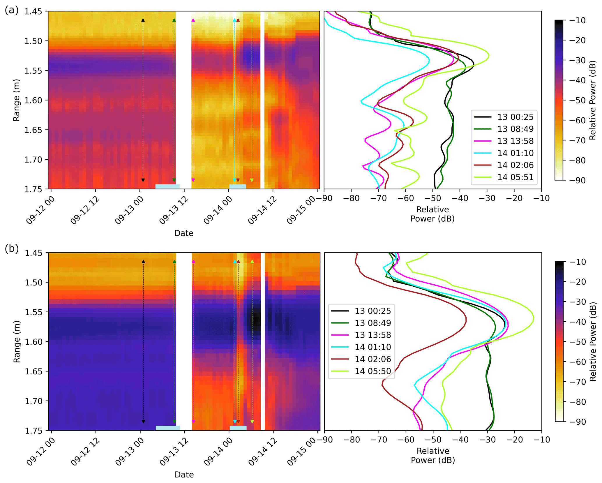
Figure 6(a) Ka- and (b) Ku-band HH echograms at nadir, indicating scattering from different ranges, hence waveform shape over time. Vertical white stripes indicate data gaps. Light-blue boxes at the base indicate the rainfall periods. Inset panels on the right indicate waveforms selected at the dates and times shown by the arrows in the echograms, demonstrating changes in waveform shape, and leading edges during the 24 h period.
Following this, the refrozen snow surface increases scattering from the air–snow interface (lime waveforms, 14 September, 05:50 UTC). The small shift in the range to the peak could be caused by scattering from higher in the snowpack, from the instrument sinking into the snow, or from some combination; we cannot determine which, and we therefore do not draw conclusions based on this observation. The radar was moved once again on 14 September at 08:24 to scan a different area, then replaced back to scan the study area again from 14 September 09:42. After this it appears that more power is once again returned from below the air–snow interface, presumably as the temperature drops from 14 September at UTC, and the remaining water in the snowpack freezes into ice. This would reduce absorption of the radiation at the air–snow interface, allowing it to penetrate further into the snowpack.
The change in waveform shape from the black to the lime waveforms demonstrates that after the two rain events, a greater proportion of the returned power is associated with a peak at the air–snow interface, and a smaller proportion is associated with ranges below the peak. During the ROS event the waveform peak power was reduced, and these data also suggest that after a ROS event, changes to the snow structure affect its scattering properties and hence waveform shape. Considering the contributions to the waveforms, where returned power is detected by KuKa, this indicates that the radiation could penetrate to that level and that it was scattered from it.
To see how these results are applicable at satellite scales, we investigated the change in CryoSat-2 waveforms during this time period, using AWI (Alfred Wegener Institute) CryoSat-2 L1P data. We plot the peakiness, which is an indicator of waveform shape related to the ratio of maximum to mean power, and sigma0 (Fig. 7). As shown, during the two ROS events between 13–14 September, there are changes to the waveform peakiness near the MOSAiC floe much greater than elsewhere in region shown. Since the CryoSat-2 peakiness increases, this suggests that more of the power is returned from a smaller number of range bins as the peak power increases relative to the mean along the waveform. CryoSat-2 sigma0 also changes, increasing on 13 September before reducing over the next few days, but it does not return to the level (16–17 dB) prior to the ROS events.
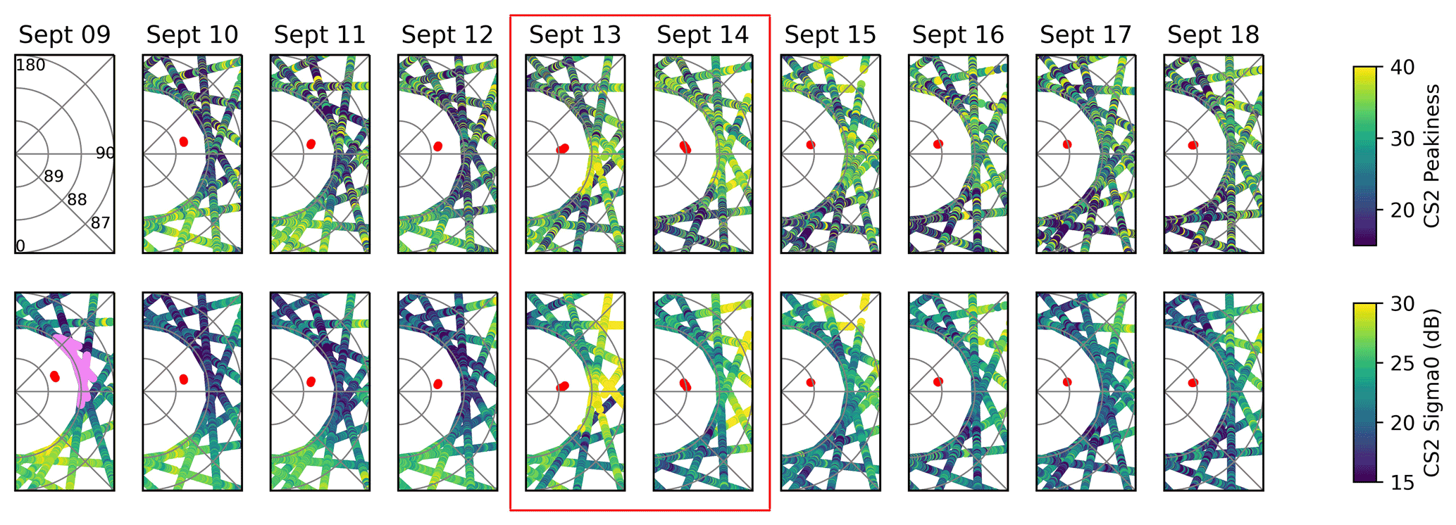
Figure 7CryoSat-2 peakiness (top) and sigma0 (bottom) before, during, and after the ROS events on 13 to 14 September (red box). Only waveforms with peakiness less than 40 are shown, as this is the cutoff for classification as a sea ice floe within the ice pack (waveforms with peakiness greater than 40 are classified as originating from leads.) Red circles indicate the locations at which KuKa collected data on that date. Lines of latitude and longitude are indicated in the top right panel, and the lilac points in the bottom left panel show CryoSat-2 data points within 130 km of KuKa, from which the averaged quantities shown in Fig. 8 are determined.
These results indicate that the ROS altered the CryoSat-2 waveforms, consistent with what we see in the KuKa data. Time series of (waveform) peakiness and sigma0 of CryoSat-2 and KuKa Ku-band (to match CryoSat-2) waveforms are overlaid in Fig. 8. KuKa Ku-band peakiness is computed by taking the subset of range bins above the noise floor (−70 dB) and dividing the maximum power of any of those bins by the mean power averaged across all of them to calculate a peakiness value for each time interval using a similar methodology to CryoSat-2. The CryoSat-2 data are averaged over a 130 km circle radius centered at KuKa's location each day; 130 km was selected to only include CryoSat-2 data collected as close as possible to KuKa whilst ensuring that at least two CryoSat-2 tracks were within the radius for each date. Due to the locations of the tracks, points were included from CryoSat-2 tracks in the afternoon and evening each day (ranging from 16:41–23:17 UTC), whereas KuKa data were gathered at hourly intervals.

Figure 8Time series of peakiness (a) and sigma0 (b) for CryoSat-2 (red squares) and KuKa Ku-band data (blue circles) averaged over 24 h periods. The blue sections indicate periods of rain.
The top panel shows that waveform peakiness changed in a similar way for KuKa Ku-band and CryoSat-2: increasing sharply in response to rainfall and subsequent refreezing, then reducing, yet staying higher than before the ROS. Note that this can also be seen in the KuKa Ka-band data in Fig. 6a, where the brown echo (following refreezing) is peakier than the black echo (prior to ROS events). The bottom panel indicates that sigma0 also changes in both KuKa Ku-band and CryoSat-2 waveforms, but not in the same way; KuKa sigma0 reduces around the ROS events, then increases following subsequent refreezing, whilst CryoSat-2 sigma0 increases following the ROS events, then reduces over time. Yet again note that sigma0 remains higher than before the ROS also in the CS2 data. Unlike peakiness, which is likely to vary in a similar way between the instruments, sigma0 is likely to be highly spatially variable, and this may be one reason that the sigma0 calculated from the two instruments does not vary in the same way. Also, as noted above, due to the CryoSat-2 orbit, the data within 130 km of KuKa were gathered during the afternoon and evening each day, and the ROS events took some time to pass over the CryoSat-2 tracks and KuKa locations; hence the effects would differ in terms of the timing of changes to sigma0. Lastly, CryoSat-2 has a synthetic aperture radar (SAR)- and pulse-limited footprint of 300×1500 m compared to the 45 cm beam-limited footprint of the KuKa Ku-band instrument; CryoSat-2 footprints will include ridges and smooth and rough snow and ice surfaces, whilst KuKa was surveying one flat area; hence the sigma0 backscatter may vary differently depending on what is included in the footprint and how it is affected by the precipitation.
4.2 Surface-based radiometer (SBR)
The bottom panel of Fig. 5 shows the corresponding time series of brightness temperature Tb at 19 and 89 GHz during the ROS event together with the kernel densities before and after the ROS event. Prior to rain, Tb is relatively stable. Brightness temperatures at 89 GHz are lower than at 19 GHz because volume scattering in the snow is larger at 89 GHz. The overall mean and standard deviation of the Tb prior to rainfall are K, K, K, and K. These observations are within the range reported by Harasyn et al. (2020) over first-year sea ice in Hudson Bay observed in June for dry snowpacks, as well as those recorded by satellite over Arctic first-year and multiyear sea ice (see Appendix in Ivanova et al., 2015). On the morning of 13 September, the Tb increases sharply to nearly 274 K at both frequencies in response to liquid water in the snowpack. The increase to 274 K gives an indication of the absolute calibration of the radiometer (it should not increase above 273.15 K). It also reflects the fact that emissivity of a wet snowpack is nearly 1 because of high absorption, and the physical snowpack temperature at the top is slightly above 0 ∘C. This also suggests that at the time the data were collected, the entire snowpack was wet since the 19 and 89 GHz channels are equally impacted, and thus the emission originates from the top of the wet snowpack at both frequencies.
Midday on 14 September, Tb drops to cold conditions again, immediately impacting 89 GHz as the top of the snowpack refreezes. The 19 GHz channels, with deeper penetration depth, take longer to respond as the rest of the snowpack takes longer to refreeze or dry out completely from drainage. After the event, the snowpack remains cold, yet it is altered. In particular, the 19 GHz polarization difference (PD) (i.e., PD ) is larger than before the ROS event, increasing from 14 to 17 K after the entire snowpack is refrozen (e.g., between 16 and 18 September). This increase is likely the result of ice layers in the snowpack (e.g., high-density layers shown in Fig. 4e); the 89 GHz PD on the other hand decreases from 9.4 to 6.1 K. Further, grain size increased throughout the snowpack, and thus Tb is lower than before it rained (more volume scattering), affecting both 19 and 89 GHz, which decreased to 206±4.2 (19H) and 224±2.3 GHz (19V) as well as 181±9.4 (89H) and 187±8.02 GHz (89V). The larger standard deviation at 89 GHz is likely because this frequency is particularly affected by snow grain and structure scattering. Further, the 89 GHz channel is also impacted by atmospheric downwelling radiation, and small temperature fluctuations at the snow surface will influence penetration, leading to temporal fluctuations in Tb.
We further investigated if this particular ROS event is captured in satellite passive microwave observations. AMSR2 is able to detect this rain event (Fig. 9); AMSR2 Tb sharply increases at all frequencies during the ROS, most strongly at 89 GHz (increase of ∼35 K). This is consistent with the larger increase at higher frequencies observed in the SBR. Similarly, the initial decline afterward is stronger at higher frequencies because they are more sensitive to changes in the top layers of the snowpack, and it takes time for the entire snowpack to refreeze. The polarization difference increases for the lower-frequency channels after the snowpack refreezes, with the largest polarization change at 18.7 GHz, in line with the SBR observations at 19 GHz. The agreement in response to the ROS event and subsequent refreezing between AMSR2 and SBR is remarkable given the large spatial- and temporal-resolution differences in the two measurements and further illustrates that the ROS covered quite a large region.
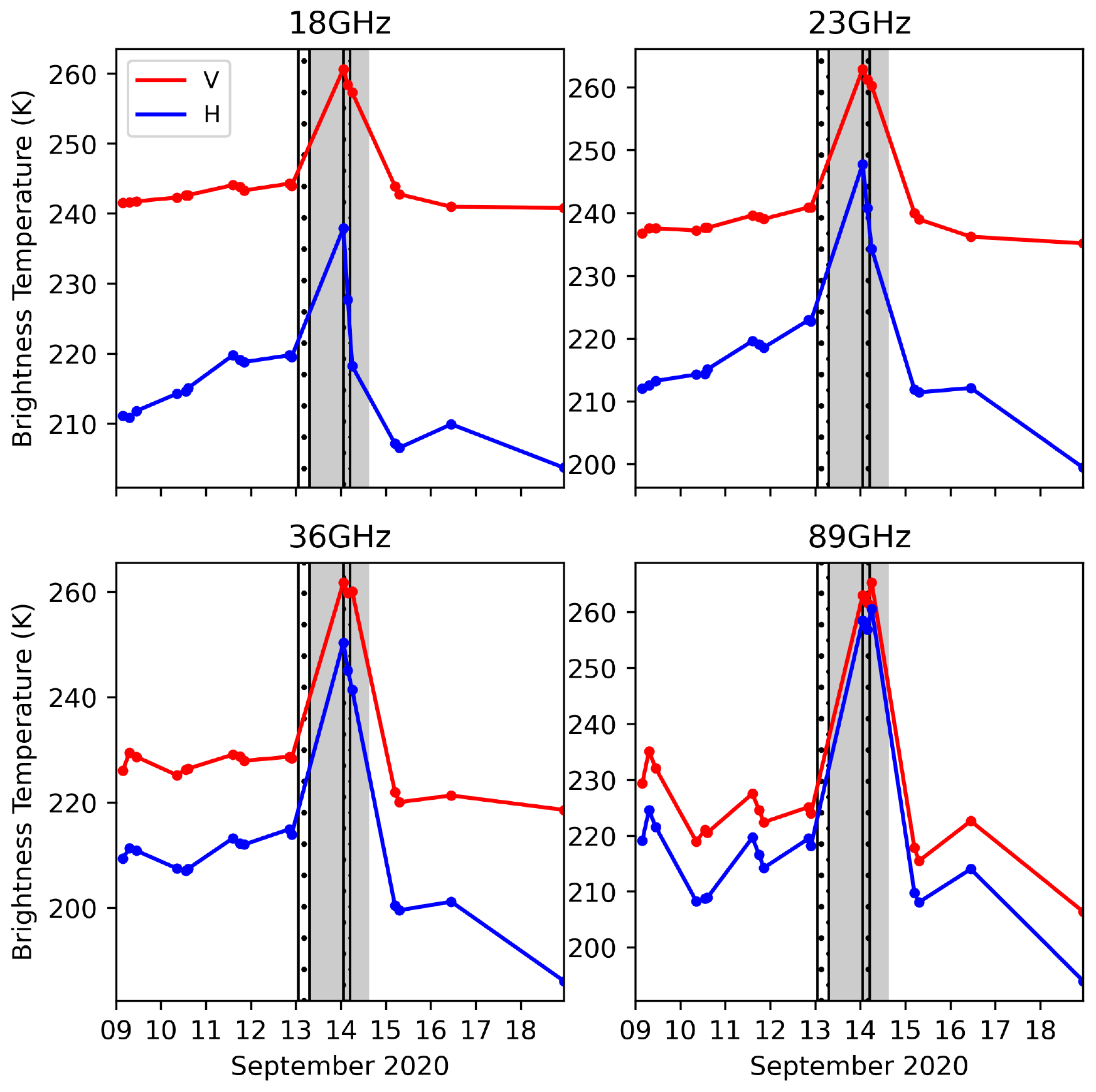
Figure 9AMSR2 brightness temperatures from 9 until 18 September. Data are shown for the MOSAiC floe location as extracted from individual swaths (see Table A3).
5.1 Radar altimetry
Radar freeboard height retrievals are based on assumptions as to where the dominant scattering horizon is located, i.e., the snow–ice interface at Ku-band and air–snow interface at Ka-band (e.g., Tonboe et al., 2021). Our waveform analysis suggests that the peak associated with the dominant scattering surface moved upwards (to a smaller range) after the second ROS event and refreezing. The shift is 0.9 (Ka-band) and 1.5 cm (Ku-band). This could be due to rainwater refreezing at the surface, raising its elevation, and/or decreasing roughness at nadir. Another contribution could be settling of the radar; it is not possible to verify whether the sled sank into the melting snow, and therefore we cannot quantify whether this partially or fully accounted for the apparent change in range.
Instead we focus on changes in the waveform shape. While satellite radar altimeters cannot resolve the peaks visible in the KuKa data, and there are important differences in range resolution and the echo shapes between KuKa and satellite radar altimeters, the in situ shape changes at both Ku- and Ka-band demonstrate that satellite-retrieved sea ice freeboards from both CryoSat-2 and AltiKa could be shifted upwards. However, satellite radar return waveforms also depend on the large-scale floe topographic variability (i.e., ridges, rubble fields), which controls the total number of illuminated point scatterers as a function of delay time. While there are challenges in upscaling to satellite footprints, KuKa data combined with measurements of physical snow characteristics could, in future studies, allow us to investigate how the combination of snow depth, temperature, salinity, and radar-scale roughness controls sigma0 and how these facet-scale factors affect the shape return pulse, as a function of transmitted pulse bandwidth. These insights can then be combined with numerical radar simulation approaches that focus on large-scale floe topographic variability (e.g., Landy et al., 2020), with realistic gain patterns, to understand how the different factors combine to influence the radar return power over kilometer-scale satellite footprints.
The change in waveform shape may further impact classification of sea ice vs. leads; lead waveforms can be distinguished from ice floes using waveform “peakiness” (Laxon, 1994), with specular returns from leads causing peakier waveforms than diffuse returns from ice floes (Peacock and Laxon, 2004). When melt ponds form, peakiness increases as the echoes become more specular (Tilling et al., 2018). The change in waveform shape caused by the ROS events affects the peakiness of the KuKa Ku-band echoes, and similar effects are seen on the CryoSat-2 echoes in that area. This indicates that ROS could affect lead and sea ice discrimination by altering the classification of a floe to a lead, artificially increasing the apparent local sea surface height and incorrectly removing a waveform from the floe dataset. Since conventional thickness retrieval methods from radar altimetry are limited to the cold season months, we cannot fully evaluate the impacts of our detected waveform shape changes on altimetry-derived sea ice thickness. In a follow-on study we will investigate the effect of our observed waveform shape changes on retrieved sea ice freeboard and thickness during the cold season.
Another consideration is the influence of ROS on the hydrostatic balance of the ice floe. In particular, by adding rainwater to an existing snow cover, its density and also its SWE is increased, which can reduce the freeboard by weighing down the floe, hence reducing the elevation of the air–snow and snow–ice interfaces above the waterline. In addition, compaction of formerly dry snow by rainwater and wet snow metamorphism, as implied in Fig. 4 (between 13 and 14 September), also reduces the snow freeboard. ERA5 indicates that an additional 11.5 mm of SWE was deposited onto the snowpack, which would depress the snow–ice interface by around the same amount (∼11.5 mm) due to Archimedes' principle. Snow density changes as a result of rainfall further impact retrieved elevations by altering the speed of radiation propagation through the snow cover (e.g., Mallett et al., 2020; Willatt et al., 2010).
Finally, it is worth noting that on FYI, ROS impacts can be even more complicated. Snow on FYI is saline (Geldsetzer et al., 2009), and the brine content alters the dominant backscatter horizon (Nandan et al., 2017). ROS can flush brine from the snow, thereby freshening the snowpack (Nandan et al., 2020). We hypothesize that, upon refreezing, a reduced brine volume and colder snowpack allow greater penetration of radar signal. Thus, the error introduced by snow salinity is reduced. In addition, the changes to snow structure and porosity may also affect the radar backscatter, and these effects may interact in complex ways.
5.2 Scatterometry
Figure 5 shows a strong reduction in KuKa radar backscatter when there is liquid water in the snowpack and an increase in backscatter as the snowpack refreezes – visible in both frequencies and incidence angles and all polarizations. Since the change in backscatter during rainfall is large compared to normal day-to-day backscatter variability, this information can be used to detect ROS events from spaceborne scatterometry and SARs and differentiate between ROS-induced melt and naturally occurring melt-onset events that presently depend on time series threshold techniques to determine the timing of spring and summer melt onset (e.g., Mortin et al., 2012).
The effects of ROS on scattering after the snowpack has refrozen could also be significant. Over FYI, if an ice layer forms right above the sea ice, it would constrain upward brine wicking through the snowpack. Formation of ice lenses within the snowpack and/or air-filled vertical ice channels, inclusions, or poly-aggregate snow grain clusters of various sizes (Colbeck, 1982b; Denoth, 1999) may also occur. While ice lenses facilitate additional surface scattering, vertically oriented ice channels produce more volume scattering, especially at large incidence angles. A more extreme impact could be complete melting of the snow cover from the rainfall, leaving bare ice, resulting in ice surface scattering.
Overall, ROS and subsequent refreezing can create geophysical and thermodynamic changes to the snowpack at various spatial scales, leading to complexly layered snowpacks, with changes in salinity- and temperature-dependent brine volume (for FYI) (Nandan et al., 2020), density (Denoth, 1999), and snow grain microstructure (Colbeck, 1982a), all altering surface and volume scattering contributions to the total backscatter. These modifications will in turn affect the reliability of SAR and scatterometer algorithms to accurately retrieve snow and sea ice geophysical properties, classify FYI and MYI types (Nghiem et al., 1995), and detect the timing of melt onset. Our results highlight that modifications during and following ROS events and their effect on microwave scattering at these frequencies are not trivial. Overall, our results provide a detailed and first-hand understanding of the geophysical impacts of ROS and its effect on the radar scattering behavior. These findings will help us to further aid interpretation of radar backscatter changes due to ROS events at satellite-scales.
5.3 Passive microwave
Finally, SIC, melt-onset and freeze-up timing, snow–ice interface temperature, thin ice thickness, and snow depth are all regularly retrieved using current satellite passive microwave systems operating at frequencies studied here (e.g., Comiso et al., 1997; Markus and Cavalieri, 2009; Markus et al., 2009; Tietsche et al., 2018; Kaleschke et al., 2016; Rostosky et al., 2018). Since the penetration into the snow–ice depends strongly on frequency, with lower frequencies penetrating further, ice layers in the snowpack will have a larger impact on retrievals relying on low-frequency channels. This includes thin ice thickness retrieved from satellites such as the Soil Moisture and Ocean Salinity (SMOS) L-band (1.4 GHz) mission, snow–ice interface temperature retrievals using 6.9 GHz from AMSR2, and snow depth retrieved using a combination of 19 and 37 GHz or 7 and 19 GHz channels.

Figure 10(a) Collocated AMSR2 and SBR polarization difference (PD) at 89 GHz (top) and (b) sea ice concentration derived from the polarization difference at 89 GHz using the ASI algorithm (Spreen et al., 2008). In addition, the sea ice concentration from the NASA Team algorithm (Cavalieri et al., 1999) is shown. (c) Gradient ratio (at vertical polarization) derived from AMSR2 37 and 19 GHz (blue) and 19 and 7 GHz (red) observations and (d) snow depth derived from GR19 7 and GR37 19 during the ROS event.
Nevertheless, impacts occur also at higher frequencies. SIC retrieved with the ARTIST Sea Ice (ASI) algorithm (Spreen et al., 2008) is based on 89 GHz polarization difference (PD), with low PD representative of high SIC values. Wet snow has an emissivity close to 1 at both V and H polarization (compared to emissivities less than 1 and different for V and H for dry snow; e.g., Eppler et al., 1992), and thus the PD decreases during ROS (Fig. 10a). In computing the ASI SIC during this particular ROS event, we modified the retrieval curve for PD differences <11.7 (tie point for 100 % SIC), since due to its polynomial dependency, the ASI algorithm saturates at SIC =100 %. To deal with saturation, we compute the SIC using the slope and intercept of the ASI retrieval equation between PD =14 and PD =11 (i.e., the SIC =80 % to SIC =100 % region) and then apply a linear fit for PD values less than 11.7. With this modification, the SIC changes observed here are representative of areas with SIC between 80 % and 100 %. This leads to a SIC overestimation of 5 % (AMSR2) to 10 % (SBR) (Fig. 10b). However, because the ASI SIC was already at 100 % at the MOSAiC ice floe, and thus limited to the maximum value, this increase cannot be seen in the operational satellite record. But if the ROS event happened in a lower SIC region, the event would have caused an overestimation, e.g., 90 % instead of 82 %.
On the other hand, the NASA Team algorithm (Cavalieri et al., 1997) relies on 19 GHz H/V polarization ratio (PR19) and 37 and 19 GHz gradient ratio (GR37 19). Both the PR19 and GR37 19 increase during the ROS event (GR37 19 shown in Fig. 10c), yielding a SIC decrease from 90 % to 70 % during ROS (Fig. 10b). The response lasts long after refreeze, as the polarization and gradient ratios are altered, leading to continued underestimation of SIC of about 10 % compared to the values prior to the rain event. The increase in the GR37 19 to 0 would additionally lead to the second-year ice floe mapped as 100 % FYI using the NASA Team algorithm. Furthermore, the decrease in GR37 19 to more negative values after the ROS event would result in an increase in the MYI fraction and in the snow depth retrieved using the Markus and Cavalieri algorithm.
Snow depth retrievals using algorithms to derive snow depth over FYI (Markus and Cavalieri, 1998; Comiso et al., 2003) and over both FYI and MYI in spring (Rostosky et al., 2018) are also impacted. While the event during September is too early in the season for a quantitative satellite snow depth retrieval, both the AMSR2 GR37 19 and GR19 7 GHz were increased during the ROS event (Fig. 10c) because of the reduced penetration depth in the snow and similar scattering at the two frequencies. If the Markus and Cavalieri (1998) snow depth retrieval method is applied (valid only for FYI), this would lead to a retrieved snow depth of 0 cm (using GR37 19), or a reduction of 50 % if using Rostosky et al. (2018) (using GR19 7), respectively (Fig. 10d). Note that the retrieved snow depth is substantially higher than the snow depth measured on the MOSAiC flow. Both algorithms are not designed to retrieve snow depth during the refreezing season. Sea ice that survived one summer melt is interpreted as deep snow by the algorithms, and thus snow depth is overestimated.
While MOSAiC offered the opportunity for a detailed in situ analysis of a ROS event, this event occurred at the end of the summer melt season, at a time before sea ice variables, such as ice thickness and snow depth, are retrieved from satellites. However, if events like rain on snow or more generally warm air intrusions happen in winter, they would likely have similar impacts on the snow cover, with liquid water percolating through the snow and refreezing. A key difference with presumably thicker snowpacks and colder snow and snow–ice interfaces in winter could be that ROS or warm air intrusions may affect a smaller vertical portion of the snow cover. Specifically, percolation into the snow might not be as deep, which once refrozen, would lead to larger biases in ice thickness retrieved from radar altimetry than during the case study shown in this paper. The question then is whether or not ROS or winter warming events are becoming more common. Some studies have already looked at increased frequency and duration of winter warming events using atmospheric reanalysis data (e.g., Graham et al., 2017). Here we examine ERA5 reanalysis to see if there is a similar increase in winter rainfall.
While there is considerable year-to-year variability, a statistically significant positive trend (at 95 % confidence interval) towards more rainfall during the winter season (October through April) is seen for the Arctic Ocean and its marginal seas (Fig. 11a). This is dominated by statistically significant trends as averaged over the central Arctic and the Laptev Sea (Figs. 11b and A4). Trends are less steep for the December-to-February period (not shown), reflecting a larger increase in wet precipitation during autumn freeze-up and melt-onset periods (e.g., October–November and March–April). While the amount of rainfall is still relatively small in magnitude, we may expect winter rainfall events to become increasingly important as the Arctic continues to warm under atmospheric greenhouse gas forcing and starts to transition to more rainfall earlier than previously predicted (e.g., McCrystall et al., 2021).

Figure 11(a) Mean wet precipitation (rain, freezing rain, wet snow, and mixed rain–snow; mm d−1) over sea ice for the cold season (October–April). Values are given as averages over the central Arctic Ocean and its peripheral seas, including the Barents Sea. The trend is determined by a two-tailed test for non-zero correlation in values over time, with a p value of 0.043. (b) Spatial trends in rainfall from 1979 to 2020 averaged from October through April.
During the MOSAiC expedition, several remote sensing instruments were deployed to better understand how snowpack and sea ice properties impact satellite retrievals of various sea ice variables. The instruments spanned frequencies relevant to both current and future (e.g., Copernicus CRISTAL and CIMR) satellite systems. A rain-on-snow event towards the end of the year-long MOSAiC expedition in September 2020 provided a unique opportunity to utilize these assets to study the impact of ROS on active and passive microwave radiation, providing information germane to developing ROS detection over sea ice and for understanding ROS impacts on derived snow depth, sea ice thickness, and ice concentration.
Notably, while the geometries of ground-based systems are different from satellite altimeters, we show that ROS can alter waveform shape, with impacts on discrimination of sea ice from leads and the potential to alter the retrieved surface elevation over sea ice and hence thickness retrievals from CryoSat-2/AltiKa. Permanent changes observed in microwave emissivity have the potential to impact retrieved ice concentrations and snow depths.
Since Fram Strait to the North Pole is often visited by temporary winter warming events (e.g., Graham et al., 2017), we may expect that this region of the Arctic is already more vulnerable to potential biases in satellite-retrieved sea ice variables as a result of ice layers from warmer air temperatures and/or rain-on-snow events. Looking forward, as the Arctic continues to warm, it is reasonable to expect an increase in the frequency and possibly intensity of ROS and winter warming events. Coupled with shallower snowpacks atop the ice cover, due to later ice formation (Stroeve et al., 2020) and the fact that snowpacks atop first-year ice have a non-negligible brine content that also affects microwave emission and backscatter (e.g., Nandan et al., 2017), thickness and snow depth retrievals will become more challenging in the coming decades, raising the importance of improving our process-level understanding and obtaining ground truth such as that collected during MOSAiC.
A1 KuKa radar instrument description
As discussed in the main body of the paper, the KuKa radar was built by ProSensing Inc. specifically for the MOSAiC expedition. In the design phase it was decided to use a frequency-modulated continuous-wave (FMCW) radar, in order to maximize the range resolution for which the observed range interval is small and where the high processing gain allows low peak transmit powers. The principles of FMCW radar operation have been outlined in a number of publications (Luck, 1949; Griffiths, 1990; Stove, 1992; Meta, 2007; Cooper et al., 2011).
FMCW radar systems typically utilize a constant-amplitude sinusoidal waveform that has been linearly frequency-modulated in time, also known as a chirp. The KuKa radar transmits Ku-band waves at 12–18 GHz and Ka-band waves at 30–40 GHz, with bandwidths of 6 and 10 GHz for the Ku- and Ka-bands, respectively. The KuKa system uses separate transmit and receive antennas for both Ka- and Ku-bands that allow simultaneous transmission and reception of signals and a 100 % duty cycle. The chirp signal is digitally generated, amplified, and then transmitted into the field of view by a transmit horn antenna. The instantaneous transmit frequency, ft, is given by , where fc is the carrier frequency, t is time, PRI is the pulse repetition interval, and B is the transmitted bandwidth, which (similar to a pulsed radar) determines the radar range resolution. Deconvolved data are used to reduce side lobes caused by chirp non-linearity (see Sect. A1.4).
The reflected echoes originating from objects within the antenna beam are collected by the receive horn antenna and then amplified by a low-noise amplifier (LNA). For the case of a single object, the received echo signal will be a replica of the transmitted waveform but delayed by time t, due to two-way propagation , where R is the object range, and c is the free-space propagation velocity (the speed of light). After exiting the LNA, the received signal is first mixed with the transmitted signal generating the intermediate-frequency (or beat) signal and then low-pass-filtered.
The advantage of FMCW radars is that they allow much lower sampling rates (compared to pulsed radars) as the sampling rate need only correspond to twice the maximum beat frequency (real signal obeying Nyquist criterion) of the farthest object within the field of view. The KuKa system has a 14 bit ADC (analog-to-digital converter) with a sample rate of 20 MHz, but the range window of interest means that this sampling rate can be reduced (after further low-pass-filtering) by a decimation factor of 16 or 32 for Ka- and Ku-bands, respectively, before digitization. The digitized beat frequency signals are then converted from their raw binary format into voltages with the signals from the different bands and polarizations and reference signals assigned to separate arrays (i.e., VV; HV; VH; HH; calibration loop signal, cal; noise).
The system is configured to operate in both fine mode or coarse mode. The default setting is fine mode, operating at a bandwidth of 6 and 10 GHz at Ku- and Ka-bands, respectively. However, the full bandwidth can be processed within any segment to achieve any desired range resolution above 2.5 (Ku-band) or 1.5 cm (Ka-band). In the coarse mode, the range resolution processing is centered on satellite frequencies of CryoSat-2 and AltiKa at 13.575 and 35.7 GHz, respectively, with an operating bandwidth of 500 MHz, yielding 30 cm range resolution. The KuKa radar was designed to be operated in a scanning mode, to simulate a scatterometer, and also in nadir mode to simulate an altimeter. In the scanning mode, the instrument was mounted on a pedestal that was fixed to a sled and deployed at each of the RS sites during Legs 1, 2, 4, and 5, with an idle time of 30 min (Leg 1) and an hour (Legs 2, 4, and 5) between the scans. Scans were made between −30 and azimuth range and between nadir and 60∘, at 5∘ increments. On 16 January 2020, an external trihedral corner reflector calibration was conducted during Leg 2 at the RS site, positioned ∼10 m in the antenna's far-field region. The software has an automatic calibration routine that scans the scene to find the peak corner reflector signal. The height of the reflector is not the same as the height of the antenna. As long as the corner reflector is pointing in the general direction of the antennas, within ±15∘, the radar cross-section of the reflector is close to the theoretical value. Table S1 in the Supplement lists the measurement periods of KuKa during Leg 5. A total of 559 scans were obtained on Leg 5 between 25 August and 19 September 2020.
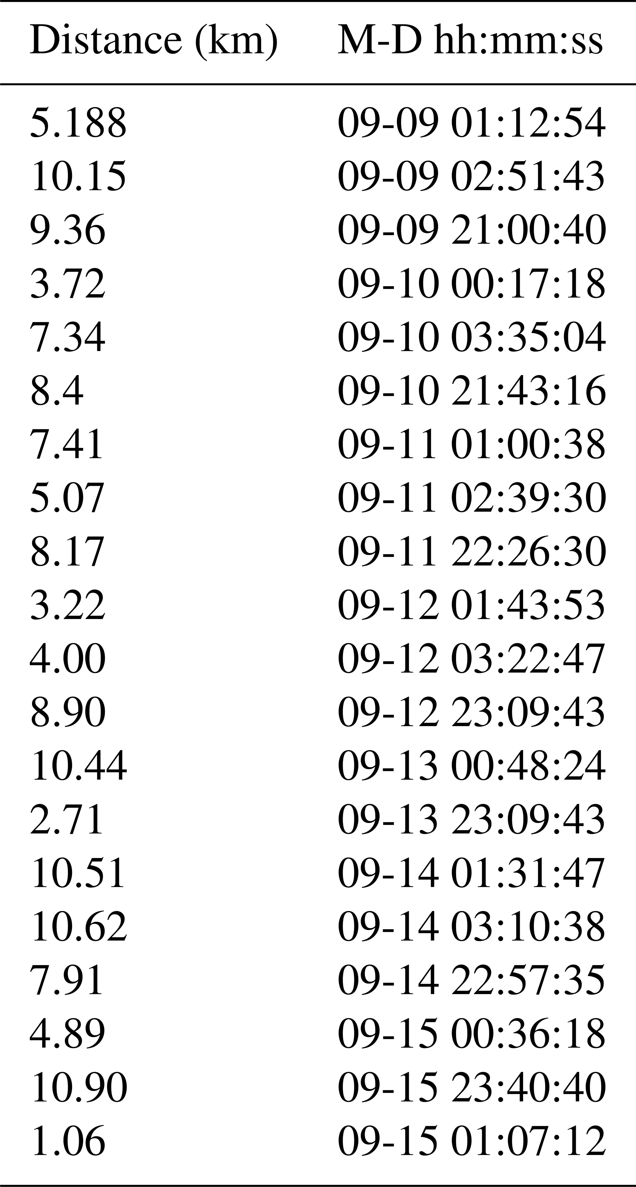
Table A1List of measurement periods for the KuKa radar during Leg 5.
A1.1 KuKa radar geometry
The antennas of each radar are dual-polarized scalar horns with a beamwidth of 16.5∘ (Ku-band) and 11.9∘ (Ka-band). The center-to-center spacings between the radar horns are 13.36 (Ku-band) and 7.65 cm (Ka-band). The horn spacing and difference in beamwidths means slightly different scanning footprint by the radar system by ∼60 % (Ka-band) and ∼70 % (Ku-band), with every 5∘ increment in incidence angle θ.
Given the ∼1.6 m height between the Ka- and Ku-band antennas above the snow surface, the radial distance, and range from the pedestal, the footprint diameter and area increase from nadir to 50∘ incidence angle. Considering the 11.9∘ (Ka-band) and 16.9∘ (Ku-band) antenna beamwidth, the KuKa radar footprint on the snow is dependent on both frequency and incidence angle. This also means the incidence angle dependence on Ka- and Ku-band footprint overlaps for a given radar “shot”. Since the incremental separation between successive incidence angles is 5∘, scans sample completely independent snow, every third azimuthal scan in the Ku-band, and every other scan in the Ka-band. The instrument footprint at nadir is 0.25 (Ka-band) and 0.4 m2 (Ku-band), and at it is 0.75 (Ka-band) and 2.25 m2 (Ku-band). In total, 3308 h scans were acquired during the year-long campaign. Table S1 summarizes the operating parameters for each Ku- and Ka-band radars.
Table A2List of measurement periods of the surface-based radiometer (SBR) during Leg 5. Note that no data were recorded between 12 September 10:38:53 and 13 September 09:54:10.
A1.2 Ku- and Ka-band NRCS measurement
The KuKa radar records a data series of six signal states: the four transmit polarization combinations (VV, HH, HV, and VH), together with a calibration loop signal (cal) and a noise signal (noise). Each data block with these six signals is then processed separately into range profiles of the complex received voltage, for each frequency through fast Fourier transform. The range profiles for each combination of polarization are power-averaged across the azimuth range, for each incidence angle.
We used the KuKaPy Python package to convert the Ku- and Ka-band raw data into calibrated polarimetric backscatter (VV, HH, and HV). Within every incidence angle scan line averaged at 60∘, Ka- and Ku-band VV, HH, HV, and VH backscatter coefficients were derived from the second-order complex covariance matrix, assuming scattering from a surface ellipse, as defined by the antenna beamwidths. From the azimuth range-averaged power profiles, the NRCS was calculated following the beam-limited radar range equation by Sarabandi et al. (1990), given by
where h is the height of the antenna; Rc is the range to the corner reflector; dB is the antenna half-power beamwidth (one-way); and and are the power recorded from the footprint and corner reflector, respectively. We discard VH based on reciprocity observed in the cross-polarized channels (i.e., HV = VH).
Uncertainties in NRCS can be attributed to polarimetric calibration error (multiplicative bias) from the metal tripod supporting the trihedral corner reflector, utilization of a finite signal-to-noise ratio (SNR), random error, standard deviation in estimated radar return power, and approximation error arising from sensor and target geometry assumptions (Stroeve et al., 2020). A detailed description of error analysis, along with a detailed explanation of radar signal processing, calibration process, and NRCS calculation, can be found in Stroeve et al. (2020).
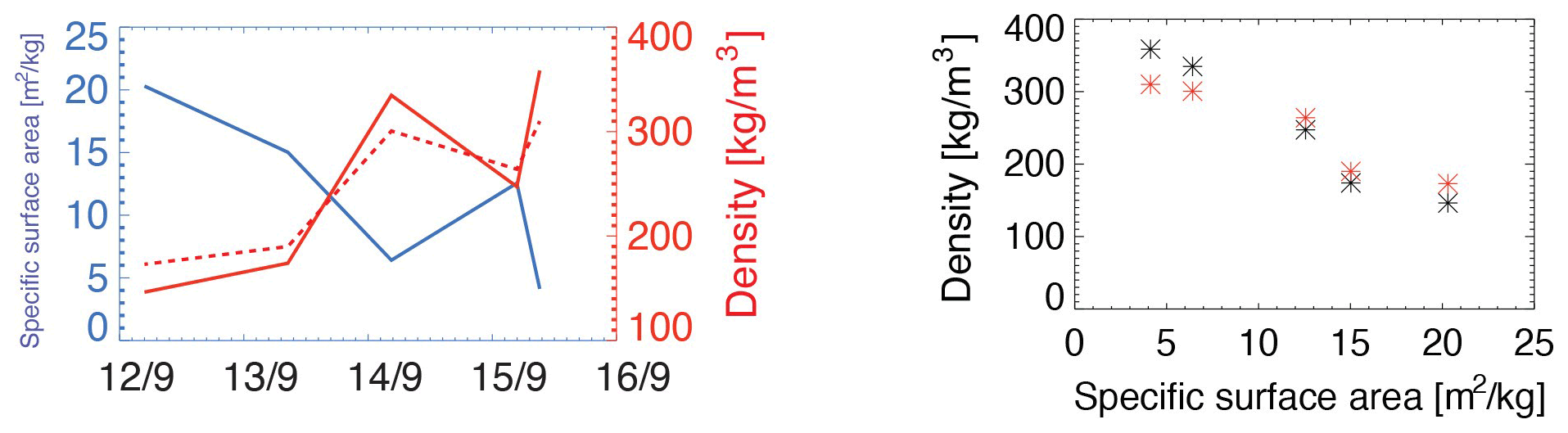
Figure A1Depth-averaged micro-CT density and specific surface area (SSA) during the rain-on-snow event and comparison with density cutter. Image on left shows the average density (red line) and SSA (blue line) from micro-CT and density cutter (dotted line). Image on the right shows the SSA vs. density from micro-CT (black) and the density cutter (red).
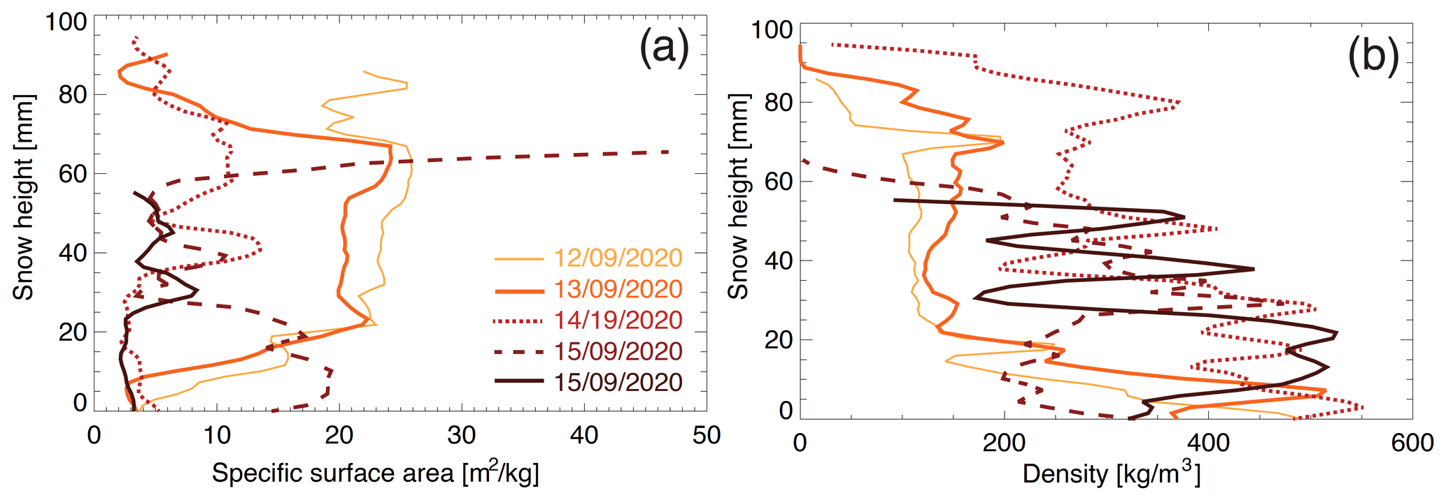
Figure A2Profiles of specific surface area (SSA) (a) and density (b) before, during, and after the rain-on-snow event. The bottom of the sample is represented by 0. Please note that the bottom of the sample is not necessarily the snow–ice interface, as discussed in Fig. 4 in the main paper.
Table A3Distance from the MOSAiC floe (km) and time of the AMSR2 swath data used in Figs. 9 and 10.
A1.3 Ku- and Ka-band waveform analysis
For a single object, the sampled beat signal will have a frequency proportional to the range to object, and if there are multiple objects within the field of view, the beat signal will consist of a linear superposition of multiple sinusoids with frequencies representing the echoes from different ranges. The mixing procedure in FMCW radars is equivalent to matched filter processing (pulse compression) used in pulsed radar systems, but with the difference that the point target response of a FMCW radar (after mixing) exists in the frequency domain rather than the time domain (as is the case for pulsed radars). To extract the frequency content of the received signals and to create range profiles of power vs. range, a Fourier transform needs to be taken of the beat signal, with the range to different objects within the field of view obtained from their corresponding beat frequencies, fb, following the expression , where T is the chirp period.
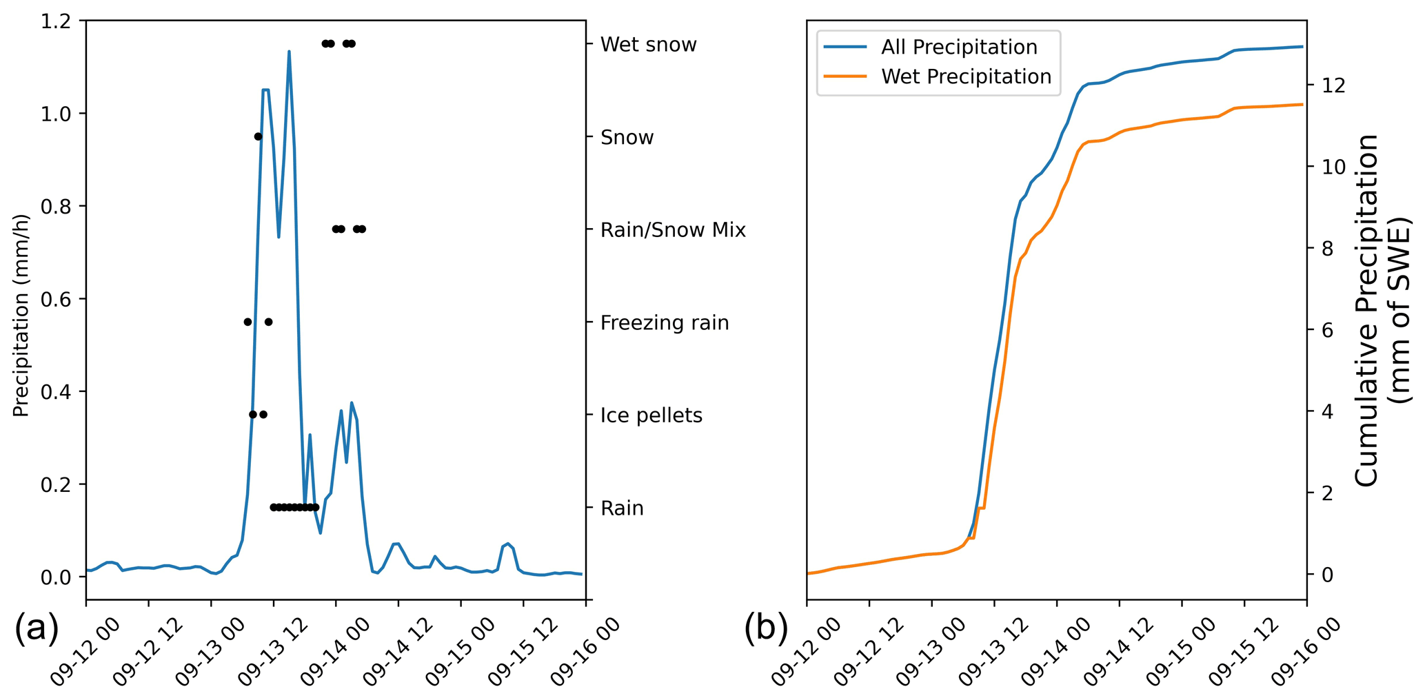
Figure A3Rain on snow from ERA5 data. (a) Time series of cumulative precipitation at the MOSAiC floe (nearest 1∘ grid cell) separated into all precipitation and wet precipitation, where the latter corresponds to all World Meteorological Organization precipitation types that are not snow or ice-pellets. (b) Time series of precipitation and precipitation type as in (a).
For the KuKa system, to obtain range profiles of relative power vs. range, each column of the separate voltage data arrays is first windowed using a Hanning window and then zero-padded. A column-wise fast Fourier transform is taken, after which these data are multiplied by a conversion factor: transforming the data into an uncorrected power spectrum. To correct for KuKa instrument drift, a correction factor is derived by comparing the values in the calibration data array with those collected under laboratory test conditions. In the next step, this uncorrected power spectrum is squared; the magnitude extracted; and the drift correction applied, forming a corrected power spectrum array. The data used in this ranging analysis consist of these corrected power spectrum arrays (one for each polarization), where each of the array columns is a range profile of relative power that has a range bin spacing of 0.46 cm for Ka-band and 0.76 cm for Ku-band. All these data are stored in the NetCDF files output by the KuKaPy programs.
For this study HH polarization data, gathered with KuKa looking at 0∘ incidence angle (nadir) and averaged over scans from −30 to (Ka) and 0 to 30∘ (Ku) azimuth angles, were used. The full azimuth range was reduced in post-processing to avoid snowdrifts around the sled. Deconvolution was applied (see below) as set in the configuration files which control the KuKaPy processing; the information from these files is copied into the resultant NetCDF files for information as needed. The output NetCDF files contain the “HH_power” and “range” variables that were used to examine how the waveform shape changed before, after, and during the ROS events.
A1.4 Deconvolution
For FMCW radars, phase and amplitude errors on the transmitted chirp can degrade radar system performance and introduce range side lobes (Griffiths, 1990; Budge and Burt, 1993; Piper, 1995; Ayhan et al., 2016). This paper uses standard techniques to correct for both amplitude and phase non-linearities to mitigate against the side lobes (Vossiek et al., 1996; Zhaodu et al., 1996; Meta et al., 2006; Dengler et al., 2007). Sweep non-linearities are characterized from electrically smooth lead surface returns (collected on 23–24 January 2020) and compared with a unity-amplitude ideal linear sweep. Non-linearities are corrected by applying the processing flow outlined in (Frischen et al., 2015) with an additional step that utilizes high-pass-filtering to mitigate the effect of the transmit or receive leakage signal (Stove, 1992). As deconvolution waveforms from January 2020 were the only available option, and the radar response changes with time, the deconvolution is not optimal. Nevertheless, it provides some side lobe reduction.
A2 Surface-based radiometer (SBR) instrument
Microwave emission of the snow and sea ice surface was measured using the University of Manitoba surface-based radiometer (SBR), which consists of three dual-polarized (vertical and horizontal) radiometers (19, 37, and 89 GHz) together with a GPS to record location and date and time. A camera is also housed in the system to capture images of the surface in the approximate field of view (FOV) of the radiometers. Each radiometer contains a 16 bit analog-to-digital converter and is equipped with a Texas Instruments MSC1211 microcontroller. As discussed in the Radiometrics user manual, internal sensitivities are 0.04 (19 GHz), 0.03 (37 GHz), and 0.08 K (89 GHz).
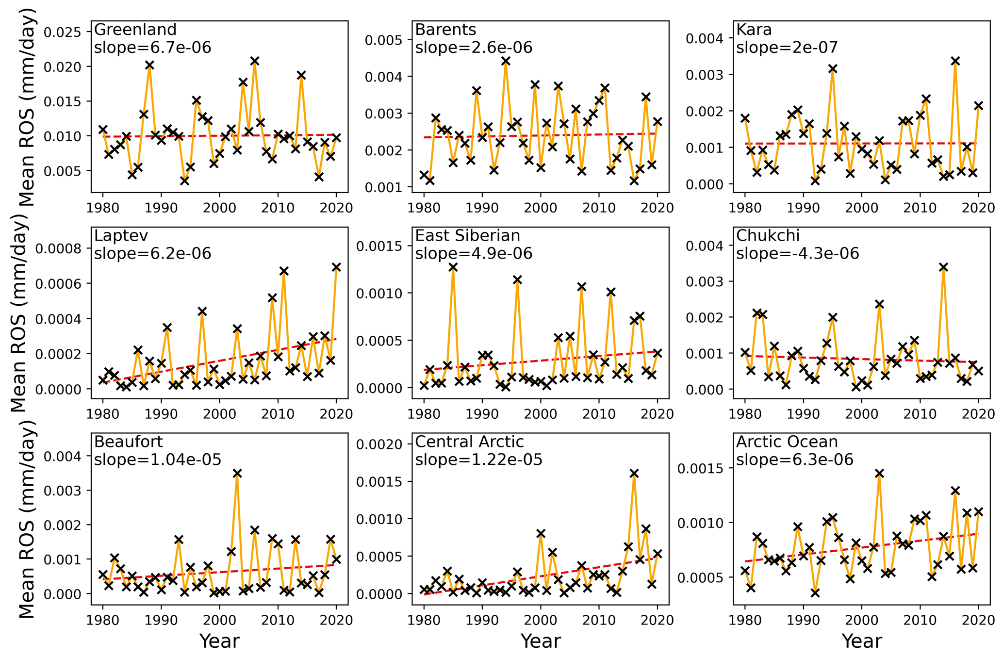
Figure A4Regionally averaged, time-averaged, non-frozen precipitation (mm d−1) over sea ice in the cold season (October through April).
The radiometers are designed to simultaneously make measurements at all three frequencies, with output provided in three individual ASCII text files stored on a USB and regularly downloaded during the MOSAiC expedition. However, there is a slight time offset in each radiometer data file. To address this, the data are first resampled to a 1 min temporal resolution, and a moving average of 30 min is applied. In addition, during the MOSAiC expedition, the GPS on the instrument did not provide accurate date tags, and all date tags had to be shifted to match the actual date the data were acquired.
During MOSAiC, a 80 cm tall pedestal was mounted to a 30 cm high komatik sled to hold the rotating positioning system on which the SBR was mounted. The instrument scanned across incidence angles ranging from 40 to 70∘ in increments of 5∘. The time to complete a full scan was approximately 5 min. At times the instrument was also set to collect data at fixed incidence angles only. Table A2 lists all the measurements acquired during Leg 5 and when the instrument was scanning versus observing at a fixed incidence angle.
Table A3 summarizes the location of the AMSR2 swath data relative to the MOSAiC floe and the times of each swath.
A3 Snow pit extra figures
We include two figures, one comparing bulk micro-CT-derived density and specific surface area (SSA) with the density cutter results. The second figure shows profiles of specific surface area and density also shown in Fig. 4 as a function of date and location.
A4 ERA5 atmospheric reanalysis data processing
We analyzed data on precipitation amount and type from the ERA5 atmospheric reanalysis at 0.25∘ spatial and 1-hourly time resolution. To characterize the precipitation at the floe we produced a time series of type and amount for the duration of the event (Fig. A3a and b).
To characterize changes in ROS over longer time periods we analyzed the same data during the cold season (October–April) between 1980–2020. After retrieving the data from the Copernicus Data Store, all values of total precipitation corresponding to places and times where the precipitation type was fully “frozen” (snow or ice pellets) were set to zero. This left the total precipitation corresponding to “wet precipitation”, i.e., rain or mixed precipitation. We also identified all precipitation falling at a rate of <0.1 mm d−1 and set this to zero. However, while trace precipitation is almost ubiquitous in ERA5 in the Arctic, almost all of this is frozen. The removal of trace precipitation did not therefore significantly impact our calculations of the total amount of ROS for each year. The remaining data were then averaged along the time axis for each year in the relevant months, only where sea ice was present (concentration >50 %) at the time of the wet precipitation. Sea ice concentration was downloaded with the ERA5 data and is derived from the EUMETSAT sea ice concentration climate data record (Tonboe et al., 2016). This produced a single, two-dimensional distribution for each year corresponding to the total wet precipitation over sea ice at each grid cell. At this point all the seasonally averaged grid cells (for each year) were spatially averaged by region (regions defined by the NSIDC; Fetterer et al., 2010). This spatial average was performed on an equal-area grid to match the grid of the mask and avoid the biassing effect of smaller ERA5 grid cells nearer the pole. This spatial averaging produced a single value for each year in each region corresponding to the average rate of wet precipitation when sea ice is present.
We finally produce an animation to illustrate the development of the weather system that brought the ROS event. To improve the visualization of the event, we employed a more aggressive trace-precipitation masking algorithm, set at 5 mm d−1. All remaining, non-frozen, non-trace precipitation is visualized with an hourly time step (Movie M1). All code for the processing and visualization of ERA5 data in this paper can be found at https://github.com/robbiemallett/ros (last access: 19 August 2021).
Data used in this paper were produced as part of the international Multidisciplinary drifting Observatory for the Study of the Arctic Climate (MOSAiC) with the tag MOSAiC20192020 and the project ID AWI PS122 00. SBR data are available from the MOSAiC Central Data Storage (MCS). KuKa data are available at http://data.bas.ac.uk/full-record.php?id=GB/NERC/BAS/PDC/01437 (Stroeve et al., 2020). KAZR and precipitation data are from the Atmospheric Radiation Measurement (ARM) user facility, a US Department of Energy (DOE) Office of Science managed by the Biological and Environmental Research Program. Meteorological data were funded by the National Science Foundation (no. OPP-1724551). Code for producing the summary plots of KuKa, SBR, and atmospheric and snow conditions can be found at https://github.com/andypbarrett/mosaic_rain_on_snow.
Animation of storm from ERA5 reanalysis included in the Supplement.
The supplement related to this article is available online at: https://doi.org/10.5194/tc-16-4223-2022-supplement.
JS wrote the manuscript with input from co-authors and analyzed the SBR data and AMSR2 brightness temperatures. VN processed the KuKa data in scan mode, while RW analyzed the KuKa waveforms as well as the CryoSat-2 waveform data (provided by SH.) TN performed the de-convolution of the KuKa data. PR provided calibrated SBR data and the impacts of the ROS on retrieved snow depth and SIC. MG provided the meteorological data for the paper, while RD provided the snow data. RM processed the ERA5 reanalysis data. AB helped to improve the figure qualities. MS, RT, GS, SH, and RR provided valuable editorial comments. Other co-authors helped collect data during MOSAiC.
At least one of the (co-)authors is a member of the editorial board of The Cryosphere. The peer-review process was guided by an independent editor, and the authors also have no other competing interests to declare.
Publisher’s note: Copernicus Publications remains neutral with regard to jurisdictional claims in published maps and institutional affiliations.
This work was carried out as part of the international Multidisciplinary drifting Observatory for the Study of the Arctic Climate (MOSAiC), MOSAiC20192020, and was funded in part by the Canada 150 Chair program (no. G00321321), the National Science Foundation (NSF; grant no. ICER 1928230), and the Natural Environment Research Council (NERC; grant nos. NE/S002510/1 and NE/L002485/1). Funding was also provided by the European Space Agency (grant no. PO 5001027396). Rosemary Willatt was partially funded by the European Union H2020-LC-CLA-2018-2019-202 CRiceS project grant no. 101003826. Vishnu Nandan was additionally supported by Canada’s Marine Environmental Observation, Prediction and Response Network (MEOPAR) postdoctoral funds. Michael Gallagher was supported by the DOE Atmospheric System Research Program (nos. DE-SC0019251 and DE-SC0021341). Philip Rostosky, Gunnar Spreen, and Linda Thielke were supported by the German Ministry for Education and Research (BMBF) through the MOSAiC IceSense project (no. 03F0866B) and by the Deutsche Forschungsgemeinschaft (DFG) through the International Research Training Group IRTG 1904 ArcTrain (no. 221211316). Mark Serreze acknowledges Scanco Medical AG for providing their newest microCT90. Mark Serreze, Ruzica Dadic, and Amy Macfarlane were supported by the European Union’s Horizon 2020 research and innovation program projects ARICE (no. 730965) for MOSAiC berth fees associated with the participation of the DEARice and by the Swiss Polar Institute grant SnowMOSAiC (no. EXF-2018-003). We thank all persons involved in the expedition of the R/V Polarstern during MOSAiC in 2019–2020 (AWI_PS122_00) as listed in Nixdorf et al. (2021). We further thank Lars Kaleschke for his calibration of the SBR instrument during Leg 3.
This research has been supported by the Canada Excellence Research Chairs, Government of Canada (grant no. G00321321); the National Science Foundation (grant no. ICER 1928230); the Natural Environment Research Council (grant nos. NE/S002510/1 and NE/L002485/1); the European Space Agency (grant no. 5001027396); the Idaho Operations Office, US Department of Energy (grant nos. DE-SC0019251 and DE-SC0021341); the Bundesministerium für Bildung und Forschung (grant no. 03F0866B); the Deutsche Forschungsgemeinschaft (grant no. 221211316); the Horizon 2020 research and innovation program (grant no. ARICE 730965); and the Swiss Polar Institute (grant no. EXF-2018-003).
This paper was edited by Yevgeny Aksenov and reviewed by two anonymous referees.
AMAP: Arctic Climate Change Update 2021: Key Trends and Impacts, Summary for Policy-makers, Arctic Monitoring and Assessment Programme (AMAP), Tromsø, 419 Norway, 16 pp., 420, https://www.amap.no/documents/download/6759/inline (last access: 30 September 2022), 2021.
Anderson, M. R.: Determination of a melt-onset date for Arctic sea-ice regions using passive-microwave data, Ann. Glaciol., 25, 382–387, https://doi.org/10.3189/S0260305500014324, 1997.
Ayhan, S., Scherr, S., Bhutani, A., Fischbach, B., Pauli, M., and Zwick, T.: Impact of Frequency Ramp Nonlinearity, Phase Noise, and SNR on FMCW Radar Accuracy, IEEE T. Microw. Theory, 64, 3290–3301, https://doi.org/10.1109/tmtt.2016.2599165, 2016.
Bartholomew, M.: Laser Disdrometer Instrument Handbook, Tech. rep., edited by: Stafford, R., ARM user facility, DOE/SC-ARM-TR-137, 2020.
Barrett, A. P., Stroeve, J. C., and Serreze, M. C.: Arctic Ocean precipitation from atmospheric reanalyses and comparisons with North Pole drifting station records, J. Geophys. Res.-Oceans, 125, https://doi.org/10.1029/2019JC015415, 2020.
Bartsch, A., Kumpula, T., Forbes, B. C., and Stammler, F.: Detection of snow surface thawing and refreezing in the Eurasian Arctic with QuikSCAT: implications for reindeer herding, Ecol. Appl., 20, 2346–2358, https://doi.org/10.1890/09-1927.1, 2010.
Budge, M. C. and Burt, M. P.: Range Correlation Effects on Phase and Amplitude Noise, Proc. Southeastcon ‘93, https://doi.org/10.1109/secon.1993.465731, 1993.
Cavalieri, D. J., Parkinson, C. L., Gloersen, P., Comiso, J. C., and Zwally, H. J.: Deriving long-term time series of sea ice cover from satellite passive-microwave multisensor data sets, J. Geophys. Res., 104, 15803–15814, https://doi.org/10.1029/1999JC900081, 1999.
Colbeck, S. C.: An overview of seasonal snow metamorphism, Rev. Geophys., 20, 45–61, https://doi.org/10.1029/RG020i001p00045, 1982a.
Colbeck, S. C.: The geometry and permittivity of snow at high frequencies, J. Appl. Phys., 53, 4495–4500, https://doi.org/10.1063/1.331186, 1982b.
Cooper, K. B., Dengler, R. J., Llombart, N., Thomas, B., Chattopadhyay, G., and Siegel, P. H.: THz Imaging Radar for Standoff Personnel Screening, IEEE Trans. Terahertz Sci. Tech., 1, 169–182, https://doi.org/10.1109/tthz.2011.2159556, 2011.
Dengler, R. J., Cooper, K. B., Chattopadhyay, G., Mehdi, I., Schlecht, E., Skalare, A., Chen, C., and Siegel, P. H.: 600 Ghz Imaging Radar With 2 Cm Range Resolution, 2007 IEEE/MTT-S Intl. Microwave Symp., https://doi.org/10.1109/mwsym.2007.380468, 2007.
Denoth, A.: Wet snow pendular regime: the amount of water in ring-shaped configurations, Cold Reg. Sci. Technol., 30, 13–18, https://doi.org/10.1016/S0165-232X(99)00007-5, 1999.
Comiso, J. C., Cavalieri, D. J., Parkinson, C. L., and Gloersen, P.: Passive microwave algorithms for sea ice concentration: A comparison of two techniques, Remote Sens. Environ., 60, 357–384, https://doi.org/10.1016/S0034-4257(96)00220-9, 1997.
Comiso, J. C., Cavalieri, D. J., and Markus, T.: Sea ice concentration, ice temperature, and snow depth using AMSR-E data, IEEE T. Geosci. Remote, 41, 243–252, https://doi.org/10.1109/TGRS.2002.808317, 2003.
Dolant, C., Langlois, A., Montpetit, A., Brucker, B., Roy, A., and Royer, A.: Development of a rain-on-snow detection algorithm using passive microwave radiometry, Hydrol. Process., 30, 3184–3196, https://doi.org/10.1002/hyp.10828, 2016.
Dou, T., Xiao, C., Liu, J., Wang, Q., Pan, S., Su, J., Yuan, X., Ding, M., Zhang, F., Xue, K., Bieniek, P. A., and Eicken, H.: Trends and spatial variation in rain-on-snow events over the Arctic Ocean during the early melt season, The Cryosphere, 15, 883–895, https://doi.org/10.5194/tc-15-883-2021, 2021.
Eppler, D. T., Farmer, L. D., Lohanick, A. W., Anderson, M. R., Cavalieri, D. J., Comiso, J., Gloersen, P., Garrity, C., Grenfell, T. C., Hallikainen, M., Maslanik, J. A., Mätzler, C., Melloh, R. A., Rubinstein, I., and Swift, C. T.: Chapter 4. Passive microwave signatures of sea ice, in: Microwave Remote Sensing of Sea Ice, Geophysical Monograph 68, edited by: Carsey, F. D., 1992.
Fetterer, F., Savoie, M., Helfrich, S., and Clemente-Colón, P.: Multisensor analyzed sea ice extent-northern hemisphere (masie-nh), Tech. rep., Technical report, National Snow and Ice Data Center, Boulder, Colorado USA, https://doi.org/10.7265/N5GT5K3K, 2010.
Forbes, B. C., Kumpula, T., Meschtyb, N., Laptander, R., Macias-Fauria, M., Zetterberg, P., Verdonen, M., Skarin, A, Kim, K.-Y., Boisvert, L. N., Stroeve J. C., and Bartsch, A.: Sea ice, rain-on-snow and tundra reindeer nomadism in Arctic Russia, Biol. Lett., 12, 20160466, https://doi.org/10.1098/rsbl.2016.0466, 2016.
Frischen, A., Hasch, J., and Waldschmidt, C.: FMCW Ramp Non-Linearity Effects and Measurement Technique for Cooperative Radar, 2015 European Radar Conference (EuRAD), https://doi.org/10.1109/eurad.2015.7346349, 2015.
Geldsetzer, T., Langlois A., and Yackel, J.: Dielectric properties of brine-wetted snow on first-year sea ice, Cold Reg. Sci. Technol., 58, 47–56, https://doi.org/10.1016/j.coldregions.2009.03.009, 2009.
Graham, R. M., Cohen, L., Petty, A. A., Boisvert, L. N., Rinke, A., Hudson, S. R., Nicolaus, M., and Granskog, M. A.: Increasing frequency and duration of Arctic winter warming events, Geophys. Res. Lett., 44, 6974–6983, https://doi.org/10.1002/2017GL073395, 2017.
Grenfell, T. C. and Putkonen, J.: A method for the detection of the severe rain‐on‐snow event on Banks Island, October 2003, using passive microwave remote sensing, Water Resour. Res., 44, W03425, https://doi.org/10.1029/2007WR005929, 2008.
Griffiths, H. D.: New Ideas in FM Radar, Elec. Comm. Eng. J., 2, 185, https://doi.org/10.1049/ecej:19900043, 1990.
Guerreiro, K., Fleury, S., Zakharova, E., Rémy, F., and Kouraev, A.: Potential for estimation of snow depth on Arctic sea ice from CryoSat-2 and SARAL/AltiKa missions, Remote Sens. Environ., 186, 339–349, https://doi.org/10.1016/j.rse.2016.07.013, 2016.
Hagenmuller, P., Matzl, M., Chambon, G., and Schneebeli, M.: Sensitivity of snow density and specific surface area measured by microtomography to different image processing algorithms, The Cryosphere, 10, 1039–1054, https://doi.org/10.5194/tc-10-1039-2016, 2016.
Harasyn, M. L., Isleifson, D., Chan, W., and Barber, D. G.: Multi-scale observations of the co-evolution of sea ice thermophysical properties and microwave brightness temperatures during the summer melt period in Hudson Bay, Elementa: Science of the Anthropocene, https://doi.org/10.1525/elementa.412, 2020.
Hersbach, H., Bell, B., Berrisford, P., Biavati, G., Horányi, A., Muñoz Sabater, J., Nicolas, J., Peubey, C., Radu, R., Rozum, I., Schepers, D., Simmons, A., Soci, C., Dee, D., and Thépaut, J. N.: ERA5 hourly data on single levels from 1979 to present, Copernicus Climate Change Service (C3S) Climate Data Store (CDS), https://doi.org/10.24381/cds.adbb2d47, 2018.
Ivanova, N., Pedersen, L. T., Tonboe, R. T., Kern, S., Heygster, G., Lavergne, T., Sørensen, A., Saldo, R., Dybkjær, G., Brucker, L., and Shokr, M.: Inter-comparison and evaluation of sea ice algorithms: towards further identification of challenges and optimal approach using passive microwave observations, The Cryosphere, 9, 1797–1817, https://doi.org/10.5194/tc-9-1797-2015, 2015.
Kaleschke, L., Tian-Kunze, X., Maaß, N., Beitsch, A., Wernecke, A., Miernecki, M., Müller, G., Fock, B. H., Gierisch, A. M. U., Schlünzen, K. H., Pohlmann, T., Dobrynin, M., Hendricks, S., Asseng, J., Gerdes, R., Jochmann, P., Reimer, N., Holfort, J., Melsheimer, C., Heygster, G., Spreen, G., Gerland, S., King, J., Skou, N., Schmidl Søbjærg, S., Haas, C., Richter, F., and Casal, T.: SMOS sea ice product: Operational application and validation in the Barents Sea marginal ice zone, Remote Sens. Environ., 180, 264–273, https://doi.org/10.1016/j.rse.2016.03.009, 2016.
Kerbrat, M., Pinzer, B., Huthwelker, T., Gäggeler, H. W., Ammann, M., and Schneebeli, M.: Measuring the specific surface area of snow with X-ray tomography and gas adsorption: comparison and implications for surface smoothness, Atmos. Chem. Phys., 8, 1261–1275, https://doi.org/10.5194/acp-8-1261-2008, 2008.
Kim, Y. S., Onstott, R., and Moore, R.: Effect of a snow cover on microwave backscatter from sea ice, IEEE J. Oceanic Eng., 9, 383–388, https://doi.org/10.1109/JOE.1984.1145649, 1984.
King, J., Skourup, H., Hvidegaard, S. M., Rösel, A., Gerland, S., Spreen, G., Polashenski, C., Helm V., and Liston, G. E.: Comparison of freeboard retrieval and ice thickness calculation from ALS, ASIRAS, and CryoSat-2 in the Norwegian Arctic to field measurements made during the N-ICE2015 expedition, J. Geophys. Res.-Oceans, 123, 1123–1141, https://doi.org/10.1002/2017JC013233, 2018.
Krumpen, T., Birrien, F., Kauker, F., Rackow, T., von Albedyll, L., Angelopoulos, M., Belter, H. J., Bessonov, V., Damm, E., Dethloff, K., Haapala, J., Haas, C., Harris, C., Hendricks, S., Hoelemann, J., Hoppmann, M., Kaleschke, L., Karcher, M., Kolabutin, N., Lei, R., Lenz, J., Morgenstern, A., Nicolaus, M., Nixdorf, U., Petrovsky, T., Rabe, B., Rabenstein, L., Rex, M., Ricker, R., Rohde, J., Shimanchuk, E., Singha, S., Smolyanitsky, V., Sokolov, V., Stanton, T., Timofeeva, A., Tsamados, M., and Watkins, D.: The MOSAiC ice floe: sediment-laden survivor from the Siberian shelf, The Cryosphere, 14, 2173–2187, https://doi.org/10.5194/tc-14-2173-2020, 2020.
Kwok, R., Kacimi, S., Webster, M. A., Kurtz, N. T., and Petty, A. A.: Arctic snow depth and sea ice thickness from ICESat-2 and CryoSat-2 freeboards: A first examination. J. Geophys. Res.-Oceans, 125, https://doi.org/10.1029/2019JC016008, 2020.
Landy, J. C., Petty, A. A., Tsamados, M., and Stroeve, J. C.: Sea ice roughness overlooked as key source of uncertainty in CryoSat-2 ice freeboard retrievals, J. Geophys. Res.-Oceans, https://doi.org/10.1029/2019JC015820, 2020.
Langlois, A., Johnson, C.-A., Montpetit, B., Royer, A., Blukacz-Richards, E. A., Neave, E., et al.: Detection of rain-on-snow (ROS) events and ice layer formation using passive microwave radiometry: A context for Peary caribou habitat in the Canadian Arctic, Remote Sens. Environ., 189, 84–95, https://doi.org/10.1016/j.rse.2016.11.006, 2017.
Laxon, S.: Sea ice extent mapping using the ERS-1 radar altimeter, EARSeL Adv. Remote Sens., 3, 112–116, 1994.
Legagneux, L., Cabanes, A., and Dominé, F.: Measurement of the specific surface area of 176 snow samples using methane adsorption at 77 K, J. Geophys. Res.-Atmos., 107, https://doi.org/10.1029/2001JD001016, 2002.
Li, D., Lettenmaier, D. P., Margulis, S. A., and Andreadis, K.: The role of rain on-snow in flooding over the conterminous United States, Water Resour. Res., 55, 8492–8513, https://doi.org/10.1029/2019WR024950, 2019.
Liston, G. E. and Hiemstra, C. A.: The changing cryosphere: Pan-Arctic snow trends (1979–2009), J. Climate, 24, 5691–5712, https://doi.org/10.1175/JCLI-D-11-00081.1, 2011.
Luck, D. G. C.: Frequency Modulated Radar, New York, McGraw-Hill, (OCoLC) 609158063, 1949.
Mallett, R. D. C., Lawrence, I. R., Stroeve, J. C., Landy, J. C., and Tsamados, M.: Brief communication: Conventional assumptions involving the speed of radar waves in snow introduce systematic underestimates to sea ice thickness and seasonal growth rate estimates, The Cryosphere, 14, 251–260, https://doi.org/10.5194/tc-14-251-2020, 2020.
Markus, T. and Cavalieri, D. J.: Snow Depth Distribution Over Sea Ice in the Southern Ocean from Satellite Passive Microwave Data, in: Antarctic Sea Ice: Physical Processes, Interactions and Variability, edited by: Jeffries, M. O., American Geophysical Union, Washington, DC, 19–39, 1998.
Markus, T. and Cavalieri, D. J.: The AMSR-E NT2 sea ice concentration algorithm: Its basis and implementation, J. Rem. Sens. Soc. Japan, 29, 216–225, https://doi.org/10.11440/rssj.29.216, 2009.
Markus, T., Stroeve, J. C., and Miller, J.: Recent changes in Arctic sea ice melt onset, freezeup, and melt season length, J. Geophys. Res.-Oceans, 114, https://doi.org/10.1029/2009JC005436, 2009.
McCrystall, M. R., Stroeve, J., Serreze, M., Forbes, B. C., Screen, J. A.: New climate models reveal faster and larger increases in Arctic precipitation than previously projected, Nat. Commun., 12, 6765, https://doi.org/10.1038/s41467-021-27031-y, 2021.
Meredith, M., Sommerkorn, M., Cassotta, S., Derksen, C., Ekaykin, A., Hollowed, A., Kofinas, G., Mackintosh, A., Melbourne-Thomas, J., Muelbert, M. M. C., Ottersen, G., Pritchard, H., and Schuur, E. A. G.: Polar Regions, in: IPCC Special Report on the Ocean and Cryosphere in a Changing Climate, edited by: Pörtner, H.-O., Roberts, D. C., Masson Delmotte, V., Zhai, P., Tignor, M., Poloczanska, E., Mintenbeck, K., Alegría, A., Nicolai, M., Okem, A., Petzold, J., Rama, B., and Weyer, N. M., 2019.
Meta, A., Hoogeboom, P., and Ligthart, L.: Range Non-Linearities Correction in FMCW SAR, IEEE Intl. Symp. Geosci. Rem. Sens., https://doi.org/10.1109/igarss.2006.108, 2006.
Meta, A., Hoogeboom, P., and Ligthart, L. P.: Signal Processing for Fmcw Sar, IEEE T. Geosci. Remote, 45, 3519–3532, https://doi.org/10.1109/tgrs.2007.906140, 2007.
Mortin, J., Schrøder, T. M., Walløe Hansen, A., Holt, B., and McDonald, K. C.: Mapping of seasonal freeze-thaw transitions across the pan-Arctic land and sea ice domains with satellite radar, J. Geophys. Res.-Oceans, 117, https://doi.org/10.1029/2012JC008001, 2012.
Mortin, J., Howell, S. E., Wang, L., Derksen, C., Svensson, G., Graversen, R. G., and Schrøder T. M.: Extending the QuikSCAT record of seasonal melt-freeze transitions over Arctic sea ice using ASCAT, Remote Sens. Environ., 141, 214–230, https://doi.org/10.1016/j.rse.2013.11.004, 2014.
Nandan, V., Geldsetzer, T., Yackel, J., Mahmud, M., Scharien, R., Howell, S., King, J., Ricker, R., and Else, B.: Effect of snow salinity on CryoSat2 Arctic first year sea ice freeboard measurements, Geophys. Res. Lett., 44, 10–419, https://doi.org/10.1002/2017GL074506, 2017.
Nandan, V., Scharien, R. K., Geldsetzer, T., Kwok, R., Yackel, J. J., Mahmud, M. S., Rösel, A., Tonboe, R., Granskog, M., Willatt, R., Stroeve, J., Nomura, D., and Frey, M.: Snow Property Controls on Modeled Ku-Band Altimeter Estimates of First-Year Sea Ice Thickness: Case Studies From the Canadian and Norwegian Arctic, IEEE J. Sel. Top. Appl., 13, 1082–1096, https://doi.org/10.1109/JSTARS.2020.2966432, 2020.
Nghiem, S. V., Kwok, R., Yueh, S. H., and Drinkwater, M. R.: Polarimetric signatures of sea ice: 2. Experimental observations, J. Geophys. Res.-Oceans, 100, 13681–13698, 1995.
Nicolaus, M., Perovich, D. K., Spreen, G., Granskog, M. A., von Albedyll, L., Angelopoulos, M., et al.: Overview of the MOSAiC expedition: Snow and sea ice, Elem. Sci. Anth., 10, 000046, https://doi.org/10.1525/elementa.2021.000046, 2022.
Nixdorf, U., Dethloff, K., Rex, M., Shupe, M., Sommerfeld, A., Perovich, D., Nicolaus, M., Heuzé, C., Rabe, B., Loose, B., Damm, E., Gradinger, R., Fong, A., Maslowski, W., Rinke, A., Kwok, R., Spreen, G., Wendisch, M., Herber, A., Hirsekorn, M., Mohaupt, V., Frickenhaus, S., Immerz, A., Weiss-Tuider, K., König, B., Mengedoht, D., Regnery, J., Gerchow, P., Ransby, D., Krumpen, T., Morgenstern, A., Haas, C., Kanzow, T., Rack, F. R., Saitzev, V., Sokolov, V., Makarov, A., Schwarze, S., Wunderlich, T., Wurr, K., and Boetius, A.: MOSAiC extended acknowledgement, Zenodo, https://doi.org/10.5281/zenodo.5179739, 2021.
Onstott, R. G.: SAR and Scatterometer Signatures of Sea Ice, in: Microwave Remote Sensing of Sea Ice, edited by: Carsey, F. D., https://doi.org/10.1029/GM068p0073, 1992.
Peacock, N. R. and Laxon, S. W.: Sea surface height determination in the Arctic Ocean from ERS altimetry, J. Geophys. Res., 109, https://doi.org/10.1029/2001JC001026, 2004.
Piper, S. O.: Homodyne FMCW Radar Range Resolution Effects With Sinusoidal Nonlinearities in the Frequency Sweep, Proc. Intl. Radar Con., https://doi.org/10.1109/radar.1995.522609, 1995.
Putkonen, J. and Roe, G.: Rain-on-snow events impact soil temperatures and affect ungulate survival, Geophys. Res. Lett., 30, 1188, https://doi.org/10.1029/2002GL016326, 2003.
Putkonen, J., Grenfell, T. C., Rennert, K., Bitz, C., Jacobson, P., and Russell, D.: Rain on Snow: Little Understood Killer in the North, Eos Trans. AGU, 90, 221–222, https://doi.org/10.1029/2009EO260002, 2009.
Radiometrics: AC1900 19 GHz, AC3700 37 GHz, and AC8900 89 GHz dual polarization radiometers, Radiometric Corporation, User Guide, 2004.
Rennert, K. J., Roe, G., Putkonen, J., and Bitz, C. M.: Soil thermal and ecological impacts of rain on snow events in the circumpolar Arctic, J. Climate, 22, 2302–2315, https://doi.org/10.1175/2008JCLI2117.1, 2009.
Rostosky, P., Spreen, G., Farrell, S. L., Frost, T., Heygster, G., and Melsheimer, C.: Snow depth retrieval on Arctic sea ice from passive microwave radiometers-Improvements and extensions to multiyear ice using lower frequencies, J. Geophys. Res.-Oceans, 123, 7120–7138, https://doi.org/10.1029/2018JC014028, 2018.
Seifert, W. J. and Langleben, M. P.: Air drag coefficient and roughness length of a cover of sea ice, J. Geophys. Res., 77, 2708–2713, https://doi.org/10.1029/JC077i015p02708, 1972.
Serreze, M. C., Barrett, A. P., Stroeve, J. C., Kindig, D. N., and Holland, M. M.: The emergence of surface-based Arctic amplification, The Cryosphere, 3, 11–19, https://doi.org/10.5194/tc-3-11-2009, 2009.
Shupe, M., Costa, D., Chu, D., Costa, D., Cox, C., Creamean, J., de Boer, G., Detholff, K., Englemann, R., Gallagher, M., Hunke, E., Maslowski, W., McComiskey, A., Osborn, J., Persson, O., Powers, H., Pratt, K., Randall, D., Solomon, A., Tjernstrom, M., Turner, D., Uin, J., Uttal, T., Verlinde, J., and Wagner, D.: Multidisciplinary drifting Observatory for the study of Arctic climate (MOSAiC) field campaign report, U.S. Department of Energy, DOE/SC-ARM-21-007, 25 pp., https://www.arm.gov/publications/programdocs/doe-sc-arm-21-007.pdf, last access: 12 August 2021.
Shupe, M. D., Uttal, T., and Matrosov, S. Y.: Arctic Cloud Microphysics Retrievals from Surface-Based Remote Sensors at SHEBA, J. Appl. Meteorol., 44, 1544–1562, https://doi.org/10.1175/JAM2297.1, 2005.
Spreen, G., Kaleschke L., and Heygster, G.: Sea ice remote sensing using AMSRE 89-GHz channels J. Geophys. Res.-Oceans, 113, https://doi.org/10.1029/2005JC003384, 2008.
Stirling, I. and Smith, T. G.: Implications of warm temperatures and an unusual rain event for the survival of ringed seals on the coast of southeastern Baffin Island, Arctic, 57, 59–67, https://doi.org/10.14430/arctic483, 2004.
Stove, A. G.: Linear FMCW Radar Techniques, IEEE Proc. Radar Sign. Proces., 139, 343–350, https://doi.org/10.1049/ip-f-2.1992.0048, 1992.
Stroeve, J., Nandan, V., Willatt, R., Tonboe, R., Hendricks, S., Ricker, R., Mead, J., Mallett, R., Huntemann, M., Itkin, P., Schneebeli, M., Krampe, D., Spreen, G., Wilkinson, J., Matero, I., Hoppmann, M., and Tsamados, M.: Surface-based Ku- and Ka-band polarimetric radar for sea ice studies, The Cryosphere, 14, 4405–4426, https://doi.org/10.5194/tc-14-4405-2020, 2020 (data available at: http://data.bas.ac.uk/full-record.php?id=GB/NERC/BAS/PDC/01437, last acess: 30 September 2022).
Tjuatja, S., Fung, A. K., and Bredow, J.: A scattering model for snow-covered sea ice, IEEE T. Geosci. Remote, 30, 804–810, https://doi.org/10.1109/36.158876, 1992.
Tietsche, S., Alonso-Balmaseda, M., Rosnay, P., Zuo, H., Tian-Kunze, X., and Kaleschke, L.: Thin Arctic sea ice in L-band observations and an ocean reanalysis, The Cryosphere, 12, 2051–2072, https://doi.org/10.5194/tc-12-2051-2018, 2018.
Tilling, R. L., Ridout, A., and Shepherd, A.: Estimating Arctic sea ice thickness and volume using CryoSat-2 radar altimeter data, Adv. Space Res., 62, 1203–1225, https://doi.org/10.1016/j.asr.2017.10.051, 2018.
Tonboe, R. T., Eastwood, S., Lavergne, T., Sørensen, A. M., Rathmann, N., Dybkjær, G., Pedersen, L. T., Høyer, J. L., and Kern, S.: The EUMETSAT sea ice concentration climate data record, The Cryosphere, 10, 2275–2290, https://doi.org/10.5194/tc-10-2275-2016, 2016.
Tonboe, R. T., Nandan, V., Yackel, J., Kern, S., Pedersen, L. T., and Stroeve, J.: Simulated Ka- and Ku-band radar altimeter height and freeboard estimation on snow-covered Arctic sea ice, The Cryosphere, 15, 1811–1822, https://doi.org/10.5194/tc-15-1811-2021, 2021.
Ulaby, F. T. and Stiles, W. H.: The active and passive microwave response to snow parameters: 2. Water equivalent of dry snow, J. Geophys. Res., 85, 1045–1049, https://doi.org/10.1029/JC085iC02p01045, 1980.
Voss, S., Heygster, G., and Ezraty, R.: Improving sea ice type discrimination by the simultaneous use of SSM/I and scatterometer data, Polar Res., 22, 35–42, https://doi.org/10.3402/polar.v22i1.6441, 2003.
Vossiek, M., Heide, P., Nalezinski, M., and Magori, V.: Novel FMCW Radar System Concept With Adaptive Compensation of Phase Errors, 26th European Microwave Conf., 6–13 September 1996 in Prague, Czech, https://doi.org/10.1109/euma.1996.337536, 1996.
Vuyovich, C. M., Jacobs, J. M., Hiemstra, C. A., and Deeb, E. J.: Effect of spatial variability of wet snow on modeled and observed microwave emissions, Remote Sens. Environ., 198, 310–320, https://doi.org/10.1016/j.rse.2017.06.016, 2017.
Wagner, D. N., Shupe, M. D., Cox, C., Persson, O. G., Uttal, T., Frey, M. M., Kirchgaessner, A., Schneebeli, M., Jaggi, M., Macfarlane, A. R., Itkin, P., Arndt, S., Hendricks, S., Krampe, D., Nicolaus, M., Ricker, R., Regnery, J., Kolabutin, N., Shimanshuck, E., Oggier, M., Raphael, I., Stroeve, J., and Lehning, M.: Snowfall and snow accumulation during the MOSAiC winter and spring seasons, The Cryosphere, 16, 2373–2402, https://doi.org/10.5194/tc-16-2373-2022, 2022.
Webb, R. W., Marziliano, A., McGrath, D., Bonnell, R., Meehan, T. G., Vuyovich, C., and Marshall, H. P.: In Situ Determination of Dry and Wet Snow Permittivity: Improving Equations for Low Frequency Radar Applications, Remote Sensing, 13, 4617, doi.org/10.3390/rs13224617, 2021.
Westermann, S., Boike, J., Langer, M., Schuler, T. V., and Etzelmüller, B.: Modeling the impact of wintertime rain events on the thermal regime of permafrost, The Cryosphere, 5, 945–959, https://doi.org/10.5194/tc-5-945-2011, 2011.
Willatt, R. C., Giles, K. A., Laxon, S. W., Stone-Drake, L., and Worby, A. P.: Field investigations of Ku-band radar penetration into snow cover on Antarctic sea ice, IEEE T. Geosci. Remote, 48, 365–372, https://doi.org/10.1109/TGRS.2009.2028237, 2010.
Zhaodu, Z., Weidong, Y., Xinggan, Z., and Xiaohui, Q.: A Correction Method for Distortions in FMCW Imaging System, Proc. IEEE 1996 Natl. Aerospace Elec. Conf. NAECON, 20–22 May 1996, https://doi.org/10.1109/naecon.1996.517666, 1996.
- Abstract
- Introduction
- Instrumentation and data
- ROS event: meteorological and surface conditions
- Impacts of ROS on radar backscatter and microwave emission
- Implications
- Changes in ROS
- Conclusions
- Appendix A: Data processing and figures in the Supplement
- Code and data availability
- Video supplement
- Author contributions
- Competing interests
- Disclaimer
- Acknowledgements
- Financial support
- Review statement
- References
- Supplement