Variability in Antarctic surface climatology across regional climate models and reanalysis datasets

Regional climate models (RCMs) and reanalysis datasets provide valuable information for assessing the vulnerability of ice shelves to collapse over Antarctica, which is important for future global sea level rise estimates. Within this context, this paper examines variability in snowfall, near-surface air temperature and melt across products from the Met Office Unified Model (MetUM), Regional Atmospheric Climate Model (RACMO) and Modèle Atmosphérique Régional (MAR) RCMs, as well as the ERA-Interim and ERA5 reanalysis datasets. Seasonal and trend decomposition using LOESS (STL) is applied to split the monthly time series at each model grid cell into trend, seasonal and residual components. Significant systematic differences between outputs are shown for all variables in the mean and in the seasonal and residual standard deviations, occurring at both large and fine spatial scales across Antarctica. Results imply that differences in the atmospheric dynamics, parametrisation, tuning and surface schemes between models together contribute more significantly to large-scale variability than differences in the driving data, resolution, domain specification, ice sheet mask, digital elevation model and boundary conditions. Despite significant systematic differences, high temporal correlations are found for snowfall and near-surface air temperature across all products at fine spatial scales. For melt, only moderate correlation exists at fine spatial scales between different RCMs and low correlation between RCM and reanalysis outputs. Root mean square deviations (RMSDs) between all outputs in the monthly time series for each variable are shown to be significant at fine spatial scales relative to the magnitude of annual deviations. Correcting for systematic differences results in significant reductions in RMSDs, suggesting the importance of observations and further development of bias-correction techniques.

1 Introduction

The largest source of uncertainty in 2100 sea level rise (SLR) projections, for a given representative concentration pathway (RCP), is from the contribution of ice sheets (Kopp et al., 2017). Non-linear instabilities in the Greenland and Antarctic ice sheets give long tails to their SLR probability projections. For example, under RCP8.5 the median SLR from Antarctica is projected to be of the order of 20 cm, while the 95th percentile is 6 times higher, at 130 cm (Bamber et al., 2019). The Antarctic continent is fringed by ice shelves, which act like “ice dams”, slowing down the flow of inland ice towards the sea (Rignot et al., 2004; Scambos et al., 2004). The stability of the ice shelves under a warming climate strongly determines the rate of SLR from Antarctica, and it is, in part, the difficulty of modelling their complex physical dynamics, leading to retreat/collapse, that results in the large uncertainty in estimates of future SLR (Bulthuis et al., 2019).

The primary method of ice shelf retreat, when considered across the entire ice sheet, is currently through oceanic basal melting (Pritchard et al., 2012; Paolo et al., 2015), although notable exceptions are recent and dramatic collapse events, such as the disintegration of the Larsen B ice shelf in 2002, which are linked to anomalous atmospheric conditions through the process of melt-induced hydrofracture (Scambos et al., 2000; van den Broeke, 2005; Bell et al., 2018). Anomalously high near-surface air temperatures (leading to enhanced melt events), as well as low accumulation (leading to reduced pore space of surface snow), result in greater lateral propagation of meltwater into crevasses across the ice shelf, which then deepen due to increased hydrostatic pressure (Kuipers Munneke et al., 2014). This process reduces the structural integrity of the ice shelf and, in addition to fractures created through supraglacial lake filling and drainage, can eventually lead to collapse (Banwell et al., 2013; Kuipers Munneke et al., 2014). Recent ice sheet modelling studies indicate the critical importance of atmosphere-driven hydrofracture events in distant-past SLR variation (Pollard et al., 2015) and near-future 2100–2300 SLR estimates, particularly under high-emission scenarios (DeConto et al., 2021). Comprehensive spatiotemporal estimates of near-surface air temperature over Antarctica, as well as the accumulation of snowfall and quantity of meltwater, are thus important for SLR predictions and are typically provided by regional climate models (RCMs; van Wessem et al., 2018; Agosta et al., 2019; Mottram et al., 2021).

RCMs are limited-area, physically based, nested models driven at the boundaries by lower-resolution global climate models (GCMs) or reanalysis datasets. The high resolution available from RCMs is important for capturing fine-scale climatic processes in regions of complex topography, such as föhn winds that occur over ice shelves on the Antarctic Peninsula (Luckman et al., 2014). The region-specific domain enables the set-up and physical schemes of the RCM to be polar optimised (Orr et al., 2021). In addition, further added value of RCMs is provided through inclusion of region-specific, sophisticated surface and sub-surface schemes that capture processes such as meltwater percolation (Ettema et al., 2010; Datta et al., 2019; Walters et al., 2017). Despite these features, RCMs still exhibit significant systematic errors precluding their direct interpretation in climate change impact studies (CCISs) (Christensen et al., 2008; Ehret et al., 2012).

The atmospheric model dynamics, surface scheme, parametrisation, driving data, boundary conditions, domain, resolution and orography are all examples of components that contribute to systematic error (Ehret et al., 2012; Giorgi, 2019; Mottram et al., 2021). This paper examines the magnitude and spatial distribution of systematic differences in an ensemble of RCM simulations for Antarctic-wide, 1980–2018 estimates of snowfall, near-surface air temperature and meltwater. The relative contributions from different components of the simulations, such as the atmospheric model physics, are discussed. Comparisons of Antarctic-wide RCM simulations of recent historic surface climatology are present in the literature (Mottram et al., 2021; van Wessem et al., 2018; Agosta et al., 2019), although the focus is predominantly on surface mass balance (SMB). Surface melt flux, when integrated over the Antarctic ice sheet, only represents a small fraction of the total SMB, which is determined predominantly by the flux of snowfall (Lenaerts et al., 2012b; Agosta et al., 2019). This paper provides the first inter-comparison of recent historic Antarctic-wide RCM simulations framed within the context of ice shelf instability and collapse events, giving specific focus to variability in near-surface air temperature, snowfall and meltwater.

Table 1 The two reanalysis datasets and six RCM simulation outputs compared in the paper. The label with which each simulation is referred to in the paper is given.

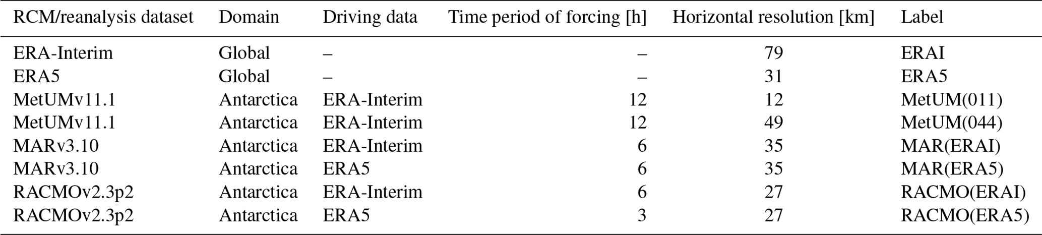
Six Antarctic-wide RCM simulations are compared, two from each of the Met Office Unified Model version 11.1 (MetUMv11.1), the Modèle Atmosphérique Régional version 3.10 (MARv3.10) and the Regional Atmospheric Climate Model version 2.3p2 (RACMOv2.3p2). Comparisons are also made to the reanalysis driving data of ERA-Interim and ERA5. The resulting eight Antarctic-wide datasets analysed in this paper are given in Table 1. MARv3.10 and RACMOv2.3p2 are both hydrostatic models specifically developed for use over polar regions, and their outputs from Antarctic-wide simulations have been rigorously compared to one another and against observations (Lenaerts et al., 2012b; van Wessem et al., 2018; Agosta et al., 2019). MetUMv11.1 is not specifically developed with a focus on the polar regions, although it is a non-hydrostatic model meaning it can be run at and simulate atmospheric circulation features at sub-kilometre resolutions (Orr et al., 2021), whereas MAR and RACMO are limited to maximum resolutions of 5–10 km horizontal grid spacing (van Wessem et al., 2016; Datta et al., 2019). Another feature of particular note in the MetUM simulations is that a “zero-layer” surface scheme is used, which has been identified as a major deficiency in simulations compared with the multi-layer schemes included in MAR and RACMO due to impacts such as that on heat transfer and not representing the insulating properties of the column of snow (Slater et al., 2017; Walters et al., 2017). It is therefore expected that the MetUM, as well as the reanalysis datasets ERA-Interim and ERA5 that both use a single tile to represent snow, will produce much less physically realistic evaluations of melt than MAR and RACMO. Further details on key differences in the model specifications for the simulations analysed in this paper are presented in Sect. 2.

Historic evaluation simulations are chosen to remove dependency on emission scenarios, which have been shown to introduce divergent trajectories of variables such as melt (Trusel et al., 2015; Gilbert and Kittel, 2021; Kittel et al., 2021). Comparisons to observations are not included due to the sparse nature of observations available over Antarctica. Papers including observations typically require comparisons to be made across elevation bins (Mottram et al., 2021; van Wessem et al., 2018; Agosta et al., 2019). In this paper comparisons are made at a 12 km grid-cell level, and it is shown that variability between the simulations has greater dependency on the latitude and longitude location than on elevation. To study the temporal dependence of variability time series, decomposition is applied, separating the signal at each location into an annual, seasonal and residual component. These components are driven by different physical processes, and the previous inter-comparison papers cited have not focused on examining variability at different temporal scales. Finally, despite the primary motivation for this paper focusing on surface climatology over ice shelves, the analysis is extended to the whole Antarctic ice sheet and surrounding Southern Ocean. This is done to aid discussion, as surface climatology over the ice shelves is influenced by the behaviour of the models over the rest of the domain, and extending the analysis provides insights useful for studies not only focused on ice shelves, thus increasing the scope of the work.

2 Reanalysis datasets and RCM specifications

The ensemble of Antarctic-wide RCM simulations examined in this paper is part of the Coordinated Regional Climate Downscaling Experiment (CORDEX; https://cordex.org/, last access: 1 March 2022), which is a global project that provides coordinated sets of RCM simulations worldwide. The model specifications for each of the RCM simulations in the chosen ensemble, as well as for the ERA-Interim and ERA5 reanalysis products, are detailed here. There are significant differences, with some of the key aspects being the following: different atmospheric dynamics components; different surface schemes; differences in the vertical and horizontal resolutions, with particular interest in the performance of the high-resolution 12 km MetUM simulation against the low-resolution 49 km MetUM simulation; differences in the driving data, with particular interest in the two RACMO and two MAR simulations that are otherwise identical; and differences in the digital elevation models (DEMs) and masks used by each model, with MAR and RACMO using comparatively similar DEMs, while the MetUM uses a DEM similar to that of ERA5 (Fig. C1).

2.1 ERA-Interim and ERA5

ERA-Interim, produced by the European Centre for Medium-Range Weather Forecasts (ECMWF), is a global reanalysis dataset spanning 1979–2019 with 6 h temporal resolution and approximately uniform horizontal resolution of 79 km spacing and 60 vertical levels up to 10 Pa (Dee et al., 2011). ERA-Interim used to be world leading and is included as the specified driving data in the base criteria for the CORDEX simulations but has since been superseded by ERA5, also produced by ECMWF (Hersbach et al., 2020), with a number of ERA5-driven simulations also included in the Antarctic CORDEX ensemble of RCM outputs. The ERA5 reanalysis dataset uses the updated Cycle 41r2 version of the Integrated Forecasting System (IFS) numerical weather prediction (NWP) model, with significant developments to model physics and assimilation methods (Hersbach et al., 2020). It spans 1950–present with an enhanced single hourly temporal resolution, horizontal resolution of 31 km and 139 vertical levels up to 1 Pa. In addition, ERA5 has uncertainty estimates derived from an ensemble of 10 data assimilations performed at a 3 h temporal resolution and horizontal resolution of 63 km. The elevation used by ERA-Interim comes from interpolating the GTOPO30 elevation product (ECMWF, 2009), whereas for ERA5 surface elevation is derived from interpolation of a combination of the SRTM30 elevation product along with other surface elevation datasets (ECMWF, 2016). The coupled surface schemes used for ERA-Interim and ERA5 are the Tiled ECMWF Scheme for Surface Exchanges over Land (TESSEL) and updated HTESSEL (TESSEL incorporating land surface hydrology) schemes respectively; both use a single tile to represent snow, while one of the major differences is that HTESSEL allows surface runoff (Balsamo et al., 2009).

2.2 MAR

MAR is a hydrostatic RCM, specifically developed for the polar areas (Fettweis et al., 2013). The Antarctic-wide simulations analysed in this paper have a spatial horizontal resolution of 35 km with a vertical resolution of 24 atmospheric levels. Specific details of the atmospheric component of MAR can be found in Gallée and Schayes (1994) and Gallée (1995). The atmospheric model is fully coupled to the 1-D SISVAT (Soil Ice Snow Vegetation Atmosphere Transfer) surface scheme (Fettweis et al., 2013, 2017), which uses the Crocus multi-layer surface snow model (Brun et al., 1992) that contains subroutines for processes such as snow metamorphism as well as meltwater runoff, retention, refreezing and percolation. SISVAT does not include a full radiative transfer scheme in snow/ice, and surface albedo is parametrised as a function of snow grain properties (Tedesco et al., 2016). The relaxation technique is used to apply LBCs (lateral boundary conditions) from the driving data every 6 h, and spectral nudging is used to constrain the large-scale behaviour in the upper atmosphere. The two Antarctic-wide MAR simulations studied in this paper are identical apart from differing driving data from ERA-Interim and ERA5 respectively. The orography used in the simulations is from Bedmap2 (Fretwell et al., 2013). For further detail on MAR and the specific version used to generate the output examined in this paper (MARv3.10), the reader is referred to Agosta et al. (2019) and Mottram et al. (2021).

2.3 RACMO

RACMO is a hydrostatic RCM with a polar version developed to represent the climate specifically over ice sheets (Van Meijgaard et al., 2008). The RCM uses the dynamical core from HIRLAM (High Resolution Limited Area Model) (Undén et al., 2002) and the physics package CY33R1 version of the Integrated Forecasting System (IFS) NWP model from ECMWF. The Antarctic-wide simulations analysed in this paper have a spatial horizontal resolution of 27 km with a vertical resolution of 40 atmospheric levels. The simulations include a multi-layer snow scheme that simulates hydrological processes such as melt, percolation, refreezing and runoff as well as firn densification (Ettema et al., 2010). In addition, a drifting snow scheme simulates movement of snow from surface winds across the ice sheet (Lenaerts et al., 2010, 2012a). A snow albedo scheme is implemented, which uses snow grain size as a prognostic variable as well as cloud optical thickness and the solar zenith angle to estimate albedo (Munneke et al., 2011). The relaxation technique is used to apply LBCs from the driving data every 6 h for the RACMO simulation driven by ERA-Interim and every 3 h for the simulation driven by ERA5, and spectral nudging is used to constrain the large-scale behaviour in the upper atmosphere. The two simulations studied are identical apart from differing driving data from ERA-Interim and ERA5 respectively. The orography used in the simulations is the same as from Bamber et al. (2009). For further detail on RACMO and the specific version used to generate the output examined in this paper (RACMOv2.3p2), the reader is referred to van Wessem et al. (2018) and Mottram et al. (2021).

2.4 MetUM

The MetUM is a non-hydrostatic climate model, not specifically developed or optimised for use over the polar regions but adapted in these simulations for use over Antarctica (Orr et al., 2021). The Global Atmosphere 6.0 and Joint UK Land Environment Simulator (JULES) Global Land configuration is used, which is suitable for the regional configuration of the MetUM at grid scales of 10 km or coarser (Walters et al., 2017). JULES is used with the option of a comparatively simple zero-layer snow/soil composite scheme that does not capture processes such as refreezing of meltwater (Best et al., 2011). The two Antarctic-wide MetUM simulations analysed in this paper are identical apart from their spatial horizontal resolutions of 12 and 49 km respectively; both have a common vertical resolution of 70 atmospheric levels. These limited-area, regional simulations are nested inside the global model configuration of the MetUM, which is itself forced using ERA-Interim reanalysis data and follows a 12 h re-initialisation procedure that constrains the large-scale circulation in the interior of the domain and prevents it from drifting too far from the driving data (Gilbert et al., 2021). The global MetUM model runs for 24 h periods, with a re-initialisation happening throughout the domain every 12 h and boundary conditions for the nested run saved each hour. The first 12 h of each 24 h run is discarded as spin-up, while the second 12 h of each run is kept as output and stitched together with following runs. The orography used in the simulations is the MetUM standard GLOBE 1 km dataset (GLOBE, 1999).

3 Comparison method

The RCM simulations examined in this paper all use an equatorial rotated coordinate system, where a quasi-uniform horizontal-resolution grid is defined over the region by first specifying the grid over the Equator with constant latitude and longitude spacing between each grid cell and then applying a rotation that takes the domain over the region of interest, for example Antarctica. Direct comparisons between the model output are made by regridding onto a common grid, with a common domain and spatiotemporal coordinates. Cubic precision Clough–Tocher interpolation (Mann, 1999) is performed on the unrotated “grid latitude” and “grid longitude” coordinates, which are assumed to be approximately Euclidean, to regrid all model outputs onto the MetUM(011)-resolution grid. This grid is chosen as it is the highest-resolution grid of the simulations examined, meaning no information is lost as part of the regridding. The domain is filtered to only include the regions common across the model outputs; see Fig. 1. The time series examined is filtered to the common 1981–2018 period, and 3 and 6 h outputs are aggregated to monthly averages, which captures the dominant annual and seasonal dependency in the variability. For surface air temperature, filtering to only the common timestamps across the models is first applied and then the average temperature over each month is computed. The common timestamps are limited by ERA-Interim to 00:00, 06:00, 12:00 and 18:00 UTC. This is not required for snowfall or melt, both of which are defined as fluxes in the model output.

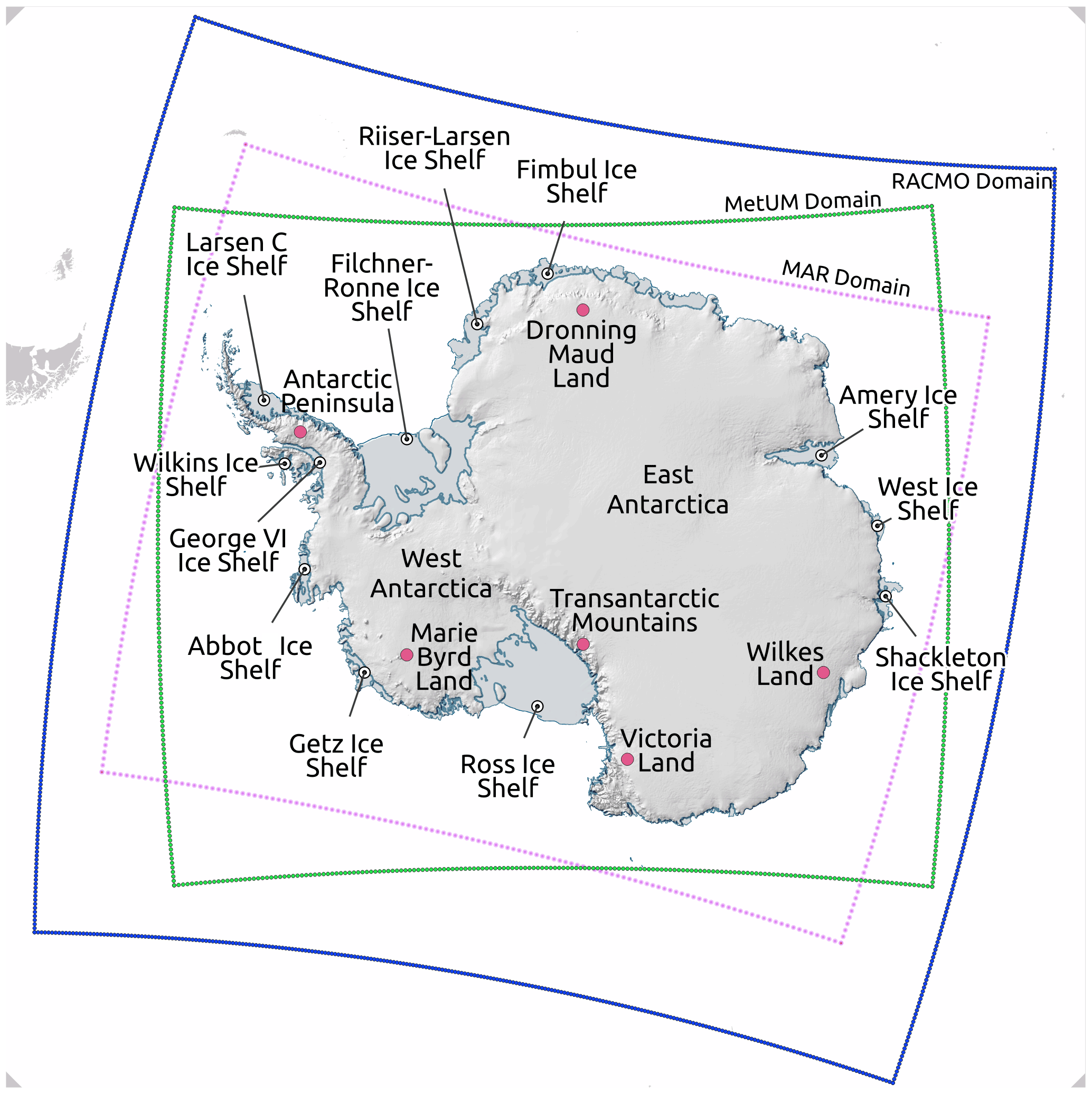
Figure 1 Map of Antarctica with some of the main regions and ice shelves labelled, made using the Quantarctica mapping environment (Matsuoka et al., 2021). The RCM simulation domains for the MetUM (green), RACMO (blue) and MAR (purple) are shown. A 1 km resolution hillshade has been applied from Bedmap2 (Fretwell et al., 2013).

To study annual, seasonal and monthly variability separately, seasonal and trend decomposition using LOESS (STL) (Cleveland et al., 1990) is applied to the time series of each variable at each grid cell. This results in individual trend (T), seasonal (S) and residual (R) components. The decomposition is additive, meaning for each data point (ν)=1 to N, the components are summed to give the original time series (Y) (Eq. 1). The trend component represents the low-frequency–long-timescale pattern of the time series, after filtering out medium- and high-frequency signals including the seasonal component, which captures periodic patterns, and the residual component that explains fluctuations not caused by the long-scale trend or periodicity in the time series.

$$\begin{array}{}\text{(1)}& Y_{\mathit{\nu }}=T_{\mathit{\nu }}+S_{\mathit{\nu }}+R_{\mathit{\nu }}\end{array}$$

Basic time series decomposition involves first approximating the trend component by applying a polynomial fit through the data. Subtracting this component gives the detrended data that are then split into seasonal sub-series (e.g. January, February), and an average of each sub-series gives the seasonal component of the data. Subtracting both the trend and seasonal components then gives the residual component of the series. STL is a more sophisticated procedure that allows options such as robust fitting (where the influence of outliers is limited) and also a time-varying seasonal component. The algorithm is iterative and involves two loops: the outer loop reduces the influence of outliers by assigning weights based on the magnitude of the remainder term; the inner loop involves estimation of the trend and seasonal components through iterative feedback (Cleveland et al., 1990).

The seasonal component is allowed to vary smoothly over the time series, which is done by applying a LOESS (local regression) smoothing to the monthly sub-series with window length n_s. As n_s→∞ the LOESS smoothing becomes equivalent to simply taking the average over the sub-series. The value of n_s is recommended to be greater than 7 (Cleveland et al., 1990). As the value increases, the seasonal component approaches a constant periodic state. In this work 13 is used as this allows potential decadal oscillations in the climate, such as the Pacific Decadal Oscillation (PDO), to be captured in the seasonal component.

The trend component is estimated using LOESS with a window of default size (n_t) given by the smallest odd integer greater than the value in Eq. (2), which for a period (n_p) of 12 months and seasonal smoother (n_s) of 13 gives n_t=21. This means the seasonal component can be thought of as a 12-month periodic signal that is allowed to change gradually over a 13-year period, while the trend component can be thought of as similar to the result of taking a weighted moving average of the deseasonalised time series over a 21-month period. The residual component is then the remaining signal not described by either the smoothly varying seasonal cycle or the long-timescale trend. An example of applying STL decomposition to the time series of snowfall, surface temperature and melt for a grid cell on the Larsen C ice shelf is available in Appendix A.

$$\begin{array}{}\text{(2)}& n_{\mathrm{t}}\ge {\displaystyle \frac{\mathrm{1.5}{n}_{\mathrm{p}}}{\mathrm{1}-\mathrm{1.5}{n}_{\mathrm{s}}^{-\mathrm{1}}}}\end{array}$$

In this paper temporal variability between the ensemble of Antarctic-wide datasets is assessed in several ways, including calculating the Pearson linear correlation coefficient between the outputs for each component of the time series and each variable of interest, quantifying differences in the mean of the time series as well as in the standard deviation of the seasonal and residual components, and calculating the root mean square deviation (RMSD) between the outputs for each variable of interest. Each metric is calculated for every grid cell in the domain, with Antarctic-wide plots showing spatial patterns. Differences in the monthly mean and standard deviation of the components are calculated over the 37-year 1981–2018 period. For snowfall and melt, differences at each grid cell are expressed as a proportion of the respective inter-annual deviations, providing some measure of the relative significance of differences at each location. The impact of systematic differences in snowfall and melt on estimates of ice shelf stability depends not only on absolute magnitudes but also on the relative magnitude against a baseline variance. The inter-annual baseline deviation at each grid cell is approximated as the ensemble average standard deviation in the trend component of the time series. Results presented in spatial maps then show the relative significance of systematic differences and are not simply dominated by the sites with the highest-magnitude snowfall/melt.

4 Results

Variability in the ensemble of Antarctic-wide outputs (Table 1) for the monthly time series of snowfall, near-surface air temperature and melt are quantified across the domain through the evaluation of metrics including the correlation between the outputs, systematic differences in the mean and in the seasonal and residual standard deviations, and the RMSDs between outputs. These metrics, for variability in the time series, are evaluated at each grid cell, and the main results are shown in Sect. 4.1, 4.2 and 4.3. Spatial maps are used to show large- and small-scale patterns in the metrics across the domain. Discussion of the results, including features of variability and the relative importance of contributing factors, is given in Sect. 5.

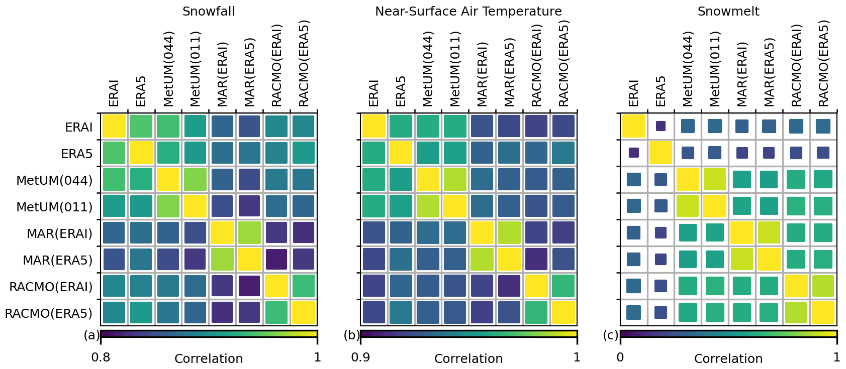
Figure 2 The correlation for snowfall (a), near-surface air temperature (b) and melt (c) between models averaged over the ice sheet. The colour scale relates to the value of correlation, and the scale is adjusted for each plot. The size of each square also relates to the value of correlation, although it is kept constant across the figures, going from 0–1, to make comparisons clear between the different variables.

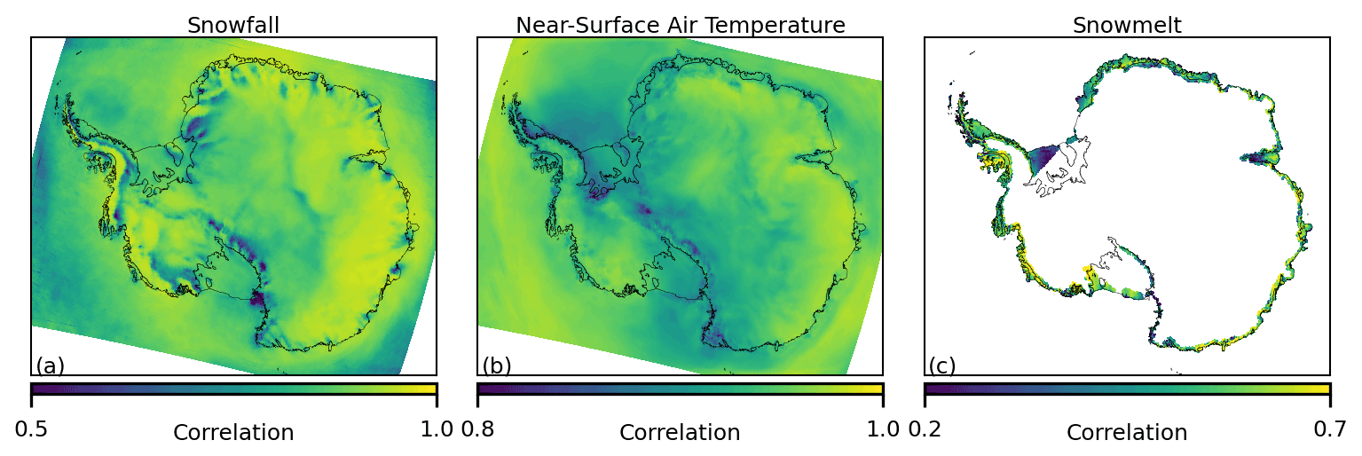
Figure 3 The median correlation by grid cell in the residual component of the monthly time series between the 28 unique model pairs for snowfall (a), near-surface air temperature (b) and melt (c). The colour scale relates to the value of correlation, and the scale/limits are adjusted for each plot.

4.1 Correlation

Results are presented for the correlation in the deseasonalised and detrended residual component of the time series between each of the 28 unique model output pairs. The correlation is computed at every grid cell, and for melt, grid cells where the ensemble 40-year average monthly melt is less than 1 mm water equivalent per month (mm w.e. per month) are masked as these regions only experience sporadic and insignificant-magnitude melt events, essentially equating to numerical noise in the simulations. The average grid-cell correlation across the entire ice sheet is then taken, and the results are given in Fig. 2. High correlation is shown for snowfall (>0.80) and near-surface air temperature (>0.90) across all model pairs, while results for melt show a significant divide between the reanalysis datasets and the RCMs. The correlation for melt between just the RCMs is moderate to high (>0.55) across all pairs, while for the reanalysis datasets the correlation is low (<0.35) for comparisons to all other models, including between ERA-Interim and ERA5. Another key feature includes the comparatively high correlation shown in every variable between simulations of the same RCM but differing resolution/driving data (MetUM(044)–MetUM(011), MAR(ERAI)–MAR(ERA5) and RACMO(ERAI)–RACMO(ERA5)).

A spatial map of the median correlation in the residual component across the 28 unique model output pairs is plotted in Fig. 3. An ice-sheet-only mask is applied for melt using the high-resolution shapefile from Depoorter et al. (2013), which is found to remove the most prominent edge effects caused by comparing high- and low-resolution models for a variable that is dependent on the sea/ice categorisation of the grid cell. In addition, grid cells where the ensemble 40-year average melt is less than 1 mm w.e. per month are again masked. In Fig. 3 the median correlation for near-surface air temperature is shown to be high (>0.8) across the ice sheet, while for snowfall the correlation remains high again across the majority of the ice sheet but is moderate to low over regions such as the Transantarctic Mountains, where the topography varies sharply. For melt, the correlation is moderate over the majority of ice shelves, although is noticeably low over the Ronne ice shelf, the ice shelves bounding Victoria Land and the interior of the Amery ice shelf.

4.2 Mean and standard deviation: magnitude and spatial pattern of differences

The 1981–2018 mean and standard deviation for each component of the monthly time series of the ice sheet total snowfall, average near-surface air temperature and total melt are displayed in Table 2. Results show that even aggregated across the entire ice sheet, significant systematic differences exist between the outputs for each variable. For example, the magnitude of differences in the mean across the ensemble is comparable to the average trend standard deviation, which represents inter-annual variations. One particularly striking feature is the contrast between the low monthly melt of ERA5 (1.1 Gt per month) compared to the high monthly melt of ERA-Interim (15.5 Gt per month) and all RCMs (9.1–14.2 Gt per month). It is noted that the relative magnitudes of standard deviations in each component of the time series depend on the variable and that for temperature and melt the seasonal deviation is dominant, while for snowfall both the seasonal and the residual deviations have similar magnitudes. Another feature is that systematic differences are comparatively low between simulations of the same RCM but differing resolution/driving data (MetUM(044)–MetUM(011), MAR(ERAI)–MAR(ERA5) and RACMO(ERAI)–RACMO(ERA5)) when compared with differences present between the different RCMs.

To understand how systematic differences vary spatially, the 1981–2018 mean and seasonal and residual standard deviations for the monthly time series of each variable are also computed at a 12 km grid-cell level. Since it is found that systematic differences in the mean and standard deviations are most pronounced between different models in the ensemble, results presented in Figs. 4, 5 and 6 are filtered to only include ERA5, MetUM(011), MAR(ERA5) and RACMO(ERA5). Differences for each model are then plotted relative to this reduced ensemble average (model-ensemble avg). Results showing direct comparisons between the same/similar model pairs are given in Figs. B1, B2 and B3 in the Appendix and include differences in the mean and standard deviations between ERA-Interim and ERA5, MetUM(044) and MetUM(011), MAR(ERAI) and MAR(ERA5), and RACMO(ERAI) and RACMO(ERA5). Differences in the standard deviation of the trend component are excluded from grid-cell-level results as it is shown in Table 2 that the relative magnitude against standard deviations in the seasonal and residual components is low. For snowfall and melt, differences at each grid cell are expressed as a proportion of the respective inter-annual deviations, approximated by the ensemble average standard deviation in the trend component.

Table 2 After aggregating across the ice sheet, the mean and standard deviation for each component of the monthly time series for total snowfall, average near-surface air temperature and total melt are given. Values for snowfall and melt are expressed in units of gigatonnes, while values for temperature are expressed in kelvin.

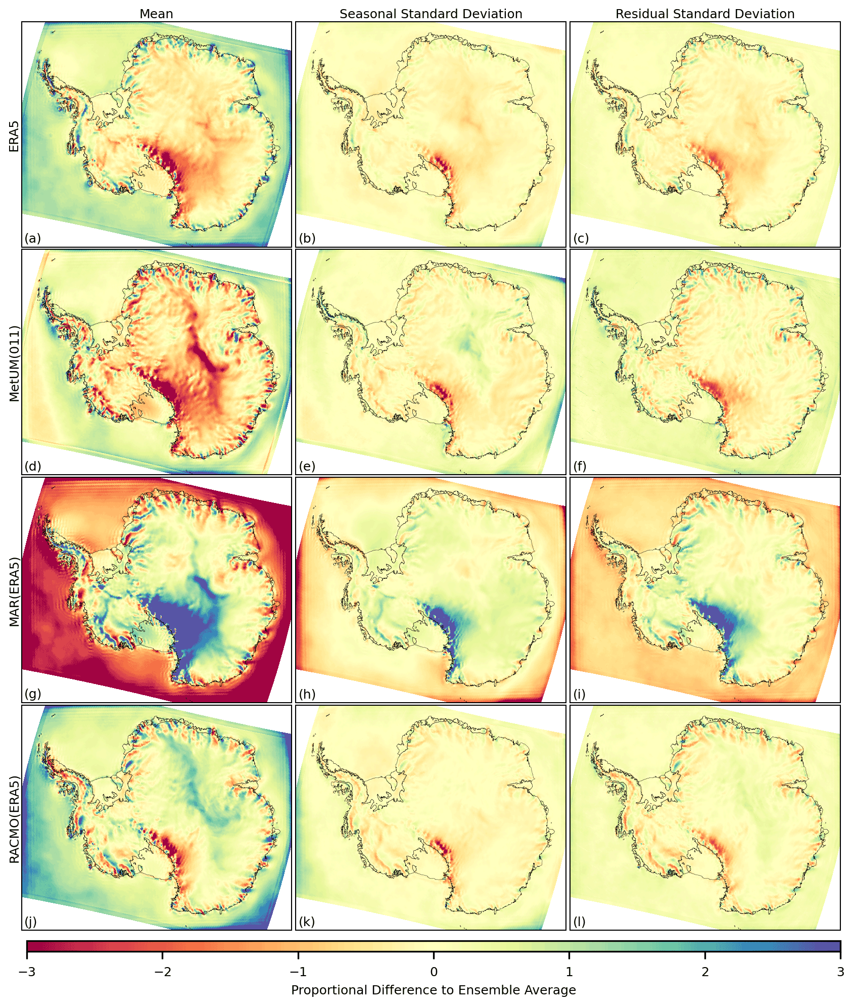
Figure 4 The difference to the ensemble average (model-ensemble avg) for the 1981–2018 time series of snowfall, in the mean (a, d, g, j), the standard deviation of the seasonal component (b, e, h, k) and the standard deviation of the residual component (c, f, i, l). The ensemble includes ERA5 (a–c), MetUM(011) (d–f), MAR(ERA5) (g–i) and RACMO(ERA5) (j–l). Differences at each grid cell are expressed as a proportion of average inter-annual variation and so do not have units.

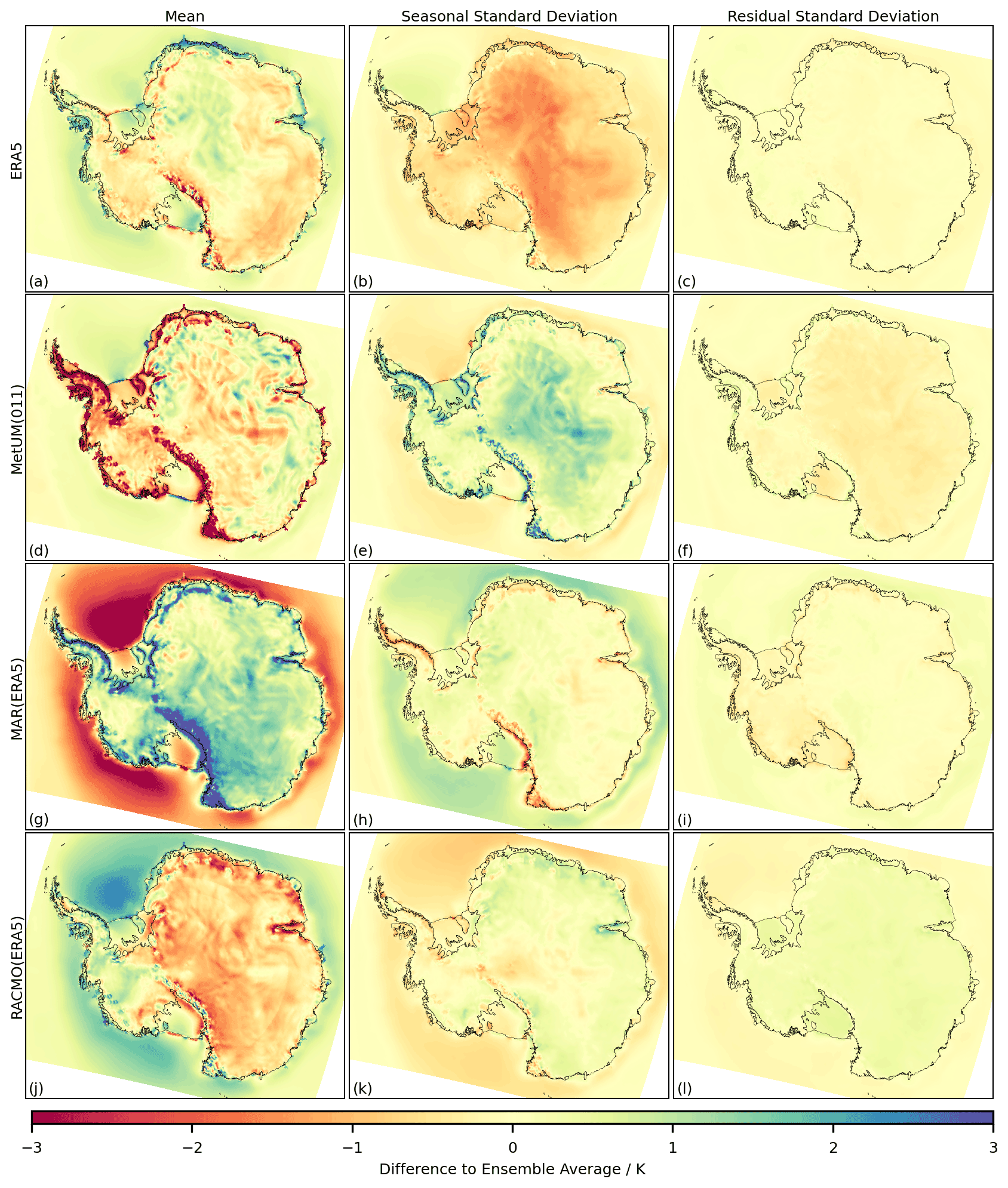
Figure 5 The difference to the ensemble average (model-ensemble avg) for the 1981–2018 time series of near-surface air temperature, in the mean (a, d, g, j), the standard deviation of the seasonal component (b, e, h, k) and the standard deviation of the residual component (c, f, i, l). The ensemble includes ERA5 (a–c), MetUM(011) (d–f), MAR(ERA5) (g–i) and RACMO(ERA5) (j–l).

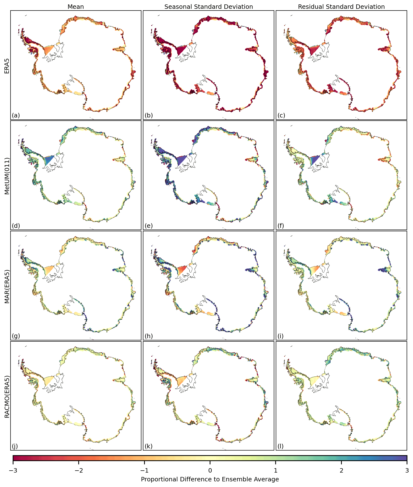
Figure 6 The difference to the ensemble average (model-ensemble avg) for the 1981–2018 time series of melt, in the mean (a, d, g, j), the standard deviation of the seasonal component (b, e, h, k) and the standard deviation of the residual component (c, f, i, l). The ensemble includes ERA5 (a–c), MetUM(011) (d–f), MAR(ERA5) (g–i) and RACMO(ERA5) (j–l). Differences at each grid cell are expressed as a proportion of average inter-annual variation and so do not have units. Grid cells where the ensemble mean average monthly melt is less than 1 mm w.e. per month are masked.

In Fig. 4, it can be seen that for snowfall there exists high-magnitude, spatially coherent, systematic differences over both the ocean and the ice sheet, particularly in the mean of the time series (Fig. 4a, d, g, j), for each model relative to the ensemble average. A specific example is the strong negative difference in the mean snowfall over the ocean and strong positive difference over the majority of the ice sheet shown by MAR (Fig. 4g). In general, the positive/negative sign of the differences in the mean and standard deviations for snowfall over the interior of the ice sheet, over the Transantarctic Mountains and over the oceans show a relatively large spatial correlation length scale. In contrast, near the periphery of the ice sheet, the sign of the differences exhibits a smaller correlation length scale. Regions such as the Antarctic Peninsula exhibit direction-dependent length scales, with a comparatively large length scale in the latitude direction and a comparatively short length scale in the longitude direction. The magnitude of the differences shown over the ice sheet appears greater over sharply varying topography, such as the Transantarctic mountain range and the steep coastal slopes of the ice sheet. An exception to this is high-magnitude differences also shown in the mean component over the comparatively flat region of the interior of East Antarctica for the MetUM(011) and MAR(ERA5) (Fig. 4d, g).

It can be seen that for snowfall the difference present in the mean of the time series has a similar spatial signature and sign to the difference in the standard deviation of the seasonal and residual components (e.g. Fig. 4g–i). Exceptions to this include for example the difference in snowfall from the MetUM(011) relative to the ensemble in the interior of East Antarctica, where despite having a lower mean snowfall, the standard deviation in the seasonal component is greater than the average of the ensemble (Fig. 4d and e).

As with snowfall, there exist significant differences over both the ocean and the land for near-surface air temperature between the models, again particularly in the mean of the time series (Fig. 5). For example, MAR shows a significant positive difference in the mean of the time series over the majority of the ice sheet (Fig. 5g) and a significant negative difference over the majority of the surrounding ocean. The magnitude of differences shown over the ice sheet again appears greater over regions of steep topography, particularly for the MetUM(011) and MAR(ERA5) outputs (Fig. 5d, g). The spatial patterns of differences in near-surface air temperature differ in shape compared to those present for snowfall. In particular, near the edge of the ice sheet there are fewer positive-to-negative fluctuations with changing longitude and instead the patterns are more parallel to the coastline (Fig. 5d, g). While there are similar spatial patterns between the mean temperature difference and the seasonal standard deviation difference (as for Fig. 4), the sign of the differences in Fig. 5 is in general shown to change, for example over the majority of the ice sheet in Fig. 5d compared with Fig. 5e. In Fig. A1e in the Appendix, which gives the temperature profiles from each simulation over an example grid cell on the Larsen C ice shelf, a colder mean temperature is shown to be the result of similar summer temperatures with more severe winter temperatures.

A land-only mask has been applied for melt in Fig. 6 as well as a filter masking any grid cells where the ensemble mean average monthly melt is less than 1 mm w.e. per month. This limits discussion of the patterns in differences in the mean and standard deviations to the peripheral areas, which are predominantly ice shelves. The magnitude of the differences present is, as for snowfall, significant relative to the inter-annual variability in melt at each grid cell. Unlike for snowfall and near-surface temperature, the relative magnitude of differences across the ensemble in the standard deviation of both the seasonal and the residual components of the time series is greater than differences present in the mean of the time series. It is noted that for melt, which occurs primarily over just the summer months, greater values of standard deviation in the seasonal component are expected to represent both/either higher magnitudes over peak months and/or a prolonged melt season. As with near-surface temperature and snowfall there are patterns of both short and long spatial length scales. An example of a relatively localised spatial pattern is that of the strong positive difference shown by MAR over the interior of the Amery ice shelf in the mean of the time series, as well as in the standard deviation of the seasonal and residual components. An example of a large-scale pattern is that ERA5 shows a considerable negative difference in the mean and standard deviations of melt over the majority of ice shelves.

4.3 RMSD

The RMSD of the monthly time series is evaluated at each grid cell for each of the 28 unique output pairs of the ensemble. For snowfall and melt, the metric is scaled at each grid cell by the ensemble average inter-annual standard deviation, described here as the proportional RMSD value. The average is then taken across the ice sheet for each variable, and results are given in Fig. 7a–c. The average RMSD across the ice sheet provides a measure of the average deviation between the time series of two model outputs at each grid cell, while the average proportional RMSD gives a measure of the average relative magnitude of deviations with respect to inter-annual variability. In addition, the percentage reduction in RMSD/proportional RMSD is evaluated after adjusting the mean as well as the seasonal and residual standard deviations at each grid cell for every model output to that of the ensemble average. The average percentage reduction is then taken across the ice sheet for each variable, and results are given in Fig. 7d–f. This percentage reduction gives a measure of what proportion of the deviations between the time series are the result of systematic differences in the mean as well as in the seasonal and monthly fluctuations.

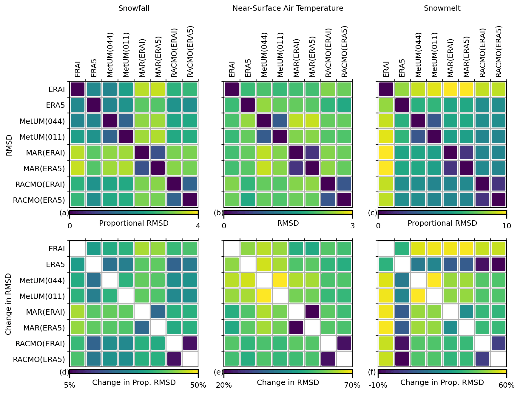
Figure 7 The RMSD/proportional RMSD for snowfall (a), near-surface air temperature (b) and melt (c) between models averaged over the ice sheet. It is noted for melt that grid cells where the ensemble average is less than 1 mm w.e. per month are excluded. After adjusting the mean as well as the seasonal and residual standard deviations of all outputs to the ensemble average, the percentage reduction in RMSD/proportional RMSD is plotted for snowfall (d), near-surface air temperature (e) and melt (f).

From Fig. 7 it can be seen the average values for the RMSD/proportional RMSD are significant for all variables, with upper thresholds of 3 K for near-surface air temperature and proportional values of 4 for snowfall and 10 for melt. Values are comparatively low between simulations of the same RCM but differing resolution/driving data (MetUM(044)–MetUM(011), MAR(ERAI)–MAR(ERA5) and RACMO(ERAI)–RACMO(ERA5)) when compared with differences present between the different RCMs. For melt, ERA-Interim has noticeably higher values of proportional RMSD compared to the other models, while for snowfall and temperature differences are less pronounced, but the two simulations from MAR show higher average proportional RMSD for snowfall compared with the other models.

The percentage change in RMSD/proportional RMSD after adjusting for equal means as well as seasonal and residual standard deviations is significant for all variables, as shown in Fig. 7. Upper thresholds of the percentage reduction are 50 %, 70 % and 60 % for snowfall, near-surface air temperature and melt respectively. For melt, the most significant reductions are for ERA-Interim, while ERA5 shows the least significant reductions with proportional RMSD actually increasing between ERA5 and the RACMO products. Across the variables it can be seen that the percentage reduction in RMSD between the high-resolution–low-resolution MetUM simulation pairs is of greater magnitude than reductions between the two ERA-Interim-driven–ERA5-driven RACMO pairs and two ERA-Interim-driven–ERA5-driven MAR pairs.

5 Discussion

The results presented in this paper show that for all variables studied, when considered across the entire ice sheet, the outputs that came from the same model (MetUM(011/044), MAR(ERAI/ERA5), RACMO(ERAI/ERA5)) exhibit the highest correlations in the time series as well as the smallest systematic differences and RMSDs. This is despite significant differences in resolution between the MetUM runs, which span the highest- and lowest-resolution RCM simulations made available from the Antarctic CORDEX project, as well as significant differences in the driving data for the two MAR and RACMO runs. Note that, although ERA5 is an update to ERA-Interim, the results in Table 2 and in Appendix B show that the magnitude of systematic differences in the mean and standard deviations between the reanalysis datasets is of similar magnitude to or greater magnitude than that of differences between different RCM outputs (Figs. 4, 5 and 6). Updates in the model physics and assimilation techniques used by ERA5 (Hersbach et al., 2020) compared to ERA-Interim are hypothesised to be the primary reason for large-scale differences in snowfall and near-surface air temperature identified between the reanalysis outputs. While EAR-Interim and ERA5 exhibit large differences in their DEMs (Fig. C1), it is argued in Sect. 5.1 that differences in DEMs are not primary contributors to systematic differences in the models' output. The particularly significant difference (over an order of magnitude) for ice-sheet-wide melt between ERA-Interim (15.5 Gt) and ERA5 (1.1 Gt) is hypothesised to be primarily due to an updated surface scheme (HTESSEL) used in ERA5 that allows runoff (Balsamo et al., 2009).

Results therefore suggest that differing resolution and driving data are not primary contributors to large-scale spatial variability across the ensemble. Similarity in the spatial and temporal patterns between Antarctic-wide outputs of the same RCM with different driving data agrees with findings from Agosta et al. (2019), where outputs from MAR are compared with differing reanalysis driving data from ERA-Interim, JRA-55 and MERRA-2. Similarity in results aggregated over the ice sheet (Table 2) between Antarctic-wide outputs of the same RCM with different driving data agrees with findings from Mottram et al. (2021) where SMB for two simulations of differing resolution (12 and 50 km) for the RCM HIRHAM5 is compared against other RCMs. At finer, more localised scales differing resolution is shown to create significant differences in the mean as well as the seasonal and residual standard deviations for the monthly time series of each variable; see Figs. B1, B2 and B3d–f in the Appendix, which show direct comparisons between the high- and low-resolution MetUM simulations.

The magnitude of differences in snowfall and near-surface air temperature due to resolution is greatest over regions of sharply varying topography, such as the Transantarctic Mountains, the coastal slopes of the ice sheet and the Antarctic Peninsula. The representation of atmospheric processes occurring over mountainous regions including föhn winds that occur over the Antarctic Peninsula and katabatic winds occurring over the coastal slopes of East Antarctica is known to be resolution dependent (Orr et al., 2014, 2021; Heinemann and Zentek, 2021). Föhn and katabatic winds have been shown to impact climate over ice shelves, which are often in the close vicinity of steep terrain, and are an important driver of surface melt (Bromwich, 1989; Cape et al., 2015; Lenaerts et al., 2017; Datta et al., 2019; Elvidge et al., 2020). In Fig. B2d the difference in the mean near-surface air temperature, due to resolution, extends over ice shelves such as the interior of the Amery ice shelf, which is a well-known katabatic wind confluence zone (Parish and Bromwich, 2007). Despite this influence of resolution on the climatology over ice shelves, greater systematic differences in melt shown in Fig. 6 compared with Fig. B3d–f indicate the potentially more significant importance of differences in surface schemes across the particular ensemble of RCMs studied. It is expected that even at 12 km resolution, climatically important terrain-induced atmospheric processes, such as föhn/katabatic winds, are not being realistically resolved, as is shown in Orr et al. (2021), where output from the MetUM RCM at 4, 1.5 and 0.5 km during a föhn wind event on the Larsen C ice shelf shows no obvious convergence towards observations during the event.

The same-model RCM simulations in the ensemble, as well as having identical model physics, parametrisation and tuning, also share factors such as the domain specification, ice mask applied, digital elevation model and boundary conditions. The relative contribution of these additional factors is explored in Sect. 5.1, and from this it is argued that the joint influence of choices in model physics, parametrisation and tuning is the primary factor influencing large-scale variability across the ensemble. The impact of parameter tuning is discussed in Gallée and Gorodetskaya (2008), where it is shown that adjusting the relative contribution of snow particles compared to ice particles in MAR's radiative scheme has a significant impact on near-surface air temperature. A higher relative contribution of snow particles leads to greater flux in long-wavelength downward radiation. In addition to exploring the relative contribution of different factors to the large spatial-scale variability in the ensemble, in Sect. 5.2 specific features of the variability that are mentioned in Sect. 4 are discussed and the nature of variability for different variables, regions and timescales is examined.

5.1 Contribution to variability from the choice of domain, ice mask, boundary conditions and DEM

The exact spatial domains differ between the RCM simulations as shown in Fig. 1. However, the spatial domain for all RCM simulations examined is Antarctic-wide and domain boundaries all exist over the ocean, implying there should be no strong local forcing at any of the boundaries. The effect of increasing domain size over the ocean on the output of simulations from MAR over the Greenland ice sheet has previously been studied and has been found to not significantly impact results over the ice sheet (Franco et al., 2012). In general, the domain size should be great enough such that the buffer zone, in which boundary conditions are applied, does not intersect the region of interest, which in this case is the Antarctic ice sheet. It is found that for the MetUM(044) run, the buffer zone intersects some areas of the periphery of the ice sheet, shown clearly in Fig. B1d. Despite this, it can be seen that effects are localised to the buffer zone boundary and that even for the regions of the ice sheet that intersect this, the relative impact on systematic differences appears less significant than other factors explored. Overall it is assumed that, for the ensemble of RCM simulations studied, differences in the domains do not have a significant effect on the model output for surface climatology over the ice sheet.

As well as having differences in the outer domain boundaries, the different models also have slight differences in the specified boundaries of the ice sheet due to different coordinates and ice masks used. This creates edge effects at the periphery of the ice sheet, which are particularly noticeable for melt in for example Fig. 5d at the edges of the Ronne–Filchner and Ross ice shelves. It is shown in Mottram et al. (2021) and Hansen et al. (2022) that these edge effects, due to inconsistent ice masks, can have a significant impact on the total estimated SMB over the ice sheet. In this paper, although ice-sheet-wide totals are computed (Table 2), the focus is primarily on evaluating variability in the time series at each 12 km grid cell after regridding products to a common high-resolution grid. Results for spatial maps of differences for melt are masked using an ice-sheet-only mask from Depoorter et al. (2013), which is found to exclude the most significant edge effects from areas where low-resolution models overestimate the extent of the ice sheet after regridding. The same mask is applied before calculating average correlations and RMSDs also reducing the impact of edge effects. Results presented and discussed here, particularly regarding large-scale spatial patterns, are therefore assumed to not be significantly impacted by the different ice masks used in the ensemble of simulations.

Another important consideration when comparing RCM simulations is how the method of applying boundary conditions varies across the ensemble. In particular, although all RCMs examined are nudged at the boundaries within buffer zones, MAR and RACMO also use spectral nudging that constrains the large-scale circulation in the interior of the domain, while the MetUM instead uses a re-initialisation procedure. Spectral nudging involves applying the relaxation technique throughout the interior of the domain to the long-wavelength components of the climate model fields (von Storch et al., 2000). This constrains the large-scale climatology of the RCM output to that of the driving data while allowing added value by the RCM in the small-scale features. The same is aimed to be achieved with the re-initialisation of the MetUM throughout the domain every 12 h, as discussed in Sect. 2.4. The fact that systematic differences between the MetUM, MAR and RACMO are all of significant and comparable magnitude (Figs. 4g and j, 5g and j, and 6g and j), despite MAR and RACMO sharing the technique of spectral nudging, suggests that differences between the specific approaches of applying large-scale constraints within the ensemble of RCMs studied are not one of the main features contributing to variability in the mean and the seasonal and residual standard deviations of snowfall, near-surface air temperature and melt. It is noted, however, that in general the MetUM simulations, rather than the MAR and RACMO simulations, show slightly higher correlation to the reanalysis driving data across the ice sheet for the monthly time series of snowfall and surface temperature (Fig. 2), indicating that the re-initialisation procedure potentially constrains the output across the ice sheet more than spectral nudging.

The differences between DEMs used across the ensemble are plotted in Fig. C1 in the Appendix. The elevation profiles can be split into three main groups: the coarse elevation profile of ERA-Interim (Fig. C1a); the elevation profiles of ERA5 and the MetUM high- and low-resolution runs (Fig. C1b, c, d); and the elevation profiles of MAR and RACMO (Fig. C1e, f). Differences in the DEMs do not mirror the systematic differences shown in Sect. 4.2. For example, while MAR and RACMO share comparatively similar DEMs, the models do not share similar patterns in systematic differences (Figs. B1, B2 and B3). This indicates differences in the DEMs are not primary contributors to systematic differences in the models output, which is further supported by results displayed in Fig. C2, where weak linear correlation is found between differences in elevation and differences in mean near-surface air temperature.

In this section, features including the domain specification, ice mask applied, digital elevation model and boundary conditions applied are argued to not be the primary contributors responsible for the large-scale systematic differences within the ensemble of model outputs. This result, in addition to the previously discussed secondary contributions of resolution and driving data towards large-scale differences, by way of elimination indicates that the joint influence of choices in model physics, parametrisation and tuning is the primary factor influencing large-scale systematic differences across the ensemble.

5.2 Specific features of the variability

Specific features in the variability, identified and mentioned in Sect. 4, are discussed here. In Sect. 4.1 it is mentioned that for melt there is a clear divide in the average correlation in the residual component of the time series between reanalysis datasets compared with RCMs (Fig. 2). That is the correlations between different RCMs are greater than between reanalysis datasets and RCM outputs. This is not the case for snowfall and near-surface air temperature, suggesting the divide in correlation for melt is primarily due to differences in the sophistication and polar-specific tuning of the surface schemes used for the RCM simulations and the global reanalysis products. It is shown in Hansen et al. (2021) that the sub-surface scheme and the handling of layers within the scheme can have a significant impact on melt.

In Sect. 4.1 it is also shown that, particularly for snowfall and melt, the median correlation between the outputs is strongly dependent on the specific region and topography. For melt, three regions are highlighted that show low correlation including the Ronne ice shelf, the ice shelves bounding Victoria Land and the interior of the Amery ice shelf. In the case of the Ronne ice shelf, the low correlation in melt is due to relatively low average melt occurring over the region, so fluctuations away from no melt are small and erratic. Low correlation over ice shelves bounding Victoria Land is expected to be caused by a combination of the ice shelves' fine scale and the sharply varying topography in the region, making the climatology around them difficult to resolve with the resolution available in the climate models. Finally, the pattern of low correlation around regions such as the interior of the Amery ice shelf is likely the result of atmospheric processes difficult to represent fully in the models; for example, katabatic winds, driven by gravity, flowing from the interior of the ice sheet to the exterior down elevation channels have a significant impact on the climate on the Amery ice shelf, particularly near the grounding line (Lenaerts et al., 2017).

As with for correlation, the systematic differences shown between the outputs in the ensemble vary depending on the region and topography; see Sect. 4.2. This is true at large and small spatial scales and for all variables. An example of a dependency at a large scale is in Fig. 4g, where MAR shows a significant positive difference in the 40-year mean monthly snowfall relative to the other outputs over the majority of the ice sheet and a significant negative difference over the majority of the surrounding ocean. In the case of MAR this is hypothesised to be due to a couple of reasons: MAR is forced at the boundaries by humidity and needs time to transform this into precipitation; MAR allows precipitation to be advected through the atmospheric layers until reaching the surface. The advection of precipitation in MAR through each atmospheric layer, in comparison to the instantaneous depositing of precipitation by RACMO, leads to increased snowfall towards the interior of the ice sheet, previously identified in Agosta et al. (2019).

In Sect. 4.3 the RMSD between each model pair, calculated at each grid cell and then averaged across the ice sheet, is presented. This metric of average deviation is dependent on the temporal correlation and presence of systematic differences between the outputs. High values of proportional RMSD for melt, shown in Fig. 7, are the result of relatively low temporal correlations between models as well as relatively high systematic differences. It is noted that for melt, despite there being a clear divide in temporal correlations between reanalysis datasets and RCMs (Fig. 2), the RMSD between ERA5 and the RCMs is of comparable magnitude to values between the RCMs. This is due to particularly low values of total melt exhibited from ERA5 (Table 2) and resulting low-magnitude fluctuations in melt. The percentage change in RMSD, after adjusting the mean as well as the seasonal and residual standard deviations of all outputs to the ensemble average, further supports this as it can be seen for melt that ERA5 exhibits the smallest reduction in RMSD after adjustments (Fig. 7). The converse of the above argument is true for ERA-Interim, which shows particularly high values of total melt and so particularly significant values of RMSD and of percentage reductions after adjusting the mean as well as the seasonal and residual standard deviations. Differences in the model outputs for melt across Antarctica remain significant with respect to inter-annual deviations even after adjusting for systematic differences in the mean and standard deviation of the seasonal and residual components of the time series, indicating the importance of improving surface schemes across the models.

6 Conclusions

The spatial nature and magnitude of variability present in an ensemble of current, state-of-the-art Antarctic-wide RCM outputs and global reanalysis datasets are examined for snowfall, near-surface air temperature and melt. This is done at a 12 km grid level, rather than across elevation bins, which reveals significant spatial patterns in correlation and systematic differences in the mean as well as the seasonal and residual standard deviation. Time series decomposition is used to split comparisons across an approximately inter-annual trend component, a periodic seasonal component and a monthly residual component, which is useful for impact assessments where knowledge of variability in the climate data across different timescales and climate drivers is needed.

It is found that the RCM outputs and reanalysis datasets show high correlation for the monthly time series of snowfall and surface temperature across the majority of Antarctica and the bounding Southern Ocean. Despite this, there exist significant differences, with respect to both magnitude and spatial scale, in the mean as well as the seasonal and residual standard deviations of the time series. In addition, high RMSD between the outputs is found for all variables and is particularly significant for melt with respect to the proportional values relative to annual fluctuations. The primary sources of large-scale, systematic differences between the simulations, for all variables and components, are identified as deriving from differences in the model dynamical core, the surface scheme, and the parametrisation and tuning. Differences in driving data, resolution, domains, ice masks, DEMs and boundary conditions are identified as having a secondary contribution. On local, fine spatial scales the relative contribution from different factors is more complex and differences in for example resolution are shown to have a more significant impact.

The variability in snowfall, near-surface air temperature and melt shown is expected to introduce significant uncertainty in estimates of the ice shelf stability with regard to collapse events, which as discussed may have an important contribution to future SLR estimates. It is suggested that the magnitude and scale of systematic differences across the ensemble preclude the direct use and interpretation of individual outputs in impact assessments regarding ice shelf collapse. Results show that removing systematic differences in the ensemble of outputs significantly reduces the average RMSD. Therefore, as concluded in Mottram et al. (2021), it is important on observational campaigns to correct for systematic differences. Improved coverage and quality of observations will provide greater constraints with which to both tune and update the model physics and parametrisations, as well as to use and reduce uncertainties in post-processing bias correction. In addition, further development of RCMs, with particular focus on improvements to the performance of surface schemes over regions of high melt, is needed to reduce uncertainties around collapse events and future SLR. Finally, it is suggested that further development is needed of sophisticated techniques for bias correction that are compatible with sparse observations and make use of factors such as the spatial distribution of variability identified in this paper.

Appendix A: STL decomposition

Figure A1 shows an example of applying STL decomposition to the time series of snowfall, surface temperature and melt for a grid cell on the Larsen C ice shelf. The decomposition has been applied to each of the eight model outputs examined in this paper. The trend, seasonal and residual components are shown next to the original time series. Decomposing the time series into these components allows some features to be extracted. For example, in the case of snowfall and surface temperature, the models all show high correlation in the inter-annual trend, although there exists a significant systematic difference in the mean between the models. Similarly, for snowfall and surface temperature there is high correlation in the residual term between the models but there is a systematic difference between the models in the standard deviation of that component. In the case of melt, the correlation is more moderate for the trend and residual components, meaning systematic differences are less obvious. The seasonal and residual components in STL decomposition are defined to have an approximately zero mean.

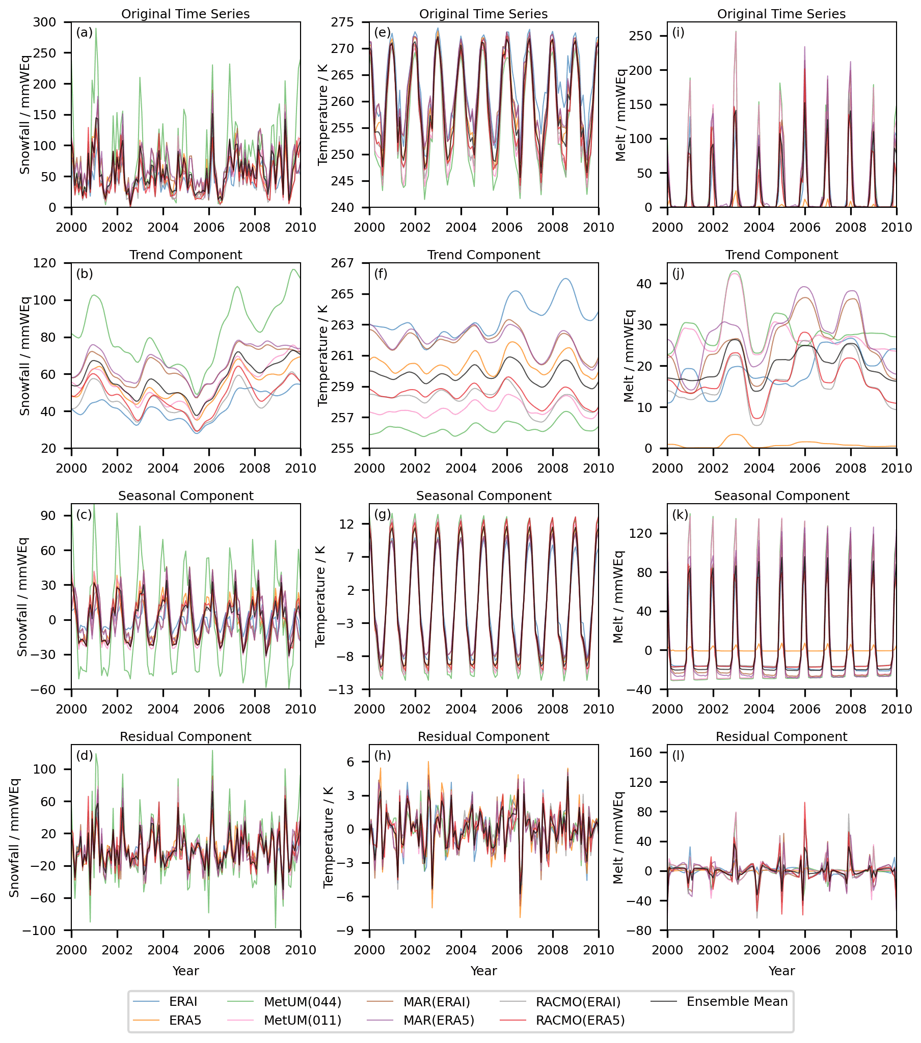
Figure A1 An example of STL decomposition applied to the monthly time series of snowfall (a–d), surface temperature (e–h) and melt (i–l) for a grid cell near the grounding line on the Larsen C ice shelf. The original time series for the years 2000–2010 are shown (a, e, i), as are the trend (b, f, j), seasonal (c, g, k) and residual (d, h, l) decompositions. The model is additive, meaning the sum of trend, seasonal and residual components returns the original time series. Parameter values are n_s=13 and n_t=21.

Appendix B: Same-core-model differences

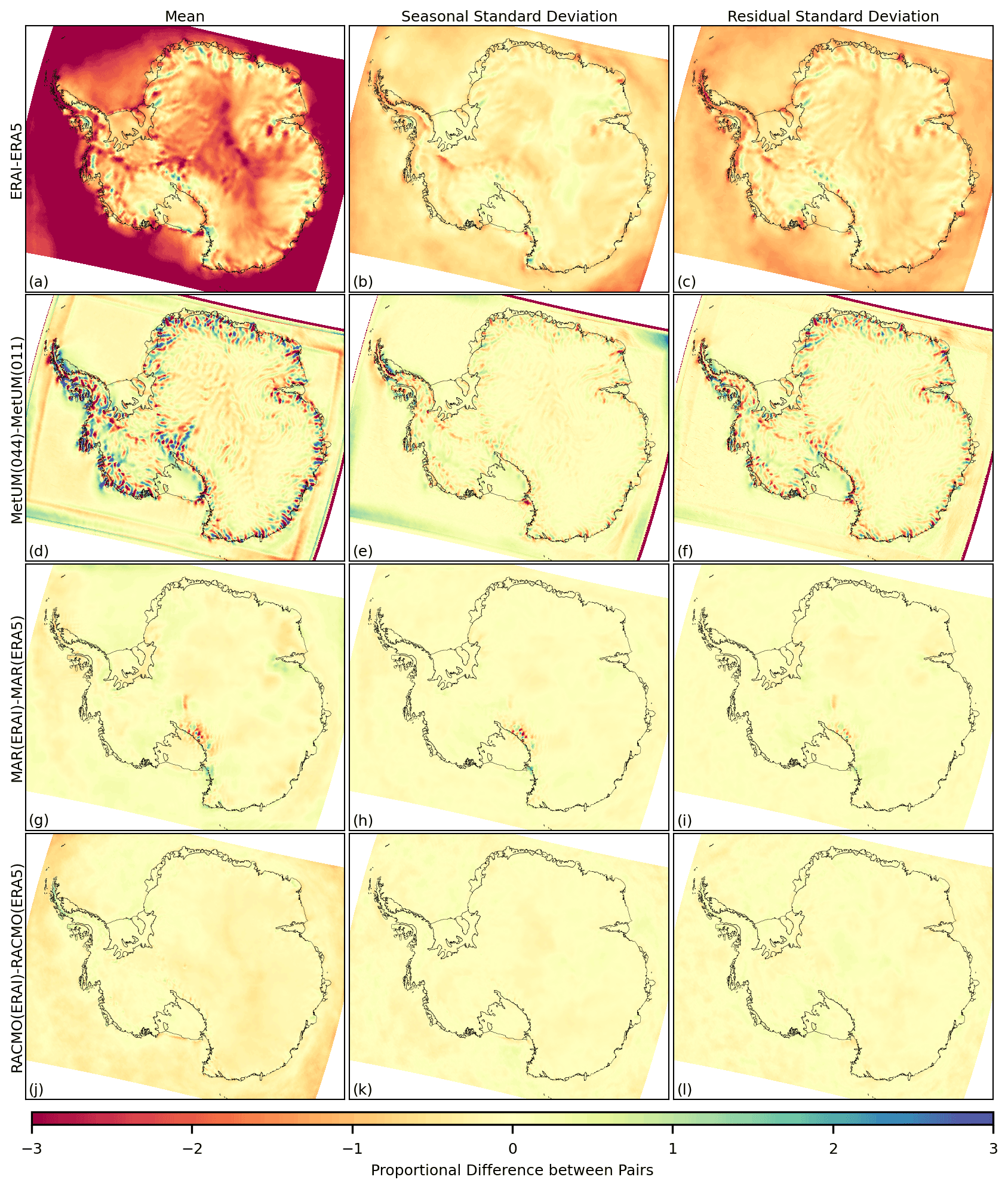
Figure B1 The difference for the 1981–2018 time series of snowfall, in the mean (a, d, g, j), the standard deviation of the seasonal component (b, e, h, k) and the standard deviation of the residual component (c, f, i, l) between the following pairs of outputs: ERA-Interim relative to ERA5 (a–c), MetUM(044) relative to MetUM(011) (d–f), MAR(ERAI) relative to MAR(ERA5) (g–i) and RACMO(ERAI) relative to RACMO(ERA5) (j–l). Differences at each grid cell are expressed as a proportion of average inter-annual variation and so do not have units.

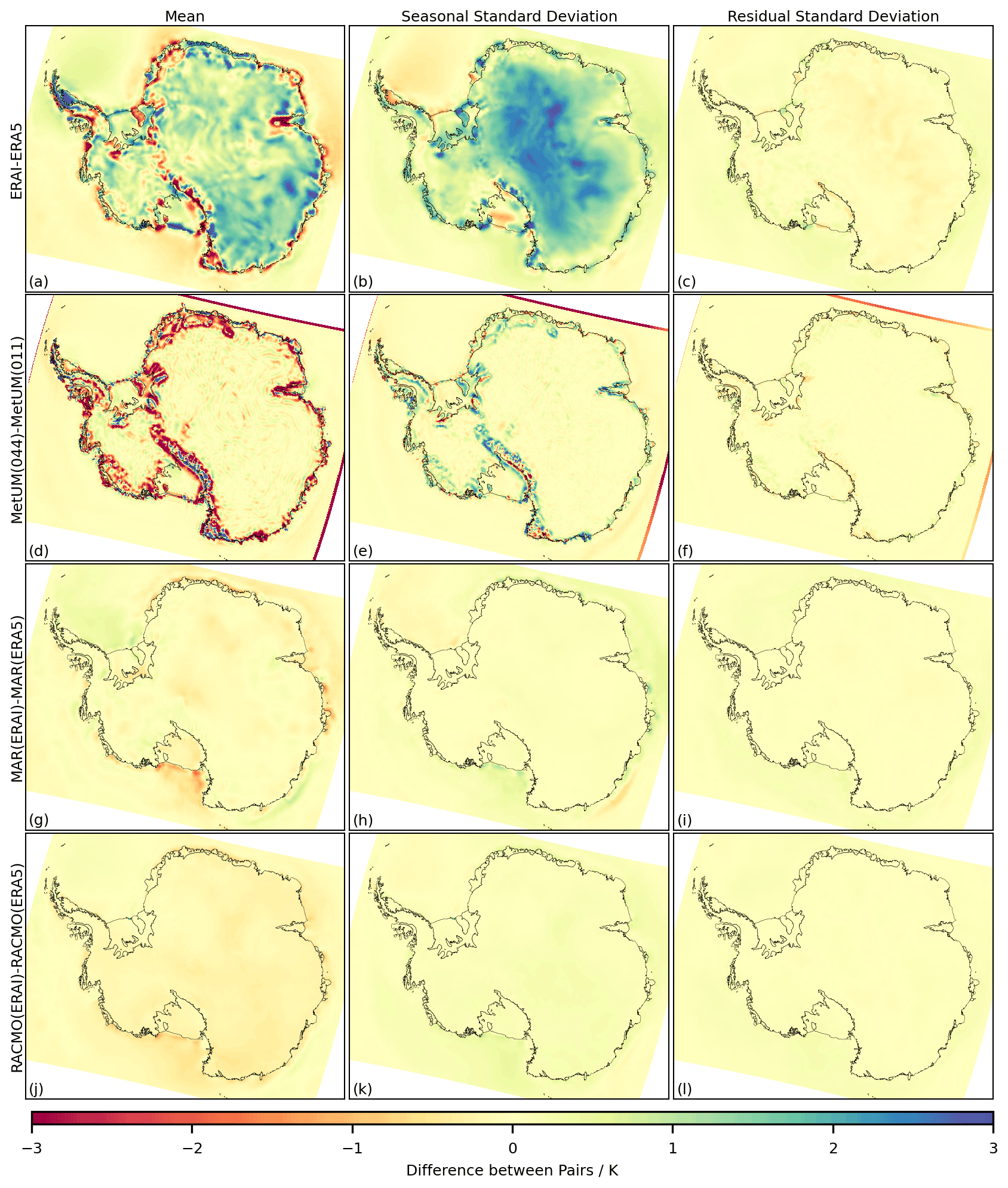
Figure B2 The difference for the 1981–2018 time series of near-surface air temperature, in the mean (a, d, g, j), the standard deviation of the seasonal component (b, e, h, k) and the standard deviation of the residual component (c, f, i, l) between the following pairs of outputs: ERA-Interim relative to ERA5 (a–c), MetUM(044) relative to MetUM(011) (d–f), MAR(ERAI) relative to MAR(ERA5) (g–i) and RACMO(ERAI) relative to RACMO(ERA5) (j–l).

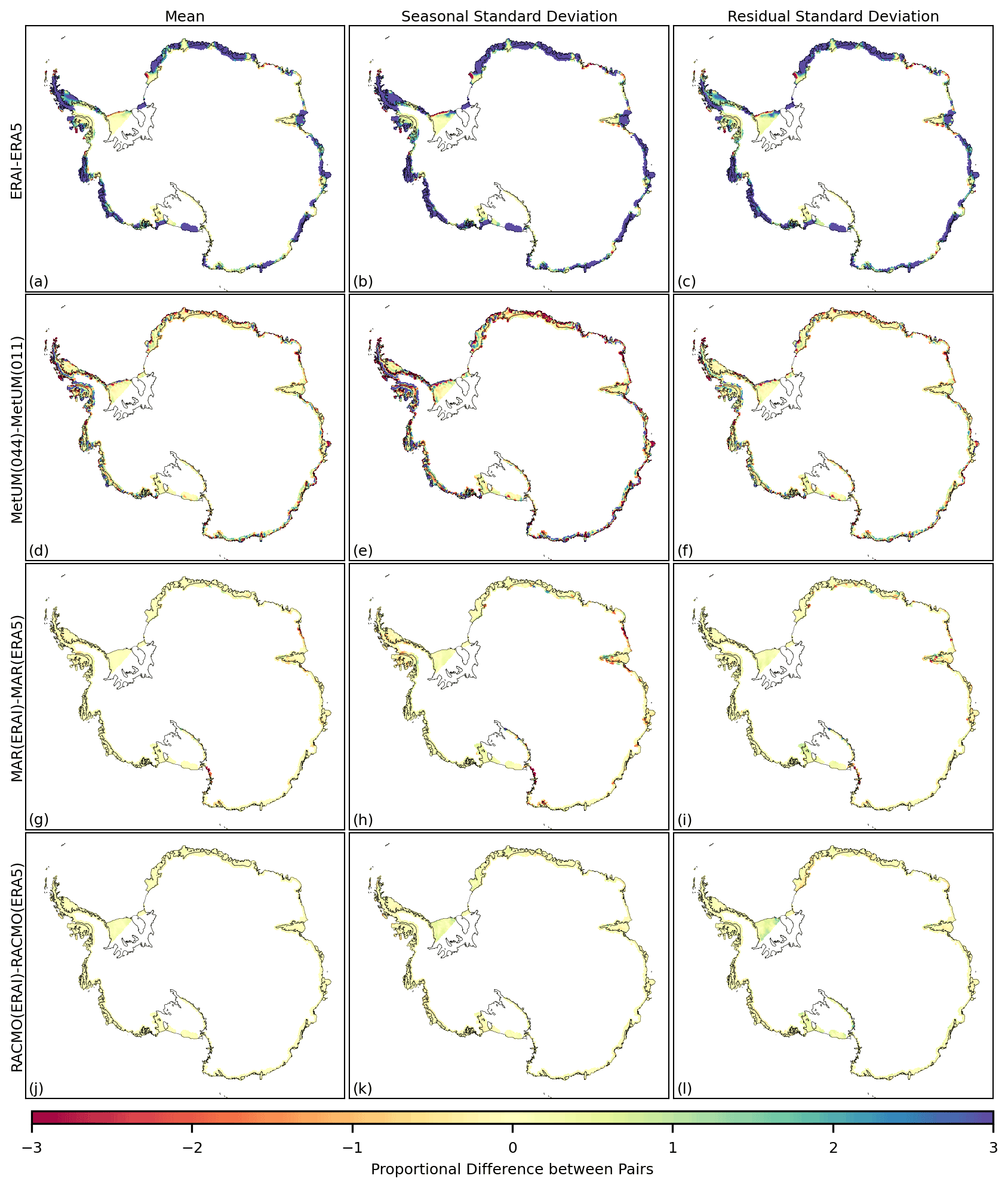
Figure B3 The difference for the 1981–2018 time series of melt, in the mean (a, d, g, j), the standard deviation of the seasonal component (b, e, h, k) and the standard deviation of the residual component (c, f, i, l) between the following pairs of outputs: ERA-Interim relative to ERA5 (a–c), MetUM(044) relative to MetUM(011) (d–f), MAR(ERAI) relative to MAR(ERA5) (g–i) and RACMO(ERAI) relative to RACMO(ERA5) (j–l). Differences at each grid cell are expressed as a proportion of average inter-annual variation and so do not have units. Grid cells where the ensemble mean average monthly melt is less than 1 mm w.e. per month are masked.

Appendix C: DEM differences

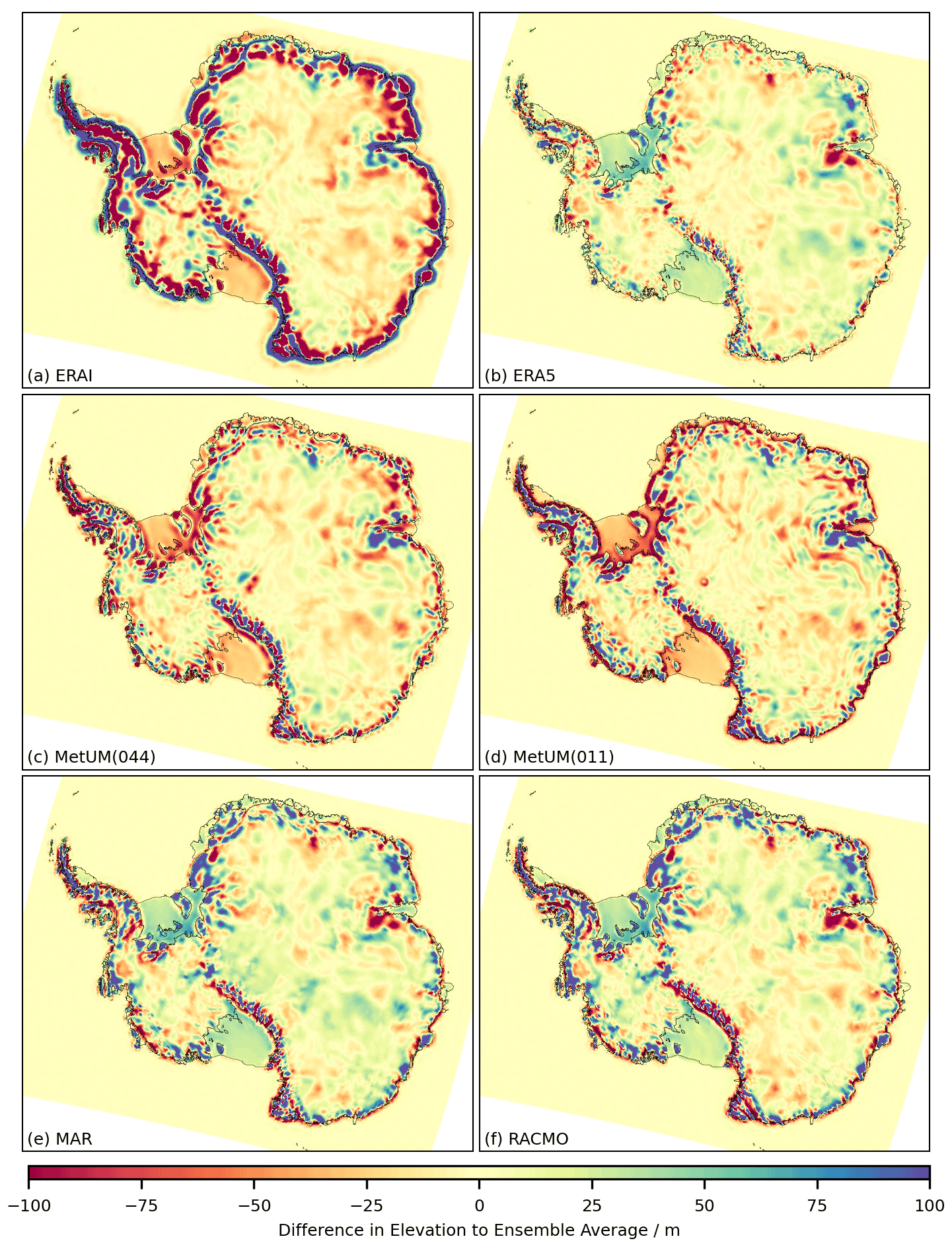
Figure C1 The difference in the DEM used by each climate model relative to the ensemble average is plotted: (a) ERA-Interim, (b) ERA5, (c) MetUM(044), (d) MetUM(011), (e) MAR and (f) RACMO. The DEMs are regridded onto the MetUM(011) 12.5 km² grid for comparison. Units are metres of elevation difference.

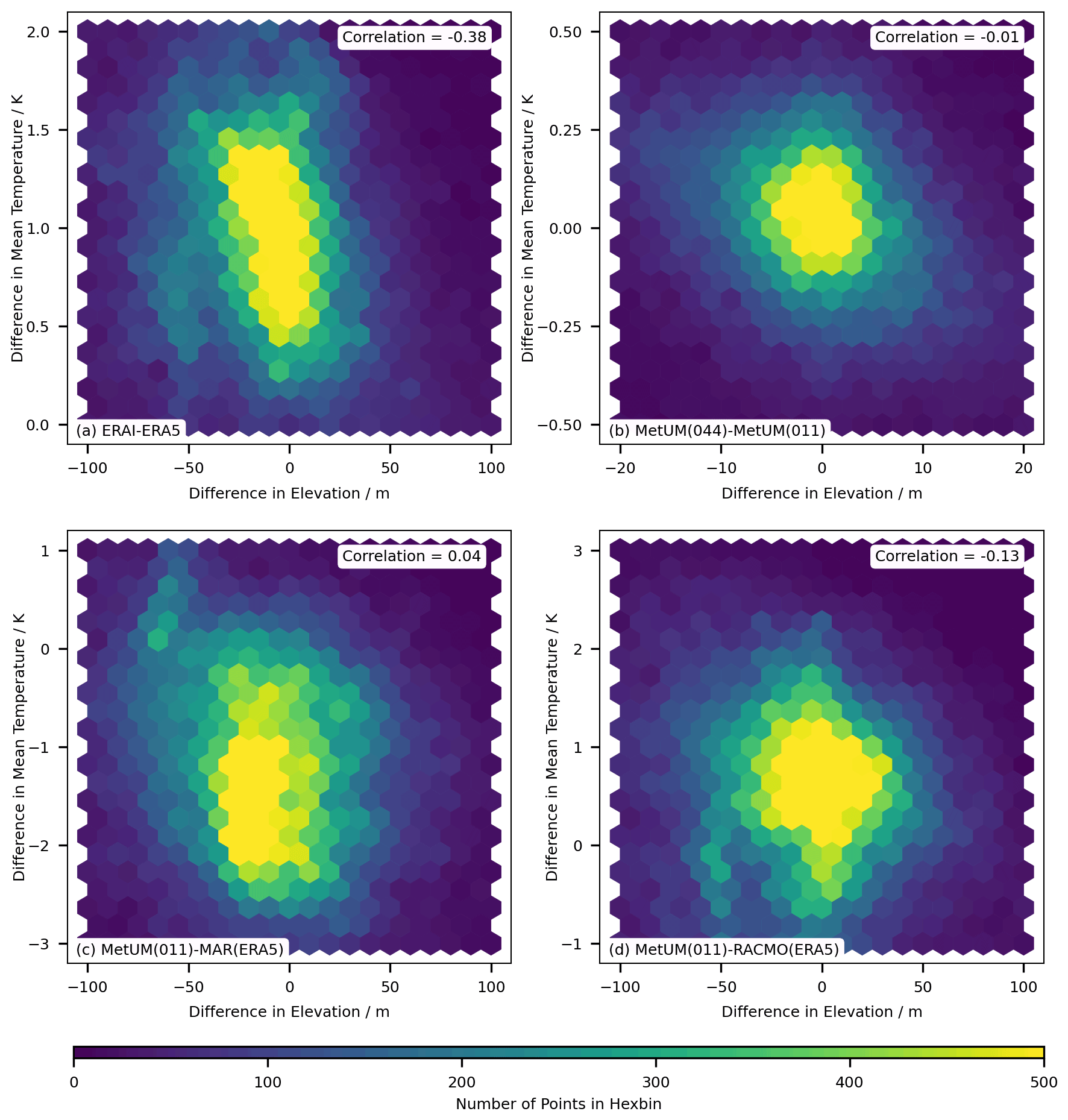
Figure C2 A density scatter plot showing the correlation between the difference in elevation for each model relative to the ensemble and the difference for near-surface temperature in the mean of the time series (a), the standard deviation of the seasonal component (b) and the standard deviation of the residual component (c). The linear Pearson correlation coefficient is given for each plot.