the Creative Commons Attribution 4.0 License.
the Creative Commons Attribution 4.0 License.
 | 14 Sep 2022
A new Level 4 multi-sensor ice surface temperature product for the Greenland Ice Sheet
Magnus Barfod Suhr
Ruth Mottram
Pia Nielsen-Englyst
Gorm Dybkjær
Darren Ghent
Jacob L. Høyer
The Greenland Ice Sheet (GIS) is subject to amplified impacts of climate change and its monitoring is essential for understanding and improving scenarios of future climate conditions. Surface temperature over the GIS is an important variable, regulating processes related to the exchange of energy and water between the surface and the atmosphere. Few local observation sites exist; thus spaceborne platforms carrying thermal infrared instruments offer an alternative for surface temperature observations and are the basis for deriving ice surface temperature (IST) products.
In this study several satellite IST products for the GIS were compared, and the first multi-sensor, gap-free (Level 4, L4) product was developed and validated for 2012. High-resolution Level 2 (L2) products from the European Space Agency (ESA) Land Surface Temperature Climate Change Initiative (LST_cci) project and the Arctic and Antarctic Ice Surface Temperatures from Thermal Infrared Satellite Sensors (AASTI) dataset were assessed using observations from the PROMICE (Programme for Monitoring of the Greenland Ice Sheet) stations and IceBridge flight campaigns. AASTI showed overall better performance compared to LST_cci data, which had superior spatial coverage and availability. Both datasets were utilised to construct a daily, gap-free L4 IST product using the optimal interpolation (OI) method. The resulting product performed satisfactorily when compared to surface temperature observations from PROMICE and IceBridge. Combining the advantages of satellite datasets, the L4 product allowed for the analysis of IST over the GIS during 2012, when a significant melt event occurred. Mean summer (June–August) IST was −5.5 ± 4.5 ∘C, with an annual mean of −22.1 ± 5.4 ∘C. Mean IST during the melt season (May–August) ranged from −15 to −1 ∘C, while almost the entire GIS experienced at least between 1 and 5 melt days when temperatures were −1 ∘C or higher.
Finally, this study assessed the potential for using the satellite L4 IST product to improve model simulations of the GIS surface mass balance (SMB). The L4 IST product was assimilated into an SMB model of snow and firn processes during 2012, when extreme melting occurred, to assess the impact of including a high-resolution IST product on the SMB model. Compared with independent observations from PROMICE and IceBridge, inclusion of the L4 IST dataset improved the SMB model simulated IST during the key onset of the melt season, where model biases are typically large and can impact the amount of simulated melt.
- Article
(7779 KB) - Full-text XML
- BibTeX
- EndNote


There has been an increase in the rate of Arctic ice loss over the last 2 decades, including the accelerated retreat of glaciers and ice sheets, a reduction in the extent and timing of seasonal snow, and a reduced sea ice extent and thickness as a result of climate change (IPCC, 2019). The Greenland Ice Sheet (GIS) has had a net negative mass balance for at least the last 25 years, resulting from the combination of increased dynamic thinning, i.e. loss due to accelerated flow and calving, and decreased surface mass balance (SMB) (Shepherd et al., 2020; Mottram et al., 2019; Mankoff et al., 2020). From September 2019 to August 2020 the GIS experienced ice loss higher than the average for the period from 1981 to 2010 (Moon et al., 2020).
SMB is the budget of accumulation (via snowfall) and ablation (via melt and runoff). Also important are processes of meltwater percolation into the snow and firn (snow that has survived at least one annual cycle) where meltwater can be retained as a liquid if there is sufficient pore space and may refreeze if the cold content is sufficient, potentially forming aerially extensive ice layers (Broeke et al., 2009; Ettema et al., 2010; Machguth et al., 2016; Reijmer et al., 2012). A decrease in SMB over the last 25 years is the largest contributor to the mass loss of the GIS, largely due to enhanced melting during the summer melt season (Shepherd et al., 2020). SMB is directly measured at only a few point locations in Greenland, and regional climate models (RCMs) are used to make integrated estimates over the whole ice sheet (Shepherd et al., 2020). However, as analysis by Fettweis et al. (2020) shows, there are large discrepancies between models in terms of both the components of SMB (mainly melt rates and precipitation) and the geographical pattern of SMB. Satellite observations over large areas are therefore essential for evaluating models and are also useful in process studies to identify sources of model error as well as being potentially useful in correcting model biases via assimilation in climate and weather models.
Land surface temperature (LST) can be observed by satellites and is classified as an Essential Climate Variable (ECV) according to the Global Observing System for Climate (GCOS) (GCOS, 2016). The temperature of the snow- and ice-covered land surfaces (ice surface temperature, IST), usually calculated from the surface energy balance from observations or RCMs, controls both melt rates and other snowpack processes that are important for characterising SMB. As firn provides an important buffer for meltwater, it must be included in SMB models to determine rates of ice sheet loss. However there is a wide variation in the performance of different firn models and the parameterisations used within them (Langen et al., 2017; Vernon et al., 2013). As an example, the retention and refreezing of liquid water are modulated by grain size and densification, which are in turn strongly influenced by surface temperatures over the GIS (Vandecrux et al., 2020). Improving modelled IST is therefore important for SMB estimates of the GIS.
Satellite observations in the thermal infrared (IR) have allowed monitoring of clear-sky ISTs over the last 4 decades. Infrared sensors operate in the atmospheric window where wavelengths range between 10 and 12 µm; thus measurements refer to the skin ice surface temperature, which may differ considerably from e.g. in situ stations which typically measure the 2 m air temperature. Furthermore, infrared measurements can only be obtained under clear-sky conditions and thus are representative of instances when temperature is typically lower compared to cloudy conditions (Nielsen-Englyst et al., 2019). Nielsen-Englyst et al. (2021) used clear-sky skin temperature observations from satellite infrared radiometers to derive daily mean clear-sky 2 m air temperatures (T2 m) in the Arctic, including the Greenland Ice Sheet.
The primary IR sensors used for estimating IST are the Advanced Very High Resolution Radiometer (AVHRR) available since August 1981 (Comiso and Hall, 2014; Dybkjær et al., 2012; Comiso, 2003), the Moderate Resolution Imaging Spectroradiometer (MODIS) available since 1999 (Hall et al., 2008, 2012, 2013), the (Advanced) Along Track Scanning Radiometer ((A)ATSR) available since 1991 (Dodd et al., 2019), and the Sea and Land Surface Temperature Radiometer (SLSTR) A/B as successors of the (A)ATSR series. Recently, the European Space Agency (ESA) funded the Land Surface Temperature Climate Change Initiative (LST_cci) project, part of the agency's Climate Change Initiative (CCI) programme, releasing initial versions of data products from several satellites that provide temperature information across land surfaces regionally and globally, with a temporal extent of 20 years (Perry et al., 2020).
Averaged clear-sky IST observations from AVHRR have previously been analysed and used to calculate climate trends in the Arctic (Comiso, 2003; Wang and Key, 2005). However, the clear-sky limitation of IR observations usually results in differences when compared to the averaged ISTs measured during all-sky conditions (Comiso, 2003; Koenig and Hall, 2010; Nielsen-Englyst et al., 2019), which may impact the accuracy of the observed trends (Liu et al., 2008). Furthermore, single-sensor IST observations have gaps due to missing data, typically resulting from overcast conditions; thus direct comparisons with in situ measurements are further complicated by data unavailability. Currently, no gap-free (Level 4, L4) IST product exists for the GIS.
This study presents the results from a user case study within the ESA LST_cci project regarding uptake of the first satellite multi-sensor, optimally interpolated L4 IST fields covering the GIS for the test year 2012, when an extreme melting event occurred. IST data from IR satellite sensors were used from the ESA LST_cci project as well as from the Arctic and Antarctic Ice Surface Temperatures from Thermal Infrared Satellite Sensors (AASTI) dataset (Dybkjaer et al., 2018; Dybkjær et al., 2014). The individual satellite IST products were inter-compared and validated against in situ measured radiometric surface temperatures from the PROMICE (Programme for Monitoring of the Greenland Ice Sheet) stations and IceBridge flight campaigns. The year 2012 was selected due to extensive surface melt over most of the ice sheet (Box et al., 2012; Nghiem et al., 2012; Hall et al., 2013), resulting in the lowest SMB on record, a challenging event for climate models, many of which underestimated the contribution of turbulent heat fluxes to melting, especially the sensible heat flux (Fausto et al., 2016). Finally, this study assessed the potential to integrate the L4 IST product into climate models by first evaluating against and then assimilating the daily L4 IST data into an SMB model forced by the RCM HIRHAM5 (Langen et al., 2015, 2017).
Table 1Input satellite data used for the derivation of the daily L4 IST product.
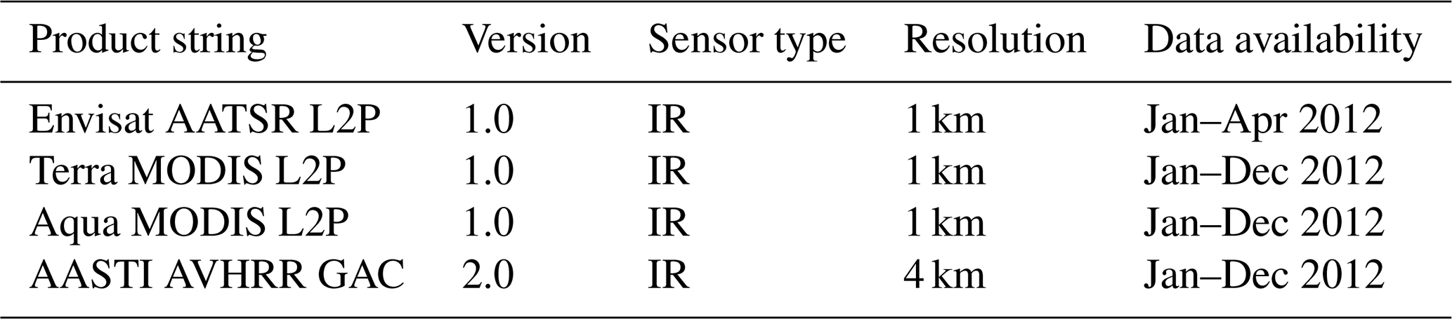
Table 2PROMICE observation sites including the surface type, co-ordinates and elevation.
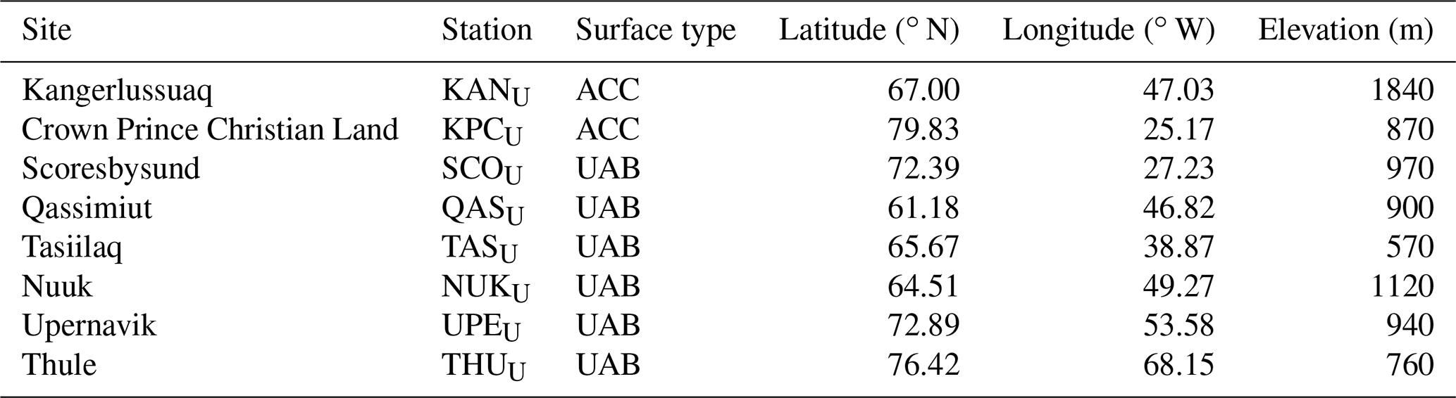
Surface type: upper or middle ablation zone (UAB), accumulation area (ACC).
2.1 Satellite data
As the GIS is located at high latitudes, it is not feasible to use aggregated day/night observations from ascending and descending orbits. L2 v1.0 data (without the subsequent enhancements to the algorithms, cloud masking and uncertainties) from the ESA LST_cci project were used, consisting of 1 km IST observations from AATSR on Envisat (only available until April 2012) and MODIS on the Aqua and Terra platforms (LST_cci, 2020). In addition, IST observations from the AASTI v2 L2 dataset, available multiple times per day with 4 km resolution, were included in the analysis (Dybkjaer et al., 2018; Dybkjær et al., 2014). This dataset is generated using Global Area Coverage (GAC) retrievals from AVHRR on board the NOAA and Metop platforms. The AASTI dataset extends north of 50∘ N and south of 50∘ S, providing surface temperatures for sea ice, land ice, open water and marginal ice zone areas from 1982 to 2015. The satellite products assessed in this study are listed in Table 1.
2.2 PROMICE
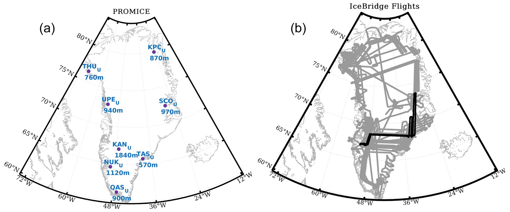
The Programme for Monitoring of the Greenland Ice Sheet (PROMICE) data are provided by the Geological Survey of Denmark and Greenland (Ahlstrøm et al., 2008; van As and Fausto, 2011; Fausto et al., 2021). Surface temperatures are derived from upwelling longwave radiation measured by Kipp & Zonen CNR1 or CNR4 radiometers, assuming an emissivity of 0.97 (Fausto et al., 2021). Only PROMICE data from the upper ablation and accumulation zones were used to ensure that data are only acquired over permanently snow- or ice-covered surfaces. Figure 1a shows the geographical distribution of the eight selected PROMICE stations and their elevation, also listed in Table 2.
2.3 IceBridge
The Operation IceBridge project (Kurtz et al., 2013) conducts flight campaigns over the Arctic sea ice and the GIS, carrying various instruments including a thermal infrared radiometer, KT19, which observes in a similar IR frequency interval as the AVHRR channel 4 (9.6–11.5 µm). Surface temperatures are retrieved by measuring brightness temperatures and assuming a constant surface emissivity of 0.97. In total, IST retrievals from 27 IceBridge flights (version 2) (Studinger, 2020) starting at the end of March and ending on 16 May 2012 were used. Due to the high-resolution footprint of the KT19 instrument – approximately 15 m at 450 m above ground level (Studinger, 2020) – which results in high variability in the observed radiometric surface temperature, IceBridge observations were averaged every kilometre to make them more comparable to the lower-resolution satellite data. The IceBridge observations were not screened for potential clouds; under the presence of clouds between the aircraft and the surface, the radiometer observes the usually colder cloud temperature instead of the surface.
3.1 Level 4 OI IST
L2 observations were aggregated on a fixed grid to Level 3 (L3) and combined using a statistical methodology similar to Høyer and Karagali (2016), resulting in L4 gap-free, merged and optimally interpolated (OI) daily fields with a 0.01∘ latitude and 0.02∘ longitude resolution. Prior to the optimal interpolation, an intermediate L3 super-collated (L3S) product was generated from the collation of all the L3 fields. The OI method is similar to the one from the high-latitude DMI SST (Danish Meteorological Institute sea surface temperature) processing scheme (Høyer and She, 2007; Høyer and Karagali, 2016), which operates with anomalies from a first-guess field. In the current approach, a persistence-based method is applied, which uses the previous analysis field as the first-guess field. The IST observations from within 48 h (hours) of the analysis time are aggregated and interpreted as anomalies with respect to the first-guess field. The OI method, given statistical input such as a first-guess error variance or co-variance functions and uncertainties in the individual observations, finds the solution with the lowest errors for each grid point (Høyer et al., 2014). The search radius for the OI method is set to 75 km, and the maximum number of satellite observations included in the optimal estimation is 16. A spatially and temporally varying dynamical bias correction has been applied to reference the MODIS products against the AASTI GAC data (Høyer et al., 2014). This occurs when constructing the L3S product prior to generating the L4 IST product. The temporal window for the dynamical correction is 7 d (days), and the bias fields are smoothed over 500 km. Due to the limited temporal availability and sampling pattern (see Sect. 4.1), AATSR data were not used for the generation of the L4 IST product.
The satellite products used in this study represent the clear-sky IST, as the IR satellite sensors cannot observe the surface through clouds. As a result, a clear-sky bias is usually observed when comparing averaged clear-sky surface temperatures against averaged all-sky temperatures (Koenig and Hall, 2010; Comiso, 2003). Nielsen-Englyst et al. (2019) used PROMICE observations to estimate the clear-sky bias introduced when averaging using different temporal windows. Using a 72 h averaging window, they found a clear-sky bias of −0.96 ∘C when PROMICE stations located in the middle or upper ablation zone and the accumulation zone were used. Here, this clear-sky bias of 0.96 ∘C has been added to the satellite products in order to provide an estimate of the corresponding all-sky daily IST fields, which can be compared to the all-sky ISTs observed by PROMICE and IceBridge.
3.2 HIRHAM5 regional climate model (RCM) and surface mass balance (SMB) model
The HIRHAM5 RCM simulates the climate of Greenland with a 5 km resolution (Mottram et al., 2017). The RCM contains a simplified SMB model and a five-layer snow and ice subsurface scheme. The surface energy and water budget from the RCM (i.e. the radiative and turbulent heat fluxes and precipitation), evaporation and sublimation outputs are then used to force an offline SMB model with more and deeper layers and a more sophisticated treatment of snowpack processes to calculate the ice sheet SMB. The full model set-up is described in Mottram et al. (2017); Langen et al. (2015, 2017).
The Lagrangian set-up with 32 unequally spaced layers down to 100 m of water equivalent depth in the snow and glacier subsurface scheme is used (Hansen et al., 2021). Assimilating an albedo product over bare glacier ice based on MODIS data can improve ice sheet surface melt estimates (Langen et al., 2017); however satellite-derived albedo data are not available as far back in the past and suffer from other biases. Thus, the focus in this study was exclusively on IST assimilation without albedo data assimilation; for the latter an internally calculated albedo scheme was used. The SMB model calculates the accumulation of snow and ablation based on the surface energy balance by calculating a theoretical skin temperature. Since the skin temperature of ice cannot go above 273.15 K, i.e. the melting point, this is converted to energy available for melting surface ice. The skin temperature also influences deeper snowpack temperatures via diffusion.
Meltwater is assumed to run off immediately if bare glacier ice is exposed, but if there is snow on glacier ice, percolation into the deep layers and the associated latent heat released by refreezing in deeper layers is accounted for until the heat capacity and porosity of the layers is filled and no more percolation is possible. The sum of precipitation minus evaporation, sublimation and runoff of meltwater gives the daily SMB over the ice sheet.
For the control simulation, surface energy balance outputs from the RCM were used to calculate the IST and melt potential as normal. This control simulation was initially evaluated against the L4 IST data (not shown). For the simulation with assimilation of the L4 IST, HIRHAM5 RCM forcing was initially used to calculate IST, and if this was below −2 ∘C at a grid point for a given time step, the L4 IST product was assimilated. Therefore, at any given time step, the GIS IST output by the SMB model is a combination of the modelled and observed L4 IST. The threshold was chosen to filter out biases at higher temperatures observed within the L4 IST product compared with PROMICE weather station data. The L4 IST product is available once daily, yet modelled IST is dependent on the full surface energy balance and thus, highly variable in space and time; assimilating the L4 IST product inevitably introduces some biases. Therefore, the aim of this assimilation experiment is to act as a proof of concept for the potential ingestion of satellite-derived data into the model. For this reason focus is on the month of May when IST and surface melt are highly variable; then the inclusion of satellite observations is likely to have the highest added value in identifying surfaces close to the melting point.
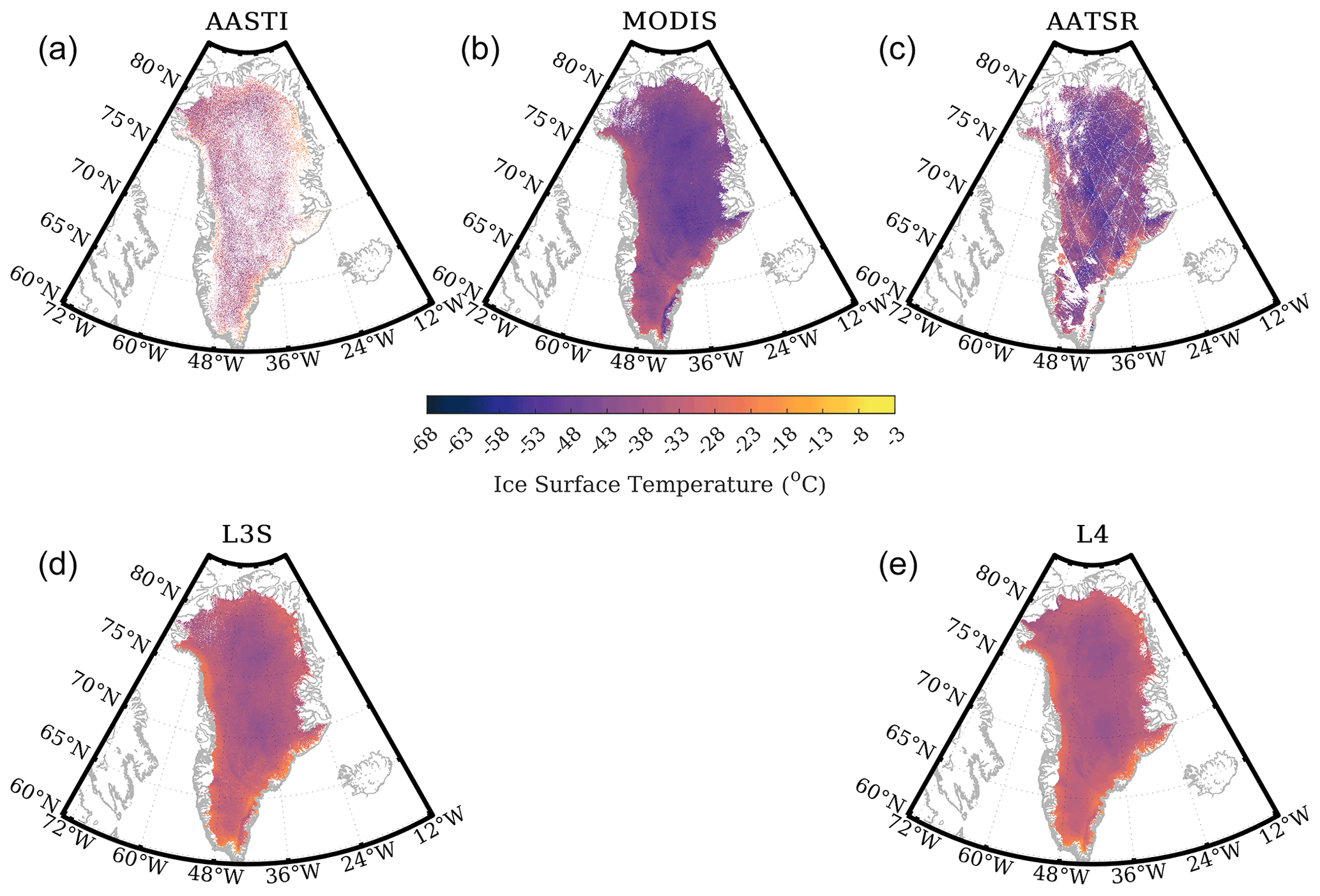
Figure 2Examples of aggregated IST observations from 9 January 2012 over the Greenland Ice Sheet. Top row: Level 3 AASTI (a), Level 3 MODIS on Aqua and Terra (b), Level 3 AATSR (c). Bottom row: Level 3S (d), Level 4 optimally interpolated IST (e).
4.1 Inter-comparison of IST products
Examples of the different L3 satellite products generated from the L2 datasets described in Table 1 are shown in Fig. 2. The L3 products are aggregated for 9 January 2012 – wintertime when cloud cover, impervious to IR radiation, is higher – into the L3S product (Fig. 2d), while after optimal interpolation, the L4 gap-free product (Fig. 2e) is produced for the same date. The coarser spatial resolution of AASTI (Fig. 2a) compared to MODIS (Fig. 2b) is visible, resulting in AASTI grid points with missing information, while MODIS daily aggregated L3 data offer superior coverage over the GIS. The sampling of AATSR (Fig. 2c) with its narrow swath and lower temporal resolution results in characteristic artefacts resembling the Envisat platform orbit. Such artefacts do not appear for either the MODIS or the AASTI products.
Figure 3 shows time series of mean daily ISTs and their standard deviation (shaded area) for 2012 from the aggregated AASTI L3, MODIS L3, AATSR L3, L3S and L4 IST. To estimate the mean daily IST for each dataset, a mask defining the Greenland Ice Sheet was applied, and all valid and available measurements were averaged to a daily value. Therefore, daily mean values shown in Fig. 3 are means over the entire area of consideration, and while the L4 IST product always has the same number of valid pixels used for the daily mean, the single-sensor products have a varying number of available measurements depending on data quality and cloud coverage. The L3S product is the combination of all single-sensor products, so its average is based on all available points from all single-sensor products.

Figure 3Mean daily IST (solid line) and its standard deviation (shaded area) over the Greenland Ice Sheet from the L3 AASTI, L3 MODIS, L3 AATSR (when available), and derived L3S and L4 IST products.
MODIS and AATSR (when available) show lower ISTs in particular during winter and late autumn compared to the other products, with minimum MODIS ISTs of about −50 ∘C and the AASTI and L3S and L4 IST products reaching their lowest ISTs of −35 to −40 ∘C. All products, including the L4 IST, represent well the annual cycle with warming starting in early March and peaking in July, followed by cooling and a winter minimum at the end of December.
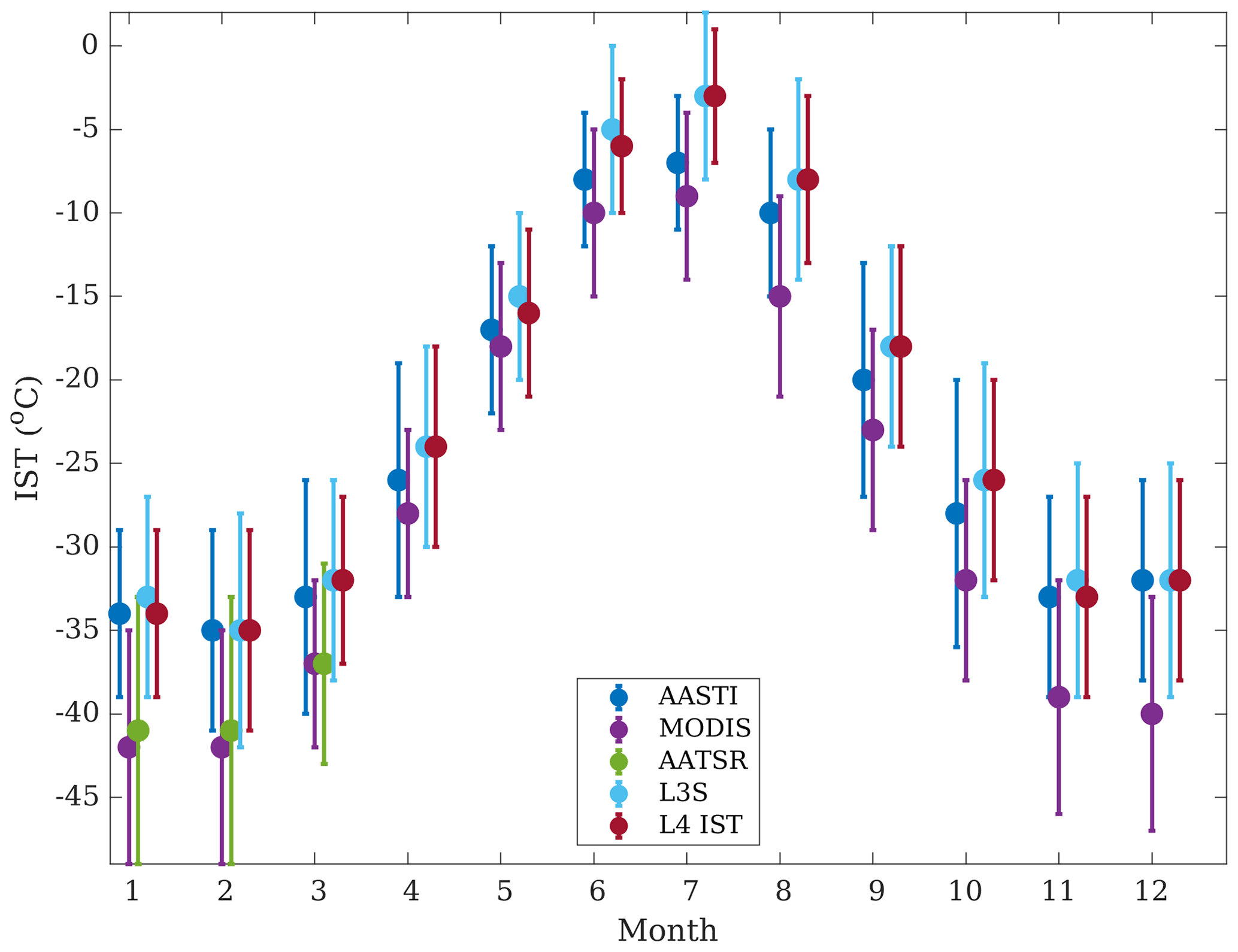
Figure 4Mean monthly IST (dots) and its standard deviation (bars) over the Greenland Ice Sheet from the L3 AASTI, L3 MODIS, L3 AATSR, and derived L3S and L4 IST products, when available.
The mean monthly IST and its standard deviation for all L3 products and the L4 IST are shown in Fig. 4. AATSR was only available until the beginning of April; thus no monthly value was calculated. From January to March, mean monthly ISTs from MODIS (magenta) and AATSR (green) were similar and significantly lower than AASTI (blue), the L3S (cyan) and the L4 IST product (red) accompanied by a higher standard deviation. These differences decreased from April to June, yet MODIS consistently showed lower values and higher variability compared to AASTI and the derived L3S and L4 products, which consistently agreed throughout the year. All products showed a peak mean monthly value in July, while June was warmer than August. From January to March, mean monthly temperatures were comparable to November–December means, and standard deviations were of the same order.
Such differences and variabilities are also reflected in the mean seasonal and annual estimates, shown in Table 3 for the different L3 products (excluding AATSR) and the L4 IST product. The AASTI, L3S and L4 IST products showed higher, as well as similar, seasonal and annual means compared to MODIS. Discrepancies between the estimates ranged from 0.5 ∘C in winter to ∼ 1 ∘C in summer, between the AASTI, L3S and L4 IST products. MODIS was 3–8 ∘C colder, with discrepancies being smallest in spring. Mean annual IST over the GIS ranged from −22.1 ± 5.4 ∘C for the L4 IST to −27.9 ± 5.9 ∘C from MODIS.
Table 3Mean annual and seasonal IST with standard deviation (∘C), from the different L3 and the L4 IST products for the Greenland Ice Sheet for 2012.
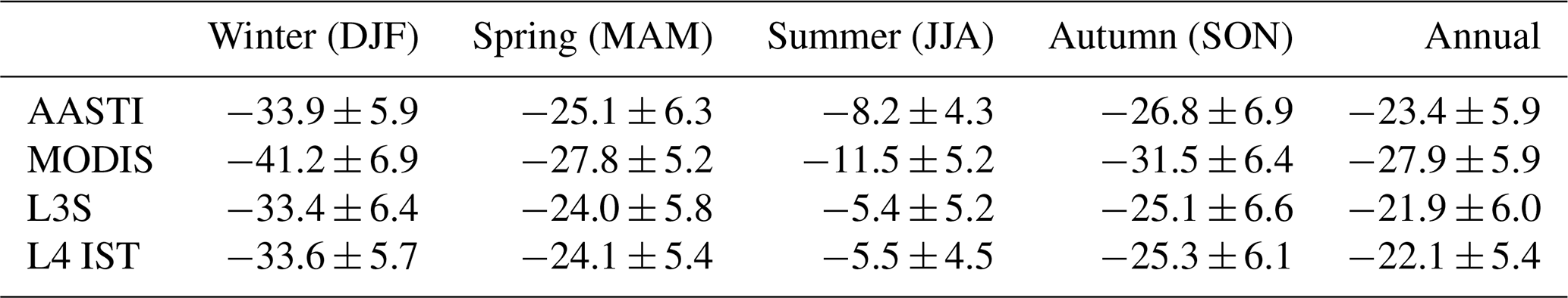
For all products, winter mean temperatures were determined by averaging January, February and December of 2012. AATSR was excluded, as data were only available until April. DJF: December–January–February, MAM: March–April–May, JJA: June–July–August, SON: September–October–November.
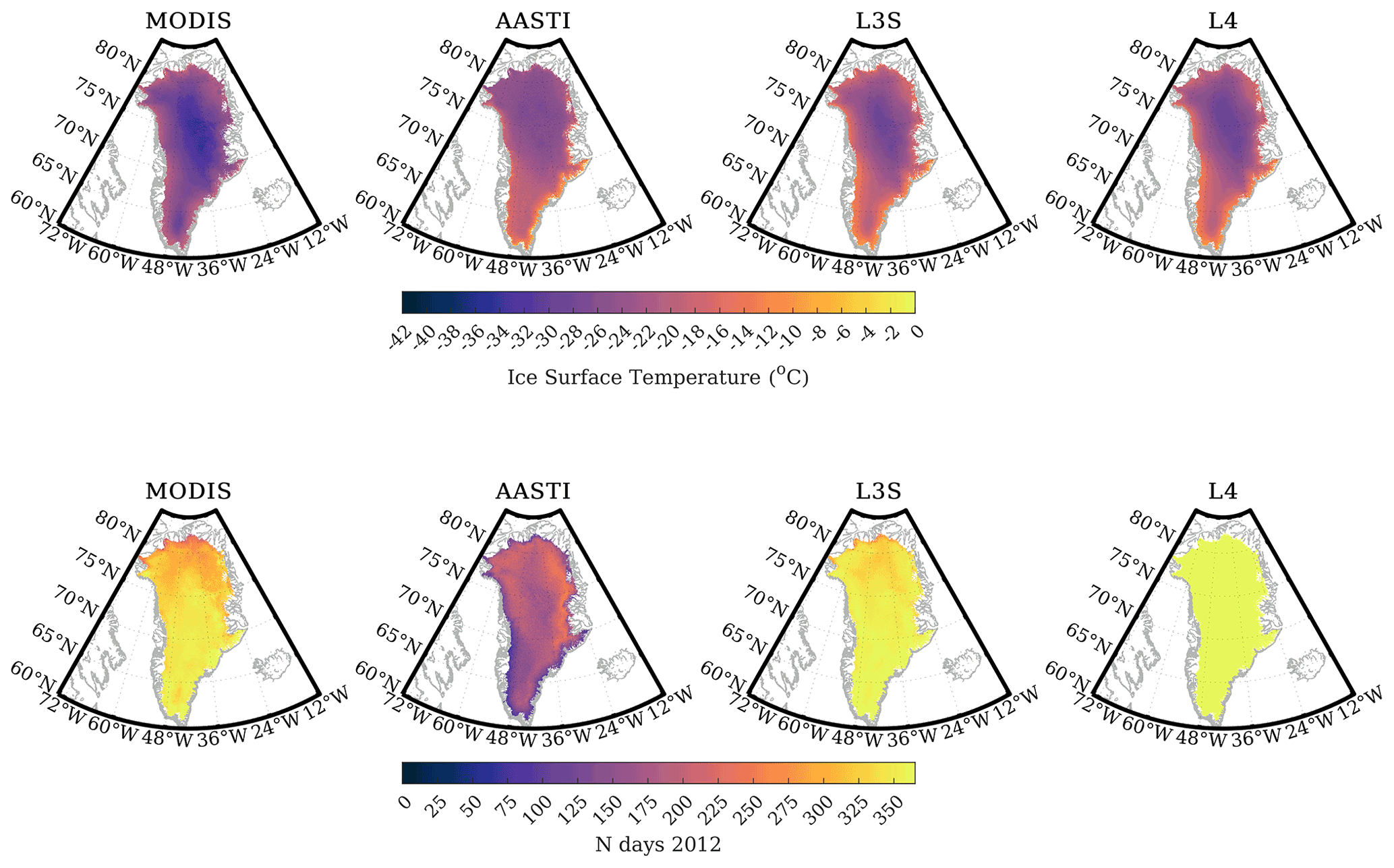
Figure 5Mean IST over the Greenland Ice Sheet in 2012 from the L3 MODIS, L3 AASTI, and derived L3S and L4 IST products (top) along with the number of days used to derive the mean values.
The spatial variability in mean annual IST over the Greenland Ice Sheet for 2012 from the AASTI, MODIS, L3S and L4 OI products is shown in Fig. 5 along with the number of days with observations used to derive the means. For the MODIS and AASTI datasets, the intermediate L3 gridded products were used for the estimates; i.e. the original 1 km and 4 km L2 observations were re-gridded to the 5 km final grid. MODIS mean IST was significantly lower over the entire Greenland Ice Sheet compared to the AASTI estimates, although significantly more observations were available for the former. Mean IST from the L3S and L4 OI products appear more similar to AASTI mean estimates.
The primary reason for the lower LST_cci v1.0 MODIS and AATSR IST values, used in the present study, is the type of cloud masking applied in the first version of the data. No post-filtering or implementation of the cloud-masking techniques (later developed within the LST_cci for both instruments) were applied in the v1.0 of the data presented here, but only the standard operational cloud mask was used; this frequently failed to properly flag clouds, which are typically colder, resulting in lower surface temperature values. For the case of AATSR, in addition to the cold bias, there also was the sampling issue (see Fig. 2) and the limited availability of data for the reference year 2012 (contact with Envisat was lost in April). Therefore, AATSR was not included in the final L3S and L4 IST product. With respect to the MODIS product, the pixel-to-pixel variability is smaller than for AASTI, mostly associated with the better coverage (see Fig. 2), and it was thus decided to use it for the generation of the L4 IST product.
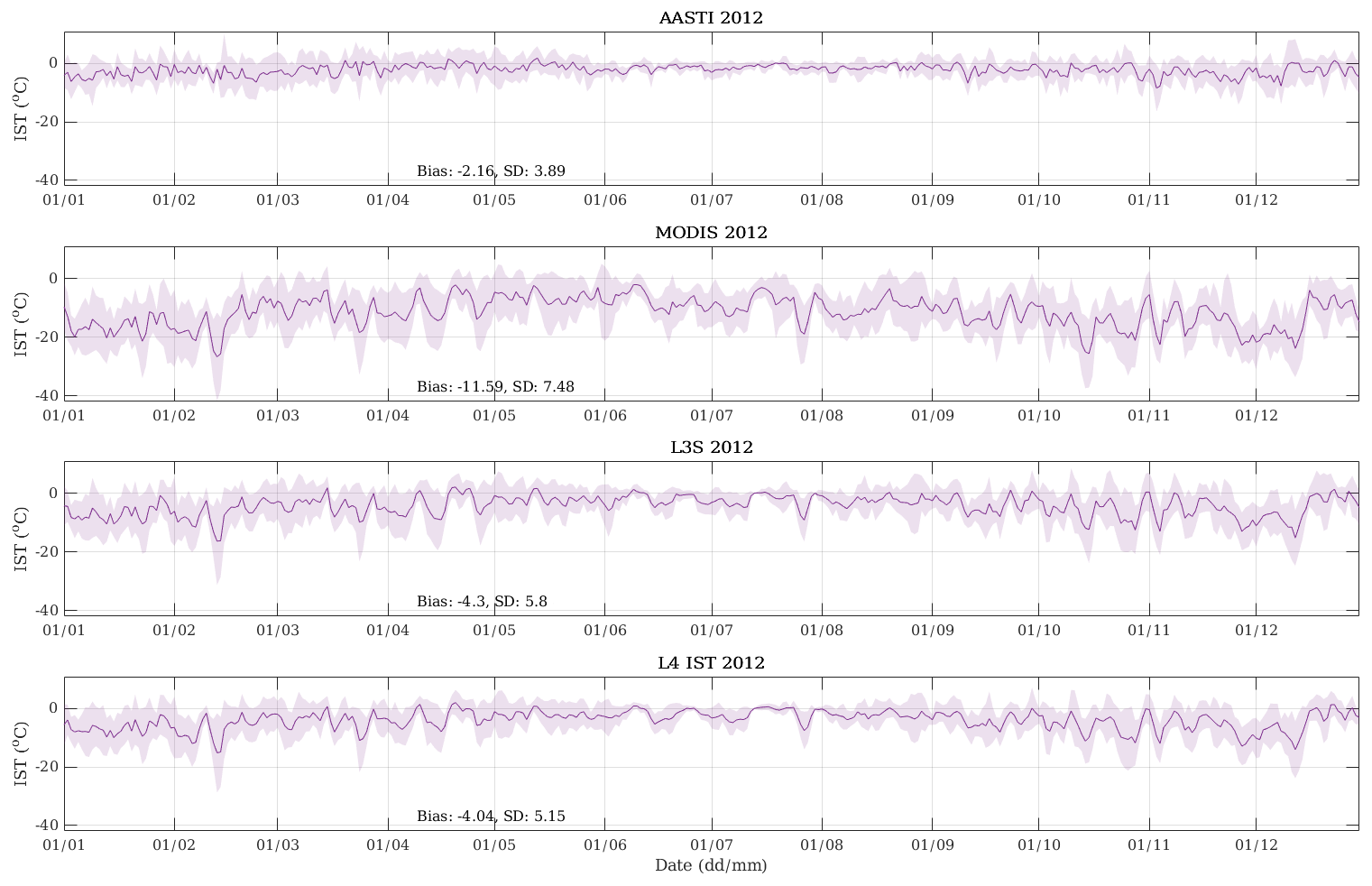
Figure 6Time series of mean daily bias estimates (line) and their standard deviation (shaded area) for the AASTI, MODIS, L3S and L4 IST products against aggregated in situ observations from the PROMICE stations.
4.2 Validation of IST products
Figure 6 shows aggregated daily mean biases and standard deviations for the AASTI, MODIS, L3S and L4 IST product against the PROMICE stations (see Fig. 1a and Table 2). Note that, for each day, all available PROMICE stations were used and that that number differs from day to day, as not all stations have availability for all days. The overall bias of AASTI data was −2.16 ± 3.89 ∘C, significantly smaller than −11.59 ± 7.48 ∘C reported for MODIS. The L3S product bias was −4.30 ± 5.80 ∘C, while the L4 IST product was also found cold with a mean bias of −4.04 ± 5.15 ∘C, i.e. 0.26 ∘C lower bias and 0.65 ∘C lower standard deviation compared to the L3S product. During summer, mean bias and standard deviation for AASTI was very stable and close to zero, which was not the case for MODIS. The L3S and L4 IST products also showed higher variability in the daily bias and standard deviation during summer, compared to AASTI, yet they appear more stable than MODIS, indicating the benefits of using the OI methodology to generate daily, gap-free IST fields. Furthermore, the lower bias and standard deviation of the L4 IST product against PROMICE stations, along with its better coverage, demonstrate its potential advantage over single-sensor products or daily aggregated fields.
Table 4Mean bias and standard deviation of errors for the AASTI, MODIS, L3S and L4 IST products against in situ observations for each of the PROMICE stations.
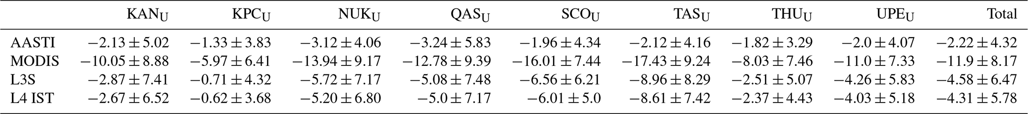
When examining the performance of the L3 and L4 products individually for each PROMICE station (Table 4), AASTI consistently had the lowest bias (from −3.24 to −1.34 ∘C) and standard deviation values (3.29–5.83 ∘C) for all stations, independent of altitude, type of ice sheet zone and geographical location. MODIS, beyond higher bias and standard deviation values, also showed higher variability, with biases ranging from −17.43 to −5.97 ∘C and standard deviations between 6.41 and 9.39 ∘C. Such behaviour provides additional evidence that the cold-bias issue stems from the early version of MODIS data used in this study and the cloud-masking approach implemented.
Other studies have shown similar cold biases in surface temperatures derived from MODIS (Wan et al., 2002; Hall et al., 2012, 2013). However, as shown in Sect. 4.1, the important contribution of the aggregated MODIS observations in achieving a proper coverage over the GIS justifies the dynamical bias correction of the MODIS product against the AASTI data described in Sect. 3.1 and its further use for the generation of the L4 IST product.
This higher variability in the MODIS product influenced the performance of both the L3S and the L4 IST product, where biases ranged from −8.61 to −0.62 ∘C and standard deviations from 3.68 to 7.42 ∘C. The overall performance using the PROMICE stations was −2.22 ± 4.32 ∘C for the AASTI, −11.9 ± 8.17 ∘C for the MODIS, −4.58 ± 6.47 ∘C for the L3S and −4.31 ± 5.78 ∘C for the L4 IST product. The stable performance of AASTI and the L4 IST indicated that no single station and its characteristics (location, altitude) influenced the validation statistics.

Figure 7Mean bias (dots) and standard deviation of errors (bars) for the AASTI, MODIS, L3 IST and L4 IST products against individual IceBridge flight observations from March to May 2012. The total bias and standard deviation values are reported.
Using the 1 km averaged surface temperature observations from 27 IceBridge flight campaigns, starting in 30 March and ending in 16 May, mean bias (dots) and standard deviation (vertical bars) were estimated and are shown in Fig. 7 for AASTI, MODIS, L3S and the L4 IST. For most flights, AASTI observations were in agreement with the IceBridge observations, with overall zero bias (−0.01 ± 4.03 ∘C) and a very stable behaviour, as no major outliers occurred; biases ranged from −2.10 to 2.10 ∘C. MODIS was cold compared to the flight measurements, manifesting as a negative bias (−5.19 ± 4.8 ∘C) and with a pronounced variability during the period evident from the oscillating bias (from −14.15 to 2.20 ∘C) and standard deviation values (from 2 to 7.2 ∘C).
The L3S and L4 IST products (bottom panels of Fig. 7) showed significantly lower bias and standard deviation compared to MODIS although with a similar, yet reduced, variability in the statistics depending on the campaign; biases ranged from −6.66 to 3.98 ∘C with standard deviations from 1.7 to 6.6 ∘C. Overall, the L3S product had a bias of −0.63 ± 4.27 ∘C, and the L4 IST had a bias of −0.61 ± 3.59 ∘C, i.e. the lowest standard deviation of all datasets considered, ∼ 0.44 and ∼ 0.6 ∘C lower than the AASTI and L3S product, respectively. As was the case for the PROMICE comparisons, the L4 IST product combined stability and robustness in its validation performance and along with its improved spatial coverage can be considered more relevant for applications, e.g. related to SMB modelling of the ice sheet.
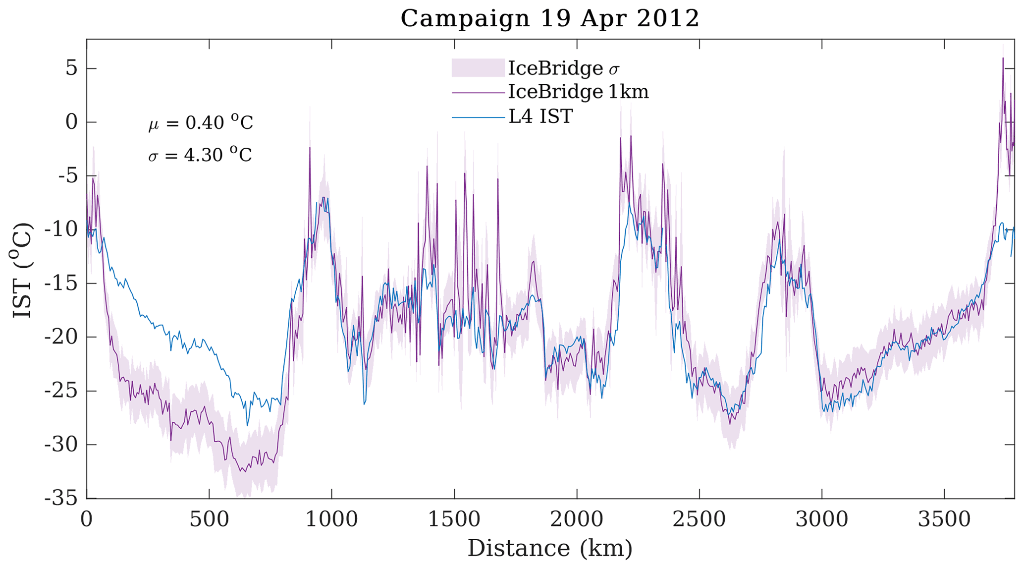
Figure 8IceBridge 1 km averaged IST on 19 April 2012 (magenta) and standard deviation (shaded area) along with the corresponding L4 IST values (blue).
An example of one IceBridge flight campaign is shown in Fig. 8 for 19 April 2012. Flight measurements, corresponding to the coloured flight path in Fig. 1b, averaged every 1 km as a function of distance covered during the flight (magenta) along with their standard deviation (shaded area), are shown along with values from the L4 IST product, extracted for the grid points corresponding to the flight path (blue line). The mean bias for that campaign was 0.40 ± 4.30 ∘C. This campaign, which started and ended on the western coast, covered various zones of the GIS, and the variability in the IST was intense as revealed by the 1 km averaged measurements. Beyond the warm bias during the first 800 km of the flight, the L4 IST captured the variability in the ISTs over the GIS remarkably well. As the IceBridge radiometer measures the radiometric surface temperature from an aircraft at an approximate height of 450 m a.g.l. without any cloud screening, the presence of clouds may explain the discrepancies for the first 800 km of the flight where the IceBridge data are significantly colder than the L4 IST.
In order to assess the impact of the high-resolution footprint of the IceBridge measurements on the validation statistics, i.e. 1 km averages over 5 km averages of the L3 and L4 IST products, the standard deviation of averaging raw measurements over different spatiotemporal windows minus the raw measurements were computed (not shown). This is an assessment of biases introduced from comparing flight data of very high resolution, i.e. resolving small-scale variability, against spaceborne sensors which, although referred to between 1 and 5 km grids, are known to resolve scales lower than their reference grid.
Using only IceBridge campaign data, averaging for different spatial windows, i.e. 1, 5 and 25 km, and subtracting raw measurements, the standard deviation values for each campaign were estimated (not shown). The largest component standard deviation was introduced when processing the raw data to 1 km averages, of the order of 2 ∘C. Depending on the campaign, an additional 0.1 to 0.6 ∘C of the standard deviation was attributed to the averaging from 1 to 5 km. When averaging from 1 to 25 km, differences in the standard deviation reached 0.9 ∘C while the mean difference in the standard deviation over all campaigns was averaging 0.22 ∘C from 1 to 5 km and 0.4 ∘C from 1 to 25 km. Thus, between 0.2 and 0.4 ∘C of the standard deviation in all comparisons against IceBridge campaigns (see Fig. 7) can be attributed to the different spatial scales represented in the IceBridge data compared to satellite observations.
The validation of the AASTI, MODIS, L3S and L4 IST datasets showed that for both PROMICE and IceBridge, AASTI had an overall better performance, with lower biases and standard deviations. MODIS v1.0 data from the LST_cci project, used in this study, had a significant cold bias, associated with the less advanced cloud mask algorithm applied to this early version; this influenced the performance of the derived L4 IST product. Nonetheless, the better spatial coverage and higher resolution of MODIS rendered it crucial for the generation of the L4 IST product, and thus its inclusion was justified. A new, improved version of the MODIS L2P dataset, to be released by the LST_cci, is expected to result in better performance of the L4 IST OI product.
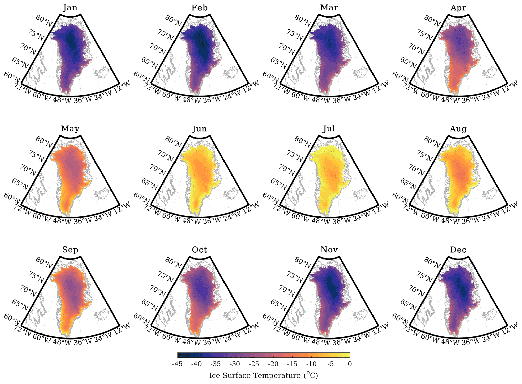
Figure 9Mean monthly ice surface temperature over the Greenland Ice Sheet for 2012, from the L4 IST product.
4.3 Analysis of the L4 IST
Monthly averages from the L4 IST product for 2012, shown in Fig. 9, indicate the extent of warming during the summer months where temperatures on the GIS ranged from −16 to 0 ∘C, especially during July and for most of the ice sheet. Similar ranges were reported in Hall et al. (2008) for the period 2000–2006 from MODIS LST products as well as in Hall et al. (2012), using daily MODIS IST between 2000 and 2010.
The number of aggregated observations from AASTI and MODIS used to generate the L4 IST product (not shown) revealed a seasonal pattern where most observations were available between May and August, while the fewest observations were available from November to February. The northern part of the GIS was consistently observed fewer times compared to the central part. This spatial and temporal variability in the availability of observations from MODIS and AASTI is related to the availability of observations in the infrared which is limited by cloud cover.
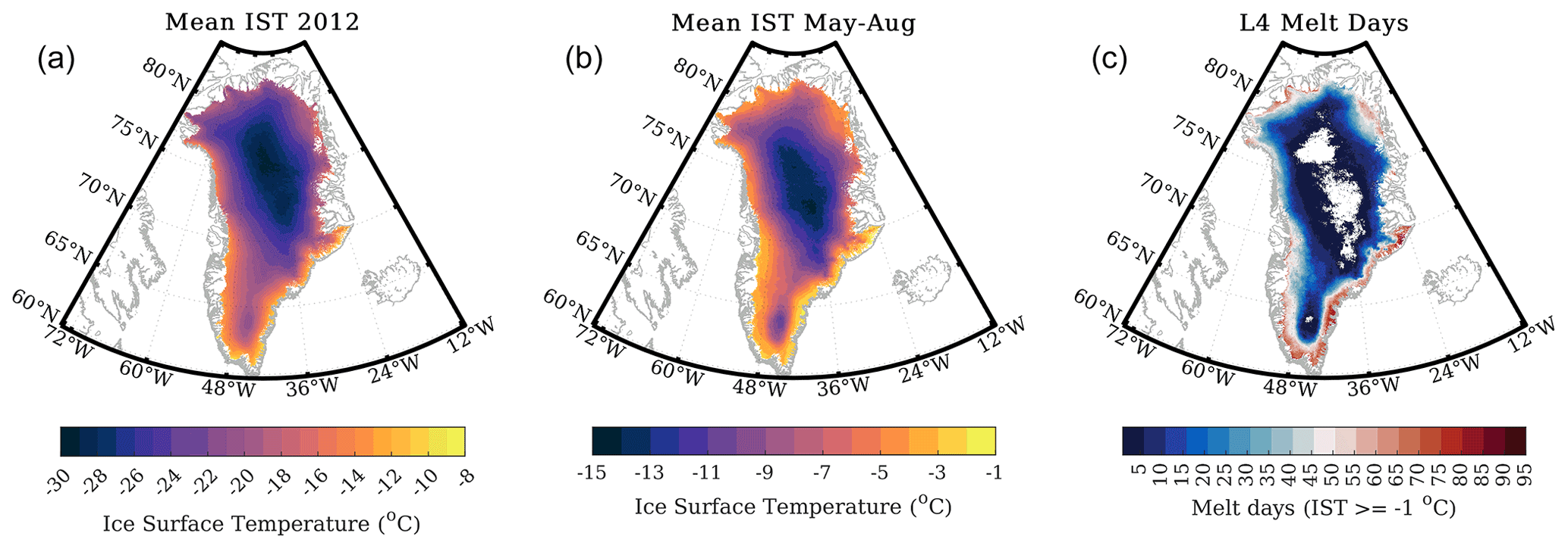
Figure 10Mean IST for 2012 (a) and for the melt season May–August 2012 (b) and number of melt days during the melt season (c, minimum 1 d, white areas on the GIS indicate 0 d) from the L4 IST product.
The annual mean IST over the GIS for 2012 is shown in Fig. 10a, using the L4 IST product. Values ranged from −30 ∘C for the central part of the ice sheet and increased up to −8 ∘C for the terminal zones, particularly for latitudes south of 70∘ N. Hall et al. (2008) reported similar values using MODIS data between 2000 and 2006. Furthermore, the mean IST during the melt period May–August 2012 (Fig. 10b) estimated from the L4 IST product showed values ranging from −15 and up to 0 ∘C, in agreement with Hall et al. (2008).
Melt days were defined as days for which the IST was −1 ∘C or higher, following Hall et al. (2013). They were estimated for the period 1 May to 31 August, at each grid point over the GIS. Figure 10c shows the number of melt days from the L4 IST product, where white areas experienced 0 melt days and coloured areas indicate at least 1 melt day. Melting was observed over large parts of the GIS for more than 1 d, while significant parts of the middle and lower zones experienced more than 30 d of melt conditions.
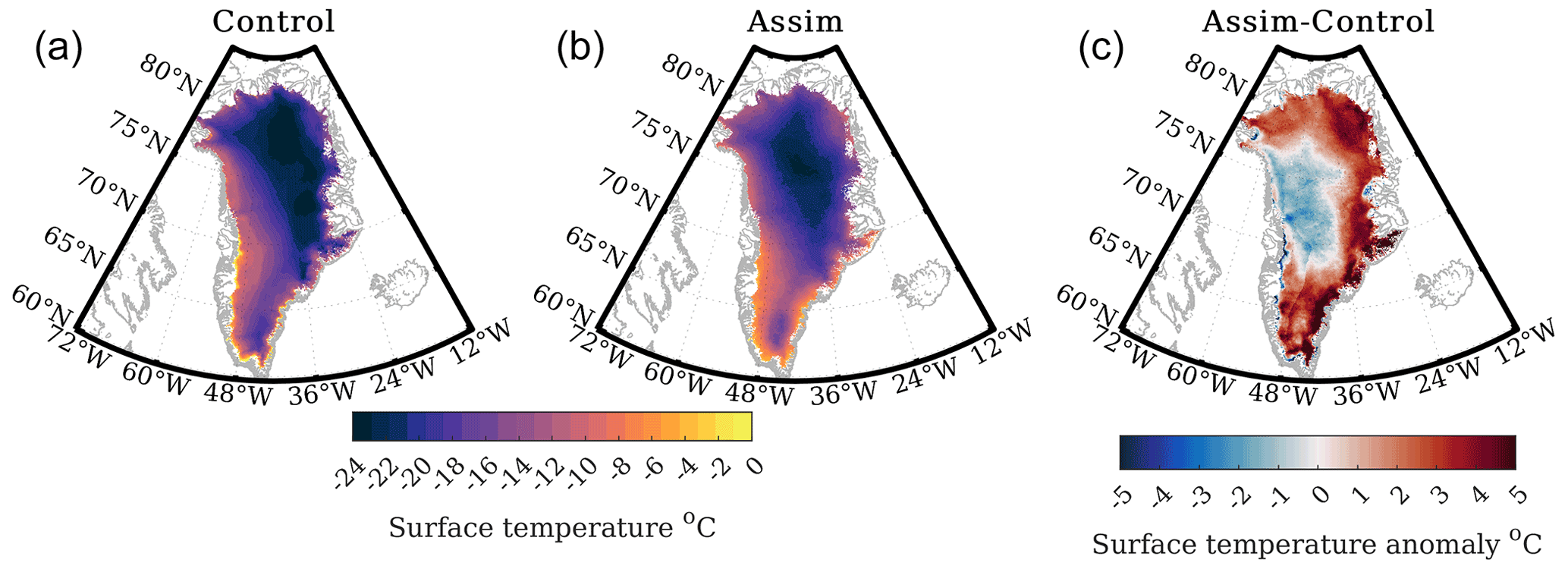
Figure 11Mean monthly surface temperature for May 2012 from the control (a) and updated simulation experiment (b) along with the anomaly (c).
Table 5Mean bias and standard deviation of errors for the control simulation and the one using the assimilation of the L4 IST against the individual PROMICE stations for May 2012.

4.4 IST assimilation experiment
Figure 11 shows mean monthly IST values for May, estimated from the control (Fig. 11a) and updated simulation (Fig. 11b), i.e. including assimilation of the L4 IST product; the estimated anomaly is shown in Fig. 11c. May was selected, as it is the month when the onset of melting commonly occurs across much of western and southern Greenland; this is a challenging period for SMB models to simulate, and the use of IST observations can potentially have a positive impact on the simulated IST and consequently the amount of simulated melt (not directly assessed in this study).
When examining the simulated surface temperature, the updated simulation using the assimilation of the L4 IST, was generally warmer over a large part of the GIS, especially the east and north-east regions. The difference between the two mean May surface temperature estimates, computed by subtracting mean May surface temperature estimates of the control simulation from the one using assimilation of the L4 IST (Fig. 11c), highlighted the areas for which the control simulation was consistently colder by 2 ∘C or more, even up to 5 ∘C, extending to the north, south and east parts of the GIS. To the contrary, the control simulation showed warmer temperatures on the west and central part of the GIS, yet differences in this case did not exceed 1 ∘C, and only for small areas were they up to 3 ∘C.
Comparing the simulated surface temperatures against the PROMICE stations for May 2012 (Table 5) showed that mean daily temperatures from both the control (top) and updated simulation (bottom), using assimilation of the L4 IST product, were colder compared to PROMICE station measurements. The bias was lower for the updated simulation (−1.14 ∘C) compared to the control simulation (−2.16 ∘C), yet the standard deviation was higher, 3.55 ∘C for the updated simulation compared to 2.9 ∘C for the control. Only at the TASU station did both simulations indicate warmer surface temperatures, but this needs to be assessed cautiously given the very few observations available in May 2012 at this station (not shown).
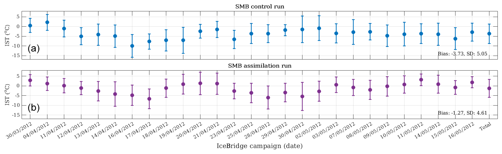
Figure 12Mean bias (dots) and standard deviation (bars) for the control simulation (a) and the one using the assimilation of the L4 IST (b) against the IceBridge flight campaigns.
Figure 12 shows a comparison of surface temperatures with the IceBridge flight campaign measurements to assess the control (Fig. 12a) and updated simulation (Fig. 12b), with assimilation of the L4 IST product; a marked improvement with the assimilation of L4 IST data was found, with a reduction in both the bias and the standard deviation compared to the control. The reduced standard deviation for the IceBridge data comparison, as compared to PROMICE observations, was consistent with what was reported in Sect. 4.2.
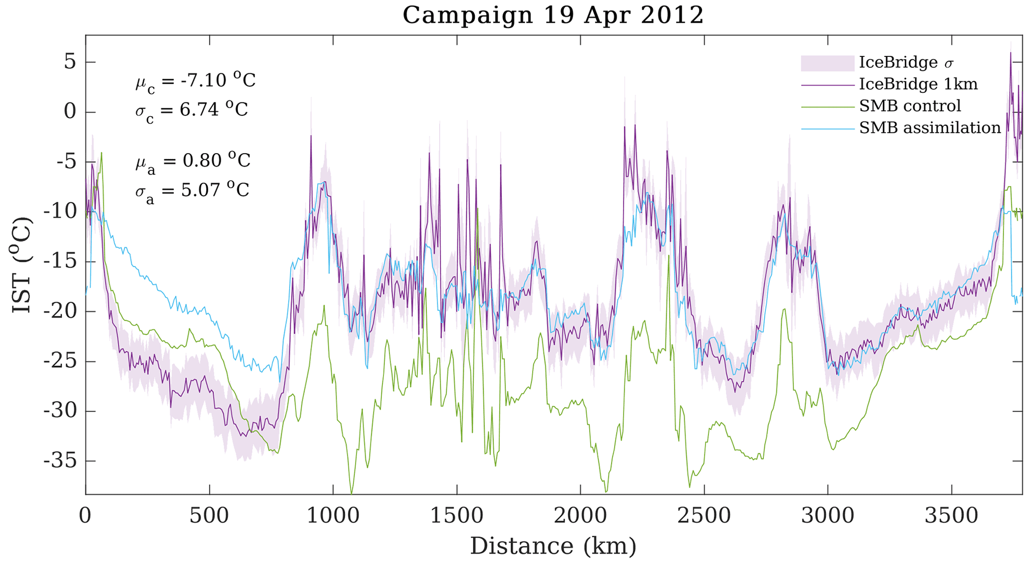
Figure 13IceBridge 1 km averaged IST on 19 April 2012 (magenta) and standard deviation (shaded area) along with the corresponding values from the control (green) and updated SMB simulations (cyan).
An example of surface temperature measurements from one IceBridge flight and the associated surface temperatures from the SMB simulations is shown in Fig. 13, similar to what was shown for the L4 IST in Fig. 8. Flight measurements, averaged every 1 km, as a function of distance covered during the flight (magenta) and their standard deviation (shaded area) are shown along with surface temperature values from the SMB model control (green) and updated simulation using assimilation of the L4 IST product (cyan), extracted for the grid points corresponding to the flight path. For this specific flight, the mean bias and standard deviation with respect to the IceBridge measurements was −7.10 ± 6.74 ∘C for the control simulation and −0.80 ± 5.07 ∘C for the updated one.
The L4 IST product was shown to improve the SMB model simulated surface temperatures when compared to PROMICE stations and IceBridge flight campaign measurements, for the test case of May 2012, selected as the typical onset of the melting season. Experiments for other months of 2012 (not shown) indicated a neutral impact of the L4 IST product, providing more confidence in the existing SMB internal parameterisations for the simulation of surface temperature, for the least challenging periods.
In this study, infrared observations from the reprocessed archive of the ESA LST_cci project and the AASTI dataset were utilised to demonstrate the capability for generating a Level 4 ice surface temperature product over the Greenland Ice Sheet, based on existing long-term, homogenised datasets from satellite sensors. The aim was to demonstrate the generation, quality and performance of the new L4 IST product compared to its single-sensor predecessors and in situ observations and finally the applicability of such a product for monitoring IST over Greenland and its potential utilisation in a surface mass balance model.
Validation of the upstream input datasets and the derived L4 IST indicated larger differences between the satellite products and PROMICE measurements during winter, which can likely be associated with the higher diurnal variability in IST during winter (Nielsen-Englyst et al., 2019) and the fact that cloud-masking algorithms can suffer from reduced skill to identify cloudy from clear-sky pixels over ice-covered surfaces during the polar winter season (Dybkjær et al., 2012).
The validation of satellite IST products against in situ observations suffers from the lack of available fiducial reference observations for the IST over the GIS. As discussed in Høyer et al. (2017), the use of pointwise in situ observations can introduce a sampling uncertainty ranging from 0.4 to 5 ∘C, depending on the type of in situ observations, when compared to satellite observations with a 1 km footprint. Such contributions are not related to the performance of the satellite products but arise from the spatial and temporal sampling uncertainty and the type of in situ observations.
For the types of in situ observations used for validation in this study, it is expected that the PROMICE broadband IST observations will have higher uncertainties compared to the IceBridge data. This is a consequence of the PROMICE broadband radiometer observations versus the narrowband IceBridge observations; the snow and ice surface emissivity effects, arising from surface properties or incidence angles, vary much more for the broadband observations compared to the narrowband radiometer. In addition, although the spectral response functions (SRFs) of the IceBridge KT19 instrument are very similar to the actual IR satellite SRFs, the instrument footprints are different. Therefore, the results from the inter-comparison should not be viewed as an estimate of the uncertainty in the satellite products.
Beyond the differences in the broadband PROMICE versus narrowband IceBridge measurements, another reason for the reduced standard deviation can be associated with the fact that the IceBridge flights also cover the interior of the ice sheet, where temperatures are lower and there is little melt. The PROMICE stations lie mostly within the ablation zone where there are large diurnal and seasonal changes in IST that are challenging for both model and satellite observations to characterise.
The choice of 75 km for the search radius of the optimal interpolation scheme was a compromise between selecting a large search radius that ensured enough data to be included in the OI estimate and a computationally feasible search grid box. The average number of observations found within the 75 km search radius is near the maximum number of available observations; thus the selected search radius is not severely limiting the number of observations available for the OI. The threshold of 75 km is being used for the operational production of the near-real-time Arctic Ocean L4 SST/IST (Høyer et al., 2021).
Analyses of the annual spatiotemporal variability in IST over the GIS revealed extended warming during the summer months of 2012, already reported as an extreme melt year (Box et al., 2012; Nghiem et al., 2012). Assessing mean annual IST values over the GIS for 2012, Hall et al. (2013) reported mean annual IST of −23.62 ± 6.24 ∘C from MODIS, which is closer to the L4 IST values, compared to what is derived from MODIS in this study. Hall et al. (2013) manually removed daily MODIS IST fields when the cloud mask erroneously identified the ice surface as cloud free, particularly occurring during the summer. Their 2012 summer season mean IST was −6.38 ± 3.98 ∘C, which is significantly higher than the −11.5 ± 5.2 ∘C found for MODIS in the present study and closer to the −5.5 ± 4.5 ∘C for the L4 IST product.
Both Hall et al. (2008), for the period 2000–2006, using MODIS LST products and Hall et al. (2012), using daily MODIS IST between 2000 and 2010, reported similar ranges of IST values over the GIS as found in this study. Furthermore, the 2012 annual mean IST over the GIS reported in this study (see Fig. 10a) is similar to what was derived in Hall et al. (2008) using MODIS observations for 2000–2006. For the melt period defined between May and August 2012, mean IST from the L4 IST product (Fig. 10g) was found to be in agreement with Hall et al. (2008) (see their Fig. 2), although for that study non-ice-covered land surface temperatures where also considered; thus above zero values were included.
Hall et al. (2013) reported more than 2 melt days for most of the GIS during the melt season of 2012, based on MODIS data, which also indicated the warmest summer in the MODIS record with a mean IST of −6.38 ± 3.98 ∘C, in good agreement with the mean summer IST from the L4 IST product reported in Table 3. In Nghiem et al. (2012), extended melt over the GIS was identified from a combination of spaceborne sensors, including MODIS in alignment with findings from this study (see Fig. 10). The extreme melt event of 2012 reported in this and past studies was associated with unusually high geopotential heights and atmospheric pressure anomalies over the ice sheet in Hanna et al. (2014).
As the year 2012 was significant in terms of melting over the GIS, the month of May specifically poses a challenge, as it signifies the onset of the melt season, i.e. a challenging period for SMB models to simulate correctly, as biases in winter accumulation can lead to significant discrepancies between observed and simulated melt onset. Hermann et al. (2018) showed that overestimates of winter snow close to the ice sheet margin delayed the onset of simulated melt compared to reality in southern Greenland, with the reverse bias being found higher up where snowfall rates were underestimated. The use of IST data to mitigate against this bias has the potential to improve annual melt and SMB estimates.
Both the control and updated simulation, using the L4 IST product, were forced by the HIRHAM5 RCM, which provides the required 6-hourly forcing fields and allows for calculation of surface temperature at a higher temporal resolution; this also captures the diurnal cycle, likely an important process to resolve in the ablation zone, especially in spring. The coarser temporal resolution of surface temperature assimilated into the model in the updated simulation using the L4 IST dataset, compared to the control run, can be considered a challenge for assimilating such products. This is a topic that needs careful consideration when aiming to generate optimally interpolated IST fields from spaceborne sensors for the purpose of providing input to models that are typically in need of temporally resolved parameters with a frequency higher than daily. Nonetheless, the high spatial coverage offered by the L4 IST product is an attractive and important attribute when aiming to capture and represent surface temperature variability over large areas of the GIS, as demonstrated in Sect. 4.3, that can not be resolved through in situ measuring stations and is typically underrepresented in large- (global) and medium-scale (mesoscale) model simulations.
The L4 OI IST dataset generated and presented here was the result of a user case from the ESA LST_cci project and was only generated for the selected year of 2012 to assess the impact and applicability of such a product over the Greenland Ice Sheet. Ideally such a product can be expanded to cover the entire period of available L2 input data, thus resulting in more climatologically relevant timescales of the order of 20 to 30 years. Such a task will become significantly more relevant during the second phase of ESA LST_cci, during which the current suite of products will be improved and temporally extended and new products will be included, e.g. the AVHRR series (NOAA 7–19 and Metop-A/B/C).
The ESA LST_cci v1.0 L2 MODIS Aqua/Terra data were used along with AASTI AVHRR GAC data to generate daily, gap-free, optimally interpolated L4 IST composites for the Greenland Ice Sheet (GIS) for the year 2012, chosen due to the extreme melt conditions. The upstream satellite data and the newly derived L4 product were validated using PROMICE and IceBridge observations. Furthermore, the L4 IST product was used to assess mean monthly, annual and seasonal IST over the GIS and provided the basis for estimating melt during 2012.
Comparisons against the PROMICE stations and airborne IST observations from the IceBridge flights suggest that the LST_cci MODIS data are cold biased by several degrees. This was attributed to the cloud-masking algorithm used for the generation of the v1.0 MODIS data within the LST_cci, as no post-filtering or techniques later developed by the LST_cci were implemented. The equivalent AASTI AVHRR data did not exhibit such a cold bias, and this demonstrates the importance of the multi-sensor inter-comparisons. After implementing a bias correction to the MODIS data, agreement between the derived L4 IST data and PROMICE stations and airborne IST measurements improved, but a residual cold bias was still evident in the L4 IST product. This suggests that the large number of MODIS observations included in the generation of the L4 IST, compared to AASTI, might challenge the bias adjustment scheme and that an improvement could be made regarding this in a future development. In general, we suggest that dedicated improvements on the IST retrievals and cloud-masking algorithms could reduce both the bias and the large regional errors presented in this study.
The larger biases and standard deviations identified for all satellite products against PROMICE stations compared to the ones for the IceBridge campaigns were associated with the higher uncertainties in the broadband radiometers used on the PROMICE stations. The IceBridge campaigns used a narrowband radiometer whose spectral response functions are very similar to the ones from thermal infrared satellite instruments. The locations of PROMICE stations in the ablation zone of the ice sheet can be the reason for larger diurnal variability in terms of surface energy budget that is not necessarily captured by a daily data product.
By combining upstream IST satellite products, the gap-free, daily L4 IST product exhibited a stable, high-quality performance when compared to the PROMICE stations and IceBridge flight measurements. Thus, advantages from AASTI (i.e. accuracy, stability and robustness) and MODIS (i.e. spatial resolution and coverage) were inherited in the L4 IST product. This allowed for a thorough analysis of IST spatial and temporal variability over the GIS during the challenging year of 2012. Findings were in agreement with other studies, which were nonetheless based on single-sensor satellite products. The L4 product is thus useful for understanding larger spatial and temporal variability over the GIS, not achievable using limited, local measurements or single-sensor satellite observations.
L4 IST daily fields were also ingested into an SMB model, forced by outputs from a regional climate model, to estimate ice melt and retention. The impact of using observed IST data in the model was assessed by comparing modelled and observed estimates of the surface temperature for 2012 when extreme melting occurred. A major challenge in this approach was the degradation in temporal resolution of surface temperature by forcing the assimilation of daily IST values from the gap-free L4 IST product. Nonetheless, for the melt onset period of May 2012 it was found that assimilating the daily L4 IST product produced more realistic surface temperatures when compared to PROMICE stations and IceBridge flight campaigns than the control simulation with an internal calculation of surface temperatures. This suggests that, while a continuous forcing of the SMB model with the daily L4 IST may not provide significant improvements at all locations and times of the year, at least when the temporal resolution of satellite IST products is daily, allowing for assimilation of the product during challenging periods of the year, e.g. onset and during the melt season, can improve SMB estimates through better surface temperature estimates.
Furthermore, a significant value for the L4 IST dataset was identified as a means to evaluate climate and SMB models and to conduct process studies. Even with coarser temporal resolution, IST data assimilation was found to improve surface temperatures over the large interior of the ice sheet, and this is in itself an important result. Sensitivity studies, e.g. changing the time step of assimilation and accounting for the time of IST data acquisition, are likely to further improve the use of IST data in weather and climate models.
PROMICE data are available from https://doi.org/10.22008/promice/data/aws (Fausto et al., 2022, 2021). Operation IceBridge data are available from https://doi.org/10.5067/UHE07J35I3NB (Studinger, 2020). ESA LST_cci data are available from the JASMIN facility http://gws-access.jasmin.ac.uk/public/esacci_lst/ (LST_cci, 2020). AASTI AVHRR GAC data are available upon request. The generated L4 IST dataset is to be distributed through the dedicated ESA LST_cci repositories, pending upload. SMB model simulations are available on request.
JLH and RM devised the initial concept for this study. DG provided the ESA LST_cci data and final comments. JLH designed and produced the L4 IST. RM designed and executed the simulation experiments. IK performed the inter-comparison of L4 and L3 and analysis of the L4 IST. MBS and PNE performed the validation of L3 and L4. MBS prepared inputs for and analysed the SMB simulations. IK led the authoring of the manuscript with contributions from MBS, RM, PNE, GD and JLH. All authors have read and agreed to the published version of the paper.
At least one of the (co-)authors is a member of the editorial board of The Cryosphere. The peer-review process was guided by an independent editor, and the authors also have no other competing interests to declare.
Publisher's note: Copernicus Publications remains neutral with regard to jurisdictional claims in published maps and institutional affiliations.
Funding was provided by the ESA CCI+ Phase 1 New Essential Climate Variables (New ECVS) LST project (ESA contract no. 400123553/18/I-NB) and the Danish National Centre for Climate Research (NCKF) at the Danish Meteorological Institute.
This research has been supported by the European Space Agency (ESA contract no. 400123553/18/I-NB) and the National Centre for Climate Research (Nationalt Center for Klimaforskning, Forskningsreserven; Danish Finance Law 2020–2021).
This paper was edited by Tobias Bolch and reviewed by two anonymous referees.
Ahlstrøm, A. P., Gravesen, P., Andersen, S. B., van As, D., Citterio, M., Fausto, R. S., Nielsen, S., Jepsen, H. F., Kristensen, S. S., Christensen, E. L., Stenseng, L., Forsberg, R., Hanson, S., and Petersen, D.: A new programme for monitoring the mass loss of the Greenland ice sheet, Geol. Surv. Den. Greenl., 15, 61–64, https://doi.org/10.34194/geusb.v15.5045, 2008. a
Box, J. E., Cappelen, J., Chen, C., Decker, D., Fettweis, X., Mote, T., Tedesco, M., van de Wal, R. S. W., and Wahr, J.: Greenland Ice Sheet in Arctic Report Card 2012, Arctic Report Card, NOAA, http://www.arctic.noaa.gov/reportcard (last access: November 2021), 2012. a, b
Broeke, M. V. D., Bamber, J., Ettema, J., Rignot, E., Schrama, E., Berg, W. J. D. V., Meijgaard, E. V., Velicogna, I., and Wouters, B.: Partitioning recent Greenland mass loss, Science, 326, 984–986, https://doi.org/10.1126/science.1178176, 2009. a
Comiso, J. C.: Warming trends in the Arctic from clear sky satellite observations, J. Climate, 16, 3498–3510, https://doi.org/10.1175/1520-0442(2003)016<3498:WTITAF>2.0.CO;2, 2003. a, b, c, d
Comiso, J. C. and Hall, D. K.: Climate trends in the Arctic as observed from space, WIREs Clim. Change, 5, 389–409, https://doi.org/10.1002/wcc.277, 2014. a
Dodd, E. M., Veal, K. L., Ghent, D. J., Broeke, M. R. V. D., and Remedios, J. J.: Toward a Combined Surface Temperature Data Set for the Arctic From the Along-Track Scanning Radiometers, J. Geophys. Res.-Atmos., 124, 6718–6736, https://doi.org/10.1029/2019JD030262, 2019. a
Dybkjær, G., Tonboe, R., and Høyer, J. L.: Arctic surface temperatures from Metop AVHRR compared to in situ ocean and land data, Ocean Sci., 8, 959–970, https://doi.org/10.5194/os-8-959-2012, 2012. a, b
Dybkjær, G., Høyer, J. L, Tonboe, R., and Olsen, S.: Report on the documentation and description of the new Arctic Ocean dataset combining SST and IST, NACLIM Deliverable D32.28, http://naclim.eu (last access: September 2022), 2014. a, b
Dybkjaer, G., Eastwood, S., Tonboe, R. T., Høyer, J. L., Borg, A. L., Englyst, P. N., Lavelle, J., and Jensen, M. B.: Arctic and Antarctic ice Surface Temperatures from AVHRR thermal Infrared satellite sensors 1982–2015, AGUFM, https://ui.adsabs.harvard.edu/abs/2018AGUFMGC24C..01D/abstract (last access: November 2021), 2018. a, b
Ettema, J., van den Broeke, M. R., van Meijgaard, E., and van de Berg, W. J.: Climate of the Greenland ice sheet using a high-resolution climate model – Part 2: Near-surface climate and energy balance, The Cryosphere, 4, 529–544, https://doi.org/10.5194/tc-4-529-2010, 2010. a
Fausto, R., van As, D., Box, J., Colgan, W., and Langen, P.: Quantifying the surface energy fluxes in South Greenland during the 2012 high melt episodes using in-situ observations, Front. Earth Sci., 4, 84, https://doi.org/10.3389/feart.2016.00082, 2016. a
Fausto, R. S., van As, D., Mankoff, K. D., Vandecrux, B., Citterio, M., Ahlstrøm, A. P., Andersen, S. B., Colgan, W., Karlsson, N. B., Kjeldsen, K. K., Korsgaard, N. J., Larsen, S. H., Nielsen, S., Pedersen, A. Ø., Shields, C. L., Solgaard, A. M., and Box, J. E.: Programme for Monitoring of the Greenland Ice Sheet (PROMICE) automatic weather station data, Earth Syst. Sci. Data, 13, 3819–3845, https://doi.org/10.5194/essd-13-3819-2021, 2021. a, b, c
Fausto, R. S., Van As, D., Mankoff, K. D.: AWS one boom tripod v03, V2, GEUS Dataverse [data set], https://doi.org/10.22008/FK2/8SS7EW, 2022. a
Fettweis, X., Hofer, S., Krebs-Kanzow, U., Amory, C., Aoki, T., Berends, C. J., Born, A., Box, J. E., Delhasse, A., Fujita, K., Gierz, P., Goelzer, H., Hanna, E., Hashimoto, A., Huybrechts, P., Kapsch, M.-L., King, M. D., Kittel, C., Lang, C., Langen, P. L., Lenaerts, J. T. M., Liston, G. E., Lohmann, G., Mernild, S. H., Mikolajewicz, U., Modali, K., Mottram, R. H., Niwano, M., Noël, B., Ryan, J. C., Smith, A., Streffing, J., Tedesco, M., van de Berg, W. J., van den Broeke, M., van de Wal, R. S. W., van Kampenhout, L., Wilton, D., Wouters, B., Ziemen, F., and Zolles, T.: GrSMBMIP: intercomparison of the modelled 1980–2012 surface mass balance over the Greenland Ice Sheet, The Cryosphere, 14, 3935–3958, https://doi.org/10.5194/tc-14-3935-2020, 2020. a
GCOS: The Global Observing System For Climate Implementation Needs, World Meteorological Organization, 200, 1–325, https://unfccc.int/files/science/workstreams/systematic_observation/application/pdf/gcos_ip_10oct2016.pdf (last access: November 2021), 2016. a
Hall, D. K., Williams, R. S., Luthcke, S. B., and Digirolamo, N. E.: Greenland ice sheet surface temperature, melt and mass loss: 2000-06, J. Glaciol., 54, 81–93, https://doi.org/10.3189/002214308784409170, 2008. a, b, c, d, e, f, g
Hall, D. K., Comiso, J. C., Digirolamo, N. E., Shuman, C. A., Key, J. R., and Koenig, L. S.: A satellite-derived climate-quality data record of the clear-sky surface temperature of the Greenland ice sheet, J. Climate, 25, 4785–4798, https://doi.org/10.1175/JCLI-D-11-00365.1, 2012. a, b, c, d
Hall, D. K., Comiso, J. C., DiGirolamo, N. E., Shuman, C. A., Box, J. E., and Koenig, L. S.: Variability in the surface temperature and melt extent of the Greenland ice sheet from MODIS, Geophys. Res. Lett., 40, 2114–2120, 2013. a, b, c, d, e, f, g
Hanna, E., Fettweis, X., Mernild, S. H., Cappelen, J., Ribergaard, M. H., Shuman, C. A., Steffen, K., Wood, L., and Mote, T. L.: Atmospheric and oceanic climate forcing of the exceptional Greenland ice sheet surface melt in summer 2012, Int. J. Climatol., 34, 1022–1037, https://doi.org/10.1002/joc.3743, 2014. a
Hansen, N., Langen, P. L., Boberg, F., Forsberg, R., Simonsen, S. B., Thejll, P., Vandecrux, B., and Mottram, R.: Downscaled surface mass balance in Antarctica: impacts of subsurface processes and large-scale atmospheric circulation, The Cryosphere, 15, 4315–4333, https://doi.org/10.5194/tc-15-4315-2021, 2021. a
Hermann, M., Box, J. E., Fausto, R. S., Colgan, W. T., Langen, P. L., Mottram, R., Wuite, J., Noël, B., Van Den Broeke, M. R., and van As, D.: Application of PROMICE Q-Transect in Situ Accumulation and Ablation Measurements (2000–2017) to Constrain Mass Balance at the Southern Tip of the Greenland Ice Sheet, J. Geophys. Res.-Earth, 123, 1235–1256, https://doi.org/10.1029/2017JF004408, 2018. a
Høyer, J. L. and Karagali, I.: Sea surface temperature climate data record for the North Sea and Baltic Sea., J. Climate, 29, 2529–2541, https://doi.org/10.1175/JCLI-D-15-0663.1, 2016. a, b
Høyer, J. L. and She, J.: Optimal interpolation of sea surface temperature for the North Sea and Baltic Sea, J. Marine Syst., 65, 176–189, https://doi.org/10.1016/j.jmarsys.2005.03.008, 2007. a
Høyer, J. L., Borgne, P. L., and Eastwood, S.: A bias correction method for Arctic satellite sea surface temperature observations, Remote Sens. Environ., 146, 201–213, https://doi.org/10.1016/j.rse.2013.04.020, 2014. a, b
Høyer, J. L., Alerskans, E., Nielsen-Englyst, P., Thejll, P., Dybkjær, G., and Tonboe, R.: Detailed investigation of the uncertainty budget for Non-recoverable IST observations and their SI traceability, http://www.frm4sts.org/wp-content/uploads/sites/3/2018/08/OP-70-FRM4STS_option3_report_v1-signed.pdf (last access: November 2021), 2017. a
Høyer, J. L., Karagali, I., and Nielsen-Englyst, P.: Product User Manual (PUM) for Arctic Sea and Ice Surface Temperature SEAICE_ARC_SEAICE_L4_NRT_OBSERVATIONS_011_008, version 1.6, Copernicus Marine Service [data set], https://doi.org/10.48670/moi-00130, 2021. a
IPCC: IPCC Special Report on the Ocean and Cryosphere in a Changing Climate, Intergovernmental Panel on Climate Change, https://www.ipcc.ch/srocc/ (last access: November 2021), 2019. a
Koenig, L. S. and Hall, D. K.: Comparison of satellite, thermochron and air temperatures at Summit, Greenland, during the winter of 2008/09, J. Glaciol., 56, 735–741, https://doi.org/10.3189/002214310793146269, 2010. a, b
Kurtz, N., Richter-Menge, J., Farrell, S., Studinger, M., Paden, J., Sonntag, J., and Yungel, J.: IceBridge airborne survey data support Arctic sea ice predictions, Eos T. Am. Geophys. Un., 94, 41–41, https://doi.org/10.1002/2013EO040001?sid=semanticscholar, 2013. a
Langen, P. L., Mottram, R., Christensen, J. H., Boberg, F., Rodehacke, C. B., Stendel, M., van As, D., Ahlstrøm, A. P., Mortensen, J., Rysgaard, S., Petersen, D., Svendsen, K. H., Aðalgeirsdóttir, G., and Cappelen, J.: Quantifying energy and mass fluxes controlling Godthåbsfjord freshwater input in a 5-km simulation (1991–2012), J. Climate, 28, 3694–3713, https://doi.org/10.1175/JCLI-D-14-00271.1, 2015. a, b
Langen, P. L., Fausto, R., Vandecrux, B., Mottram, R., and Box, J.: Liquid Water Flow and Retention on the Greenland Ice Sheet in the Regional Climate Model HIRHAM5: Local and Large-Scale Impacts, Front. Earth Sci., 4, 3694–3713, https://doi.org/10.3389/feart.2016.00110, 2017. a, b, c, d
Liu, Y., Key, J. R., and Wang, X.: The influence of changes in cloud cover on recent surface temperature trends in the Arctic, J. Climate, 21, 705–715, 2008. a
LST_cci: Product Validation and Intercomparison Report (PVIR), WP4B.2 – DEL4.1, ESA, https://admin.climate.esa.int/media/documents/LST-CCI-D4.1-PVIR_-_i1r0_-_Product_Validation_and_Intercomparison_Report.pdf (last access: November 2021), 2020. a, b
Machguth, H., Macferrin, M., van As, D., Box, J. E., Charalampidis, C., Colgan, W., Fausto, R. S., Meijer, H. A., Mosley-Thompson, E., and van de Wal, R. S.: Greenland meltwater storage in firn limited by near-surface ice formation, Nat. Clim. Change, 6, 390–393, https://doi.org/10.1038/nclimate2899, 2016. a
Mankoff, K. D., Solgaard, A., Colgan, W., Ahlstrøm, A. P., Khan, S. A., and Fausto, R. S.: Greenland Ice Sheet solid ice discharge from 1986 through March 2020, Earth Syst. Sci. Data, 12, 1367–1383, https://doi.org/10.5194/essd-12-1367-2020, 2020. a
Moon, T. A., Tedesco, M., Box, J. E., Cappelen, J., Fausto, R. S., Fettweis, X., Korsgaard, N. J., Loomis, B., Mankoff, K. D., Mote, T., Reijmer, C. H., Smeets, C. J. P. P., van As, D., and van de Wal, R. S.: Greenland Ice Sheet in Arctic Report Card 2020, Arctic Report Card, NOAA, https://doi.org/10.25923/ms78-g612, 2020. a
Mottram, R., Boberg, F., Langen, P., Yang, S., Rodehacke, C., Christensen, J., and Madsen, M.: Surface Mass balance of the Greenland ice Sheet in the Regional Climate Model HIRHAM5: Present State and Future Prospects, Low Temperature Science, 75, 105–115, https://doi.org/10.14943/lowtemsci.75.105, 2017. a, b
Mottram, R., Simonsen, S. B., Høyer Svendsen, S., Barletta, V. R., Sandberg Sørensen, L., Nagler, T., Wuite, J., Groh, A., Horwath, M., Rosier, J., Solgaard, A., Hvidberg, C. S., and Forsberg, R.: An Integrated View of Greenland Ice Sheet Mass Changes Based on Models and Satellite Observations, Remote Sens.-Basel, 11, 1407, https://doi.org/10.3390/rs11121407, 2019. a
Nghiem, S. V., Hall, D. K., Mote, T. L., Tedesco, M., Albert, M. R., Keegan, K., Shuman, C. A., DiGirolamo, N. E., and Neumann, G.: The extreme melt across the Greenland ice sheet in 2012, Geophys. Res. Lett., 39, L20502, https://doi.org/10.1029/2012GL053611, 2012. a, b, c
Nielsen-Englyst, P., Høyer, J. L., Madsen, K. S., Tonboe, R., Dybkjær, G., and Alerskans, E.: In situ observed relationships between snow and ice surface skin temperatures and 2 m air temperatures in the Arctic, The Cryosphere, 13, 1005–1024, https://doi.org/10.5194/tc-13-1005-2019, 2019. a, b, c, d
Nielsen-Englyst, P., Høyer, J. L., Madsen, K. S., Tonboe, R. T., Dybkjær, G., and Skarpalezos, S.: Deriving Arctic 2 m air temperatures over snow and ice from satellite surface temperature measurements, The Cryosphere, 15, 3035–3057, https://doi.org/10.5194/tc-15-3035-2021, 2021. a
Perry, M., Ghent, D. J., Jiménez, C., Dodd, E. M., Ermida, S. L., Trigo, I. F., and Veal, K. L.: Multisensor thermal infrared and microwave land surface temperature algorithm intercomparison, Remote Sens.-Basel, 12, 4164, https://doi.org/10.3390/rs12244164, 2020. a
Reijmer, C. H., van den Broeke, M. R., Fettweis, X., Ettema, J., and Stap, L. B.: Refreezing on the Greenland ice sheet: a comparison of parameterizations, The Cryosphere, 6, 743–762, https://doi.org/10.5194/tc-6-743-2012, 2012. a
Shepherd, A., Ivins, E., Rignot, E., Smith, B., Van Den Broeke, M., Velicogna, I., Whitehouse, P., Briggs, K., Joughin, I., Krinner, G., Nowicki, S., Payne, T., Scambos, T., Schlegel, N., A, G., Agosta, C., Ahlstrøm, A., Babonis, G., Barletta, V. R., Bjørk, A. A., Blazquez, A., Bonin, J., Colgan, W., Csatho, B., Cullather, R., Engdahl, M. E., Felikson, D., Fettweis, X., Forsberg, R., Hogg, A. E., Gallee, H., Gardner, A., Gilbert, L., Gourmelen, N., Groh, A., Gunter, B., Hanna, E., Harig, C., Helm, V., Horvath, A., Horwath, M., Khan, S., Kjeldsen, K. K., Konrad, H., Langen, P. L., Lecavalier, B., Loomis, B., Luthcke, S., McMillan, M., Melini, D., Mernild, S., Mohajerani, Y., Moore, P., Mottram, R., Mouginot, J., Moyano, G., Muir, A., Nagler, T., Nield, G., Nilsson, J., Noël, B., Otosaka, I., Pattle, M. E., Peltier, W. R., Pie, N., Rietbroek, R., Rott, H., SandbergSørensen, L., Sasgen, I., Save, H., Scheuchl, B., Schrama, E., Schröder, L., Seo, K.-W., Simonsen, S. B., Slater, T., Spada, G., Sutterley, T., Talpe, M., Tarasov, L., van de Berg, W. J., van der Wal, W., van Wessem, M., Vishwakarma, B. D., Wiese, D., Wilton, D., Wagner, T., Wouters, B., Wuite, J., and The IMBIE Team: Mass balance of the Greenland Ice Sheet from 1992 to 2018, Nature, 579, 233–239, https://doi.org/10.1038/s41586-019-1855-2, number: 7798 Publisher: Nature Publishing Group, 2020. a, b, c
Studinger, M.: IceBridge KT19 IR Surface Temperature, NASA National Snow and Ice Data Center Distributed Active Archive Center, Boulder, Colorado USA [data set], https://doi.org/10.5067/UHE07J35I3NB, version 2, 2020. a, b, c
van As, D. and Fausto, R. S.: Programme for Monitoring of the Greenland Ice Sheet (PROMICE): First temperature and ablation records, Geol. Surv. Den. Greenl., 23, 73–76, https://doi.org/10.34194/geusb.v23.4876, 2011. a
Vandecrux, B., Mottram, R., Langen, P. L., Fausto, R. S., Olesen, M., Stevens, C. M., Verjans, V., Leeson, A., Ligtenberg, S., Kuipers Munneke, P., Marchenko, S., van Pelt, W., Meyer, C. R., Simonsen, S. B., Heilig, A., Samimi, S., Marshall, S., Machguth, H., MacFerrin, M., Niwano, M., Miller, O., Voss, C. I., and Box, J. E.: The firn meltwater Retention Model Intercomparison Project (RetMIP): evaluation of nine firn models at four weather station sites on the Greenland ice sheet, The Cryosphere, 14, 3785–3810, https://doi.org/10.5194/tc-14-3785-2020, 2020. a
Vernon, C. L., Bamber, J. L., Box, J. E., van den Broeke, M. R., Fettweis, X., Hanna, E., and Huybrechts, P.: Surface mass balance model intercomparison for the Greenland ice sheet, The Cryosphere, 7, 599–614, https://doi.org/10.5194/tc-7-599-2013, 2013. a
Wan, Z., Zhang, Y., Zhang, Q., and liang Li, Z.: Validation of the land-surface temperature products retrieved from terra moderate resolution imaging spectroradiometer data, Remote Sens. Environ., 83, 163–180, https://doi.org/10.1016/S0034-4257(02)00093-7, 2002. a
Wang, X. and Key, J. R.: Arctic surface, cloud, and radiation properties based on the AVHRR polar pathfinder dataset. Part II: Recent trends, J. Climate, 18, 2575–2593, https://doi.org/10.1175/JCLI3439.1, 2005. a