Evaluation of six geothermal heat flux maps for the Antarctic Lambert–Amery glacial system

Basal thermal conditions play an important role in ice sheet dynamics, and they are sensitive to geothermal heat flux (GHF). Here we estimate the basal thermal conditions, including basal temperature, basal melt rate, and friction heat underneath the Lambert–Amery Glacier system in eastern Antarctica, using a combination of a forward model and an inversion from a 3D ice flow model. We assess the sensitivity and uncertainty of basal thermal conditions using six different GHF maps. We evaluate the modelled results using all observed subglacial lakes. The different GHF maps lead to large differences in simulated spatial patterns of temperate basal conditions. The two recent GHF fields inverted from aerial geomagnetic observations have the highest GHF, produce the largest warm-based area, and match the observed distribution of subglacial lakes better than the other GHFs. The modelled basal melt rate reaches 10 to hundreds of millimetres per year locally in the Lambert, Lepekhin, and Kronshtadtskiy glaciers feeding the Amery Ice Shelf and ranges from 0–5 mm yr⁻¹ on the temperate base of the vast inland region.

1 Introduction

The Lambert–Amery system in eastern Antarctica is believed to be relatively stable against climate change and has changed little over several decades of observations (King et al., 2007). However, there is also evidence of extensive subglacial canyons and lakes (Fretwell et al., 2013; Jamieson et al., 2016; Cui et al., 2020a). Subglacial canyons and lakes are conduits for subglacial water, transporting subglacial meltwater to the coast through complex hydrologic routing, which may change on relatively fast timescales (Malczyk et al., 2020). Jamieson et al. (2016) report a large subglacial drainage network in Princess Elizabeth Land (PEL), which would transport water from central PEL to the coast passing the Lambert–Amery region. Subglacial water can affect the ice flow (Stearns et al., 2008; Diez et al., 2018), influence the dynamical stability and basal mass balance (Gudlaugsson et al., 2017), and may enhance basal melt of ice shelves (Le Brocq et al., 2013).

Ice temperature is an important factor in the rheology of ice (Budd et al., 2013) and ice flow. Whether the basal ice is at the melting point influences the movement of the ice to a great extent. Ice at the melting point can lead to water flowing along hydraulic gradients and accumulating in local depressions (Fricker et al., 2016). The meltwater lubricates the ice/bed interface or saturates any sediment till layer, allowing higher ice velocities via basal sliding. For instance, the rapid retreat of Thwaites and Pope glaciers in the Amundsen Sea sector of western Antarctica is being facilitated by high heat flow in the underlying lithosphere (Dziadek et al., 2021). This bed–ice linkage forms the basis for making inferences on basal conditions via surface observations (Pattyn, 2010) or relict landforms (e.g. Näslund et al., 2005).

The ice temperature is controlled by deformational heat generated from strain within the ice, advection of heat due to lateral ice motion and the descent rate of ice from the surface, conduction of heat through the ice, and frictional heating from basal sliding. Ice temperature is hard to evaluate because of the scarcity of in situ measurements, which are typically obtained from boreholes that are very rarely drilled through the Antarctic ice sheet. Geothermal heat flux (GHF) is an important boundary condition for ice temperature simulation and is generally the largest source of uncertainty. Hence, geophysical survey methods are used to indirectly map GHF. To date, GHF datasets have been estimated from seismic models (Shapiro and Ritzwoller, 2004; An et al., 2015; Shen et al., 2020) and derived from airborne magnetic surveys (Li et al., 2021; Martos et al., 2017) and satellite geomagnetic data (Maule et al., 2005; Purucker, 2012).

Extensive ice-penetrating radar data have been collected recently over Princess Elizabeth Land (PEL; Fig. 1d), including the eastern part of the Lambert–Amery system (Cui et al., 2020a). This fills in large data gaps from older surveys and provides the basis for our study. The radar surveys reveal ∼ 1100 km long canyons (Fig. 1c) that are incised hundreds of metres deep into the subglacial bed that extend from the Gamburtsev Subglacial Mountains (GSM) to the coast of the Western Ice Shelf (WIS). Li et al. (2021) collected airborne magnetic data that can be combined with radar ice thicknesses and estimated depths at which the bedrock reaches its Curie temperature to invert for the geothermal flux. The resulting higher-resolution dataset (Li et al., 2021) implies a larger heat flux than previous estimates in this region. Furthermore, recently discovered subglacial lakes, including potentially the second-largest subglacial lake in Antarctica, add evidence for more widespread basal melting in the region than was thought based on the much sparser earlier survey data (Cui et al., 2020b). The complex subglacial topography, relatively high geothermal heat flux, and subglacial lakes imply a complex distribution of basal thermal conditions and subglacial water networks. These heterogenous basal conditions will have shaped much of the ice flow and mass balance of the Lambert–Amery system. This motivates us to investigate how the basal thermal conditions inferred from the new high-resolution topography dataset (Cui et al., 2020a) can be reconciled with surface ice velocities and existing geothermal heat flow maps.

Ice sheet models can be used to simulate the dynamics and thermodynamics of the ice sheet. Glaciologists have combined ice sheet models with measurements of vertical temperature profiles or thawed basal states to constrain the GHF of the ice sheets (e.g. Pattyn, 2010; Rezvanbehbahani et al., 2019). In the Lambert–Amery glacial system, Pittard et al. (2016) suggest that ice flow is most sensitive to the spatial variation in the underlying GHF near the ice divides and along the edges of the ice streams.

In this study, we simulate ice basal temperatures and basal melt rates in the Lambert–Amery system using the new high-resolution digital elevation model, along with six different published GHF maps as forcing for an offline coupling between a basal energy and water flow model and a 3D full Stokes ice flow model. We evaluate the quality of the resulting basal temperature field incorporating the Stokes model estimates of ice advection, strain, and frictional heating under the different GHF maps using all available observed subglacial lakes and surface velocities. Hence, we make inferences on which GHF maps yield the best match with observations in the region.

2 Regional domain and datasets

Our modelled domain is part of the Lambert–Amery system. It consists of two drainage basins, namely the Lambert Glacier basin and the American Highland basin, along with about half of the Amery Ice Shelf (Fig. 1). The 2D domain boundary outlines are defined by the inland ice catchment basin boundary, the central streamline, and the ice front of Amery Ice Shelf. The central streamline was chosen by selecting a point at the confluence of Lambert Glacier and Lepekhin Glacier and then advecting that point downstream to the ice front using the observed velocity field. The margins of the inland subbasin and the central streamline of the Amery Ice Shelf were chosen as boundaries because the mass flux across them is assumed to be zero by definition.

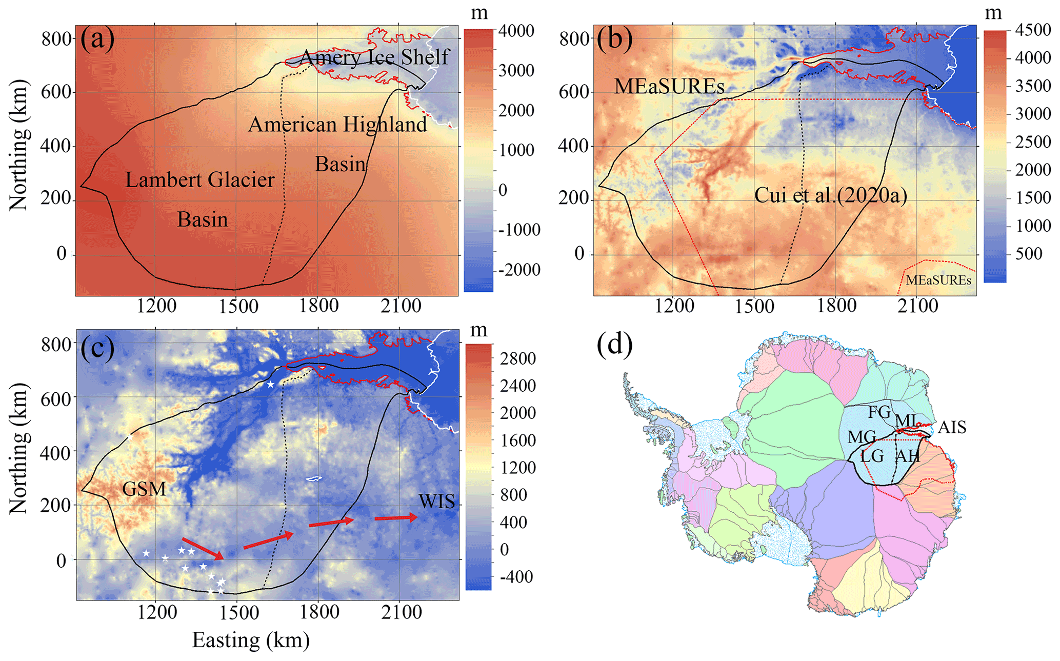
Figure 1 The domain topography and location with domain boundary overlain. (a) Surface elevation. (b) Ice thickness. (c) Bed elevation. (d) The location of our domain in Antarctica. The solid black curve is the outline of the study domain, including the central streamline of Amery Ice Shelf and the boundary of inland subbasins based on drainage basin boundaries defined from satellite ice sheet surface elevation and velocities (Mouginot et al., 2017; Rignot et al., 2019). The solid red and white curves in panels (a)–(c) are the grounding line and margin of Antarctic, respectively (Morlighem et al., 2020). The dotted black curve is the dividing line between Lambert Glacier basin and the American Highland basin. The dotted red curves in panels (b) and (d) are the boundary of ice thickness data from Cui et al. (2020a), inside which we incorporate data from Cui et al. (2020a) and outside from MEaSUREs BedMachine Antarctica, version 2. The white stars in panel (c) denote the locations of observed subglacial lakes (Wright and Siegert, 2012; Cui et al., 2020b), and the region within the white line at (1800^∘ E, 300^∘ N) is potentially the second-largest subglacial lake in Antarctic. The red arrows in panel (c) indicate the routing through the deep subglacial canyon system from GSM to WIS. The subbasins names of Lambert–Amery system are labelled in panel (d), with ML for MacRobertson Land basin, FG for Fisher Glacier basin, MG for Mellor Glacier basin, LG for Lambert Glacier basin, AH for American Highland basin, and AIS for Amery Ice Shelf.

The surface elevation, bedrock elevation, and ice thickness from Cui et al. (2020a) are used in most of the domain (Fig. 1b; Table 1), with additional data are from Making Earth System Data Records for Use in Research Environments (MEaSUREs) BedMachine Antarctica, version 2, at a resolution of 500 m (Morlighem et al., 2020). The bed elevation is calculated by subtracting the ice thickness from the surface elevation.

The surface ice velocity data are obtained from MEaSUREs InSAR-based Antarctic ice velocity Map, version 2, with a resolution of 450 m (Rignot et al., 2017). Data were largely acquired during the International Polar Years, from 2007 to 2009 and between 2013 and 2016. Additional data acquired between 1996 and 2016 were used as needed to maximize coverage.

Ice sheet surface temperature data are prescribed by ALBMAP v1 (an improved Antarctic dataset for high-resolution numerical ice sheet models) with a resolution of 5 km (Le Brocq et al., 2010a) and come from monthly estimates inferred from advanced very high-resolution radiometer (AVHRR) data averaged over 1982–2004. Subglacial lake locations are from the fourth inventory of Antarctic subglacial lakes (Wright and Siegert, 2012), with the addition of the newly discovered lakes (Cui et al., 2020b).

A total of six GHF datasets (Fig. 2; Table 2) are used in this study. All the datasets are interpolated into the same 2.5 km resolution.

Table 1 Datasets used in this study.

Table 2 The six GHF datasets used in this study.

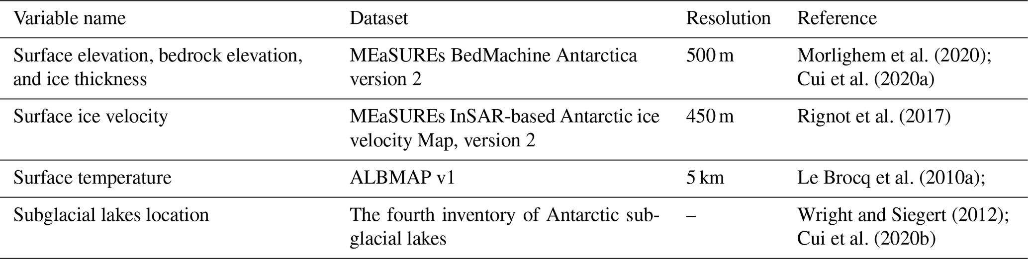
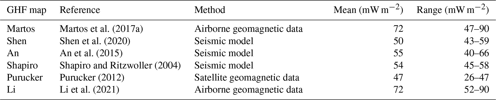
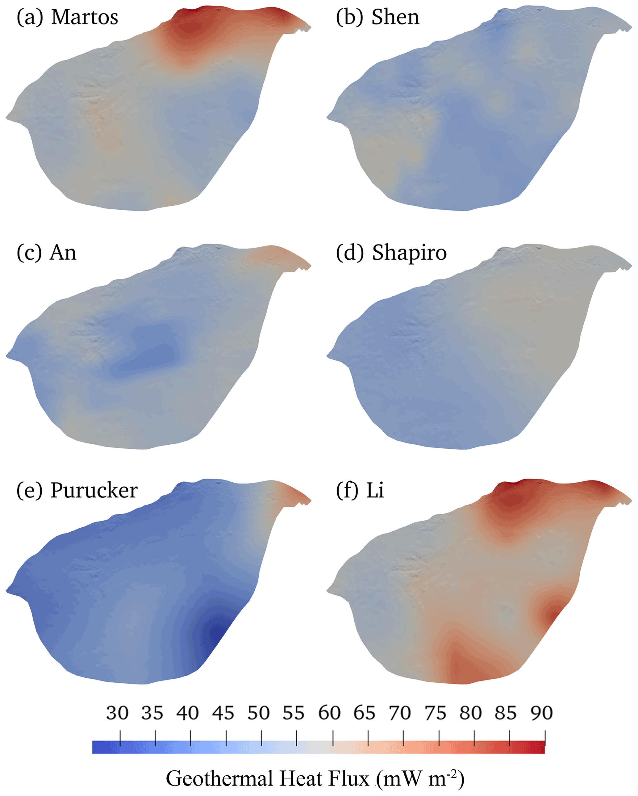
Figure 2 The spatial distribution of GHF over our domain, as described in Fig. 1. See Table 2 for the GHF map details.

3 Model

Our goal is to infer the basal thermal conditions, including basal temperature and basal melt rate, in the domain. Geothermal heat flux, englacial heat conduction, and basal friction heat are the main heat sources that determine the basal thermal conditions. Therefore, we need to model both ice flow velocity and stress for basal friction heat and ice temperature for englacial heat conduction.

We solve an inverse problem by a full Stokes model, implemented in Elmer/Ice, to infer the basal friction coefficient such that the modelled velocity best fits observations (Gagliardini et al., 2013). Using the best-fit basal friction coefficient, we obtain the ice flow velocity, stress, and basal friction heat. A proper initial vertical ice temperature profile subject to thermal boundary conditions is needed to solve the inverse problem. To obtain it, we use a forward model that consists of an improved shallow ice approximation (SIA) thermomechanical model with a subglacial hydrology model (Wolovick et al., 2021). The forward model uses the modelled velocity direction and basal slip ratio from the full Stokes inverse model to constrain its solution. We do steady-state simulations by coupling the forward and inverse models. We will describe the forward model in Sect. 3.1 and the inverse model in Sect. 3.2 and then the coupling in Sect. 3.3.

3.1 Forward model

The forward model consists of a thermomechanical steady state model using an improved shallow ice approximation (SIA) in equilibrium with the subglacial hydrological system (Wolovick et al., 2021). It has internal consistency between the following three components: ice flow, ice temperature, and basal water flux. The numerical model requires the following three coupled components to be consistent with one another: (1) integration for balance flux and englacial temperature downhill along the ice surface, (2) integration for basal water flux and freezing rate downhill in the hydraulic potential, and (3) rheology and shape function computations to determine the distribution of ice flux and shear heating. The model performs a fixed point iteration for consistency between these three components. In addition. we improve on the model used in Wolovick et al. (2021) by combining the observed velocity field, the velocity field from the full Stokes model, and the surface gradient direction to compute a merged surface flow direction field. The observations are used where flow is fast, Elmer/Ice modelled velocity is used where flow is slow, and the surface gradient is only used near the margins of the domain where the Elmer/Ice velocity field is not reliable (Fig. 3). The simulation is done on a finite difference mesh with resolution of 2.5 km.

The surface accumulation rate we used in the forward thermal model is the mean of Arthern et al. (2006) and Van de Berg et al. (2005). Both were accessed through the ALBMAP_v1 dataset (Le Brocq et al., 2010b).

One key complexity is how to deal with basal thermal boundary condition. At the bottom of ice shelves, we set basal temperature equal to the pressure melting point. At the bed of grounded ice, the boundary condition can be either a Dirichlet or Neumann condition, depending on the basal melting and subglacial water conditions. The basal boundary conditions are given by the following:

$$\begin{array}{}\text{(1)}& {\displaystyle }-k\left(T\right){\displaystyle \frac{\mathrm{d}T}{\mathrm{d}z}}=G,\text{for}T<T_{\mathrm{m}}\text{and}m=\mathrm{0};\text{(2)}& {\displaystyle }T=T_{\mathrm{m}},\text{for}m\ne \mathrm{0},\end{array}$$

where k(T) is the temperature-dependent thermal conductivity of ice, m is the basal melt rate, T_m is the pressure-dependent melting temperature, and G is GHF, taking the six GHF datasets listed in Table 2. The thermal condition will switch from Neumann (Eq. 1) to Dirichlet (Eq. 2) if the basal temperature exceeds the pressure-dependent melting point. The opposite switch from Dirichlet to Neumann is determined by the hydrology model if there is insufficient water input to supply a large freezing rate.

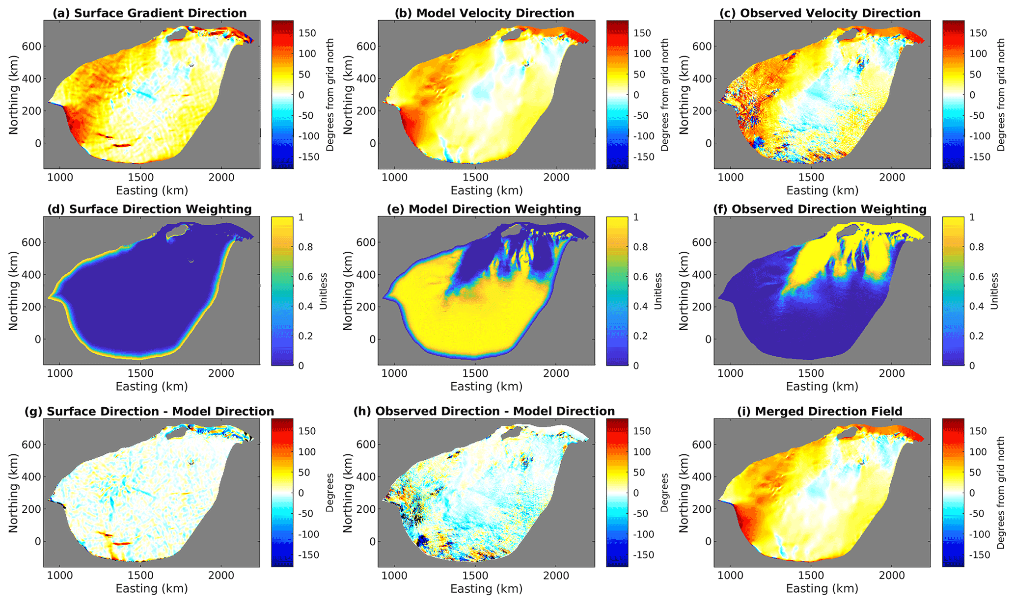
Figure 3 Surface velocity direction fields, in degrees clockwise from the grid north. The first row shows the direction from the surface gradient (a), Elmer/Ice modelled velocity (b), and the observed velocity direction (c). The middle row (d–f) shows the three corresponding weighting fields (the sum of these weights is 1). The bottom row shows the difference between the direction of surface gradient and Elmer/Ice modelled velocity (g), the difference between the observed velocity direction and Elmer/Ice modelled velocity (h), and the merged velocity field used in the forward model (i).

One improvement on the method from Wolovick et al. (2021) is that a temperate basal ice layer with non-zero thickness is permitted in our model in the case that the modelled basal ice temperature reaches the pressure melting point. We do this using a weak-form solution in which the volumetric englacial melt rate rises steeply as temperature exceeds the melting point. The englacial melting absorbs latent heat and serves to limit temperature rise. We parameterize the increase in volumetric melt rate as an exponential function of temperature with a 1 K e-folding temperature and a prefactor given by the englacial strain heating and the latent heat of fusion. All englacial meltwater generated this way is assumed to immediately drain to the bed.

Another key component of the forward model is the shape function determining the distribution of horizontal velocity with depth. We also improve the shape function in Wolovick et al. (2021) by including the basal slip ratio, ${\widehat{u}}_{\mathrm{b}}=u_{\mathrm{b}}/\stackrel{\mathrm{‾}}{u}$, where u_b is the basal velocity magnitude, and $\stackrel{\mathrm{‾}}{u}$ is the vertically averaged horizontal velocity magnitude. The slip ratio is taken from the full Stokes inverse model. Other than the addition of a spatially variable slip ratio, the shape function calculation is unchanged from Wolovick et al. (2021).

3.2 Inverse model with full Stokes model

The spatial distribution of basal friction in the domain is modelled by solving an inverse problem using the three-dimensional full Stokes model, Elmer/Ice, an open-source finite element method package (Gagliardini et al., 2013). The inverse model is based on adjusting the spatial distribution of the basal friction coefficient to minimize the misfit between simulated and observed surface velocities. The modelled velocity is obtained by solving the full Stokes equation, which includes conservation equations for both the momentum and mass of the ice, as follows:

$$\begin{array}{}\text{(3)}& {\displaystyle }\mathrm{\nabla }\cdot \mathit{\tau }-\mathrm{\nabla }p={\mathit{\rho }}_{\mathrm{i}}\mathit{g},\text{(4)}& {\displaystyle }\mathrm{\nabla }\cdot \mathit{v}=\mathrm{0},\end{array}$$

where τ​​​​​​​ is the deviatoric stress tensor, p is the isotropic pressure, ρ_i is ice density, g is the acceleration due to gravity (0, 0, −9.81) m s⁻², and v is ice velocity. According to Glen's flow relation, deviatoric stress is related to the strain rate tensor, $\dot{\mathit{\epsilon }}$, which can be described by $\mathit{\tau }=\mathrm{2}\mathit{\eta }\dot{\mathit{\epsilon }}$, where the effective viscosity of the ice, η, is sensitive to the temperature-dependent flow rate factor A(T) calculated using an Arrhenius equation (Cuffey and Paterson, 2010). The ice temperature distribution comes from the forward model in Sect. 3.1.

3.2.1 Mesh generation and refinement

First, we use Gmsh software (Geuzaine and Remacle, 2009) to generate an initial 2D horizontal footprint mesh with the boundary described in Sect. 2. Then we refine the mesh by an anisotropic mesh adaptation code called the Mmg library (http://www.mmgtools.org/, last access: 2 August 2022). The resulting mesh is shown in Fig. 4 and has minimum and maximum element sizes of approximately 1000 and 8000 m. The 2D mesh is then vertically extruded using 10 equally spaced, terrain-following layers.

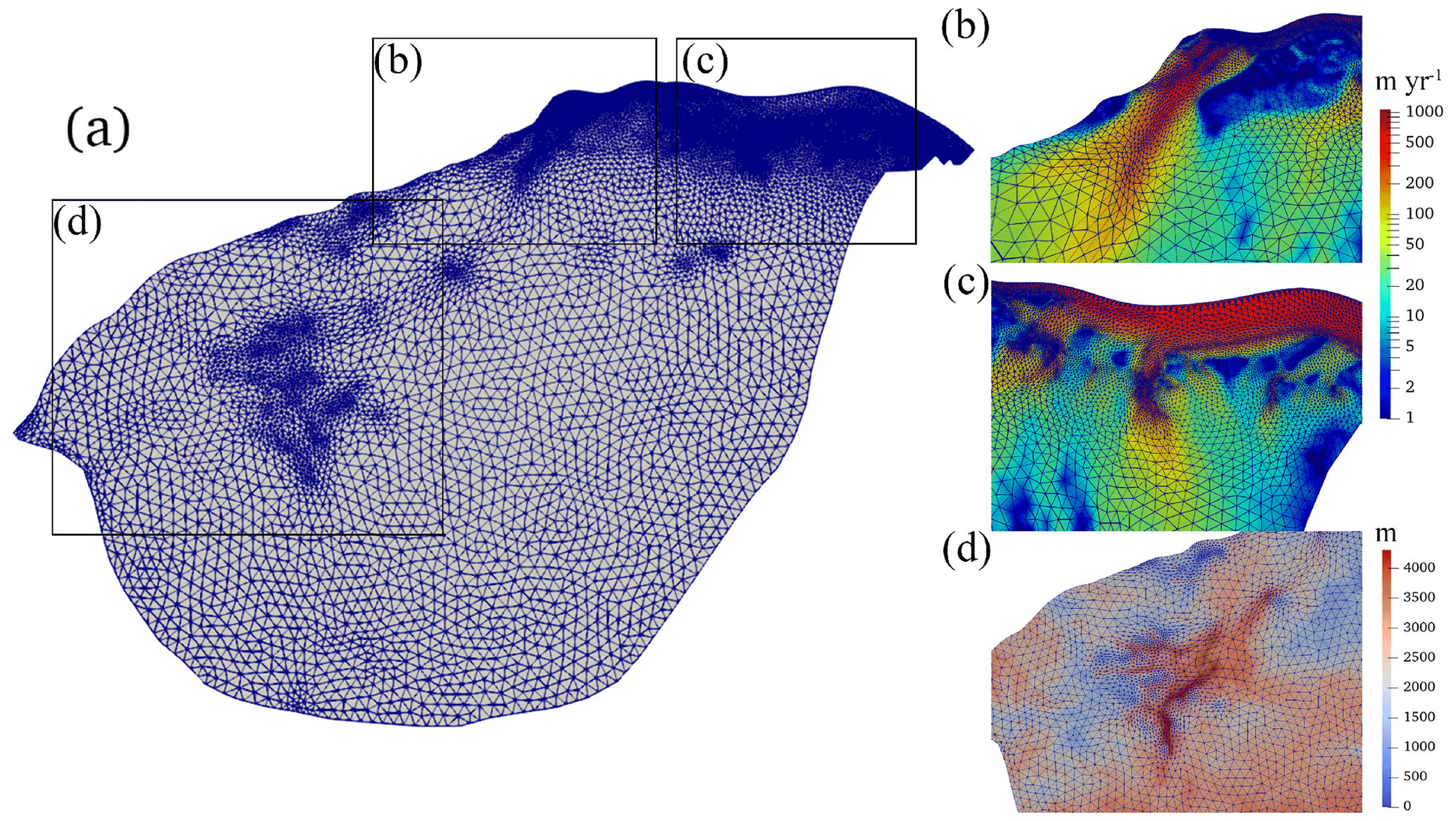
Figure 4 The refined 2D horizontal domain footprint mesh (a). Boxes outlined in panel (a) are shown in detail and overlain with surface ice velocity in panels (b) and (c) and with ice thickness in panel (d).

3.2.2 Boundary condition

The ice surface is assumed to be stress free. At the ice front, the normal stress under the sea surface is equal to the hydrostatic water pressure. On the lateral boundary, the normal stress is equal to the ice pressure applied by neighbouring glaciers and the normal velocity is assumed to be 0. The bed for grounded ice is assumed to be rigid, impenetrable, and fixed over time. Since we perform a stress balance snapshot in the full Stokes model, we do not need to prescribe surface mass balance or basal mass balance in the boundary conditions.

The normal basal velocity is set to 0 at the ice–bed interface. The linear sliding law is used to describes the relationship between the basal sliding velocity, u_b, and the basal shear force, τ_b, on the bottom of grounded ice, as follows:

$$\begin{array}{}\text{(5)}& {\mathit{\tau }}_{\mathrm{b}}=C{\mathit{u}}_{\mathrm{b}}.\end{array}$$

To avoid non-physical negative values, C=10^β is used in the simulation. We call β the basal friction coefficient rather than C. C is initialized to a constant value of 10⁻⁴ MPa m⁻¹ yr (Gillet-Chaulet et al., 2012) and then replaced with the inverted C in subsequent inversion steps.

3.2.3 Surface relaxation

We relax the free surface of the domain by a short transient run to reduce the non-physical spikes in initial surface geometry (Zhao et al., 2018). The transient simulation period here is 0.5 year, with a time step of 0.01 year.

3.2.4 Inversion and improvement for basal friction coefficient

Taking the results from the surface relaxation as our ice geometry, we use an inverse model to retrieve the basal friction coefficient, the deviatoric stress field, and ice velocity field. The inverse model adjusts the spatial distribution of the basal friction coefficient to minimize the value of the cost function (Morlighem et al., 2010), which is defined as the difference between the simulated surface velocity and the observed, as follows:

$$\begin{array}{}\text{(6)}& J_{\mathrm{0}}=\underset{{\mathrm{\Gamma }}_{\mathrm{s}}}{\int }{\displaystyle \frac{\mathrm{1}}{\mathrm{2}}}{\left(\mathrm{|}\mathit{u}\mathrm{|}-\mathrm{|}{\mathit{u}}_{\mathrm{obs}}\mathrm{|}\right)}^{\mathrm{2}}\mathrm{d}\mathrm{\Gamma },\end{array}$$

where Γ_s is the ice surface, and u and u_obs are the simulated and observed surface velocities.

To avoid over-fitting of the inversion solution to non-physical noise in the observations, the following regularization term,

$$\begin{array}{}\text{(7)}& J_{\mathrm{reg}}={\displaystyle \frac{\mathrm{1}}{\mathrm{2}}}{\int }_{{\mathrm{\Gamma }}_{\mathrm{s}}}\left({\left({\displaystyle \frac{\partial C}{\partial x}}\right)}^{\mathrm{2}}+{\left({\displaystyle \frac{\partial C}{\partial y}}\right)}^{\mathrm{2}}\right)\mathrm{d}\mathrm{\Gamma },\end{array}$$

is added to the cost function, and then the total cost function is defined as follows:

$$\begin{array}{}\text{(8)}& J_{\mathrm{tot}}=J_{\mathrm{0}}+\mathit{\lambda }{J}_{\mathrm{reg}},\end{array}$$

where λ is a positive regularization weighting parameter. An L-curve analysis (Hansen, 2001) has been carried out for inversions to find the optimal λ by plotting the term J_reg as the function of J₀. The optimal value of 10¹⁰ is chosen for λ to minimize J₀.

Basal friction in reality depends on basal temperature, i.e. it is relatively large on cold beds, since the ice is frozen, and small on warm beds, where the basal temperature reaches the pressure melting point, allowing the ice to slide (Greve and Blatter, 2009). However, in the inverse model, the basal friction coefficient (Eq. 5) is adjusted to match velocity observations without regard to basal temperature, which leads to unrealistic noise manifested as local spikes in modelled basal friction heat (Fig. 5a).

We improve the parameterization of β via C in Eq. (5) (Sect. 3.2.2) by considering basal temperature T_bed, as follows:

$$\begin{array}{}\text{(9)}& {\mathit{\beta }}_{\mathrm{new}}={\mathit{\beta }}_{\mathrm{old}}+\mathit{\alpha }\left(T_{\mathrm{m}}-T_{\mathrm{bed}}\right),\end{array}$$

where β_old is from the inverse model, α is a positive factor to be tuned, and T_m is the pressure-dependent melting temperature. β_new equals β_old at a bed with temperate ice and is larger than β_old at a bed with ice temperature lower than T_m. We tune α in the range of [0.1, 2], with an interval of 0.1, and find that the local spikes in modelled friction heat become fewer (Fig. 5) as α increases from 0.1 to 1 but stay almost constant with α from 1 to 2. Therefore, we take α to be 1 and use the parameterization of β_new in Eq. (5) in all the simulations. Using Eq. (9), the difference in the simulated and observed surface velocity is unchanged over the region, except for some parts of the inland boundary.

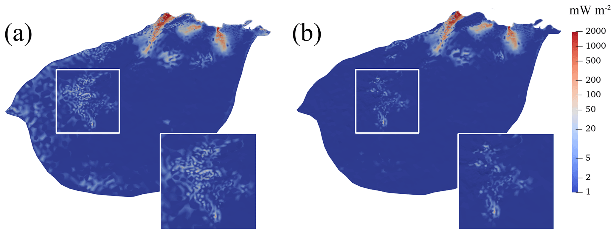
Figure 5 Comparison of modelled basal friction heat with basal friction coefficient β_old (a) and β_new with α=1 (b), as driven by Martos et al. (2017) GHF. The white square is enlarged.

3.2.5 Basal melt rate

Based on the inverted basal velocity and basal shear stress, we can calculate the basal friction heat. We then produce the basal melt rate using the thermal equilibrium, as follows (Greve and Blatter, 2009):

$$\begin{array}{}\text{(10)}& M={\displaystyle \frac{G+{\mathit{u}}_{\mathrm{b}}{\mathit{\tau }}_{\mathrm{b}}+k\left(T\right)\frac{\mathrm{d}T}{\mathrm{d}z}}{{\mathit{\rho }}_{\mathrm{i}}L}},\end{array}$$

where M is the basal melt rate, G is GHF, u_bτ_b is the basal friction heat, $-k\left(T\right)\frac{\mathrm{d}T}{\mathrm{d}z}$ is the upward heat conduction, ρ_i is the ice density, and L is the latent heat of ice melt. Geothermal heat and frictional heating from basal slip warm the base, while the upward heat conduction to the interior cools the base. Note that the basal melt rate can be either positive (melting) or negative (freezing), depending on the heat balance.

3.3 Experimental design of coupled simulations

We design the coupled simulations in an eight-step scheme for coupling the forward model and inverse model, similar to Zhao et al. (2018):

1. We run the forward model with the velocity direction taken from a mixture of the surface gradient and surface velocity observations and obtain an initial modelled englacial temperature (Fig. 3).

2. We do surface relaxation in Elmer/Ice with the englacial temperature from step 1.

3. Taking the results from step 2 as the initial state, we do an inversion in Elmer/Ice, using the modelled englacial temperature from step 1, to obtain a modelled surface velocity best fit to the observed surface velocity. The modelled surface velocity will remove some artefacts in the observed field.

4. We run the forward model using the velocity directions derived by merging the Elmer/Ice modelled velocity, the surface gradient, and the surface velocity observations (Fig. 3). We use the modelled velocity from the full Stokes inverse model to constrain the basal slip ratio, then constrain the rheology and shape function in the forward model. Then we obtain an updated modelled englacial temperature.

5. We run the inverse model in Elmer/Ice with the improved englacial temperature from step 4 and obtain an updated modelled velocity.

6. We run the forward model again using the ratio of basal sliding to column-averaged velocity in Elmer/Ice from step 5 to constrain the slip ratio and obtain a further updated basal temperature.

7. We run the inverse model again in Elmer/Ice with the improved englacial temperature from step 6 and obtain an updated modelled velocity and stress.

8. We analyse the modelled results in step 7 and calculate basal friction heat and basal melt rate.

We perform the above procedure for all six sets of GHF to produce six different results for the basal thermal conditions.

4 Simulation results

4.1 Ice velocity

In the inverse model, the misfit between the modelled and the observed surface velocity is minimized. Therefore, we obtain very similar distributions of modelled surface velocity field using different GHF maps. Figure 6 shows the modelled velocity in the experiment, using the Martos et al. (2017) GHF as an example. The modelled surface velocity shows spatial similarities to the observed surface velocity (Fig. 6a, b). In total, three fast-flowing outlet glaciers (Lambert, Lepekhin, and Kronshtadtskiy glaciers) deliver ice to the ice shelf. The velocity of the Lambert Glacier exceeds 800 m yr⁻¹ at the grounding line. The Lepekhin Glacier and the Kronshtadtskiy Glacier have maximum flow velocities of about 200 and 400 m yr⁻¹ at their grounding lines, respectively. Regions with large differences between modelled and observed surface velocity occupy a small fraction of the whole area (Fig. 6c) and are associated with high-velocity gradients. Ice velocity decreases with depth. Figure 6c shows the modelled basal ice velocity. The maximum basal velocity on the Lambert Glacier exceeds 500 m yr⁻¹ near the grounding line, and maximum basal velocities on Lepekhin Glacier and the Kronshtadtskiy Glacier reach about 150 and 200 m yr⁻¹ at the grounding line.

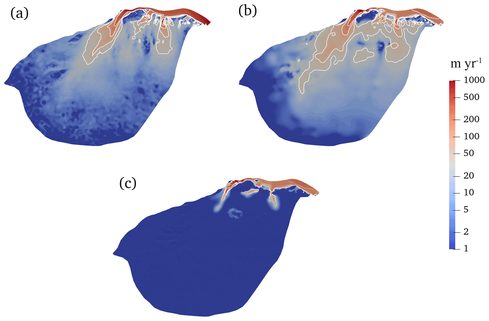
Figure 6 (a) Observed surface velocity, (b) modelled surface velocity in the experiment, using the Martos et al. (2017) GHF, and (c) modelled basal velocity. The white solid lines in panels (a), (b), and (c) represent speed contours of 30, 50, 100, and 200 m yr⁻¹, respectively. The three fast-flowing outlet glaciers in panel (a) from left to right are the Lambert, Lepekhin, and Kronshtadtskiy glaciers.

4.2 Basal ice temperature and heat conduction

In Fig. 7, we show the modelled basal temperature from the six experiments. The modelled ice basal temperatures in the fast-flowing regions are all at the pressure melting point (warm). However, there are significant differences in the modelled distribution of warm-based conditions in the slow-flowing region using different GHF maps. The basal temperature is highly dependent on the GHF. In the experiment using Li et al. (2021) GHF (Fig. 7f), which has the highest GHF within the domain, the basal temperature is at the melting point over most of the domain, with extensive cold-based regions confined to the southern part. The experiment using the Martos et al. (2017) GHF (Fig. 7a), which has the second highest GHF, yields the second-largest area of a warm base, and the experiment using Purucker (2012) GHF (Fig. 7e), with the lowest GHF, gives the smallest warm-based area which is concentrated around the fast-flowing ice. All experiments display cold basal temperatures to the southwest of the Lambert Glacier basin, which is associated with thin ice over subglacial mountains (Fig. 1c).

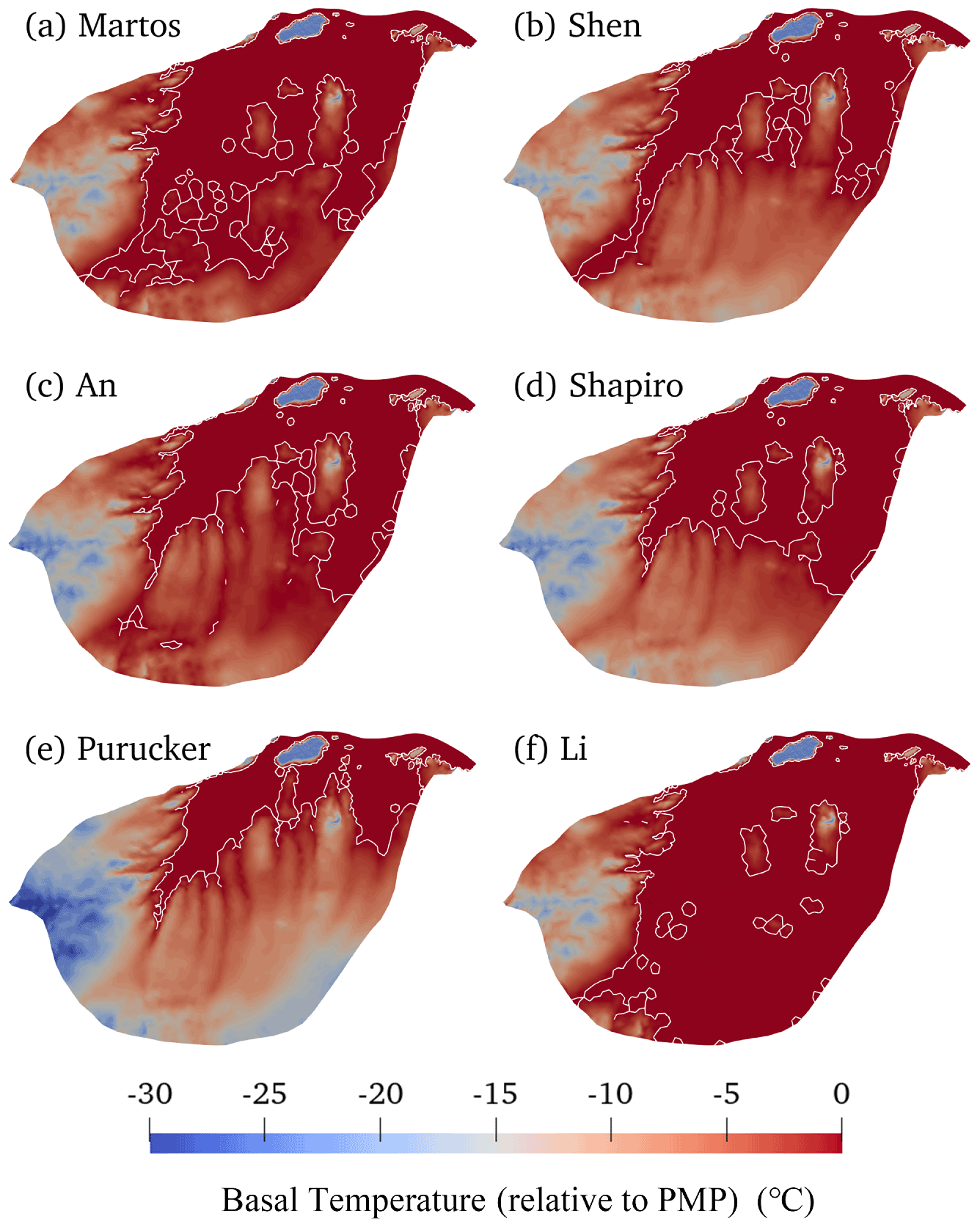
Figure 7 Modelled basal temperature relative to pressure melting point, in panels (a) to (f), corresponding to the GHF in panels (a) to (f) in Fig. 2. The ice bottom at the pressure melting point is delineated by a white contour.

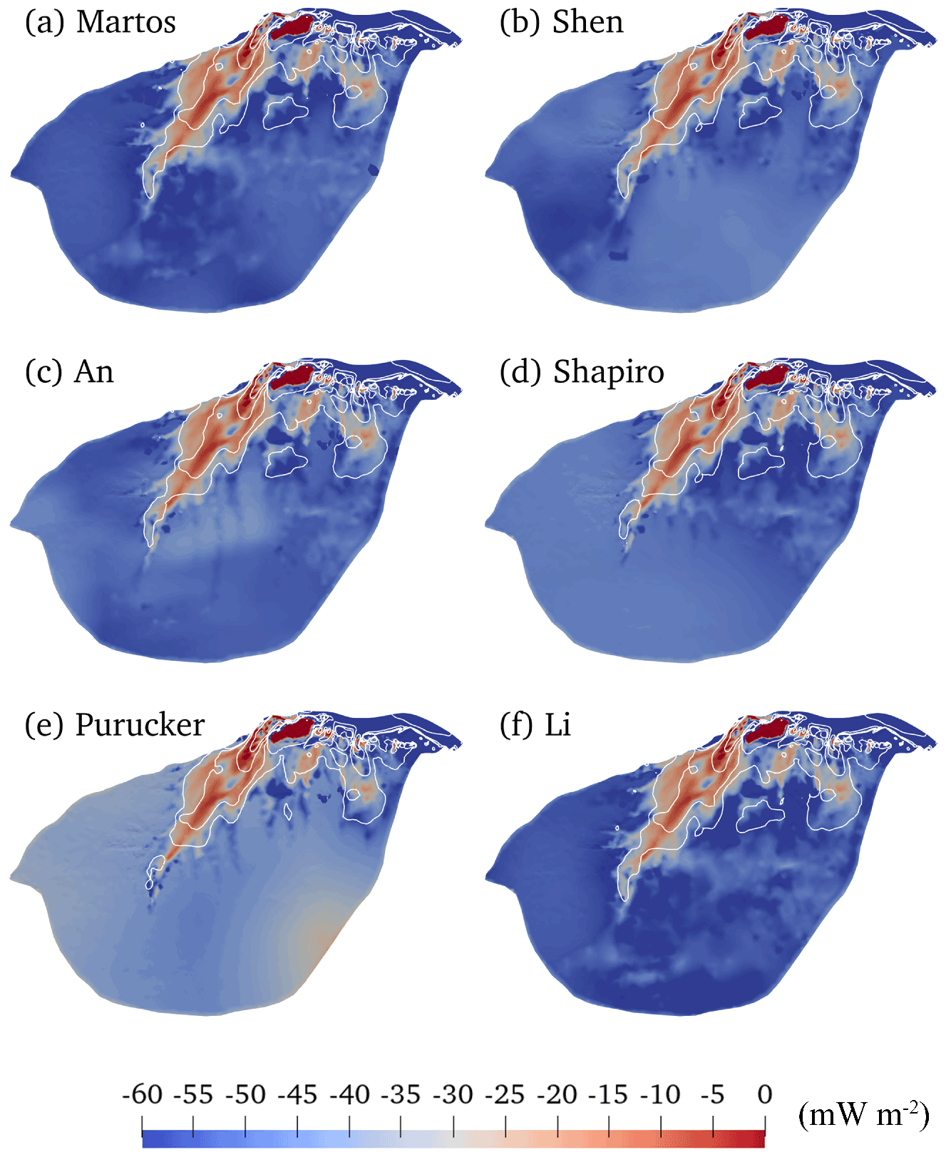
Figure 8 Modelled heat change in basal ice by upward englacial heat conduction (mW m⁻²). The negative sign means that the upward englacial heat conduction causes heat loss from the basal ice, as defined by the colour bar with cooler colours representing more intense heat loss by conduction. Panels (a) to (f) correspond to the GHF in panels (a) to (f) in Fig. 2. The white solid curves represent modelled speed contours of 30, 50, 100, and 200 m yr⁻¹, which is the same as in Fig. 6b.

Figure 8 shows the modelled heat change of basal ice by upward englacial heat conduction in the six experiments. In most regions of the fast-flowing tributaries with velocity higher than 30 m yr⁻¹, the heat loss caused by upward basal heat conduction is lower than 30 mW m⁻² in all experiments, reflecting the development of a temperate basal layer that limits the basal thermal gradient. For the vast inland areas, experiments yield heat loss by upward heat conduction in the range of 45–60 mW m⁻², except for the experiment driven by the Purucker (2012) GHF, which has lower values around 30–45 mW m⁻². This is because the upward heat conduction equals GHF where the basal temperature is below the pressure melting point, and the Purucker (2012) GHF is lower than the others.

4.3 Basal friction heat

There is no significant difference in modelled basal friction heat across these six experiments, reflecting the fact that all of them have been tuned to match the surface velocity observations. So, we show only the modelled basal friction driven by the Martos et al. (2017) GHF (Fig. 5b). As expected, basal friction heat is high in fast-flowing regions. The three fast-flowing tributaries have friction heat amounting to more than 50 mW m⁻², with the Lambert and Kronshtadtskiy glaciers having 2000 mW m⁻² at the grounding line.

4.4 Basal melt rate

We obtain the basal melt rate using the thermal balance equation (Eq. 10). Figure 9 shows the modelled basal melt rate in the six experiments using different GHF maps. Regions with the basal melt rate coincide with a warm base where basal temperatures reach the pressure melting point. There are significant differences in the area of basal melting among the six experiments due to the large variability in GHF. The experiments using the Li et al. (2021) and Martos et al. (2017) GHF yield the largest area with basal melting. In contrast, the experiment using the Purucker (2012) GHF gives the least area with basal melting (Fig. 9).

The modelled basal melt rate is below 5 mm yr⁻¹ in the parts of the vast inland region that are warm based. Higher basal melt rates occur in fast-flowing regions (Fig. 9) where frictional heat is high (Fig. 5b), despite the differences in GHF (Fig. 2). Basal melt rate is above 10 mm yr⁻¹ near the grounding line, reaching 500 mm yr⁻¹ at the grounding line of the central flowline running onto the Amery Ice Shelf. Thus, in fast-flowing regions, frictional heat is the dominant factor rather than GHF, consistent with Larour et al. (2012), who noted that slower-flowing ice in the interior of the ice sheet will be more sensitive to the GHF, but frictional heat dominates GHF in regions of fast ice flow. We use the positions of observed subglacial lakes to validate simulated regions with basal melting (Fig. 9). The modelled warm base in the experiment using Li et al. (2021) GHF covers all the observed subglacial lakes in the domain (Fig. 9f), including the recently discovered second-largest subglacial lake in Antarctica (Cui et al., 2020b). The warm base in the experiment using the Martos et al. (2017) GHF covers the second greatest number of observed subglacial lakes (Fig. 9a), and the experiment using the An et al. (2015) GHF covers the third (Fig. 9c). The experiment using the Shen et al. (2020) GHF captures two subglacial lakes in the southwest of the domain (Fig. 9b), while the experiment using the Shapiro and Ritzwoller (2004) GHF missed many known subglacial lakes in the southwest of the domain but successfully captures the recently discovered second-largest subglacial lake (Fig. 9d). The experiment using the Purucker (2012) GHF performs worst in recovering subglacial lake locations (Fig. 9e).

There are localized negative values of basal melt rate, indicating basal refreezing at three locations (Fig. 9). The modelled refreezing locations are generally characterized by large gradients in ice thickness, typically thinning by 700 m across a distance of 2 km. Radar surveys have not yet been carried out to confirm these freeze-on locations.

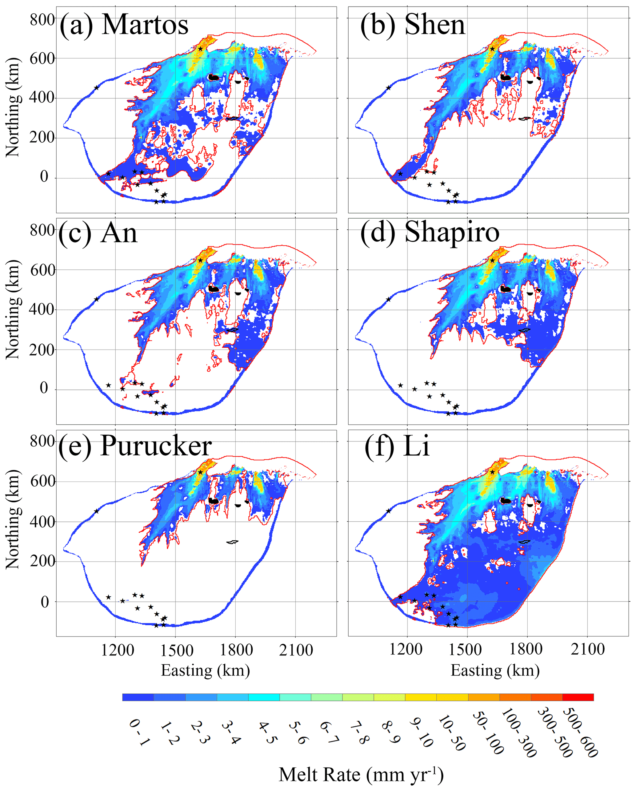
Figure 9 Modelled basal melt rate (mm yr⁻¹) in panels (a) to (f) correspond to the GHF in panels (a) to (f) in Fig. 2. The ice bottom at pressure melting point is surrounded by a red contour. The stars denote the locations of observed subglacial lakes, and the area surrounded by the black line is the likely second largest subglacial lake in Antarctica. There is modelled basal refreezing at three local places painted in black.

5 Discussion

Uncertainties and bias in our simulations can come from several sources. We expect that the present-day accumulation rate field in our modelling will be higher than the long-term average because of a lower accumulation rate during glacial periods (Watanabe et al., 2003; Van Ommen et al., 2004). This will tend to increase the downward advection of cold ice in our model, lowering the basal temperature in comparison to reality. On the other hand, we also expect that the modern-day surface temperature in our modelling will be higher than the long-term average temperature, again because of lower temperatures during glacial periods. This will tend to increase our modelled basal temperature in comparison with reality. It is unclear which of these competing biases is stronger.

Subglacial topography has an influence on geothermal heat at kilometre scales. Typically, it has been assumed that subglacial ridges receive less heat flow and subglacial valleys receive more heat flow, in comparison to the regional average (e.g. van der Veen et al., 2007; Colgan et al., 2021). However, the effect depends on subglacial rock type. Heat tends to follow the path of least resistance to the surface. The thermal conductivity of rock varies with lithology and can be either greater or smaller than the thermal conductivity of ice (Willcocks and Hasterok, 2019); thus, the sign of the topographic effect on GHF can be either negative or positive. Without knowing a priori whether the topographic effect will be positive or negative, it is hard to apply a topographic correction field to the GHF input field.

GHF distribution largely governs basal thermal conditions. Many previous studies (Larour et al., 2012; Pattyn, 2010; Pittard et al., 2016; Van Liefferinge and Pattyn, 2013; Van Liefferinge et al., 2018) on basal temperature and basal melt have used the Shapiro and Ritzwoller (2004), Fox Maule et al. (2005), Purucker (2012), and An et al. (2015) GHF datasets, with a few making use of the more recent Martos et al. (2017) and Li et al. (2021) GHF datasets. In this study, we find that the Li et al. (2021) and Martos et al. (2017) GHF datasets have higher GHF than the earlier datasets in the Lambert–Amery domain and consequently have the largest area with a warm base. The warmer basal conditions best match the observed distribution of subglacial lakes. However, it should be noted that observations of subglacial lakes are a one-sided constraint. A model result that does not predict basal melt at the location of the observed lakes is clearly too cold at that location. But if the model result shows basal melt at a place with no observed lakes, it is not clear whether this is because the model is too warm, the subglacial water exists in a form other than ponded lakes, or that lakes are present, but we do not have the data to detect them.

A lake complex beneath the Devon Island ice cap in Canada exists at temperatures well below pressure melting point due to large concentrations of dissolved salts (Rutishauser et al., 2018), and no similar ones are known to exist beneath the Antarctic ice sheet. Furthermore, relatively high electrical conductivity beds such as clay-rich sediments surrounded by bedrock can give rise to false positives in radar detections of subglacial water bodies (Tulaczyk and Foley, 2020​​​​​​​).

Our simulations make improvements on previous approaches. We use the full Stokes flow model in the inversion of basal friction field rather than a simplified physics model as in Wolovick et al. (2021). We also improve on the treatment of the basal friction field by imposing a larger basal friction where the ice bottom is colder than the pressure melting point and which increases with the temperature difference from freezing point. These modifications produce more physically meaningful results, since we expect frozen beds to have high basal friction. Hence, the basal friction field is constrained by simulated temperatures in addition to producing the best fitting match of simulated and observed surface velocities.

Van Liefferinge and Pattyn (2013) estimated basal temperature for the Antarctic ice sheet using three GHF datasets (Fox Maule et al., 2005; Shapiro and Ritzwoller, 2004; Purucker, 2012), and each of the datasets were improved by the method in Pattyn (2010). Their modelled temperatures show spatial similarities to our experiment field using the Purucker (2012) GHF. Pittard et al. (2016) did sensitivity experiments of the Lambert–Amery glacial system based on three GHF fields (Fox Maule et al., 2005; An et al., 2015; Shapiro and Ritzwoller, 2004), using the Parallel Ice Sheet Model (PISM), and found that modelled basal temperature reached the pressure melting point only under the fast-flowing ice, with maximum melting rates of 500 mm yr⁻¹ at places very close to the grounding line of the central flowline onto the Amery Ice Shelf. We also model maximum basal melt at similar locations in the six GHF experiments. However, the Pittard et al. (2016) region of basal melt is mainly confined to the Lambert Glacier tributary and matches only that of our experiment using Purucker (2012) GHF.

We analyse the contribution of GHF and frictional heat to basal melt. The basal friction is a significant heat sources only under fast-flowing ice. Most GHF distributions (except Martos et al., 2017, and Li et al., 2021) in the grounded ice sheet near the ice shelf are homogeneous, but frictional heating in the fast-flowing ice is more than 10 times higher than that in the slow-flowing ice. Thus slower-flowing ice in the interior of the ice sheet is more sensitive to the GHF than fast-flowing ice (Larour et al., 2012).

GHF has its largest impact on the basal melt of the inland ice sheet. There are two principle ways to constrain GHF, i.e. (1) direct measurement and (2) inversion by multiple geophysical methods. The GHFs used in this study are based on the inversion of satellite or aeromagnetic data and seismic tomography. Direct observations of heat flux are difficult to obtain in Antarctica, and satellite data are low resolution. The most efficient method is to invert the heat flux through aerial geomagnetic observation such as for the Martos and Li GHF fields (Martos et al., 2017; Li et al., 2021). However, there are still large data gaps in remote regions, especially in PEL, leaving just inversion using satellite magnetic data with a lower resolution. The Li et al. (2021) field uses the latest aeromagnetic data to estimate the GHF in the PEL region, and this gives higher values than derived previously.

To validate the modelled basal melt, we use the locations of detected subglacial lakes. There may be many other undiscovered subglacial lakes beneath the study area, and further discoveries would help us validate the model results and possibly refine GHF maps. In addition, further observational constraints with a two-sided sensitivity to ice temperature, such as observations of subglacial freeze-on or measurements of englacial attenuation, would help us to identify areas in which the GHF maps are too warm, in addition to those areas in which they are too cold.

6 Conclusions

In this paper, we estimate the basal thermal conditions of the Lambert–Amery system by coupling a forward model and an inverse model, based on six different GHF datasets. We analyse the contribution of GHF, heat conduction, and basal friction to the modelled basal melt rate. We verify the result using the locations of all known subglacial lakes and evaluate the reliability of six GHF datasets in our study domain.

Our approach is distinct from that used to find GHF fields employed by Wolovick et al. (2021); in particular, the use of a full Stokes model allows the method to be extended to fast-flowing ice streams and ice shelf domains where neither the shallow ice nor shallow shelf approximations are valid. We also improve the basal friction calculation to include information on the basal ice temperature relative to its pressure melting point. This procedure results in removal of unrealistic noise manifested as local spikes in modelled basal friction heat.

We find significant differences in the spatial extent of temperate ice in the slow-flowing areas among the six experiments due to large variability in GHF. The experiments using the Li et al. (2021) and the Martos et al. (2017) GHF yield the largest area with basal melting and match the subglacial lake locations best. In contrast, the experiments using the Purucker (2012) GHF give the least area with basal melting and the worst match with subglacial lake locations. We suggest that the GHF datasets from Li et al. (2021) and Martos et al. (2017) are the most suitable choice for this study region. We cannot make our own GHF map from our analysis. While we can pick the GHF in places where the Li and Martos geothermal heat flow maps (Li et al., 2021; Martos et al., 2017) are consistent and both agree with the observations, we do not know which (if either) are correct where the Li and Martos GHF datasets disagree, and there are no observations. In order to make this determination, we would need additional observational constraints on the basal thermal state, such as measured basal temperatures from deep ice cores or observed refreeze-on, but neither are available in the region.

The fast-flowing region has fast basal velocities and high frictional heat, but there are large differences in basal melting rates between the six GHF datasets. The fast-flowing tributaries have frictional heating in the range of 50–2000 mW m⁻². In the vast inland areas, our experiments generally yield high upward heat conduction in the range of 45–60 mW m⁻², which means that GHF dominates the heat content of the basal ice in the slow flow regions. The modelled basal melt rate reaches 50–500 mm yr⁻¹ locally in three very fast flow tributaries (Lambert, Lepekhin, and Kronshtadtskiy glaciers) feeding the Amery Ice Shelf and is in the range of 0–5 mm yr⁻¹ in the inland region.