Brief communication: Unravelling the composition and microstructure of a permafrost core using X-ray computed tomography

The microstructure of permafrost ground contains clues to its formation and hence its preconditioning to future change. We applied X-ray computed microtomography (CT) to obtain high-resolution data (Δx=50 µm) of the composition of a 164 cm long permafrost core drilled in a Yedoma upland in north-eastern Siberia. The CT analysis allowed the microstructures to be directly mapped and volumetric contents of excess ice, gas inclusions, and two distinct sediment types to be quantified. Using laboratory measurements of coarsely resolved core samples, we statistically estimated the composition of the sediment types and used it to indirectly quantify volumetric contents of pore ice, organic matter, and mineral material along the core. We conclude that CT is a promising method for obtaining physical properties of permafrost cores which opens novel research potentials.

1 Introduction

Arctic permafrost ground contains considerable amounts of ground ice and organic matter. Melting of excess ice – ground ice which exceeds the volume of the pore space that the sediment would have under natural unfrozen conditions – leads to ground subsidence and thermokarst formation, thereby affecting Arctic ecosystems (Kokelj and Jorgenson, 2013) and increasing the risk of infrastructure failure (Schneider von Deimling et al., 2021). Thawing and subsequent decomposition of organic matter can increase greenhouse gas release in Arctic lowlands, potentially causing a positive climate feedback (Schuur et al., 2015). Hence, an accurate quantification of the amounts and the distribution of both ground ice and organic matter in permafrost ground is needed in various realms of permafrost research, for example, to improve carbon stock assessments (Strauss et al., 2017) and model projections of permafrost thaw (Nitzbon et al., 2020). In addition to excess ice and organic matter, the structure and contents of other permafrost constituents such as pore ice, gas inclusions, and mineral grains are also of interest, as they affect material properties and provide additional insights into the processes that formed the soil. Permafrost composition and the cryostructure at a given site typically are characterized through visual description of exposures or drill cores from a given site (e.g. Kanevskiy et al., 2011). A quantitative determination of the composition of permafrost is then approached by sub-sampling exposures or cores along the direction of deposition and eventually measuring ground ice, organic carbon, and mineral contents through laboratory analyses of the samples (e.g. Schirrmeister et al., 2011). However, this approach is destructive, has a low stratigraphic resolution on the order of 1 to 5 cm for cores and even lower for exposures, and does not provide information on the spatial configuration and microstructure of the samples' constituents. Furthermore, measuring gas contents and distinguishing excess ice from pore ice are very inaccurate using these classical analysis techniques.

Following pioneering work to investigate snow properties (Coléou et al., 2001; Schneebeli and Sokratov, 2004), in recent years microstructure analysis with X-ray computed tomography (CT) has turned into a standard method in various geoscience disciplines like soil science, stratigraphy, or glaciology (Cnudde and Boone, 2013; Withers et al., 2021; Oggier and Eicken, 2022). Across disciplines, the general aim of non-invasive imaging like CT is to deduce functional behaviour or process understanding at larger scales through mapping of the microscale composition and morphology of all constituents in a sample (Cnudde and Boone, 2013). Despite the broad potential for applications which require in-depth knowledge of the composition and physical properties of permafrost, there are only few reports of CT being applied to study frozen soil samples (Torrance et al., 2008). Calmels and Allard (2004) pioneered the use of CT to measure excess ice and gas contents in ice-rich permafrost of a lithalsa landform. Calmels and Allard (2008) built on this and used CT scans to establish links between various permafrost landforms and microscale cryostructures. CT scans have further been used to study ground ice structures and periglacial processes in Arctic (Calmels et al., 2008, 2010, 2012) and Antarctic (Lapalme et al., 2017) permafrost. More recently, Romanenko et al. (2017) and Rooney et al. (2022) used CT imaging to investigate dynamic changes in the pore space due to freezing and thawing.

However, we are not aware of any studies that aimed at a detailed quantification of the constituents of permafrost drill cores, in particular including a distinction between all major constituents of permafrost soils as a porous composite material: excess ice, pore ice, organic matter, mineral grains, and gas inclusions. Moreover, a systematic quantitative comparison between the laboratory-measured and the CT-derived composition of permafrost cores has not been done to date.

In the present study, we use CT imaging to investigate a permafrost drill core from a Yedoma upland in north-eastern Siberia. Specifically, we assess the suitability of CT imaging and image processing methods to quantify vertical profiles of the volumetric contents as well as the structures of gas, excess ice, pore ice, organic matter, and mineral constituents. We further use laboratory measurements of total ice, organic matter, and mineral contents to evaluate and complement the CT analysis with the overall goal to obtain a detailed high-resolution (50 µm) three-dimensional composition of the entire permafrost core. With our work we propose a methodological advancement in employing CT imaging for the measurement of volumetric contents and structures of all major constituents of permafrost as a porous composite material, which opens potential for further research on microstructure and physical properties.

2 Methods

2.1 Field site and coring

The permafrost core analysed in this work was sampled from an ice-rich Yedoma permafrost upland plateau on Kurungnakh Island, Lena River delta, north-eastern Siberia (72.36613^∘ N, 126.27272^∘ E). Kurungnakh Island is the easternmost portion of the structurally elevated western Lena River delta and rises up to 55 m above sea level. The core was obtained during the field campaign in September 2017. A soil pit was excavated to the maximum thaw depth of 20 cm followed by drilling and coring of the frozen material underneath to a depth of 164 cm. The diameter of the frozen core was 7.5 cm. The frozen core pieces were wrapped in a thin plastic sheet, labelled individually at the field site, and stored in the freezers at the nearby Samoylov research station. The core samples were shipped in frozen condition to AWI Potsdam's laboratory during autumn 2017. The samples were kept frozen until further analysis.

2.2 CT analysis of the entire core

2.2.1 Scanning

The permafrost core was scanned in February 2019 at the Helmholtz Centre for Environmental Research (UFZ) in Halle. First, the permafrost core was assembled in segments up to about 30 cm long, each of which fit into the X-ray CT chamber. The cores were kept frozen until image acquisition and shielded with bubble wrap during the imaging process. Scanning was conducted with an X-ray microtomography system (Nikon Metrology, XT H 225) with settings adjusted to 150 kV, 320 µA, and 500 ms exposure time and a 0.5 mm copper filter for beam hardening reduction. A total of 2748 projections were acquired during a full rotation, with 1 frame per projection. The core segments were scanned in two vertical steps (top, bottom) with sufficient overlap to put the two tomograms together afterwards. The total scan time for one segment amounted to about 23 min during which ice melting was negligible. Finally, the radiographs were reconstructed into a 3D tomogram with a voxel size of 50 µm and 8 bit greyscale resolution using the CT Pro 3D software by Nikon Metrology. The greyscale range of each CT scan was normalized by setting the darkest and brightest 0.2 percentile to 0 and 255, respectively.

2.2.2 Image preprocessing

Image preprocessing (along with image analysis and segmentation) was applied to the whole core length of 164 cm and consisted of four steps, all of which were done using ImageJ/FIJI (Schindelin et al., 2012). First, cylindrical regions of interest (ROIs) were determined for each segment, which were fully within the core diameter without extending beyond its uneven boundaries. Second, depth intervals with artefacts, e.g. due to cracks in the core that occurred during the drilling process, were identified visually in order to exclude them from quantitative analysis. Third, overlaps between adjacent scans were removed manually by identifying identical horizontal slices in both images. Lastly, image noise was removed by applying three consecutive 2D non-local means filtering steps, one in each principal direction. The filter settings (noise standard deviation =6, smoothing factor =1) were adjusted to the noise level in the raw images, which resulted from the relatively short scan time that was necessary to reduce melting in the X-ray CT chamber. This denoising procedure, which is equivalent to a single 3D non-local means filtering step with a noise standard deviation of 18, is known to be superior to more conventional denoising filters in that it preserves edges while efficiently removing noise in homogeneous areas (Schlüter et al., 2014).

2.2.3 Image segmentation

Visual inspection of the data indicated that the cores contained four material classes, which could clearly be separated by their distinct peaks in the histograms of greyscale values. These were (from dark to bright) gas-filled pores, excess ice, and two mixed sediment types of unknown composition denoted as types A and B. Manual threshold detection with adjustments for different illumination and different numbers of material classes in individual segments resulted in robust segmentation results which were checked by visual inspection (Fig. 1).

2.3 Laboratory analysis of core samples

In August 2020, the frozen core was prepared for further lab analysis in the cold laboratory (below 0 ^∘C temperature). First, all samples were photographed and visually described. Then, the core was cut into smaller sections. All surfaces and saw blades were cleaned with ethanol before and during the cutting. A total of N_j=66 sub-samples were obtained with a core disc thickness ranging between 0.9 and 1.9 cm, each associated with a central depth z_j. The volume V_j and weight m_wet,j of all frozen sub-samples were measured. The samples were then allowed to thaw and then dried in an oven at a temperature of 100 ^∘C for 24 h. The total ice loss was then determined by subtracting the dry weight from the wet weight of the sample: $m_{\mathrm{i}}=m_{\text{wet}}-m_{\text{dry}}$. Then, the volumetric total ice content (θ_i(z_j)) was calculated as

$$\begin{array}{}\text{(1)}& {\mathit{\theta }}_{\mathrm{i}}\left(z_j\right)=m_{\text{i},j}/\left({\mathit{\rho }}_{\mathrm{i}}{V}_j\right),\end{array}$$

with ρ_i=916 kg m⁻³ being the density of ice.

The remaining dried sediment samples (grain size fraction <2 mm) were homogenized and analysed for the total organic carbon (TOC) content using standard laboratory procedures. The grain size fraction >2 mm was zero, which is characteristic for the predominantly silty material of the Yedoma deposits. The gravimetric TOC content (g_TOC) was measured twice with a vario MAX C analyser after carbonate was removed by adding hydrochloric acid (4 %). For a valid comparison between the laboratory and CT data, we converted the TOC contents into contents of (intact) organic matter. For this, the TOC contents were multiplied with the adapted van Bemmelen factor of f_vB=2 suggested by Pribyl (2010). The volumetric organic matter content (θ_o(z_j)) was then calculated for each sample j=1…N_j as

$$\begin{array}{}\text{(2)}& {\mathit{\theta }}_{\text{o}}\left(z_j\right)=f_{\text{vB}}{g}_{\text{TOC},j}{m}_{\text{dry},j}/\left({\mathit{\rho }}_{\text{o}}{V}_j\right),\end{array}$$

where we assumed a density of organic matter of ρ_o=1300 kg m⁻³ (Adams, 1973).

The mineral weight was determined by subtracting the organic matter weight from the total weight of the dried sample ($m_{\text{m}}=(\mathrm{1}-f_{\text{vB}}{g}_{\text{TOC}})m_{\text{dry}}$). The volumetric mineral content (θ_m(z_j)) was then calculated for each sample j=1…N_j as

$$\begin{array}{}\text{(3)}& {\mathit{\theta }}_{\text{m}}\left(z_j\right)=m_{\text{m},j}/\left({\mathit{\rho }}_{\text{m}}{V}_j\right),\end{array}$$

where we used the density of quartz for the mineral sediment (ρ_m=2650 kg m⁻³).

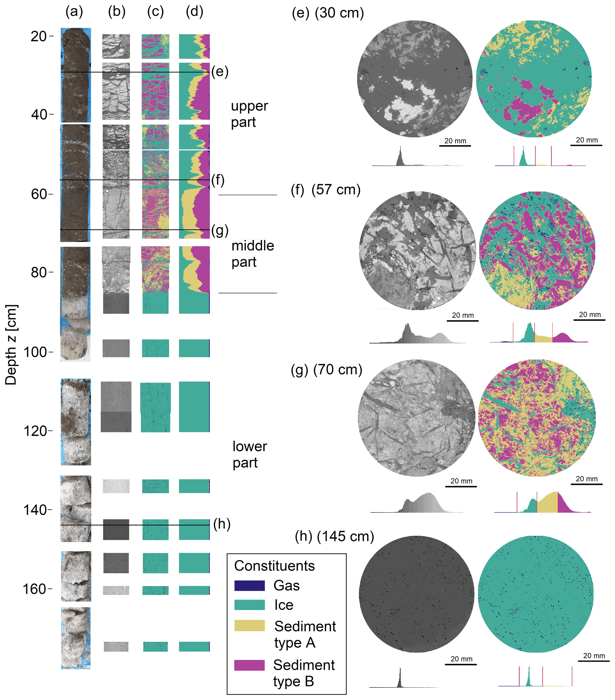
Figure 1 Overview of the studied permafrost core (a–d). Photography taken after drilling (a); absorption images from CT scanner after preprocessing (b) and after segmentation (c); volumetric contents of gas, excess ice, and sediment types A and B (d). The right part (e–h) shows exemplary horizontal slices of the preprocessed and segmented CT images, as well as the histograms of greyscale values, which are indicative of the constituents' densities.

2.4 Estimating the composition of the sediment types

Since the CT images do not allow the estimation of the composition of the sediment types directly, we used the volumetric total ice (θ_i), mineral (θ_m), and organic (θ_o) contents that were determined in the lab (Sect. 2.3) to infer their composition statistically. For this, we assumed them to be saturated and thus composed of organic matter (${\mathit{\gamma }}_{\text{A/B,o}}\in [\mathrm{0},\mathrm{1}]$), mineral grains (${\mathit{\gamma }}_{\text{A/B,m}}\in [\mathrm{0},\mathrm{1}]$), and pore ice (${\mathit{\gamma }}_{\text{A/B,pi}}\in [\mathrm{0},\mathrm{1}]$):

$$\begin{array}{}\text{(4)}& \begin{array}{rl}& {\mathit{\gamma }}_{\text{A,pi}}+{\mathit{\gamma }}_{\text{A,o}}+{\mathit{\gamma }}_{\text{A,m}}=\mathrm{1}\\ & {\mathit{\gamma }}_{\text{B,pi}}+{\mathit{\gamma }}_{\text{B,o}}+{\mathit{\gamma }}_{\text{B,m}}=\mathrm{1}.\end{array}\end{array}$$

Note that the pore ice fractions γ_A/B,pi correspond to the porosity of the respective sediment type under the assumption of saturated sediment. For each of the j=1…N_j samples the following linear equation system can be formulated:

$$\begin{array}{}\text{(5)}& \begin{array}{rl}{\mathit{\theta }}_{\text{o}}\left(z_j\right)& ={\mathit{\gamma }}_{\text{A,o}}{\mathit{\theta }}_{\text{A}}\left(z_j\right)+{\mathit{\gamma }}_{\text{B,o}}{\mathit{\theta }}_{\text{B}}\left(z_j\right)\\ {\mathit{\theta }}_{\text{m}}\left(z_j\right)& ={\mathit{\gamma }}_{\text{A,m}}{\mathit{\theta }}_{\text{A}}\left(z_j\right)+{\mathit{\gamma }}_{\text{B,m}}{\mathit{\theta }}_{\text{B}}\left(z_j\right)\\ {\mathit{\theta }}_{\mathrm{i}}\left(z_j\right)& =\underset{{\mathit{\theta }}_{\text{pi}}\left(z_j\right)}{\underbrace{(\mathrm{1}-{\mathit{\gamma }}_{\text{A,m}}-{\mathit{\gamma }}_{\text{A,o}}){\mathit{\theta }}_{\text{A}}\left(z_j\right)+(\mathrm{1}-{\mathit{\gamma }}_{\text{B,m}}-{\mathit{\gamma }}_{\text{B,o}}){\mathit{\theta }}_{\text{B}}\left(z_j\right)}}\\ & +{\mathit{\theta }}_{\text{ei}}\left(z_j\right),\end{array}\end{array}$$

where Eq. (4) was used to express the pore ice fraction of sediment types A and B in terms of their respective organic and mineral fractions. For this over-determined system of equations we performed a linear least-squares regression using the scikit-learn Python package (https://scikit-learn.org/stable/modules/generated/sklearn.linear_model.LinearRegression.html, last access: 29 August 2022) to find the best-fitting parameters ${\widehat{\mathit{\gamma }}}_{\text{A/B,m/o}}$. For the left-hand side of equation system (5) we took as input the laboratory estimates of the mineral, organic matter, and total ice contents (θ_m/o/i(z_j)). For the right-hand side we took as input the estimates of the volumetric fractions of the sediment types A and B and the excess ice from the CT analysis (θ_A/B/ei(z_j)), averaged over the same depth intervals as the laboratory samples.

Finally, we used the resulting best-fitting parameters (${\widehat{\mathit{\gamma }}}_{\text{A/B,m/o/pi}}$) and the high-resolution profiles from the CT analysis (θ_A/B/ei/a(z)) as input to the equations (5) to determine a high-resolution profile for the organic (θ_o(z)), mineral (θ_m(z)), and total ice contents (θ_i(z)) of the entire core. Note that we refer to the profiles θ_A/B/ei/a(z) as being directly derived from the CT images, while the profiles θ_o/m/i(z) were indirectly derived from the CT images as they require the composition of the sediment types to be estimated through the statistical regression against laboratory measurements.

Figure 2 Vertical profiles of volumetric gas (a), ice (b), organic (c), and mineral (d) contents of the core. Gas and excess ice were derived directly from the CT images, while pore ice, organic, and mineral contents were derived indirectly using estimates of the composition of the sediment types obtained from a linear regression against laboratory measurements. The lower panels (e, f, g) show the agreement between the CT-derived and the laboratory-measured contents. Note the different ranges of the horizontal axes for the different constituents. Evaluation metrics of the linear fit between CT-derived and lab-measured values are provided in Table 1.

3 Results

3.1 General composition and cryostructures

Figure 1 provides an overview of the entire core after drilling (a), CT scanning (b), and image segmentation (c, d). The photography of the core (Fig. 1a) allowed us to distinguish two major compartments: the first ranges from about 20 to 85 cm depth and contains sediment with ice inclusions; the second extends from about 85 cm depth to the end of the core and is essentially composed of massive ice originating from an ice wedge. Note that we subsequently use the term excess ice to refer to both segregation ice and massive wedge ice contained in the core.

The CT image of the core (Fig. 1b) allowed us to identify characteristic cryostructures such as layered (e.g. Fig. 1e) and reticulate (e.g. between 30 and 40 cm depth) in the upper part of the core. In the lower part, we identified small inclusions of gas (“bubbles”) of circular or vertically elongated shape within the massive ice (Fig. 1h).

The image segmented into gas, excess ice, and two sediment types (Fig. 1c) suggested a further subdivision of the sedimentary compartment into an excess ice-rich upper part from 20 to about 60 cm (e.g. Fig. 1f) and a sediment-rich part between 60 and 85 cm depth (e.g. Fig. 1g). Hence, we subsequently distinguish three major parts of the core: the core section between 20 and 60 cm depth as the “upper” part, the section between 60 and 85 cm as the “middle” part, and the section below 85 cm depth as the “lower” part (see Fig. 1).

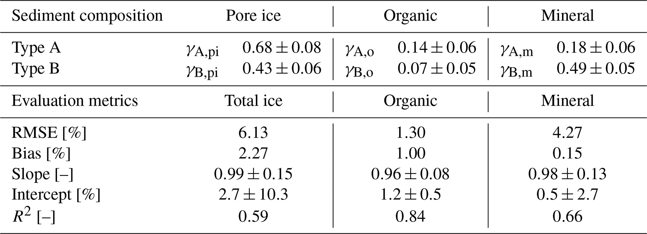
Table 1 Upper part: composition of the sediment types A and B derived through a linear regression against laboratory measurements (see Eqs. 4 and 5; given ranges are the standard errors of the regression). Lower part: evaluation metrics of the agreement between CT-derived and lab-measured volumetric organic, mineral, and total ice contents (cf. Fig. 2e–g; RMSE: root mean square error; bias: mean difference CT−lab; slope and intercept of a straight line fit (ranges are standard errors); R²: coefficient of determination).

3.2 Direct estimation of gas and excess ice contents

From the segmented CT images, we directly obtained vertical profiles of volumetric gas (θ_a(z); Fig. 2a) and excess ice (θ_ei(z); Fig. 2b) contents. As a general pattern, we found that gas contents are positively correlated with excess ice contents since gas contents well above 1 % were found in the upper (excess ice-rich) part of the core, in the lower (pure excess ice) part, and also at the positions of ice lenses throughout the sedimentary part of the core. In deviation from this pattern, gas contents were relatively low in the part around 30 cm depth despite the presence of ice lenses (Fig. 2a, b). We hypothesize that partial melting of the excess ice in the uppermost part, e.g. in particularly warm and wet thawing seasons, could have destroyed gas inclusions, causing the absence of significant amounts of gas just below the active layer. Vice versa, this suggests that the excess ice layers at depths below 35 cm preserved gas inclusions and could have been present since the ice formation. In the lower part of the core that consists of almost pure excess ice, gas contents were found to be almost constant at a level of about 2 % to 3 %, which is typical of wedge ice. As gas contents cannot be determined directly in the laboratory, we could not compare the CT-derived profile to independent estimates.

Excess ice contents were found to be >20 % in the upper part and even exceed 30 % in the section between 40 and 60 cm depth. Furthermore, the vertical profiles allowed us to identify several ice layers at approximate depths of 24, 30, 40, 48, 50, 57, 59, 70, and 78 cm, which are associated with distinct peaks in the profile where excess ice contents are exceeding 50 % to 60 %. In the lower part (>85 cm depth) the core is composed of >97 % of excess ice (massive wedge ice) with the remaining volume being filled with gas inclusions, as we found no significant sediment contents in the CT images. In the lower part as well as at the locations of thick ice lenses, the CT-derived excess ice contents agree well with the total ice contents determined from the lab samples (Fig. 2b), with typical deviations of about 10 % and maximum deviations of up to about 20 %, which can be explained by the relatively low pore ice content in these ice-rich sections. In sediment-rich sections of the core (e.g. between 60 and 70 cm depth), the total ice contents measured in the laboratory were substantially higher than the excess ice contents derived directly from the CT. This can be explained by the prevalence of pore ice contained in the sediment types A and B, which was included in the lab estimates, but could not be distinguished from the sediment matrix in the CT images.

3.3 Indirect estimation of pore ice, organic, and mineral contents

The vertical profiles of volumetric pore ice, organic, and mineral contents were calculated using Eq. (5) with the parameter values ${\widehat{\mathit{\gamma }}}_{\text{A/B,m/o/pi}}$ as determined by the linear regression (Table 1). The best-fitting parameters for sediment type A suggest an organic-rich soil (γ_A,o=0.14) with a high porosity (γ_A,pi=0.68). For sediment type B in turn, the composition parameters are indicative of a mineral soil (γ_B,m=0.49) with a lower porosity (γ_B,pi=0.43). We interpret sediment type A to correspond to organic matter inclusions within the sediment, while type B corresponds to a silty mineral matrix. We noticed that while the two sediment types occur more spatially separated in the upper part of the core (see Fig. 1e, f), they appear well mixed in the middle part, which is characterized by little excess ice (Fig. 1g). This difference could be linked to higher degrees of cryoturbation and other mixing processes which the organic-rich soil in the middle part of the core has undergone in the past.

The resulting vertical profile of the total ice content (${\mathit{\theta }}_{\mathrm{i}}\left(z\right)={\mathit{\theta }}_{\text{ei}}\left(z\right)+{\mathit{\theta }}_{\text{pi}}\left(z\right)$; dark line in Fig. 2b) shows a much-improved agreement with the ice contents determined from the lab samples (R²=0.59), compared to the directly determined excess ice profile (pale line in Fig. 2b). The largest deviations were found at the locations of ice lenses, suggesting that these are not resolved by the coarse sample resolution of about 2 to 3 cm. In the upper and middle parts of the core, the ice contents from the lab overall showed a low variability, ranging mostly between 60 % and 70 %. In contrast, the CT-derived total ice content profile resolved details much better and, for example, allowed the identification of the position of thick ice lenses. In addition, the CT-derived profiles allowed a robust distinction between pore and excess, ice which is not possible with the standard laboratory procedure.

We found similarly good agreement between the CT-derived profiles and the laboratory-measured volumetric organic matter (R²=0.84; Fig. 2c) and mineral (R²=0.65; Fig. 2d) contents (Table 1). Despite the fact that the laboratory measurements were used to derive the mineral and organic contents from the CT images, the good agreement provides credibility to the resulting high-resolution profiles, which provide a much more detailed picture of the composition of the core. We note that while the correspondence between CT profile and laboratory data is particularly good in the upper part of the core (<60 cm), the relative deviations were slightly higher in the middle part. An additional, separate regression as described in Sect. 2.4 but restricted to the data available for the middle part of the core could further improve the agreement between CT-derived and lab values. However, such an approach would violate the assumption that the two sediment types identified from the CT images are the same for the entire core.

4 Discussion and outlook

We successfully applied high-resolution CT as a non-destructive method to obtain the composition of a permafrost core. Compared to previous studies (Calmels and Allard, 2004), we report the highest spatial resolution in three dimensions of a permafrost core of Δx=50 µm. From the CT images we identified four different material classes: gas, excess ice, and two mixed sediment phases. Gas and excess ice were clearly distinguishable, confirming results of previous studies (Calmels and Allard, 2004, 2008; Calmels et al., 2012). Despite the high spatial resolution of the CT images, a robust distinction of the pore space filled with pore ice and the sediment matrix of the two mixed phases was not possible. The detection limit, which is about 2–3 times the voxel size, provides a technical constraint for the identification of pores (Vogel et al., 2010; Withers et al., 2021). Therefore, in this study only gas inclusions, cracks, and particles >100 µm were determined. With the employed CT scanner, a higher level of detail could have only been achieved by smaller fields of view and therefore at the expense of representativeness. Another issue is the image noise. Higher acquisition times could in theory improve the image quality but are problematic for frozen samples, as they could imply partial melting of the sample, which could in turn cause changes in the material properties or movement of the sample during image acquisition. Hence, the composition of the two sediment types could only be determined through an additional statistical regression against measurements obtained through destructive laboratory analysis of the core. The statistical regression revealed that the two sediment types have distinct compositions in terms of their volumetric pore ice, organic, and mineral contents, as well as different porosities, suggesting one type (A) to correspond to organic material and the other to be the (silty) mineral matrix (see Table 1). Overall, ground ice is the dominating constituent of the studied permafrost core, and it appears in different forms: excess ice in the form of ice lenses and massive wedge ice with minor gas inclusions and pore ice with volumetric fractions of about 43 % and 68 % in mineral and organic sediment types, respectively. In agreement with previous studies (Calmels and Allard, 2004), volumetric gas contents were small, with typical values of about 2 % and maximum values of up to 8 %. Volumetric organic matter contents ranged between 2 % and 10 % in the sedimentary part of the core and showed a tendency to increase with depth.

Though manual thresholding resulted in robust segmentation results which were validated against visual inspection and independent laboratory results, it is prone to some degree of subjectivity. Selecting the most applicable threshold is difficult because the resolution of the CT is often insufficient to resolve the phase or object of interest completely. For example, the pore ice inclusions within the mineral matrix are often smaller than the spatial resolution of the CT. The resulting grey value of a voxel is then a mixture of low-density ice and high-density minerals and may straddle around the threshold depending on the exact proportions within such a partial volume voxel. In the future, the segmentation could be simplified by choosing a more appropriate greyscale normalization than the percentile method. For example, homogeneous reference materials could be used to standardize the grey values prior to segmentation similar to Hounsfield units so that the same set of thresholds could be applied to all CT images (Koestel, 2018). For permafrost soils, the histogram peaks of gas and ice could be used. If these are not abundant enough to evoke distinct peaks, then rods of different material density (e.g. plastic and aluminium) could be attached along the entire ice core so that they are present in all image segments to be identified as reference materials. Segmentation of such normalized CT images by unsupervised classification (e.g. k-means clustering) can be hampered by the fact that the number of material classes differs among individual scans (Schlüter et al., 2014). Therefore, supervised, machine-learning-based image segmentation is recommended in which a classifier is trained by drawing a few test lines for each material class in small, but representative sub-volumes and then applied to all CT scans at once. State-of-the-art machine-learning toolkits allow the use of high-level image features like gradient and texture at several length scales in addition to normal greyscale information (Berg et al., 2019). In this way, material classes with overlapping greyscale ranges could be separated more accurately.

Our results introduce new perspectives on physical properties of permafrost and the processes shaping its microstructure. For example, the full potential of 3D microstructure analysis is harnessed when morphological properties of individual material classes are analysed since structure and geometry control soil processes and properties. This could include, for example, the aperture and spatial density of ice inclusions in the sediment layer; the size, shape, and density of gas entrapment in the excess ice layers; and identification of organic and mineral clusters. Using this information would allow improved estimates of physical properties like the thermal conductivity or biochemical transport coefficients, which depend on the constituents as well as their spatial arrangement. Through additional analysis and combination with other measurements (e.g. age of material, grain size distribution) physical processes such as sediment and ice accumulation rate, cryoturbation, bubble microstructure (Opel et al., 2018), and pore resolution processes (Rooney et al., 2022) could be further studied with CT in the future. In summary, our work is an important step towards establishing microstructure CT imaging as a technique for (i) estimating the physical properties of permafrost ground and (ii) studying periglacial processes, allowing insights going far beyond classical destructive laboratory analyses.