the Creative Commons Attribution 4.0 License.
the Creative Commons Attribution 4.0 License.
 | 25 Aug 2022
Snow properties at the forest–tundra ecotone: predominance of water vapor fluxes even in deep, moderately cold snowpacks
Florent Domine
Daniel F. Nadeau
Matthieu Lafaysse
Marie Dumont
The forest–tundra ecotone is a large circumpolar transition zone between the Arctic tundra and the boreal forest, where snow properties are spatially variable due to changing vegetation. The extent of this biome through all circumpolar regions influences the climate. In the forest–tundra ecotone near Umiujaq in northeastern Canada ( N, W), we contrast the snow properties between two sites, TUNDRA (located in a low-shrub tundra) and FOREST (located in a boreal forest), situated less than 1 km apart. Furthermore, we evaluate the capability of the snow model Crocus, initially developed for alpine snow, to simulate the snow in this subarctic setting. Snow height and density differed considerably between the two sites. At FOREST, snow was about twice as deep as at TUNDRA. The density of snow at FOREST decreased slightly from the ground to the snow surface in a pattern that is somewhat similar to alpine snow. The opposite was observed at TUNDRA, where the pattern of snow density was typical of the Arctic. We demonstrate that upward water vapor transport is the dominant mechanism that shapes the density profile at TUNDRA, while a contribution of compaction due to overburden becomes visible at FOREST. Crocus was not able to reproduce the density profiles at either site using its standard configuration. We therefore implemented some modifications for the density of fresh snow, the effect of vegetation on compaction, and the lateral transport of snow by wind. These adjustments partly compensate for the lack of water vapor transport in the model but may not be applicable at other sites. Furthermore, the challenges using Crocus suggest that the general lack of water vapor transport in the snow routines used in climate models leads to an inadequate representation of the density profiles of even deep and moderately cold snowpacks, with possible major impacts on meteorological forecasts and climate projections.
- Article
(6037 KB) - Full-text XML
-
Supplement
(462 KB) - BibTeX
- EndNote


Seasonal snowpacks significantly increase surface albedo (Cohen and Rind, 1991) and soil insulation (Meredith et al., 2019) and are thus critical to the planet's surface energy budget. In terms of spatial coverage, most seasonal snowpacks are found in the Arctic tundra and boreal forest biomes, with clear structural differences between the two. In the tundra, snow is usually shallow and has few distinct layers, whereas in the boreal forest, snow is deeper and has a more complex stratigraphy (Royer et al., 2021a). The transition zone between both biomes is called the forest–tundra ecotone and includes areas of short tundra vegetation alongside forest patches. As snow height depends on the density and height of the vegetation, the resulting snow cover is heterogeneous (Roy-Léveillée et al., 2014). Little is known about the snow structure in the forest–tundra ecotone, whose properties are evolving quite rapidly. Indeed, in their study, Ju and Masek (2016) found that 29.4 % of the land cover in Alaska and Canada showed greening trends. According to their findings, the greening occurred primarily in the tundra, with Quebec and Labrador being the most affected regions. Considering these significant changes, the extent of the forest–tundra ecotone throughout circumpolar regions, and its role in the global climate, more research is essential.
The weather conditions to which Arctic snow is typically exposed differ considerably from conditions generally found in the boreal forest further south (Sturm et al., 1995; Royer et al., 2021a). During the cold season in the Arctic tundra, very low air temperatures occur, together with low precipitation and high wind speeds. The result is a shallow snowpack with strong vertical temperature gradients, particularly in the fall when the ground is not yet frozen. Consequently, the dominant processes that shape the snowpack structure are the upward transport of water vapor, driven by the high temperature gradient, and the wind-induced compaction of the upper layers. This creates a low-density layer of depth hoar at the bottom and a hard, dense, wind-packed layer at the top (Domine et al., 2015, 2016b). Contrarily, in the boreal forest, air temperatures and precipitation are typically higher, while wind speeds are lower. Thus, the snowpack is deeper and the vertical temperature gradient is smaller (Royer et al., 2021a). This is particularly true for the boreal forest of northeastern Canada, where precipitation is relatively high compared to Alaska or Siberia (Groisman and Easterling, 1994). In forested environments, the compaction of the lower snow layers due to the weight of the upper layers becomes the dominant process, similar to alpine snow. This results in a snow cover that is spatially complex, where patches of typical Arctic snow blend into patches of alpine-like snow (Morin et al., 2013).
Detailed snow models like Crocus (Vionnet et al., 2012) and SNOWPACK (Bartelt and Lehning, 2002; Lehning et al., 2002a, b) have been applied in the Arctic with limited success. Studies using both Crocus (Barrere et al., 2017, and Royer et al., 2021b) and SNOWPACK (Gouttevin et al., 2018) show that Arctic snow is generally not well-modeled as the simulated density profiles do not match the observations. The lack of consideration of water vapor fluxes is suspected to be one of the main reasons for this (Domine et al., 2019). These models have been developed for alpine applications (Brun et al., 1989; Bartelt and Lehning, 2002), so the dominant process that controls the density profile in the models is the compaction that results from overburden. To overcome the lack of water vapor transport, Barrere et al. (2017), Gouttevin et al. (2018), and Royer et al. (2021b) all introduced modifications, without explicitly simulating water vapor transport, by increasing the maximum density of wind-induced snow compaction and adapting compaction to vegetation characteristics. This considerably improved the simulated density profiles and made them more comparable to observations at the site scale. On the other hand, simulations in the boreal forest have so far focused on the snow water equivalent (SWE). Studies in Canada (Bartlett et al., 2006; Oreiller et al., 2014) and Eurasia (Brun et al., 2013; Decharme et al., 2016) showed that the bulk density and the SWE could be simulated reasonably well within the boreal forest. However, the ability of those models to adequately simulate density profiles has yet to be tested.
Here, we present data on the internal physical properties of subarctic snowpacks to show that the transport of water vapor is an important process shaping the vertical snow density profile in both tundra and forest-dominated areas. Furthermore, we test the performance of the snow model Crocus and explore adjustments that compensate for the lack of a water vapor transport mechanism in the model.
2.1 Study site
Our study site was located in the Tasiapik valley, near the village of Umiujaq, Quebec, Canada ( N, W), on the eastern shore of Hudson Bay. The valley is 4.5 km long and 1.3 km wide, with elevations ranging from 0 to over 350 m above sea level, and is at the transition between the boreal forest and the Arctic tundra (Fig. 1). While the upper part of the valley is dominated by lichen and shrub tundra, the vegetation in the lower part consists of a mixture of forest and high shrubs. The shrubs (mainly dwarf birch Betula glandulosa) are between 0.2 and 1 m tall and cover 70 % to 80 % of the upper valley. The trees in the lower valley consist of black spruce (Picea mariana) up to 5 m tall and are estimated to cover roughly 20 % of the surface, while the majority is covered by medium-height shrubs (Salix spp. and Betula glandulosa) with willows reaching 2–3 m in height. Soils are predominantly sandy (Lemieux et al., 2020). While the soil in the upper part of the valley consists almost exclusively of sand (>90 %), the sand fraction is lower in forested areas, although no detailed measurements were available to quantify it. For more details about the study site, see Lackner et al. (2021) and Gagnon et al. (2019).
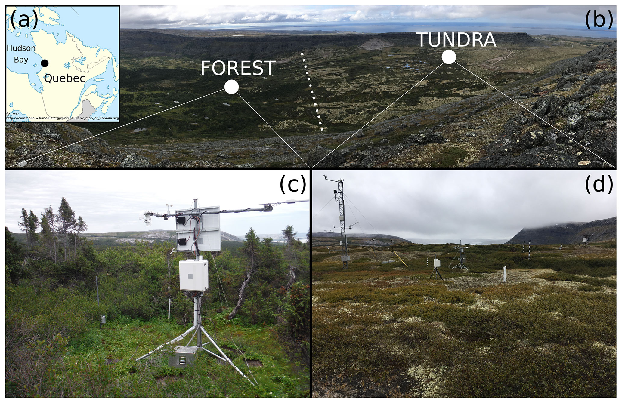
Figure 1(a) Location of the study site on the eastern shore of Hudson Bay, Quebec, Canada. (b) View of the Tasiapik valley towards the southwest, where the bottom (left) is covered with trees and the top (right) with tundra. Note the presence of the cuesta that delimits the valley. (c) FOREST station. (d) TUNDRA station. The dotted line is the boundary between the forested area and the shrub and lichen tundra.
2.2 Instrumental setup
Two stations were deployed in the valley. One was located in the middle part (FOREST, ≈80 m above sea level, see Fig. 1c) and the other was in the upper part (TUNDRA, ≈140 m above sea level, see Fig. 1d), with a distance of about 900 m between the two. The full radiation budget (CNR4, Kipp and Zonen, the Netherlands), air temperature and relative humidity (model HMP45, Vaisala, Finland), wind speed (A100, Vector Instruments, UK), and snow height (SR50, Campbell Scientific, USA) were measured at 2.3 m above ground at both sites. Additional measurements of wind speed and direction at a height of 10 m (model 05103, R. M. Young, USA), specific humidity (IRGASON, Campbell Scientific, USA), and precipitation at a height of 1.5 m (T200B, Geonor, USA) were also collected at TUNDRA, some 20 m away. The nearby trees did not obstruct the instruments at the FOREST site, and the surface underneath them was covered with grass. Snow temperature and thermal conductivity were measured at both sites using vertical poles equipped with TP02/TP08 heated needle probes (Hukseflux, the Netherlands). At TUNDRA, five needles were installed at heights of 4, 14, 29, 44, and 64 cm above the surface of a 10 cm thick lichen cover, whereas four needles were installed at FOREST in a patch of grass at heights of 4, 14, 29, and 64 cm above the base of the grass. The measurement principle of the TP02/TP08 heated needles is detailed in Morin et al. (2010) and Domine et al. (2015, 2016b). In short, each needle has a heated section and an unheated reference thermometer. The temperature of both is recorded when the needle is heated. The temperature difference between the two parts is then plotted against the logarithm of the time elapsed since the onset of heating. The effective snow thermal conductivity keff is inversely proportional to the slope of the resulting regression line. According to Domine et al. (2016b), the uncertainty in the thermal conductivity can be as high as 29 %. Lastly, three time-lapse cameras were installed at TUNDRA, which were used to qualitatively observe the transport of snow and to check to which extent the snow poles were covered.
Snow field surveys were conducted once or twice a year from 2012 to 2019 at different times throughout the winter (from January to April). During each field survey, snow pits were dug at several locations around the two study sites and further away in a perimeter of several hundred meters encompassing the site, with similar vegetation. A subset of the snow pit data (from 2012 to 2015) is presented in Domine et al. (2015). For each snow pit, the grain types of the layers were identified, and the density and temperature profiles were measured. For some snow pits, the thermal conductivity profiles were also measured with a portable instrument equipped with a TP02 heated needle. A 100 cm3 box cutter (Conger and McClung, 2009) and a field scale were used to measure the density profiles. The vertical spacing was mostly 3 cm between measurements but was increased to 5 cm for some snow pits, essentially those with deeper snow. At FOREST, snow pits were dug at some distance from trees, so snow interception can be neglected.
2.3 ISBA–Crocus land surface and snow models
Crocus and ISBA (interaction sol–biosphère–atmosphère: interactions between soil–biosphere–atmosphere) are part of the SURFEX modeling platform version 8.1 (http://www.umr-cnrm.fr/surfex/, last access: 20 January 2022) developed by Météo-France. ISBA (Noilhan and Planton, 1989; Decharme et al., 2011) simulates water and energy exchanges between the atmosphere, the vegetation, and the soil. In the presence of snow, Crocus is activated. Crocus (Vionnet et al., 2012) is a physically based snow scheme that can distinguish up to 50 snow layers each defined by their thickness, temperature, density, liquid water content, age, and microstructural properties (optical diameter and sphericity). These properties evolve according to physical processes such as thermal conduction, snow metamorphism, and snow compaction. When new snow is added to the snowpack following precipitation events, its temperature is equal to the temperature of the uppermost snow layer. In Crocus, there is no consideration for snow–vegetation interactions.
A first adaption of Crocus to Arctic snow has already been introduced in Vionnet et al. (2012) in order to simulate blowing snow events. However, the 1D nature of the model does not allow a direct simulation of snow erosion and accumulation and the associated effects (additional compaction and increased sublimation rates). Thus, two separate processes have been implemented in Crocus to simulate blowing snow: first, sublimation can be increased to simulate the loss of snow, effectively reducing the mass of the snowpack, or second, the upper layers can be densified without changing the mass of the snowpack. For the first option, the quantity of sublimating snow is increased due to blowing snow episodes and follows the parametrization of Gordon et al. (2006), with the corresponding mass being subtracted from the snowpack. This option was not activated here in order not to artificially increase sublimation rates. In other words, sublimation is included in the study, but it is not increased by the blowing snow parameterization. For the second option, enabled here, the upper snow layers are additionally compacted according to the following equation:
where ρ is the current density of the upper snow layer, ρmax is the maximum density (set as 350 kg m−3 by default), and τ is a timescale set to 48 h. We raised the maximum value ρmax to 600 kg m−3, as suggested in Barrere et al. (2017) and Royer et al. (2021b) for Arctic applications.
Barrere et al. (2017) showed that the default version of Crocus was not capable of correctly simulating density profiles that were observed in Arctic snow. Preliminary simulations at our study site led to the same conclusion. We therefore deemed it relevant to explore modifications to the code that are all based on physical processes specific to the Arctic environment in order to remedy this shortcoming. We chose to focus on three key processes that were suggested by Barrere et al. (2017), Gouttevin et al. (2018), and Royer et al. (2021b): densification by wind, particularly the densification of fresh snow (Snowfall), compaction due to overburden (Compaction), and the lateral transport of snow during blowing snow events (Blowing snow). Note that our goal here is not to propose an optimal parametrization of these processes but rather to explore whether their adaptation to the low-Arctic context can improve simulations. For the first process Snowfall, there are three options for fresh snow density in the default version of Crocus (Vionnet et al., 2012, Schmucki et al., 2014 and Anderson, 1976), as detailed in Lafaysse et al. (2017). All three depend on wind speed and air temperature (except for the one from Anderson, 1976, which depends on temperature only). All three lead to rather low densities given the cold temperatures typically found in the Arctic. As in Royer et al. (2021b), we used the parametrization of Vionnet et al. (2012) for the fresh snow density ρn:
where aρ=109 kg m−3, bρ=6 , and cρ = 26 are parameters, and Tfus is the melting point of water. Equation (2) is driven by air temperature (Ta) and wind speed (U). Motivated by the fact that the top layers of the snowpack are usually very hard in Arctic environments, we opted to increase the density of fresh snow by doubling the parameter aρ and multiplying cρ by 5. These values were obtained with a sensitivity analysis in which we varied aρ and cρ in order to obtain a good agreement between the simulated and observed densities of the top of the snow cover. Vegetation traps snow and prevents the subsequent transport of snow by wind (Essery and Pomeroy, 2004), thus reducing the effect of wind on the density of fresh snow. We therefore chose to apply this new parametrization only when the height of the snowpack exceeds the vegetation height. When that is not the case, the default parameters from Vionnet et al. (2012) are used. Note that this parametrization includes densification effects of the wind during periods when the snow crystals are still airborne (fragmentation during saltation), as well as when they are deposited onto the snowpack.
The process Compaction makes snow densification dependent on canopy height. This takes into account the stabilizing effect of vegetation on the snow cover and follows observations of Domine et al. (2016a) that density within shrubs is significantly lower than above. In Crocus, the snow layer thickness D is updated at each time step dt to account for compaction and the increase in snow density. Herein, we introduce a parameter c acting to reduce the effective overburden and as such the compaction.
where σ is the overburden stress, and η is the viscosity. This allows us to modulate the increase in density due to compaction from 0 % to 100 %, where 0 % means no increase in density and 100 % means that the default procedure is applied. In this study, we selected a fixed value of 0.05, meaning the increase was reduced to 5 % of its default value. This value was obtained by comparing observed and simulated density profiles and varying c until a good agreement with observations was obtained. This procedure was applied only for half the height of the canopy, following observations from Ménard et al. (2014) and Belke-Brea et al. (2020) highlighting the bending of shrubs under the weight of snow.
Lastly, a simple scheme to compensate for not considering any blowing snow process (Blowing snow) was implemented in Crocus. High winds are very frequent in the Arctic, particularly during snowfall events, and thus blowing snow is extremely important (Li and Pomeroy, 1997). Due to the 1D nature of the model, it is not possible to explicitly take this phenomenon into account. However, ignoring the effects of blowing snow would greatly alter the simulation results. For offline simulations (no coupling to an atmospheric model), as presented here, no implementation of snow erosion or accumulation is available in Crocus. However, as stated earlier, a blowing snow process is already included in Crocus, but there snow is removed by increasing sublimation. As such, we implemented a linear equation that can modulate actual precipitation during blowing snow events to account for lateral transport. We opted for a process that can add snow without changing the sublimation in order to avoid the artificial alteration of this flux, and the precipitation rate was changed based on wind speed:
In Eq. (4), Pnew (in mm s−1) is the new precipitation rate, Pold (in mm s−1) is the old rate, U is the wind speed in m s−1, and a and b are coefficients. We obtained a reasonable agreement between the simulations and observations of the vertical density profiles and snow heights with a=0.1 and b=0.3. To account for the fact that blowing snow does not occur at low wind speeds, this option was only activated for wind speeds larger than 3 m s−1. Additionally, for wind speeds exceeding 10 m s−1, the increase in precipitation was limited to 3.1 times the original precipitation rate. Areas with tall vegetation act as sinks for wind-blown snow (Myers-Smith and Hik, 2013). A preliminary series of tests revealed that it was desirable to use Eq. (4) for FOREST only in order to remain as close as possible to the observed snow heights and focus our analysis on the internal properties of the snow cover.
In summary, we explored various (non-optimized) modifications that target processes known to be poorly managed by Crocus in the Arctic. At TUNDRA, the Snowfall and Compaction modifications were enabled, while at FOREST, the Snowfall, Compaction, and Blowing snow modifications were all activated.
2.4 Forcing data and model setup
The meteorological forcing variables of ISBA–Crocus are typical of those of a land surface model: air temperature, specific humidity, wind speed, incoming shortwave and longwave radiation, atmospheric pressure, and (solid and liquid) precipitation rates. Hourly observations of these variables at each of the two sites have been collected since 2012, except for atmospheric pressure, which has been available since June 2017, and precipitation, which was available since May 2016. The closest grid point data of ERA5 (Hersbach et al., 2020) to the study site data were used for the pressure before 2017 and were adjusted by applying a simple regression obtained with data from after 2017 between the measured data and the ERA5 data (R2=0.99 after the adjustment). We corrected the observed precipitation data for undercatch using the transfer function of Kochendorfer et al. (2017). For the partitioning of total precipitation into liquid and solid precipitation, we used a fixed threshold of 0.5 ∘C. The suitability of the threshold was tested using air temperature and observations of the precipitation type from Environment and Climate Change Canada (https://climate.weather.gc.ca, last access: 15 December 2021) at the Umiujaq airport (≈3 km away from TUNDRA). Thresholds between 0.3 and 0.8 ∘C were also tested, with little impact on the amount of snow.
The modeled soil columns had a total thickness of 12 m and were divided into 20 layers of increasing depth. The heat flux at the lower boundary of the lowest layer was set to zero.
Following the soil water content analysis from Lackner et al. (2021), we also adjusted two soil hydraulic parameters: the saturated soil water content and the field capacity. The soil composition was set to 95 % sand and 5 % silt (Gagnon et al., 2019) for TUNDRA and to 80 % sand, 15 % silt, and 5 % clay for FOREST based on estimates from several soil pits dug around the station where higher fractions of fine particles were found compared to TUNDRA. At both sites, the vegetation consisted of shrubs of 0.4 and 1.3 m height at TUNDRA and FOREST, respectively. To ensure the equilibrium of soil moisture and temperature, we initialized the model with a spin-up of 5 years (2012–2017). Note that because observations of precipitation from before 2016 were not available, raw ERA5 data had to be used for the 2012–2016 period, and for this reason the evaluation period is from 2017 to 2020.
We used a different forcing data set for each station. However, as some of the required variables were not available at FOREST, we used the precipitation, pressure, and specific humidity from TUNDRA. Given the proximity of the two sites, the differences between these variables are presumed to be very small.
3.1 Observed meteorological conditions
Before analyzing the snow characteristics, we compared the meteorological conditions at both sites (Fig. 2). Additionally, in Table 1, the mean difference and the mean absolute difference are shown for winters 2017–2018, 2018–2019, and 2019–2020.
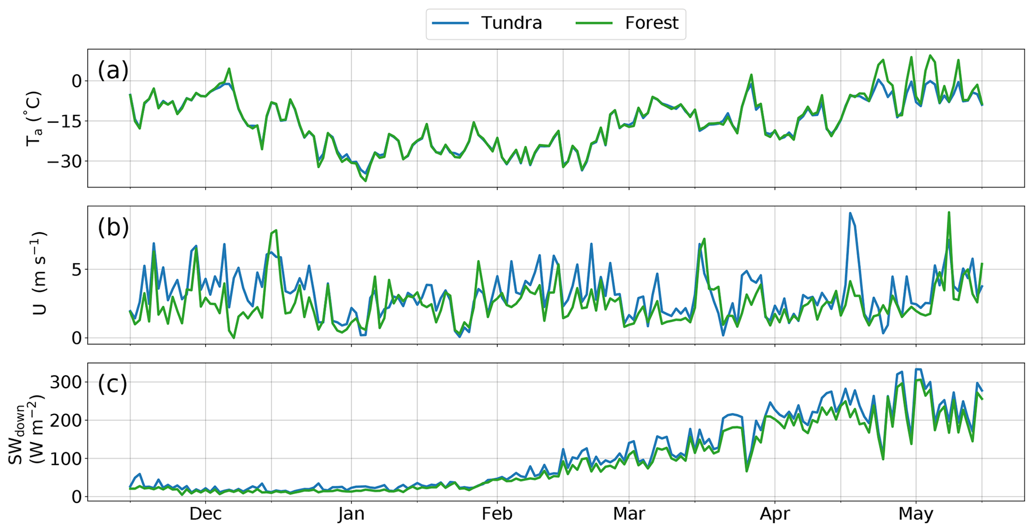
Figure 2Daily mean (a) air temperature Ta, (b) wind speed U, and (c) downwelling shortwave radiation SWdown measured at the two sites TUNDRA and FOREST for winter 2018–2019. Labeled tick marks on the x axis indicate the start of each month.
Table 1Mean difference (Δ) and mean absolute difference (MAD) between the TUNDRA and the FOREST sites of the air temperature Ta, wind speed U, and downwelling shortwave radiation SWdown for three winters 2017–2018, 2018–2019, and 2019–2020. Note that the radiation at TUNDRA was replaced with FOREST data for parts of winter 2019–2020 (15 December to 1 March) due to problems with the instrument at TUNDRA.
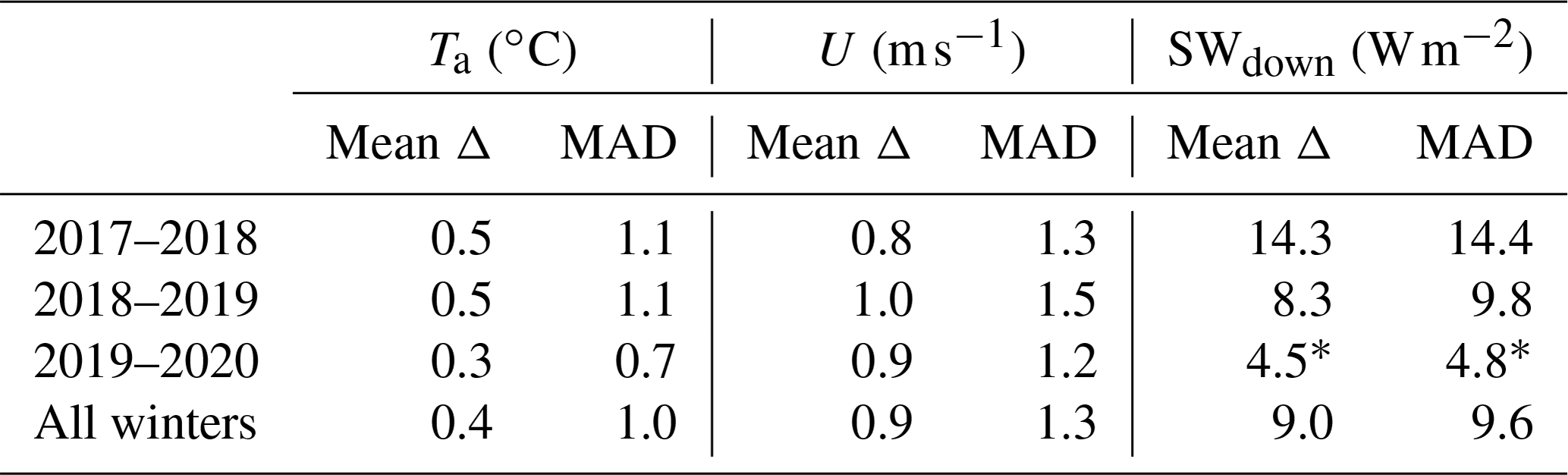
Air temperatures at the two stations were fairly similar. On average, TUNDRA was 0.4 ∘C colder than FOREST. Only occasional larger differences (≲2 ∘C) occurred until mid-April. After this point, air temperatures at TUNDRA were slightly colder than at FOREST. This trend was observed for all winters, with the exception of winter 2016–2017, when the difference was less pronounced. Wind speeds were consistently higher at TUNDRA, with a mean difference of about 0.9 m s−1 for all winters. Lastly, the disparity in downwelling shortwave radiation is also minimal, with a mean difference of 9.0 W m−2. The absolute difference in downwelling shortwave radiation between TUNDRA and FOREST increased in spring from February onward, while the relative difference compared to the magnitude of the fluxes remained comparable throughout winter. The difference likely arises due to the location of FOREST further down the valley, where topographic shading is more significant. Due to the low density of trees, no significant differences in longwave radiation were observed.
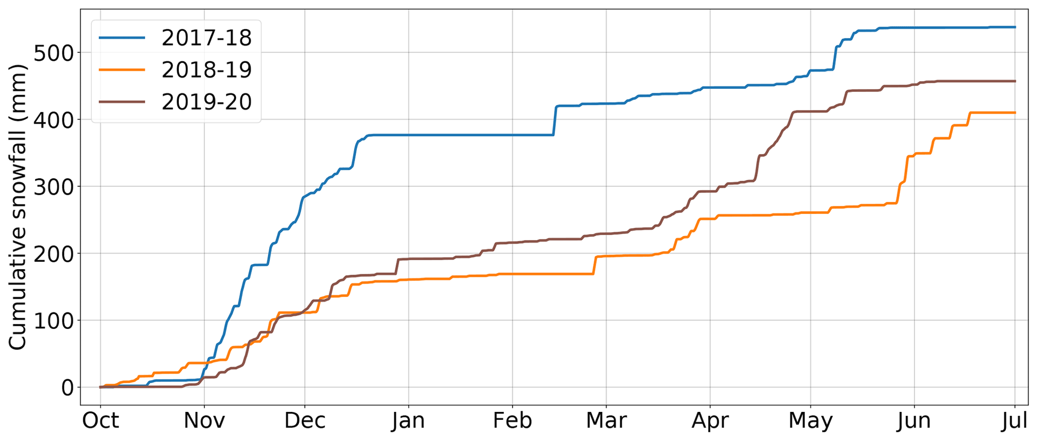
The cumulative solid precipitation for each of the three winters is shown in Fig. 3. Despite a pronounced interannual variability, the temporal patterns were very similar from one winter to the next. In fall, snowfall rates were quite sustained until mid-January, decreased temporarily, and then rose again in April.
3.2 Observations of snow properties
3.2.1 Snow height
Figure 4 shows the evolution of observed snow height for five consecutive winters (2015–2020) at TUNDRA and for three winters at FOREST. The onset of a seasonal snow cover consistently occurred in the second half of October each winter. Also, the snow cover formed at the same time at both sites. However, the subsequent evolution exhibited some differences between the two sites. At TUNDRA, a large fraction of the snow accumulation took place in the first few months of winter, up to mid-January. This was usually followed by a period of low precipitation (see Fig. 3) and thus low snow accumulation. Towards the end of winter, an increase in snowfall coincided with peak snow heights, typically in April or early May. At FOREST, the accumulation was more evenly distributed over the entire winter, and a gradual increase in snow height until April or early May was observed for all winters. The melt-out date at TUNDRA was strongly correlated with maximum snow height, and on average, this occurred in early June. However, depending on the maximum snow height, the melt-out date could occur half a month earlier or later, as was observed in winters 2016–2017 and 2019–2020. As the maximum snow height at FOREST was much more similar between the winters, the melt-out dates were also more consistent and took place around mid-June for all winters.
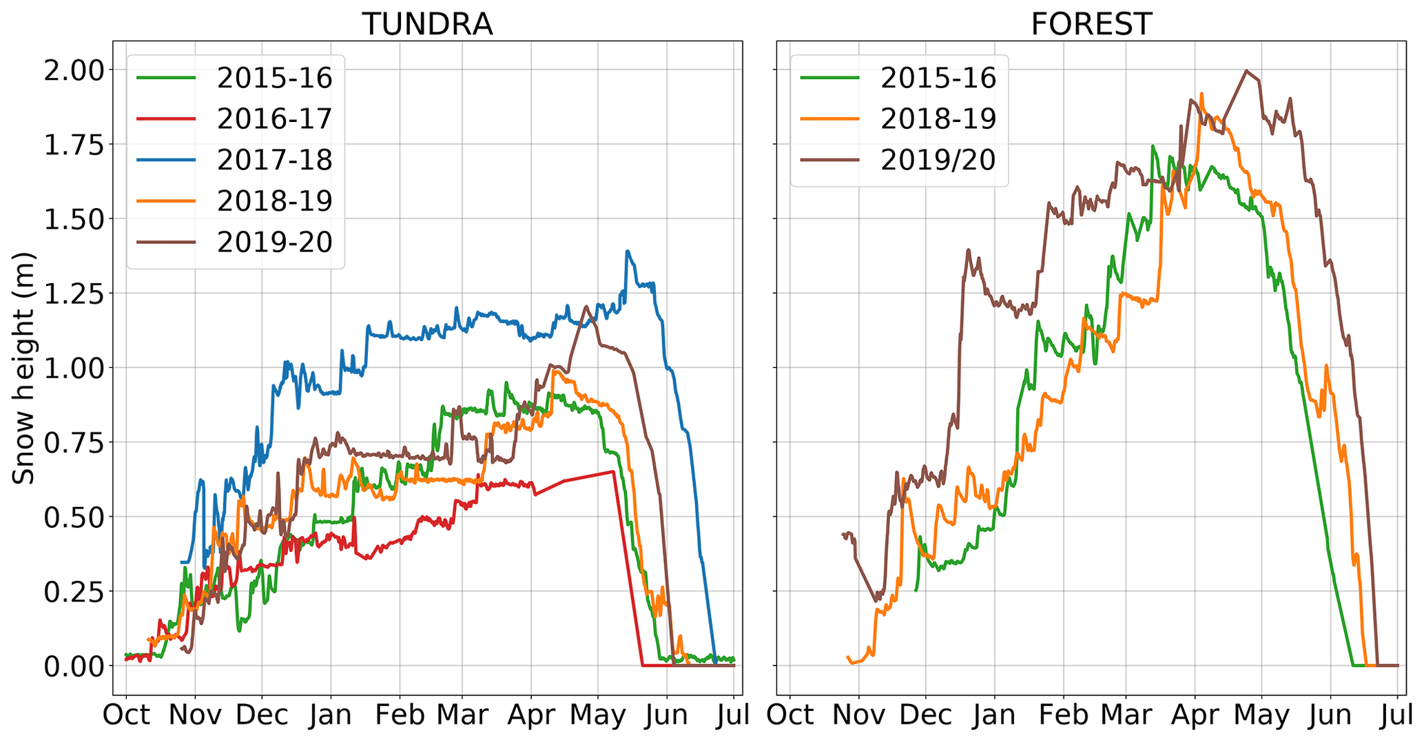
Figure 4Comparison of the measured snow height of TUNDRA and FOREST for several winters. When necessary, missing data were filled in with time-lapse camera observations of a graduated rod. Unfortunately, there was too much missing data from winters 2016–2017 and 2017–2018 at FOREST, so those winters are not presented here.
Although the observations presented in Fig. 4 are a good proxy for determining general snow heights at the sites, there is a high spatial variability. This variability is caused by the redistribution of snow by frequent high winds combined with differences in micro-topography and vegetation. For instance, on 12 April 2018, we made 172 measurements of the snow height within a 100 m radius of TUNDRA and observed heights varying between 50 and 210 cm, with a mean value of 109 cm. This is within 8 cm of the height measured by the automatic station that day (117 cm).
3.2.2 Stratigraphy
Differences in snow heights are reflected in the internal structure of the snowpack. Figure 5 shows simplified stratigraphies of representative snow pits from both TUNDRA and FOREST.
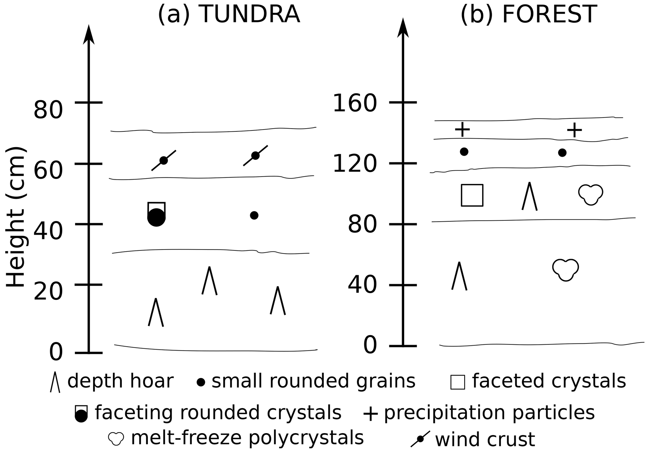
Figure 5Simplified stratigraphies from February 2014 representing typical snow conditions at sites (a) TUNDRA (25 February) and (b) FOREST (28 February). Note that the y scales are different for the two sites.
At TUNDRA, the depth hoar made up around half of the total depth. Just above the depth hoar, some layers of faceting or faceted rounded crystals were present, whereas the top of the snowpack usually consisted of a hard wind slab. The fraction of each layer type was highly variable. Furthermore, there were often more than three layers observed, and wind slabs alternating with layers of faceted crystals were fairly common.
The stratigraphy at FOREST was markedly different from that found at TUNDRA. While the depth hoar fraction was comparable to the one found at TUNDRA, melt–freeze forms were often present within these basal layers. On top of the depth hoar layers, there were often layers of small, rounded crystals. While the uppermost layers at TUNDRA were usually made up of a wind slab, fresh snow (precipitation particles) was often found in the top layer of the snowpack at FOREST, as seen in Fig. 5.
3.2.3 Density and thermal conductivity
On the left side of Fig. 6, the density profiles of 29 snow pits that were dug in the months of January, February, and March from the years 2012–2019 are shown, along with their means. They were all dug in the surrounding area of TUNDRA or environments with a similar canopy cover. The same is shown on the right side of Fig. 6 but for 16 snow pits that were dug near FOREST or in environments with a similar canopy cover. In order to make the profiles comparable, every measurement height was divided by the height of the respective snow cover.
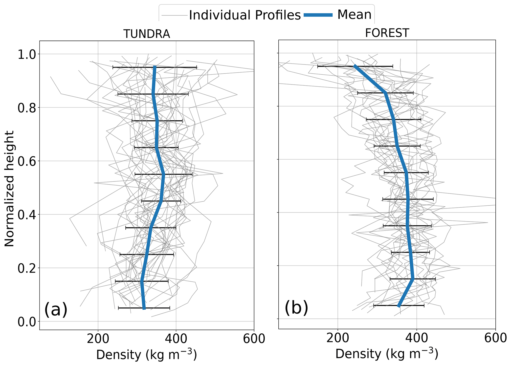
Figure 6Snow density profiles from 29 snow pits near TUNDRA and 18 snow pits near FOREST collected between January and March from the years 2012 to 2019. For better comparability, snow heights were normalized. The mean of all profiles is also shown, together with the standard deviation.
Due to the contrast in snow heights between the two sites, the vertical density profiles also showed significant differences. While mean snow density slightly increased with height at TUNDRA, there was a clear decrease in density for the upper 50 % and a very slight decrease between 15 % and 50 % of the snowpack at FOREST (only the lowermost snow part did not follow that decreasing trend). At TUNDRA, the mean density at the bottom of the snowpack was around 315 kg m−3 and then rose to 350 kg m−3 in the middle and upper parts of the snowpack. At FOREST, snow in the basal part had a mean density of around 375 kg m−3, which decreased to less than 250 kg m−3 at the top. The scatter in the measured profiles was comparable at both sites, with fluctuations of 100 kg m−3 around the mean.
The profiles of snow thermal conductivity in Fig. 7 follow the same trend as the snow density in Fig. 6, with keff increasing with height at TUNDRA and decreasing with height at FOREST. At TUNDRA, keff values increased from 0.1 in the depth hoar layers to slightly more than 0.2 in the wind slab. At FOREST, the thermal conductivity generally decreased from 0.2 in the basal part to almost 0.1 in the top layer. However, the lowermost snow layer at FOREST did exhibit very low thermal conductivity (≈0.1 ), indicating a departure from the general trend of the profile. The scatter of the measured thermal conductivity profiles is more pronounced at both sites when compared to that observed for density profiles, with a 178 % increase in the variance at TUNDRA and 214 % at FOREST. This scatter is particularly large in the layer with the highest thermal conductivity (e.g., the top layer at TUNDRA and the near-bottom layer at FOREST), with values ranging from 0.05 to over 0.4 .
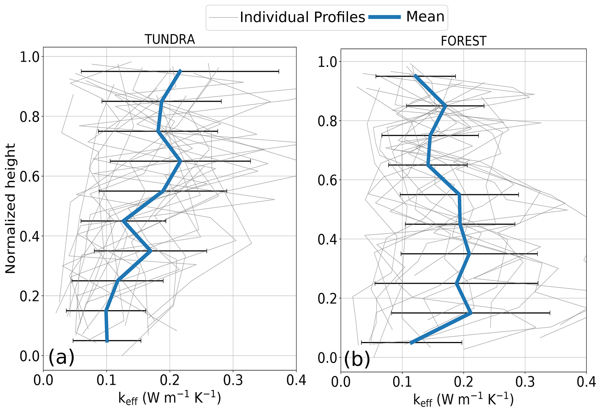
Figure 7Same as Fig. 6 but for snow thermal conductivity (keff). Note that only data from 21 snow pits for TUNDRA and 17 for FOREST were used as thermal conductivity measurements were not collected for every snow pit. The mean of all profiles is also shown, together with the standard deviation.
3.2.4 Soil and snow temperatures
Snow heights and thermal conductivity were quite different from one site to another, and consequently, the same variation can be assumed for snow and ground temperatures (Fig. 8).

Figure 8Snow (blue and red lines), ground (pink line), and air temperatures (grey line) at (a) TUNDRA and (b) FOREST for winter 2018–2019. Heights at which measurements were taken are relative to the ground surface. Air temperature Ta was measured at 2.3 m above ground. The values correspond to measurements collected once every other day at 05:00 EST.
As air temperatures and other meteorological forcings (Fig. 2) only slightly varied between the two sites, differences between snow and ground temperatures likely arose from discrepancies in the snowpack properties. The most noticeable divergence occurred near the soil–snow interface. At FOREST, the ground remained unfrozen until January and then dropped to its lowest value at slightly below −1 ∘C. The snow temperature at 14 cm very closely followed the ground temperature but was 1 ∘C colder. At TUNDRA, the ground at 9 cm depth froze as early as mid-November and then in March dropped to the lowest values of below −11 ∘C, about 10 ∘C colder than at FOREST. At TUNDRA, the snow temperature at 11 cm was on average 3 ∘C colder than the ground temperature. The temperatures higher up in the snowpack (53 cm for TUNDRA and 64 cm for FOREST) followed air temperature fluctuations more closely. At TUNDRA, the difference between air and the temperature at 64 cm varied between 0 and 5 ∘C. At FOREST, this difference reached up to 10 ∘C, with an evident decoupling between air and the temperatures at 64 cm beginning in early February.
3.3 Modeling
3.3.1 Snow height
In Fig. 9, the snow heights at TUNDRA and FOREST during winters 2018–2019 and 2019–2020 are compared to two different simulations, one using the default configuration of Crocus and one using the adjusted version of Crocus presented in Sect. 2.3.
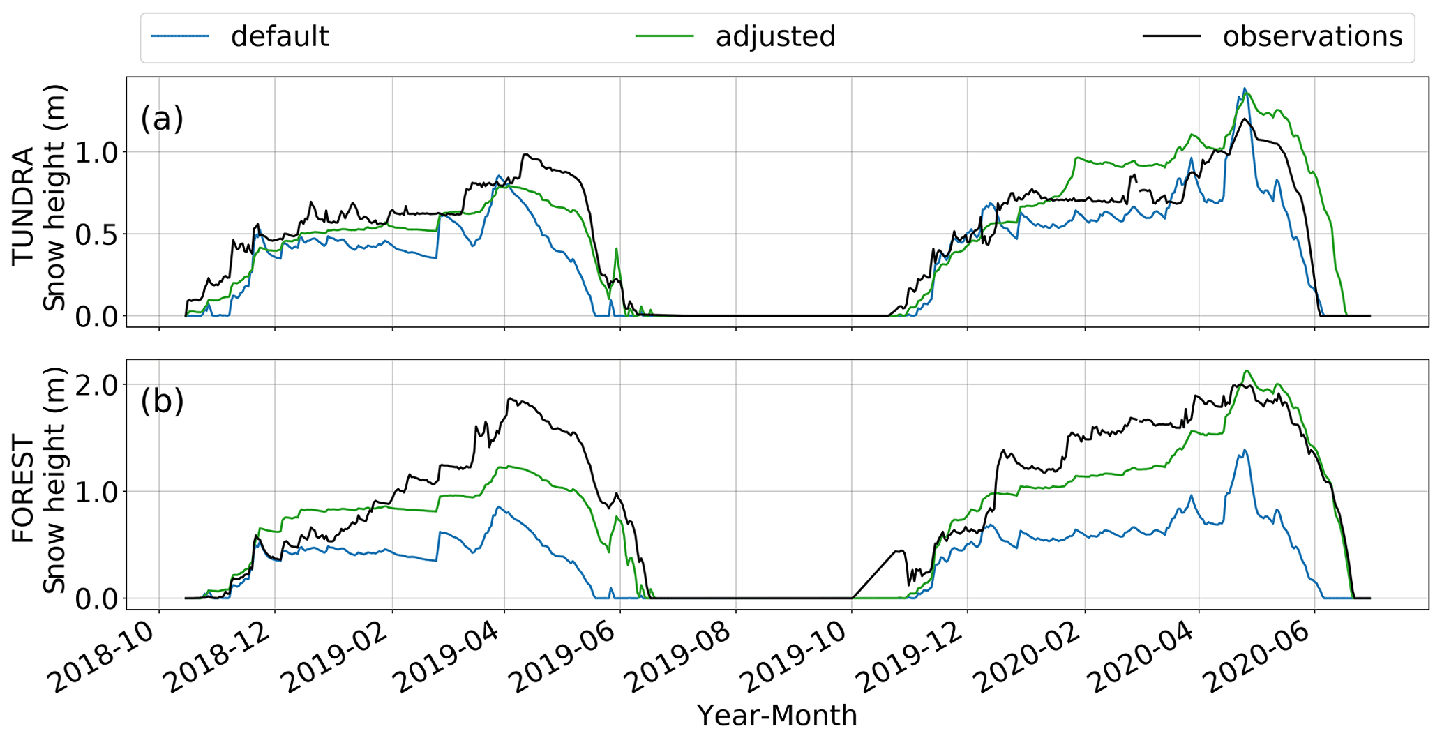
Figure 9Evolution of simulated and observed snow heights during winters 2018–2019 and 2019–2020 at (a) TUNDRA and (b) FOREST. Two different simulations are shown: the default version of Crocus and the adjusted version, in which modifications to the compaction and snowfall modules are activated at the two sites. At FOREST, a blowing snow module is implemented to account for snow transport by the wind.
At TUNDRA, the default version shows reasonable agreement with the observations. In winter 2018–2019, snow height is underestimated by 15 to 20 cm during the accumulation period, and the snow melt-out date is 12 d earlier than the observations. For winter 2019–2020, there is better agreement between the default version of Crocus and the observations, with a mean negative bias of 10 cm, leading to a modeled melt-out date that is just 2 d later than the observed date. Simulations with the adjusted version of Crocus (including the processes Compaction and Snowfall) for TUNDRA show an increased snow height of 10 to 20 cm compared to the default version. For winter 2019–2020, this leads to a delayed melt-out that is 15 d later than the observed date, while it is closer to observations in winter 2018–2019. One striking difference between the two versions is that the snow height fluctuations are dampened in the adjusted version of Crocus due to the reduced compaction and the heavier fresh snow.
Since the meteorological forcing is nearly the same at both sites, it is not surprising that the snow heights modeled by the default version of Crocus at FOREST are very similar to those at TUNDRA. As a result, the modeled snow heights of the default version are lower than the observed snow heights by a factor of 2. Thus, the simulated melt-out date is early by 1 month for winter 2018–2019 and by 16 d for winter 2019–2020. The adjusted version of Crocus (including the processes Compaction, Snowfall, and Blowing Snow) simulated snow heights that are much closer to those observed despite being underestimated by 10 to 70 cm. The melt-out date is better simulated, with a difference of 9 d in winter 2018–2019 and 0 d in 2019–2020.
One striking feature of both versions of the model is that simulated snow accumulation events do not always match with the observed accumulation events. This is most noticeable in February and March 2019. In February, all simulations show an accumulation, while no change in snow height was observed at TUNDRA. The opposite happened in March, when an increase in snow height was observed at the site, but no accumulation is reported in the simulation. This mismatch between observations and simulation is due to observed events of snow transport by wind, as confirmed by visually inspecting time-lapse photos.
Discrepancies in the simulation of snow height can also arise due to uncertainties of the SWE, i.e., the total snow mass per unit area. To verify whether this is the case, we compared simulations of the SWE with observations that were obtained using the density profiles (see Fig. S1 in the Supplement). At TUNDRA, there is a good agreement between the observed and simulated total snow mass. At FOREST, the model underestimates the SWE, similar to snow height in Fig. 9. Thus, the amount of blowing snow was higher than the one simulated by the model.
3.3.2 Density
The mean observed density profiles (Fig. 6) are compared to the default and adjusted model runs in Fig. 10. For calculating the mean of the simulated profiles, one profile per week during the months of January through March from 2017 to 2020 was taken and normalized, and then the average profile was calculated.

Figure 10Comparison between observed mean snow density profiles from Fig. 6 and the simulated density profiles from the default and adjusted versions of Crocus for (a) TUNDRA and (b) FOREST. The modeled mean profiles were obtained by averaging one snow profile per week between the months of January and March for both sites from 2017 to 2020.
Again, the default version of Crocus produces practically the same results at both sites, considering the small differences between the two forcing files. The mean from the default version shows a steep decline in density with height, as is typically observed for alpine snow. At the bottom of the snowpack, the density reaches almost 500 kg m−3, whereas the snow is very light at the top, with a minimum density of less than 90 kg m−3. At TUNDRA, the adjusted model fairly accurately simulated the density profile. It overestimates the density by ≈50 kg m−3 in the bottom 40 % of the snowpack, while it underestimates the density by 40 to 70 kg m−3 in the upper 60 %. However, whereas the mean absolute error of the default version is 127 kg m−3, it declines to 38 kg m−3 for the adjusted version. Moreover, the difference between the observations and the adjusted version is smaller than the variance of the observations.
At FOREST, the default version of Crocus performs better than at TUNDRA as observations showed a decrease in density with height. However, the density at the bottom of the snowpack is still largely overestimated (≈100 kg m−3) and even more underestimated at the top (≈160 kg m−3). Again, the adjusted version does reproduce the density profile significantly better than the default version. The mean absolute error decreases from 87 kg m−3 for the default version to 30 kg m−3 for the adjusted version. Similar to the profiles at TUNDRA, the variance of the observations is higher than the difference between the adjusted model and the observed profile.
4.1 Observations
We contrasted snow conditions at two sites located less than 1 km apart in the forest–tundra ecotone, each with very different vegetation characteristics (shrub tundra versus open forest). Meteorological conditions differed very slightly between the two sites (Fig. 2). At TUNDRA, air temperatures were a bit colder in spring for some of the winters we studied, and incoming shortwave radiation was slightly higher than at FOREST. The impact of air temperature differences on snow cover was modest as the largest deviations between the two sites were minor and confined to short periods. The difference in downwelling shortwave radiation can be explained by the location of FOREST further down the valley as for low solar angles in mid-winter, topographic shading is more pronounced there. Again, this does not heavily impact the snowpack as the albedo during this period is very high (≈0.85, see Lackner et al., 2022a). The high albedo means that most of the additional radiation at TUNDRA is reflected. The higher wind speeds at TUNDRA, however, have a considerable influence on the snowpack, leading to greater compaction and more fragmented crystals than at FOREST. The difference in wind speed between the two sites is most likely due to the lower surface roughness at TUNDRA, resulting from the shorter vegetation.
In addition to altered snow compaction at the surface, snow is also transported by the wind. During periods of high wind speeds (>3 m s−1), snow deposited on the surface is lifted up in the air and is typically transported several hundred meters away before settling back on the surface (Takeuchi, 1980). This phenomenon explains the large difference in snow height between the two sites, despite the likely similar amounts of total precipitation. As blowing snow events occur several times per week in the valley, snow is continuously transported from the upper parts of the valley (TUNDRA) to the lower part (FOREST). This leads to a gradual increase in snow height at FOREST. We see evidence that the taller vegetation at FOREST traps snow early in the season, while snow surveys that have been conducted at the very top of the valley (≈500 m north from TUNDRA) revealed a very shallow snowpack (≲40 cm). As snow erosion and deposition at TUNDRA likely balance each other, the snow height at TUNDRA is more closely correlated with the precipitation rate, which is typically low from January to March (see Fig. 3). As a result, the maximum snow height is on average twice as high at FOREST than at TUNDRA.
The differences in stratigraphy and density are a direct result of the different snow heights at the two sites. At FOREST, where there is more snow, the bottom fraction of the snowpack is more compacted by the weight of the overburden snow and is consequently denser. The deep snow cover insulates the soil more efficiently, maintaining warmer soil and creating a greater vertical gradient of snow temperatures throughout the winter (see Fig. 11). These conditions favor the kinetic growth of snow crystals and the development of thick depth hoar layers (Marbouty, 1980). At TUNDRA, where the snow height is considerably lower, the overburden and therefore the compaction of the lower layers are reduced, leading to basal sections of the snowpack of lower density. In part, due to the reduced snow height and fairly similar snow thermal conductivity, soil freezes earlier in the winter. Thus, the vertical gradient of snow temperature is greater at TUNDRA than at FOREST in early winter. However, the gradient decreases when soil freezes (Fig. 11), resulting in a comparable depth hoar fraction as at FOREST. At the top of the snowpack, wind speed shapes both the density and the stratigraphy. The lower wind speeds at FOREST lead to snow that is not as densely compacted in the top snow layers, which tends to preserve the shape of the snow crystals on the surface. This explains the observed lower density and higher abundance of precipitation particles. The opposite is true for TUNDRA, where wind speeds are higher, leading to denser top layers and precipitation particles that are rapidly fragmented and compacted into wind slabs. We hypothesize that the melt–freeze crystals are formed at both TUNDRA and FOREST due to short warm spells at the beginning of the winter. However, at TUNDRA, the high absolute values of the temperature gradient in December and January (see Fig. 11) trigger a more intense recrystallization compared to the FOREST site, and the melt–freeze crystals disappear at TUNDRA, while they remain at FOREST.
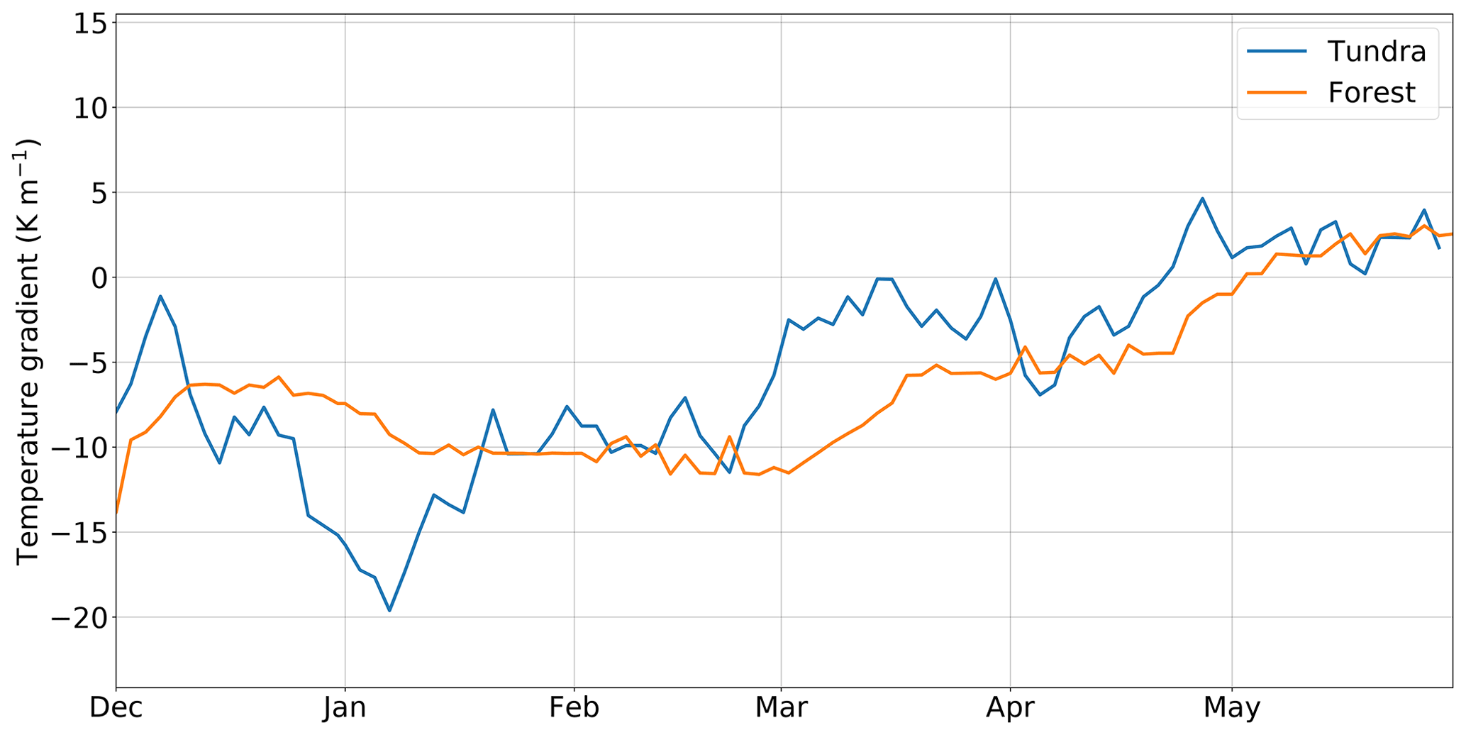
Figure 11Temperature gradient at the base of the snowpack for winter 2017–2018 at TUNDRA and FOREST. At TUNDRA, measurements were made at 11 and 21 cm, while the measurement heights were 4 and 14 cm at FOREST. Note that the measurement interval was 2 d; thus the peak gradients are likely to be larger than shown here. Negative gradients indicate higher temperatures close to the ground surface than those in higher snow layers.
A key factor that is often not included in relationships between snow density and thermal conductivity is the snow type (e.g., Sturm et al., 1997, Calonne et al., 2011, and Fourteau et al., 2021). Here, we hypothesize that this is the reason for the mismatch between the observed profiles of thermal conductivity in Fig. 7 and those of density in Fig. 6. Indeed, the detailed snow model SNOWPACK (Lehning et al., 2002b) improves the density–thermal conductivity relationship by also considering snow microstructure, i.e., snow type. The thermal conductivity profile at TUNDRA shows a very clear trend of increasing values with height, while there is only a very modest increase in density with height. One should note, however, that this could also be an artifact of the manual needle probe method as the soft snow at the bottom of the snowpack often breaks when the needles are inserted. Admittedly, the error of 29 % for the thermal conductivity measurements is rather high. However, in this study, the gradient of the profile is our main focus, reducing the impact of the uncertainty on a single measurement. Moreover, by taking the average of all samples the uncertainty is reduced according to or a factor of ≈4 with n=21 (TUNDRA) or n=15 (FOREST) samples.
4.2 Simulations
The accurate simulation of Arctic snow is complex as environmental factors are strikingly different compared to those in alpine environments, for which most of the sophisticated snow models have been developed (e.g., Brun et al., 1989, and Bartelt and Lehning, 2002). In recent studies, Arctic snow was simulated using Crocus and SNOWPACK snow models that included adaptations to account for higher wind compaction and the stabilizing effect of vegetation (Barrere et al., 2017; Gouttevin et al., 2018; Royer et al., 2021b). With these modifications, the simulations of the density profiles were significantly improved and thus more realistic. The changes proposed in those studies are similar to those we have implemented here, but some differences should be highlighted. Barrere et al. (2017) increased only the maximum density related to the parametrization of wind-induced snow compaction. Gouttevin et al. (2018) and Royer et al. (2021b) reduced the snow density in the vegetation layer, similar to what we have done in our study. However, we also tried to account for the bending of shrubs, and as such, snow compaction was reduced for only 50 % of canopy height and not the full height. The latter two studies also implemented different parametrizations for the density of fresh snow. While Gouttevin et al. (2018) based their parametrization on Antarctic data from Groot Zwaaftink et al. (2013), Royer et al. (2021b) used different parameters in the formulation of Vionnet et al. (2012) than those used here; namely they doubled the parameter cρ, while we quintupled it. Therefore, while there are clear similarities between the various approaches, the exact parametrizations used differ, which raises the question of the degree to which the parametrizations can be valid beyond their site of optimization.
The stabilizing influence of vegetation on the snow cover is not well documented. Ménard et al. (2014) observed and modeled the bending of shrubs, showing that they do not just remain at the same height when being buried in snow but rather bend to some extent. This suggests that the snow cover is not stabilized over the full height of the vegetation but rather on some fraction of it. Belke-Brea et al. (2020) investigated allometric equations for the exposed vegetation fraction of shrubs at the same site as in this study and explained deficiencies of the equation by a twofold structure of the shrubs, in which the lower part is more stable, while the upper part is more strongly bent. Thus, not taking the whole vegetation height as a zone where compaction is reduced seems a reasonable choice, particularly for higher shrubs as at FOREST.
Sustained high wind speeds are common in the Arctic and are thus an important factor influencing the snowpack. First, the top snow part is compacted by wind, and including this process into the model significantly improved the results. The second impact of strong winds is the transport of snow. This process is getting increased attention for snow simulations in mountainous environments (Marsh et al., 2020; Vionnet et al., 2021). We argue that it is equally important for applications in the Arctic environment. The simulated snow heights using the default version of Crocus differed from the observations by more than a factor of 2. Thus, future studies that use distributed snow models should take wind-driven snow transport into account. Combined with the impact of the snow height on the soil temperature (see Sect. 3.2.4), the importance of wind-driven snow transport is apparent and has a crucial impact on permafrost studies.
Finally, we would like to emphasize that we did not set out to find the best set of coefficients to simulate the two study sites. By including some key processes that are specific to the Arctic, our aim was to demonstrate that it is possible to simulate vertical density profiles reasonably well. The parameters in the processes Compaction and Snowfall were robust against small variations, meaning that the output of the model did not heavily depend on the exact choice of the parameters. However, as the model did not perform as well at TUNDRA as it did at FOREST, our results suggest that there is no single set of parameters that is best suited for both environments. The reason may be that these coefficient-fitting schemes are just compensating for the lack of description of upward water vapor fluxes in snowpacks, and the solution may be to actually include the latter in models. First attempts to do so have been made by Jafari et al. (2020) and Simson et al. (2021).
4.3 Water vapor fluxes
At TUNDRA, the snowpack showed a significant fraction of depth hoar, a snow type that solely originates under conditions with water vapor transport. Furthermore, the snow density increased towards the snow surface, whereas the opposite, a strongly decreasing pattern was simulated by Crocus, where compaction by overburden is the most important factor influencing the density. As our site receives a relatively large amount of precipitation, the findings show that water vapor transport is dominant over compaction even for deeper (up to 1 m) Arctic snowpacks. Hence, water vapor transport is the dominant process in shaping the density and thermal conductivity profile at our site, exceeding the importance of compaction due to overburden. Domine et al. (2016b) and Domine et al. (2019) have shown this for shallow high-Arctic snowpacks, but here, snow height is often more than 1 m and thus considerably deeper than in the high Arctic. Therefore, water vapor transport is prevalent for all Arctic regions, even for those with relatively large amounts of precipitation.
At FOREST, we found a depth hoar fraction similar to that at TUNDRA. While the density slightly decreases towards the surface, its gradient is still far inferior compared to simulations by Crocus. This leads to the conclusion that water vapor fluxes also play a significant role for deeper, moderately cold snowpacks present at FOREST.
Together with Sturm and Benson (1997), who demonstrated the importance of depth hoar for shallower (<1 m) snowpacks in forested subarctic regions, the results show that vapor fluxes have a critical impact on snowpack physics in the Arctic, the thin snowpack boreal forest, and the forest–tundra ecotone with deep snowpacks and therefore presumably in the boreal forest with deep snowpacks as well. Consequently, vapor fluxes cannot be neglected on the overwhelming majority of seasonal snowpacks.
We analyzed several winters of snow survey data at two sites that were located less than 1 km apart in the forest–tundra ecotone. One site was covered with sparse forest (FOREST), and one was an Arctic tundra (TUNDRA). We compared the snow properties of the two sites in terms of snow height, stratigraphy, density, thermal conductivity, and snow temperature. Additionally, we ran simulations with the snow model Crocus to explore model performance in both environments.
All the observed snow properties revealed marked differences between the two sites. Snow height was up to twice as high at FOREST than at TUNDRA due to wind-driven snow transport. This strongly affected the temperatures at the bottom of the snowpack as they were at times more than 10 ∘C colder at TUNDRA than at FOREST. A marked difference was also observed for the vertical density profiles. Snow density slightly increased with snow height at TUNDRA, indicating a profile that is typical of Arctic snow. In contrast, the density at FOREST decreased with height, which is more typical for alpine environments. In both cases, a substantial depth hoar layer occupied the lower portion of the snowpack.
The Crocus model failed to reproduce the density profile of both sites. Non-optimized adjustments to better represent typical Arctic processes (increased fresh snow density, reduced compaction within the canopy, and lateral transport of snow by the wind) have helped to improve the model outputs. However, simulations indicate a significant role of water vapor transport, showing that even deep, moderately cold snowpacks in the low-Arctic significantly differ from alpine-type snowpacks.
The significant amount of depth hoar and the Arctic-like density profile led to the conclusion that water vapor transport was the dominant metamorphic process at TUNDRA. At FOREST, the density gradient is towards slightly less dense layers at the top, indicating a role of overburden compaction more similar to alpine-like snow. Thus, after observing that water vapor transport is a crucial process in both deeper Arctic snowpacks and the deep, moderately cold snowpack in forested environments, we conclude that it is a critical process for the majority of seasonal snowpacks on Earth. Thus, the integration of water vapor fluxes in snow models, particularly in those coupled to climate models, is a pressing issue.
The source files of SURFEX code are provided at the Git repository (http://git.umr-cnrm.fr/git/Surfex_Git2.git, last access: 15 November 2021, Masson et al., 2013) with several code management tools (history management, bug fixes, documentation, interface for technical support, etc.). Registration is required; a description of the procedure is described at https://opensource.cnrm-game-meteo.fr/projects/snowtools/wiki/Procedure_for_new_users (last access: 15 January 2022).
Data will be available on the Pangaea repository (https://doi.pangaea.de/10.1594/PANGAEA.946538 (Lackner et al., 2022b).
The supplement related to this article is available online at: https://doi.org/10.5194/tc-16-3357-2022-supplement.
GL, DFN, and FD designed research. GL, DFN, and FD deployed and maintained instruments. GL and FD performed the field work. GL analyzed data with inputs from DFN and FD. GL set up the snow model Crocus with help from ML and MD. GL wrote the paper with inputs from DFN and FD and comments from MD and ML.
At least one of the (co-)authors is a member of the editorial board of The Cryosphere. The peer-review process was guided by an independent editor, and the authors also have no other competing interests to declare.
Publisher's note: Copernicus Publications remains neutral with regard to jurisdictional claims in published maps and institutional affiliations.
The authors are grateful to Denis Sarrazin for technical support of the CEN weather stations and the community of Umiujaq for permission to conduct our research.
This study was funded by Sentinel North, a Canada First Research Excellence Fund, under the theme 1 project titled “Complex systems: structure, function and interrelationships in the North”. This research has been supported by the Natural Sciences and Engineering Research Council of Canada (Discovery Grant), the French Polar Institute (IPEV) (grant no. 1042), and the Horizon 2020 program of the European 70 Commission (INTAROS; grant no. 727890). CNRM/CEN is part of Labex OSUG@2020 (ANR-10-LABX-0056).
This paper was edited by Masashi Niwano and reviewed by Charles Fierz and two anonymous referees.
Anderson, E. A.: A point energy and mass balance model of a snow cover, https://repository.library.noaa.gov/view/noaa/6392 (last access: 20 January 2022), 1976. a, b
Barrere, M., Domine, F., Decharme, B., Morin, S., Vionnet, V., and Lafaysse, M.: Evaluating the performance of coupled snow–soil models in SURFEXv8 to simulate the permafrost thermal regime at a high Arctic site, Geosci. Model Dev., 10, 3461–3479, https://doi.org/10.5194/gmd-10-3461-2017, 2017. a, b, c, d, e, f, g
Bartelt, P. and Lehning, M.: A physical SNOWPACK model for the Swiss avalanche warning: Part I: numerical model, Cold Reg. Sci. Technol., 35, 123–145, https://doi.org/10.1016/S0165-232X(02)00074-5, 2002. a, b, c
Bartlett, P. A., MacKay, M. D., and Verseghy, D. L.: Modified snow algorithms in the Canadian land surface scheme: Model runs and sensitivity analysis at three boreal forest stands, Atmos. Ocean, 44, 207–222, https://doi.org/10.3137/ao.440301, 2006. a
Belke-Brea, M., Domine, F., Boudreau, S., Picard, G., Barrere, M., Arnaud, L., and Paradis, M.: New allometric equations for Arctic shrubs and their application for calculating the albedo of surfaces with snow and protruding branches, J. Hydrometeorol., 21, 1–49, https://doi.org/10.1175/JHM-D-20-0012.1, 2020. a, b
Brun, E., Martin, E., Simon, V., Gendre, C., and Coleou, C.: An energy and mass model of snow cover suitable for operational avalanche forecasting, J. Glaciol., 35, 333–342, https://doi.org/10.3189/S0022143000009254, 1989. a, b
Brun, E., Vionnet, V., Boone, A., Decharme, B., Peings, Y., Valette, R., Karbou, F., and Morin, S.: Simulation of Northern Eurasian local snow depth, mass, and density using a detailed snowpack model and meteorological Reanalysis, J. Hydrometeorol., 14, 21955–21964, https://doi.org/10.1175/JHM-D-12-012.1, 2013. a
Calonne, N., Flin, F., Morin, S., Lesaffre, B., du Roscoat, S. R., and Geindreau, C.: Numerical and experimental investigations of the effective thermal conductivity of snow, Geophys. Res. Lett., 38, L23501, https://doi.org/10.1029/2011GL049234, 2011. a
Cohen, J. and Rind, D.: The Effect of Snow Cover on the Climate, J. Climate, 4, 689–706, https://doi.org/10.1175/1520-0442(1991)004<0689:TEOSCO>2.0.CO;2, 1991. a
Conger, S. and McClung, D.: Instruments and methods comparison of density cutters for snow profile observations, J. Glaciol., 55, 163–169, https://doi.org/10.3189/002214309788609038, 2009. a
Decharme, B., Boone, A., Delire, C., and Noilhan, J.: Local evaluation of the Interaction between Soil Biosphere Atmosphere soil multilayer diffusion scheme using four pedotransfer functions, J. Geophys. Res.-Atmos., 116, D20126, https://doi.org/10.1029/2011JD016002, 2011. a
Decharme, B., Brun, E., Boone, A., Delire, C., Le Moigne, P., and Morin, S.: Impacts of snow and organic soils parameterization on northern Eurasian soil temperature profiles simulated by the ISBA land surface model, The Cryosphere, 10, 853–877, https://doi.org/10.5194/tc-10-853-2016, 2016. a
Domine, F., Barrere, M., Sarrazin, D., Morin, S., and Arnaud, L.: Automatic monitoring of the effective thermal conductivity of snow in a low-Arctic shrub tundra, The Cryosphere, 9, 1265–1276, https://doi.org/10.5194/tc-9-1265-2015, 2015. a, b, c
Domine, F., Barrere, M., and Morin, S.: The growth of shrubs on high Arctic tundra at Bylot Island: impact on snow physical properties and permafrost thermal regime, Biogeosciences, 13, 6471–6486, https://doi.org/10.5194/bg-13-6471-2016, 2016a. a
Domine, F., Barrere, M., and Sarrazin, D.: Seasonal evolution of the effective thermal conductivity of the snow and the soil in high Arctic herb tundra at Bylot Island, Canada, The Cryosphere, 10, 2573–2588, https://doi.org/10.5194/tc-10-2573-2016, 2016b. a, b, c, d
Domine, F., Picard, G., Morin, S., Barrere, M., Madore, J.-B., and Langlois, A.: Major issues in simulating some arctic snowpack properties using current detailed snow physics models: Consequences for the thermal regime and water budget of permafrost, J. Adv. Model. Earth Sy., 11, 34–44, https://doi.org/10.1029/2018MS001445, 2019. a, b
Essery, R. and Pomeroy, J.: Vegetation and topographic control of wind-blown snow distributions in distributed and aggregated Simulations for an Arctic Tundra Basin, J. Hydrometeorol., 5, 735, https://doi.org/10.1175/1525-7541(2004)005<0735:VATCOW>2.0.CO;2, 2004. a
Fourteau, K., Domine, F., and Hagenmuller, P.: Impact of water vapor diffusion and latent heat on the effective thermal conductivity of snow, The Cryosphere, 15, 2739–2755, https://doi.org/10.5194/tc-15-2739-2021, 2021. a
Gagnon, M., Domine, F., and Boudreau, S.: The carbon sink due to shrub growth on Arctic tundra: a case study in a carbon-poor soil in eastern Canada, Environmental Research Communications, 1, 091001, https://doi.org/10.1088/2515-7620/ab3cdd, 2019. a, b
Gordon, M., Simon, K., and Taylor, P. A.: On snow depth predictions with the Canadian land surface scheme including a parametrization of blowing snow sublimation, Atmos. Ocean, 44, 239–255, https://doi.org/10.3137/ao.440303, 2006. a
Gouttevin, I., Langer, M., Löwe, H., Boike, J., Proksch, M., and Schneebeli, M.: Observation and modelling of snow at a polygonal tundra permafrost site: spatial variability and thermal implications, The Cryosphere, 12, 3693–3717, https://doi.org/10.5194/tc-12-3693-2018, 2018. a, b, c, d, e, f
Groisman, P. Y. and Easterling, D. R.: Variability and trends of total precipitation and snowfall over the United States and Canada, J. Climate, 7, 184–205, https://doi.org/10.1175/1520-0442(1994)007<0184:VATOTP>2.0.CO;2, 1994. a
Groot Zwaaftink, C. D., Cagnati, A., Crepaz, A., Fierz, C., Macelloni, G., Valt, M., and Lehning, M.: Event-driven deposition of snow on the Antarctic Plateau: analyzing field measurements with SNOWPACK, The Cryosphere, 7, 333–347, https://doi.org/10.5194/tc-7-333-2013, 2013. a
Hersbach, H., Bell, B., Berrisford, P., Hirahara, S., Horányi, A., Muñoz-Sabater, J., Nicolas, J., Peubey, C., Radu, R., Schepers, D., Simmons, A., Soci, C., Abdalla, S., Abellan, X., Balsamo, G., Bechtold, P., Biavati, G., Bidlot, J., Bonavita, M., De Chiara, G., Dahlgren, P., Dee, D., Diamantakis, M., Dragani, R., Flemming, J., Forbes, R., Fuentes, M., Geer, A., Haimberger, L., Healy, S., Hogan, R. J., Hólm, E., Janisková, M., Keeley, S., Laloyaux, P., Lopez, P., Lupu, C., Radnoti, G., de Rosnay, P., Rozum, I., Vamborg, F., Villaume, S., and Thépaut, J.-N.: The ERA5 global reanalysis, Q. J. Roy. Meteor. Soc., 146, 1999–2049, https://doi.org/10.1002/qj.3803, 2020. a
Jafari, M., Gouttevin, I., Couttet, M., Wever, N., Michel, A., Sharma, V., Rossmann, L., Maass, N., Nicolaus, M., and Lehning, M.: The impact of diffusive water vapor transport on snow profiles in deep and shallow snow covers and on sea ice, Front. Earth Sci., 8, 249, https://doi.org/10.3389/feart.2020.00249, 2020. a
Ju, J. and Masek, J. G.: The vegetation greenness trend in Canada and US Alaska from 1984–2012 Landsat data, Remote Sens. Environ., 176, 1–16, https://doi.org/10.1016/j.rse.2016.01.001, 2016. a
Kochendorfer, J., Nitu, R., Wolff, M., Mekis, E., Rasmussen, R., Baker, B., Earle, M. E., Reverdin, A., Wong, K., Smith, C. D., Yang, D., Roulet, Y.-A., Buisan, S., Laine, T., Lee, G., Aceituno, J. L. C., Alastrué, J., Isaksen, K., Meyers, T., Brækkan, R., Landolt, S., Jachcik, A., and Poikonen, A.: Analysis of single-Alter-shielded and unshielded measurements of mixed and solid precipitation from WMO-SPICE, Hydrol. Earth Syst. Sci., 21, 3525–3542, https://doi.org/10.5194/hess-21-3525-2017, 2017. a
Lackner, G., Nadeau, D. F., Domine, F., Parent, A.-C., Leonardini, G., Boone, A., Anctil, F., and Fortin, V.: The effect of soil on the summertime surface energy budget of a humid subarctic tundra in northern Quebec, Canada, J. Hydrometeorol., 22, 2547–2564, https://doi.org/10.1175/JHM-D-20-0243.1, 2021. a, b
Lackner, G., Domine, F., Nadeau, D. F., Parent, A.-C., Anctil, F., Lafaysse, M., and Dumont, M.: On the energy budget of a low-Arctic snowpack, The Cryosphere, 16, 127–142, https://doi.org/10.5194/tc-16-127-2022, 2022. a
Lackner, G., Domine, F., Sarrazin, D., Nadeau, D., and Belke-Brea, M.: Hydrometeorological, snow and soil data from a low-Arctic valley in the forest-tundra ecotone in Northern Quebec, PANGAEA [data set], https://doi.org/10.1594/PANGAEA.946538, 2022. a
Lafaysse, M., Cluzet, B., Dumont, M., Lejeune, Y., Vionnet, V., and Morin, S.: A multiphysical ensemble system of numerical snow modelling, The Cryosphere, 11, 1173–1198, https://doi.org/10.5194/tc-11-1173-2017, 2017. a
Lehning, M., Bartelt, P., Brown, B., and Fierz, C.: A physical SNOWPACK model for the Swiss avalanche warning: Part III: meteorological forcing, thin layer formation and evaluation, Cold Reg. Sci. Technol., 35, 169–184, https://doi.org/10.1016/S0165-232X(02)00072-1, 2002a. a
Lehning, M., Bartelt, P., Brown, B., Fierz, C., and Satyawali, P.: A physical SNOWPACK model for the Swiss avalanche warning: Part II. Snow microstructure, Cold Reg. Sci. Technol., 35, 147–167, https://doi.org/10.1016/S0165-232X(02)00073-3, 2002b. a, b
Lemieux, J.-M., Fortier, R., Murray, R., Dagenais, S., Cochand, M., Delottier, H., Therrien, R., Molson, J., Pryet, A., and Parhizkar, M.: Groundwater dynamics within a watershed in the discontinuous permafrost zone near Umiujaq (Nunavik, Canada), Hydrogeol. J., 28, 833–851, https://doi.org/10.1007/s10040-020-02110-4, 2020. a
Li, L. and Pomeroy, J. W.: Probability of occurrence of blowing snow, J. Geophys. Res.-Atmos., 102, 21955–21964, https://doi.org/10.1029/97JD01522, 1997. a
Marbouty, D.: An experimental study of temperature-gradient metamorphism, J. Glaciol., 26, 303–312, https://doi.org/10.3189/S0022143000010844, 1980. a
Marsh, C. B., Pomeroy, J. W., Spiteri, R. J., and Wheater, H. S.: A finite volume blowing snow model for use with variable resolution meshes, Water Resour. Res., 56, e2019WR025307, https://doi.org/10.1029/2019WR025307, 2020. a
Masson, V., Le Moigne, P., Martin, E., Faroux, S., Alias, A., Alkama, R., Belamari, S., Barbu, A., Boone, A., Bouyssel, F., Brousseau, P., Brun, E., Calvet, J.-C., Carrer, D., Decharme, B., Delire, C., Donier, S., Essaouini, K., Gibelin, A.-L., Giordani, H., Habets, F., Jidane, M., Kerdraon, G., Kourzeneva, E., Lafaysse, M., Lafont, S., Lebeaupin Brossier, C., Lemonsu, A., Mahfouf, J.-F., Marguinaud, P., Mokhtari, M., Morin, S., Pigeon, G., Salgado, R., Seity, Y., Taillefer, F., Tanguy, G., Tulet, P., Vincendon, B., Vionnet, V., and Voldoire, A.: The SURFEXv7.2 land and ocean surface platform for coupled or offline simulation of earth surface variables and fluxes, Geosci. Model Dev., 6, 929–960, https://doi.org/10.5194/gmd-6-929-2013, 2013. a
Ménard, C. B., Essery, R., Pomeroy, J., Marsh, P., and Clark, D. B.: A shrub bending model to calculate the albedo of shrub-tundra, Hydrol. Process., 28, 341–351, https://doi.org/10.1002/hyp.9582, 2014. a, b
Meredith, M., Sommerkorn, M., Cassotta, S., Derksen, C., Ekaykin, A., Hollowed, A., Kofinas, G., Mackintosh, A., Melbourne-Thomas, J., Muelbert, M., Ottersen, G., Pritchard, H., and Schuur, E.: Polar Regions, in: IPCC Special Report on the Ocean and Cryosphere in a Changing Climate, edited by: Pörtner, H.-O., Roberts, D. C., Masson-Delmotte, V., Zhai, P., Tignor, M., Poloczanska, E., Mintenbeck, K., Alegria, A., Nicolai, M., Okem, A., Petzold, J., Rama, B., and Weyer, N. M., Cambridge University Press, Cambridge, UK and New York, NY, USA, 203–320, https://doi.org/10.1017/9781009157964.005, 2019. a
Morin, S., Domine, F., Arnaud, L., and Picard, G.: In-situ monitoring of the time evolution of the effective thermal conductivity of snow, Cold Reg. Sci. Technol., 64, 73–80, https://doi.org/10.1016/j.coldregions.2010.02.008, 2010. a
Morin, S., Domine, F., Dufour, A., Lejeune, Y., Lesaffre, B., Willemet, J.-M., Carmagnola, C., and Jacobi, H.-W.: Measurements and modeling of the vertical profile of specific surface area of an alpine snowpack, Adv. Water Resour., 55, 111–120, https://doi.org/10.1016/j.advwatres.2012.01.010, 2013. a
Myers-Smith, I. and Hik, D.: Shrub canopies influence soil temperature but no nutrient dynamics: An experimental test of tundra snow-shrub interactions, Ecol. Evol., 3, 3683–700, https://doi.org/10.1002/ece3.710, 2013. a
Noilhan, J. and Planton, S.: A simple parameterization of land surface processes for meteorological models, Mon. Weather Rev., 117, 536–549, https://doi.org/10.1175/1520-0493(1989)117<0536:ASPOLS>2.0.CO;2, 1989. a
Oreiller, M., Nadeau, D. F., Minville, M., and Rousseau, A. N.: Modelling snow water equivalent and spring runoff in a boreal watershed, James Bay, Canada, Hydrol. Process., 28, 5991–6005, https://doi.org/10.1002/hyp.10091, 2014. a
Roy-Léveillée, P., Burn, C. R., and McDonald, I. D.: Vegetation-permafrost relations within the forest-tundra ecotone near Old Crow, Northern Yukon, Canada, Permafrost Periglac., 25, 127–135, https://doi.org/10.1002/ppp.1805, 2014. a
Royer, A., Domine, F., Roy, A., Langlois, A., Marchand, N., and Davesne, G.: New northern snowpack classification linked to vegetation cover on a latitudinal mega-transect across northeastern Canada, Écoscience, 28, 225–242, https://doi.org/10.1080/11956860.2021.1898775, 2021a. a, b, c
Royer, A., Picard, G., Vargel, C., Langlois, A., Gouttevin, I., and Dumont, M.: Improved simulation of Arctic circumpolar land area snow properties and soil temperatures, Front. Earth Sci., 9, 515, https://doi.org/10.3389/feart.2021.685140, 2021b. a, b, c, d, e, f, g, h
Schmucki, E., Marty, C., Fierz, C., and Lehning, M.: Evaluation of modelled snow depth and snow water equivalent at three contrasting sites in Switzerland using SNOWPACK simulations driven by different meteorological data input, Cold Reg. Sci. Technol., 99, 27–37, https://doi.org/10.1016/j.coldregions.2013.12.004, 2014. a
Simson, A., Löwe, H., and Kowalski, J.: Elements of future snowpack modeling – Part 2: A modular and extendable Eulerian–Lagrangian numerical scheme for coupled transport, phase changes and settling processes, The Cryosphere, 15, 5423–5445, https://doi.org/10.5194/tc-15-5423-2021, 2021. a
Sturm, M. and Benson, C. S.: Vapor transport, grain growth and depth-hoar development in the subarctic snow, J. Glaciol., 43, 42–59, https://doi.org/10.3189/S0022143000002793, 1997. a
Sturm, M., Holmgren, J., and Liston, G. E.: A seasonal snow cover classification system for local to global applications, J. Climate, 8, 1261–1283, https://doi.org/10.1175/1520-0442(1995)008<1261:ASSCCS>2.0.CO;2, 1995. a
Sturm, M., Holmgren, J., König, M., and Morris, K.: The thermal conductivity of seasonal snow, J. Glaciol., 43, 26–41, https://doi.org/10.3189/S0022143000002781, 1997. a
Takeuchi, M.: Vertical profile and horizontal increase of drift-snow transport, J. Glaciol., 26, 481–492, https://doi.org/10.3189/S0022143000010996, 1980. a
Vionnet, V., Brun, E., Morin, S., Boone, A., Faroux, S., Le Moigne, P., Martin, E., and Willemet, J.-M.: The detailed snowpack scheme Crocus and its implementation in SURFEX v7.2, Geosci. Model Dev., 5, 773–791, https://doi.org/10.5194/gmd-5-773-2012, 2012. a, b, c, d, e, f, g
Vionnet, V., Marsh, C. B., Menounos, B., Gascoin, S., Wayand, N. E., Shea, J., Mukherjee, K., and Pomeroy, J. W.: Multi-scale snowdrift-permitting modelling of mountain snowpack, The Cryosphere, 15, 743–769, https://doi.org/10.5194/tc-15-743-2021, 2021. a