Spatial patterns of snow distribution in the sub-Arctic

The spatial distribution of snow plays a vital role in sub-Arctic and Arctic climate, hydrology, and ecology due to its fundamental influence on the water balance, thermal regimes, vegetation, and carbon flux. However, the spatial distribution of snow is not well understood, and therefore, it is not well modeled, which can lead to substantial uncertainties in snow cover representations. To capture key hydro-ecological controls on snow spatial distribution, we carried out intensive field studies over multiple years for two small (2017–2019; ∼ 2.5 km²) sub-Arctic study sites located on the Seward Peninsula of Alaska. Using an intensive suite of field observations (> 22 000 data points), we developed simple models of the spatial distribution of snow water equivalent (SWE) using factors such as topographic characteristics, vegetation characteristics based on greenness (normalized different vegetation index, NDVI), and a simple metric for approximating winds. The most successful model was random forest, using both study sites and all years, which was able to accurately capture the complexity and variability of snow characteristics across the sites. Approximately 86 % of the SWE distribution could be accounted for, on average, by the random forest model at the study sites. Factors that impacted year-to-year snow distribution included NDVI, elevation, and a metric to represent coarse microtopography (topographic position index, TPI), while slope, wind, and fine microtopography factors were less important. The characterization of the SWE spatial distribution patterns will be used to validate and improve snow distribution modeling in the Department of Energy's Earth system model and for improved understanding of hydrology, topography, and vegetation dynamics in the sub-Arctic and Arctic regions of the globe.

1 Introduction

Covering the land for more than half of the year, snow plays a vital role in the climate, hydrology, and ecosystems of the Arctic and sub-Arctic. Snow directly impacts climate through modulation of atmospheric circulation patterns via the snow–albedo feedback mechanism (Fletcher et al., 2009) and atmospheric moisture budgets through its control on the amount of water available for evaporation (Callaghan et al., 2011). Thus, snow controls water availability, soil moisture, and temperature, affecting all components of an ecosystem, including vegetation (Evans et al., 1989; Schaefer and Messier, 1995; Scott and Rouse, 1995) animal populations (Forchhammer et al., 2008; Manning and Garton, 2012), microbial decomposition, and carbon flux (Mauritz et al., 2017; Zona et al., 2016). The distribution of snow and timing of its melt is key to understanding how changes in hydrology, soil thermal regimes, and vegetation interact across Arctic and sub-Arctic landscapes (Jafarov et al., 2018). Snow distribution, however, is a particularly elusive and difficult feature to characterize, leading to challenges in how to quantify snow properties over space and understand how snow changes over time, especially in remote, under-monitored watersheds of the Arctic and sub-Arctic.

Within the Arctic and sub-Arctic hydrologic cycle, spring snowmelt is the single most important event contributing to the annual water budget of high-latitude watersheds (Ford and Bedford, 1987; Stuefer et al., 2013). The importance of understanding end-of-winter snow distribution and its impact on snowmelt and importance in snow modeling has been shown in previous studies on this topic, including historical analyses (Homan and Kane, 2015), modeling, and analyses to characterize the spatial pattern of snow distribution and investigate how different factors affect the spatial distribution (Mendoza et al., 2020; Freudiger et al., 2017; Mott et al., 2018; Revuelto et al., 2014; Trujillo et al., 2007).

There are the following two main approaches to identify and quantify the influence of different factors on snow distribution: physically based (dynamical) and statistical (empirical) models (Tarboton et al., 2000; Grünewald et al., 2013). Physically based dynamical models, including SnowTran-3D (Liston and Sturm, 1998; Liston et al., 2007; Hirashima et al., 2004), the distributed blowing snow model (DBSM; Pomeroy et al., 2007; Essery and Pomeroy, 2004), and the 3D snowdrift model (Jaedicke and Sandvik, 2002), have been successfully applied to the Arctic. These physically based models account for both mass and energy exchanges and allow for a detailed representation of different snow processes such as deposition, accumulation, redistribution, sublimation, and melting (Tarboton et al., 2000; Grünewald et al., 2013). However, high-quality meteorology, topography, and vegetation parameterizations are generally required as input, and the computational cost can be high for dynamical models (Liston, 2004; Grünewald et al., 2013).

In contrast, empirically based statistical models use the relationships between snow depth or snow water equivalent (SWE) and topography, vegetation, and wind to predict the snow distribution. Statistical models have parsimonious model structures, so they are computationally inexpensive and easy to use, but their drawbacks are that they are site-specific and require substantial data for model calibration (Tarboton et al., 2000). Decision trees (König and Sturm, 1998) and multiple linear or nonlinear regression models (Wainwright et al., 2017; Dvornikov et al., 2015) are examples of statistical snow distribution models that have been applied in the Arctic and sub-Arctic regions.

More recently, machine learning approaches have been used to quantify snow distribution using a variety of different algorithms and remote sensing methods. Broxton et al. (2019) applied artificial neural networks to estimate snow density, which was then combined with aerial lidar snow depth to predict SWE. Revuelto et al. (2020) used random forests to predict lidar snow depth distribution from several topographic predictors. King et al. (2020) used random forests for bias correction of a SWE data assimilation product. Other studies have applied machine learning algorithms using remotely sensed observations as predictors, including brightness temperature, fractional snow-covered area, or the normalized difference snow index (Liu et al., 2020; Bair et al., 2018). Meloche et al. (2022) used random forests to predict snow depth from topography, an upwind slope index, and ecotypes in an area of Nunavut. While machine learning approaches have shown to be an effective method for predicting snow distribution, few studies have incorporated vegetation characteristics into the models and validated models with intensive field observations of SWE (Anderton et al., 2004).

A particular interest of this paper is to investigate the spatial pattern of snow distribution based on intensive field snow sampling surveys to identify what factors have control on the snow distribution at the local scale for two study sites in the southwestern and central Seward Peninsula, Alaska. Our main focus is on identifying secondary factors of snow distribution as opposed to the primary variables of temperature and precipitation. Specifically, our goal is to build a statistical model to (1) characterize the spatial pattern of the end-of-winter snow distribution, (2) identify the key factors controlling the spatial distribution, and (3) predict the snow distribution for the local study sites. We expect our analysis will be useful for the validation of the physically based permafrost hydrology models such as the Advanced Terrestrial Simulator (ATS), which has been developed at fine spatial scales to understand permafrost dynamics for the region (Atchley et al., 2016, 2015; Painter et al., 2016). Furthermore, the statistical snow distribution model will be used to validate and improved snow redistribution in Department of Energy (DOE)'s Energy Exascale Earth System model (E3SM) land surface model (ELM) and to eventually improve our understanding of changing hydrology, topography, and vegetation dynamics in the Arctic and sub-Arctic.

This paper is organized as follows. In Sect. 2, we introduce the two study sites used for our analysis, describe the field observations of snow, and outline the site characteristics used as factors in the study, including topography, vegetation, and winds. We present the methodology for each modeling approach in Sect. 3, the results in Sect. 4, and a discussion of findings and our next steps in the research in Sect. 5. We then summarize the main conclusions for the study.

2 Data and methodology

2.1 Study sites

The Teller watershed (2.3 km²) and Kougarok Hillslope study site (2.5 km²) are located in the southwestern part of the Seward Peninsula, Alaska (Fig. 1). The climate of the Seward Peninsula is characterized by cool continental conditions, typified by long, cold winters and short, cool summers and high precipitation (Peel et al., 2007). The mean annual air temperature at Nome Airport (1980–2018; located approximately 35 km from Teller and 78 km from Kougarok Hillslope) is −2.3 ^∘C, with a mean January temperature of −14.4 ^∘C and mean July temperature of 11.2 ^∘C. Annual precipitation is 430 mm, with 45 % falling as snow (National Centers for Environmental Information, National Oceanic and Atmospheric Administration, https://www.ncei.noaa.gov/cdo-web/datasets/GHCND/stations/GHCND:USW00026617/detail, last access: 29 July 2022). At Nome Airport (National Centers for Environmental Information, National Oceanic and Atmospheric Administration, https://www.ncei.noaa.gov/cdo-web/, last access: 29 July 2022), the average historical (1981–2010) precipitation falling from October to March is 161 mm, while total annual precipitation (rain and snow) is 425 mm. Snow covers the ground, generally, from approximately October through May, depending on the year.

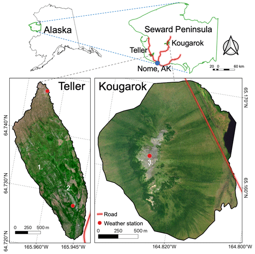
Figure 1 Location and WorldView-2 RGB imagery of the Teller watershed (lower left) and Kougarok Hillslope study sites (lower right). Teller has two weather stations (red dots), located near the top and bottom of the watershed, and the Kougarok Hillslope has one weather station located near the top of the rocky dome. The sites are located on the Seward Peninsula of Alaska, with the HUC12 basins for the Teller watershed and the Kougarok Hillslope shown in green and the Seward Peninsula road system in red (upper right). RGB composite from the eight-band WorldView-2 images obtained on 27 July 2011 (Teller) and 14 July 2017 (Kougarok Hillslope) at 1.5 m resolution downloaded from the DigitalGlobe website (https://www.maxar.com/, last access: 29 July 2022) Imagery © 2011/2017 Maxar. Example of features discussed in the text are denoted on the map as (1) terraces and risers, (2) the Teller watershed stream bed, and (3) the Kougarok Hillslope dome.

The Teller watershed, with elevations ranging from 50 to 300 m, is located nearby the coast and underlain by discontinuous permafrost, with near-surface permafrost adjacent to areas with no permafrost or deep permafrost table locations overlain by a perennially thawed layer (i.e., talik; Jorgenson et al., 2008; Busey et al., 2008; Uhlemann et al., 2021; Léger et al., 2019). Topographic features at the sites include terrace and risers (Fig. 1, no. 1) and stream bed (Fig. 1, no. 2). The streams in the Teller watershed connect to the Sinuk River, about 1 km to the south of the study site. Along the streams, willow shrubs grow, while sedge–willow–Dryas tundra and mixed shrub–sedge tussock tundra–bog dominate the rest of the watershed (Fleming, 2015; Konduri and Kumar, 2021).

The Kougarok Hillslope study site is located inland on the leeward side of the Kigluaik Mountains along a minor drainage of the Kuzitrin River, which flows into the Imuruk Basin. The Kougarok Hillslope is situated on a gently rising upland dome that tops out at an elevation of ∼ 110 m (no. 3; Fig. 1). The site is overlain by an active soil layer containing organic peat and mineral horizons (McCaully et al., 2022), vegetated by alder shrubland, tussock tundra, alder savanna, and rocky areas dominated by dwarf shrubs and lichens (Iversen et al., 2019; Salmon et al., 2016). The site is underlain by permafrost approximately 15–50 m thick, with average active layer thickness of 56 cm (Hinzman et al., 2003).

To obtain spatially consistent and replicable (for different study sites and years) estimates of precipitation falling in each separate year of study, the total winter precipitation (TWP) for each year was estimated based on the ERA5-Land hourly reanalysis product (Muñoz-Sabater et al., 2021), accessed via the Google Earth Engine (https://earthengine.google.com/, last access: 29 July 2022). For each winter, we summed the winter (October to March) precipitation and averaged these totals across the study areas.

2.2 Field observations of snow

From 22 to 31 March 2017 (Teller watershed), 26 March to 5 April 2018 (Teller watershed; Kougarok Hillslope), and 31 March to 7 April 2019 (Teller watershed), end-of-winter snow surveys were carried out at the study sites to collect snow depth and snow density to calculate SWE. SWE measures the amount of water contained within the snowpack and characterizes the hydrological and thermal impacts of snow cover better than snow depth (Jonas et al., 2009; Sturm et al., 2010; Liston and Elder, 2006), which is why we focus on SWE.

We measured snow characteristics in several different ways. Snow depth was captured every 1–15 m using a Snow-Hydro™ GPS snow depth probe (Sturm and Holmgren, 2018). When the snowpack was greater than 130 cm in depth, which is the length of the snow depth probe, an avalanche probe was used to manually measure the snow depth. Snow bulk density was measured with a SWE coring tube, also manufactured by Snow-Hydro™ (reported error of −9 % to 11 %; Dixon and Boon, 2012; Young et al., 2018; López-Moreno et al., 2020). Approximately three to five bulk density samples were taken for each sampling location, with an interval of ∼ 200–300 m between measurements. The snow tube was pressed into the snow until the ground was hit and the depth of the snowpack in centimeters (snow depth) was recorded. After the tube was removed from the snowpack, the snow in the tube was bagged and weighed in grams (snow weight). The cross-sectional area of the snow coring tube (coring tube area) was 30 cm³. Then the snow density (g cm⁻²) was calculated from Eq. (1), as follows:

$$\begin{array}{}\text{(1)}& \text{Snow Density}={\displaystyle \frac{\text{Snow Weight}}{\text{Snow Depth}\times \text{Coring Tube Area}}}.\end{array}$$

Inverse distance weighting (IDW) was used to assign snow density for each of the observed snow depth locations and is a common method for interpolating environmental variables (Franke, 1982; Zimmerman et al., 1999). The IDW method added uncertainty to our SWE estimates since we only collected sparse density measurements. These sparse density measurements ranged over years (Teller) between 0.27 to 0.38 kg m⁻³, with a standard deviation of 0.03 to 0.04 kg m⁻³. SWE (cm) was then calculated from the average of the snow bulk density measurements using Eq. (2), where water density was 0.997 g cm⁻³, as follows:

$$\begin{array}{}\text{(2)}& \mathrm{SWE}=\text{Snow Depth}\times {\displaystyle \frac{\text{Snow Density}}{\text{Water Density}}}.\end{array}$$

SWE was then used as the response variable in our statistical models.

2.3 Site characteristics

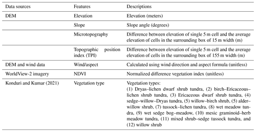
To model snow redistribution, various landscape factors were estimated for topographic, vegetation, and wind characteristics, as described below. An overview of data sources, factors, and descriptions of the factors is given in Table 1.

Table 1 Topography and vegetation data sources. Data sources for the input features are listed on the left, and the description of the features are listed on the right. Note: DEM stands for digital elevation model.

2.3.1 Topography

To evaluate the effects of topography on SWE distributions, a digital elevation model (DEM) was analyzed to estimate elevation, aspect, and slope for each of the study locations. The Teller watershed and Kougarok Hillslope DEMs were derived at a 5 m resolution from interferometric synthetic aperture radar (IfSAR) data available from https://www.usgs.gov/centers/eros/science/usgs-eros-archive-digital-elevation-interferometric-synthetic-aperture-radar (last access: 29 July 2022).

To consider the effects of topography at different spatial scales on SWE distributions, we included a fine-scale microtopography and a topographic position index (TPI) to capture the range of terrain variability across spatial scales. Values are calculated by the difference between the cell and the average elevation of all cells in a surrounding square window of 15 and 155 m width for microtopography and TPI, respectively.

Microtopography in the Arctic can range from submeter (e.g., tussocks) to 1–10 m (e.g., hummocks) in scale (Sturm and Holmgren, 1994). The 15 m microtopography is the finest scale that can be derived using a DEM at 5 m resolution and is equal to the curvature of the terrain (Jenness, 2006). We also consider coarse-scale topographic features defined using TPI, such as terraces and risers, and the stream channel (tens to hundreds of meters). To determine the scale of TPI, we applied a smoothing average window at a range of widths and then picked the optimal width with the best random forest model performance and highest feature importance (see Sect. 4.4; Fig. A1). We derived both of the above-described products from the DEM, following Lopez-Moreno et al. (2009) and Weiss (2001).

2.3.2 Vegetation

Owing to the importance of shrubs for trapping drifting snow in the Arctic (Sturm et al., 2001a; Essery and Pomeroy, 2004; Dvornikov et al., 2015; McFadden et al., 2001), we considered the following different vegetation indicators to reflect types and distributions: vegetation type and vegetation greenness.

Vegetation type was extracted from an updated vegetation map for both study sites (Konduri and Kumar, 2021) and used as a continuous feature ranked for each year and site according to IDW-interpolated SWE. The continuous ranking was applied so that feature importance could be compared across all model features on a consistent basis. The relative rankings from each year and site were then averaged to produce a final ranking used in the models (Table A1).

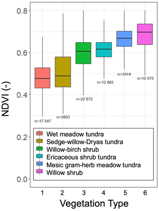
As high-resolution vegetation distribution information is not widely available for most of the Arctic, a normalized difference vegetation index (NDVI) was used to approximate vegetation characteristics. NDVI is indicative of the abundance of photosynthetically active vegetation (Rouse et al., 1974) and is useful to capture the branch abundance, deciduous canopy cover, and maximum height of shrubs in the Arctic tundra landscape (Boelman et al., 2011). NDVI was derived from the eight-band WorldView-2 images obtained on 27 July 2011 at 1.5 m resolution for the Teller watershed and 14 July 2017 for the Kougarok Hillslope. Both images were downloaded from the DigitalGlobe website (https://www.maxar.com/, last access: 29 July 2022). To better understand how the vegetation type was related to NDVI, we binned vegetation types that were present on more than 1 % of the total watershed area, which resulted in six representative categories that encompass the range of wetland species and short shrub and tall shrub vegetation types. We computed statistics and significance to differentiate the NDVI values for those bins using analysis of variance (ANOVA) and Tukey's honest significant difference (HSD) test (Table A1).

2.3.3 Wind

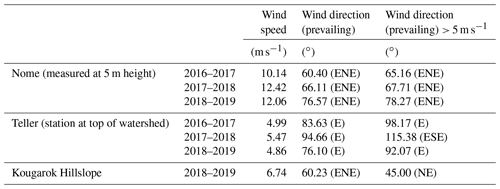
Previous studies showed that snow is usually accumulated on leeward slopes and blown away from windward slopes (Evans et al., 1989; Liston and Sturm, 1998; Winstral et al., 2002; Mott et al., 2011), so we explored whether the prevailing wind would have an impact on the snow distribution. To understand wind patterns, weather stations within the study locations and from the nearby Nome weather station were analyzed (Table A2).

Because faster wind speeds have a greater impact on the redistribution of snow, we considered winter (October to March) wind speeds greater than 5 m s⁻¹ (Table A2; Liston and Sturm, 1998; Berg, 1986; Sturm and Wagner, 2010; Sturm and Stuefer, 2013). At the weather station at the top of the Teller watershed, the prevailing wind direction (wind speeds > 5 m s⁻¹) was the average of the data from the 2016–2017, 2017–2018, and 2018–2019 winters, and at the Kougarok Hillslope weather station, the prevailing wind direction (wind speeds > 5 m s⁻¹) was based on data from the 2018–2019 winter only due to instrument issues in previous years. The prevailing wind direction (wind speeds > 5 m s⁻¹) for each study site was used to represent the exposure of a particular location to wind as a function of aspect (Dvornikov et al., 2015). We divided the prevailing winds into the eight cardinal and ordinal directions (N, NE, E, SE, S, SW, W, and NW), using 45^∘ bins, and then derived a unique wind and aspect factor equation for each directional bin. For the Teller watershed, the prevailing wind direction was 102^∘ E, so the wind and aspect factor (Wf) was calculated using Eq. (3), as follows:

$$\begin{array}{}\text{(3)}& \mathrm{Wf}=-\sin \left(A\right),\end{array}$$

where A is the aspect (Dvornikov et al., 2015; Evans et al., 1989; Liston and Sturm, 1998). For Kougarok Hillslope, the prevailing wind direction was 45^∘ NE, so the Wf was calculated using Eq. (4), as follows:

$$\begin{array}{}\text{(4)}& \mathrm{Wf}=-\cos \left(A\right)-\sin \left(A\right).\end{array}$$

The wind and aspect factor gives positive values for leeward slopes and negative values for windward slopes, since snow is known to blow away from windward slopes and accumulate on leeward slopes (Dvornikov et al., 2015). More details on the wind factors as applied in this work are included in the Appendix and Fig. A2.

3 Methodology

3.1 Modeling

We fit three different types of models, namely linear regression, general additive, and random forest, to quantify the impacts of different factors on snow distribution and characterize the spatial pattern of the snow distribution.

3.1.1 Linear regression model

The linear regression model is shown in Eq. (5), as follows:

$$\begin{array}{}\text{(5)}& y={\mathit{\beta }}_o+{\mathit{\beta }}_{\mathrm{1}}{x}_{\mathrm{1}}+\mathrm{\dots }{\mathit{\beta }}_p{x}_p+\mathit{ϵ},\end{array}$$

where y denotes SWE, and β are the coefficient of factors expressed by the weighted sum of its p features with an error term, ϵ. Linear models are useful in that they produce simple relationships between the response variable and factors, and the factor rankings are easy to interpret. However, relationships between snow distribution and factors may not be linear, and thus linear models may not provide a good result; additionally, linear models are susceptible to correlations between parameters. The linear models were implemented using the Linear Regression class of the Scikit-learn package in Python (Pedregosa et al., 2011).

3.1.2 Generalized additive model

A generalized additive model, or GAM, is a class of statistical models in which the usual linear relationship between the response and predictors are replaced by several nonlinear smooth functions to model and capture the nonlinearities in the data, as follows:

$$\begin{array}{}\text{(6)}& g\left(E_Y\left(y\mathrm{|}x\right)\right)={\mathit{\beta }}_o+f_{\mathrm{1}}\left(x_{\mathrm{1}}\right)+f_{\mathrm{2}}\left(x_{\mathrm{2}}\right)+\mathrm{\dots }+f_p\left(x_p\right),\end{array}$$

where g denotes SWE as a link function that links the expected value to the predictor variables x₁,…xp, which denote smooth, nonparametric functions. This type of model is useful because it allows for nonlinear relationships between SWE and the factors. GAMs are generally easy to interpret, but while they are nonlinear, GAMs still require a fit to a distribution or shape. The GAMs were implemented using the LinearGAM class of the pyGAM package in Python (Servén et al., 2018).

3.1.3 Random forest model

Random forests are based on decision trees, i.e., a series of yes/no questions asked about our data eventually leading to a predicted class (or continuous value in the case of regression; Breiman, 2001). A random forest model is defined by a large number of individual decision trees that operate as an ensemble. Each individual tree in the random forest generates a vote for classes (classification) or mean prediction (regression) of the individual trees, and the one with the most votes is used for the final prediction (Liaw and Wiener, 2002). Random forests are useful in that they are not impacted by correlations in the data, can generally protect against overfitting, and have built-in feature randomization. The drawback of these models is that they can be difficult to control if used in black box mode. The random forests were implemented using the RandomForestRegressor class of the Scikit-learn package in Python (Pedregosa et al., 2011).

3.1.4 Model implementation

For all three model (linear, GAM, and random forest) iterations, SWE, the response variable, was square root transformed to ensure its distribution was normal. Model inputs were also normalized to have a mean of 0 and a standard deviation of 1. We utilized a split sample approach for all models, with a train and test set. Performance metrics for all three statistical models were the coefficient of determination (R²) and root mean squared error (RMSE) on the test set, which were evaluated on the untransformed (squared) model output. Due to the decorrelation effects involved in bootstrapping, the predictive accuracy of random forests is generally robust to collinearity across features (Dormann et al., 2013). However, feature collinearity can still be an issue for determining feature importance (Gregorutti et al., 2017). Prior to modeling, we used variance inflation factors and pairwise correlation coefficients to assess collinearity among features and ensure collinearity was not a significant issue.

We implemented the random forest model using various subsets of the input factors. One implementation, labeled the final model, was trained on data from all years at the Teller watershed and the Kougarok Hillslope combined, with the TWP for each year included as a feature in the model. We also trained the model separately for only the Teller watershed using all years combined (2017–2019), with the TWP included as a feature. In addition, we implemented individual random forest model runs for each year and each site without TWP. The model runs on individual sites and years were also implemented for linear regression models and GAMs so that the performance of the three different statistical models could be compared.

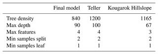
Since the random forest performed the best of the three models and has the most comprehensive feature importance metrics, all testing for model features and hyperparameters was completed with the random forest model. The same features were then applied in the linear model and GAM predictions. Model hyperparameters (tree density, max depth, max features, min samples split, and min samples leaf) were selected using Bayesian search (using the BayesSearchCV function from the Scikit-Optimize package in Python) with eight-fold cross-validation on the training set. The training set was a randomly selected 80 % of full dataset, and the remaining 20 % of the dataset was used for validation. A complete list of the hyperparameters used for the final model and the separate the Teller watershed and the Kougarok Hillslope model runs are given in Table A3.

Using the random forest model, we measured the contribution of each input feature in predicting SWE distribution with both impurity feature importance and permutation feature importance (Louppe et al., 2013). Impurity importance, also known as mean decrease in impurity (MDI) or Gini importance, is proportional to the total number of splits that each feature divides across all trees in the random forest, where features with more splits are more important (Breiman, 2001). While impurity importance is computationally cheap, it is biased towards features with many possible split points, and suffers from overfitting to the training set. Permutation importance, also known as mean decrease in accuracy (MDA), is based on the decrease in model performance when a single feature is randomly shuffled, and more important features result in larger decreases in performance when permuted (Breiman, 2001). Permutation importance is more computationally expensive. We measured permutation importance on the test set. For this study, we analyzed both importance metrics (MDI and MDA) to ensure that the relative feature importance rankings generally agreed.

4 Results

4.1 Meteorological conditions

Meteorological stations located in the study sites (Fig. 1) recorded temperatures of −7.1 ^∘C (the Teller watershed, 2017–2019, including the top and bottom meteorological stations)/−8.1 ^∘C (the Kougarok Hillslope, 2018) during the winter months of October to March, while Nome Airport reported average 2017–2019 winter temperatures of −8.0 ^∘C. From 2017–2019, Nome Airport reported winter temperatures that were slightly warmer than the recent (1981–2010) climatological period (−10.5 ^∘C). Precipitation recorded at Nome Airport climate station indicated that, from October to March, precipitation was 13.3, 28.0, and 25.0 cm, while precipitation, from December to March, at Nome Airport was 7.2, 15.2, and 16.4 cm for 2017, 2018, and 2019, respectively. ERA5 average winter (October to March) total precipitation values are 26.3, 40.3, and 44.9 cm for both the Teller watershed and the Kougarok Hillslope for 2017–2019, respectively. From October to March, the prevailing wind speed and direction for the Teller watershed (top station) were predominantly east–northeast (2017–2019), while Kougarok Hillslope was predominantly northeasterly in 2019 (Table A2; Busey et al., 2017). The Kougarok Hillslope meteorological station experienced issues with its wind sensor in 2018; thus, those values are not reported herein. The wind directions experienced at the study sites are similar to that experienced at Nome Airport (east–northeast). Wind speeds ranged from 4.9 to 6.7 m s⁻¹, which are much lower than wind speeds reported at Nome Airport (10.1 to 12.4 m s⁻¹) in 2017–2019 (Table A2).

4.2 Snow depth, density, and SWE

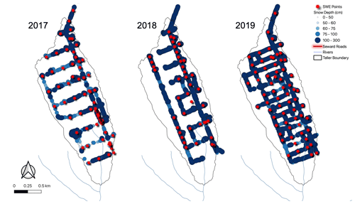
Snow depth was collected at thousands of locations (> 22 000 points), while snow bulk density was measured at hundreds of locations (Table 2; Fig. 2). The number of observations varied from year to year, with the greatest number of snow depth observations being collected in 2017, followed by 2019, and with 2018 having a similar number of observations to 2019 in the Teller watershed. In 2017, the survey was not planned for Kougarok Hillslope, and in 2019, weather concerns prohibited safe travel to the study site. Note that, while the Teller watershed's 2017 survey collected the most points, the 2019 survey was the most spatially extensive (Fig. A3). No snowfall occurred during any of the 2017–2019 end-of-winter snow surveys.

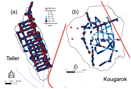
Figure 2 Measured snow depth (cm) and snow density (SWE points) at (a) the Teller watershed (2017–2019) and (b) the Kougarok Hillslope (2018).

Table 2 Teller and Kougarok Hillslope snow depth and density observations and SWE observations and estimates. The coefficient of variation (CV) of the observed variables are in parentheses following the average value.

The average snow depth at the Teller watershed was observed to be lowest in 2017, and similar depths were noted in 2018 and 2019 (109.0 and 106.4 cm, respectively). The average snow depth at the Kougarok Hillslope in 2018 was 75.3 cm. SWE was estimated to be lowest in 2017, lower at the Kougarok Hillslope versus Teller in 2018, and the highest SWE values were recorded in 2019 for Teller (Table 2).

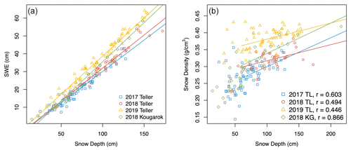
High spatial variability in snow depth was measured (Table 2; Fig. 2). Snow depth ranged from 2 to 300 cm (mean 89 cm; standard deviation (SD) 40 cm; coefficient of variation (CV) 0.45). Snow density measurements ranged from 0.146 to 0.433 g cm⁻³ (mean density of 0.300 g cm⁻³). SWE was strongly correlated with snow depth, with correlation coefficients ranging from 0.95 to 0.97 (Fig. 3a). Snow density positively correlated with snow depth with correlation coefficients from 0.51 to 0.59 (Fig. 3b), with higher correlations deeper than 60 cm. SWE was calculated from snow depth and snow density, as described previously. SWE ranged from 3.3 to 90.5 cm (with mean 27.4 cm and SD 14.6 cm).

Figure 3 Scatterplots of (a) snow depth vs. SWE and (b) snow depth vs. snow density. The linear regressions in panel (b) are for snow depth > 60 cm.

4.3 Topographic, vegetation, and wind features

Topographic features in the study sites illustrate the variation across the landscape (Fig. 4a, b). Elevational gradients are strongest at the Teller watershed, topping out at 300 m, while Kougarok Hillslope's dome-like feature is approximately 100 m. Slopes at the Teller watershed are steeper in the middle of the basin and along the stream banks, while at Kougarok Hillslope slopes are shallower on the west and steeper to the east, with overall more gentle elevational gradients than Teller. TPI highlights dominant features such as the terraces and risers, the stream bank in the Teller watershed, and the top of the dome at the Kougarok Hillslope.

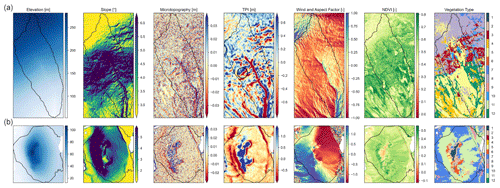
Figure 4 Input features included in the snow models (elevation, slope, microtopography, TPI, wind and aspect factor, and NDVI and vegetation type) for (a) Teller and (b) Kougarok Hillslope. The white areas shown in the Kougarok Hillslope maps are lakes. An open circle on the TPI figure denotes one of the terraces and riser. The vegetation types are (1) Dryas–lichen dwarf shrub tundra, (2) birch–Ericaceous–lichen shrub tundra, (3) Ericaceous dwarf shrub tundra, (4) sedge–willow–Dryas tundra, (5) willow–birch shrub, (6) alder–willow shrub, (7) tussock–lichen tundra, (8) wet meadow tundra, (9) wet sedge bog–meadow, (10) mesic graminoid–herb meadow tundra, (11) mixed shrub–sedge tussock tundra, and (12) willow shrub.

Wind and aspect factors illustrate that the Teller watershed's aspects are largely unidirectional (south–southeast facing), while the Kougarok Hillslope's west hillslope is predominantly south facing, with a north-facing slope on the eastern side over the crest of the dome (Fig. 4a, b). NDVI patterns in July and August are reflective of taller stature shrub patches located across the study sites (Figs. 1, 5; Boelman et al., 2011). Vegetation maps illustrate the differences in the two study sites. The Teller watershed contains low-to-mid-slope willow–birch and willow shrub complexes, with Ericaceous dwarf shrub tundra and wet meadows located in the upper slopes. At the Teller watershed, an ANOVA test of NDVI versus vegetation type (those with > 1 % of total land cover) indicate significant differences ($p<\mathrm{0}.$0001), with the highest NDVI values occurring in willow shrubs (Table A1). Tukey's HSD test showed significant differences among all vegetation types (p<0.0001; Fig. 5). The Kougarok Hillslope's slopes are largely mixed shrub–sedge tussock tundra, with patches of alder–willow shrubs, Dryas–lichen dwarf shrub tundra, birch–Ericaceous–lichen shrub tundra, and willow–birch shrub on the eastern slope where no snow measurements were taken in 2018 (Konduri and Kumar, 2021).

Figure 5 Teller watershed NDVI by major vegetation type. Mesic gram–herb is short for mesic graminoid–herbaceous tundra. Table A1 details each vegetation type.

4.4 Model optimization and testing

Several different tests were undertaken to determine the optimal features used in the final model; we tested this optimization on both sites and for all years. We tested the random forest model to determine the optimal scale of TPI, with a smoothing average window from 55 to 505 m (Fig. A1). The TPI at a scale of 155 m corresponded to the best model performance. Furthermore, the random forest model was used to determine which vegetation features to use in the final model. We tested the model using NDVI, vegetation type as 12 one-hot-encoded categorical features, and vegetation type as a continuous feature ranked by observed SWE, as well as combinations of these three features (Fig. A4). We found that NDVI and the continuous ranking of vegetation type performed the best, so these two features were included in the final model. However, while the spatial pattern of vegetation type improved model performance, the relative order of the vegetation type ranking did not appear to be important, since other randomized rankings performed similarly well (Fig. A4). It should be noted that, while NDVI and continuous vegetation performed the best, the differences across all tests were similar (R² values between ∼ 0.86–0.87).

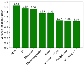
The variance inflation factors of the input features are shown in Fig. 6. Since the variance inflation factors are all well below the accepted threshold of 5 (Karimi et al., 2019), and the largest correlation coefficient between two input variables (0.49 for microtopography and TPI) is well below the accepted threshold of 0.70, collinearity is not expected to severely distort model estimation and predictions (Dormann et al., 2013).

Figure 6 Variance inflation factors for the model inputs.

4.5 SWE prediction

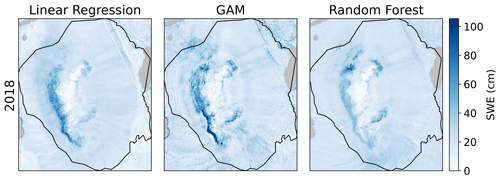
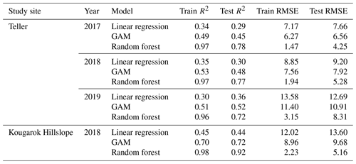
The SWE prediction model results for the linear regression, GAM, and random forest for the individual sites and years are shown in Table 3. In general, linear regression performed the worst (R² ranging from 0.29 to 0.44), random forest performed the best (R² ranging from 0.72 to 0.92), and GAM performed in between the other two models (R² ranging from 0.45 to 0.72). The spatial maps of predicted SWE for the three different models are shown in Fig. A5 for the Teller watershed and Fig. A6 for the Kougarok Hillslope. Because of the success in simulating SWE for the study sites and years using random forest, we focus the remainder of our study on the random forest results to discuss the implications and the driving factors that are ranked to be most important for prediction of SWE in the study sites.

Table 3 Comparison of model performance for linear regression, GAM, and random forest models that are trained on individual years and individual sites.

The random forest model results for training and testing data are given in Table 4. The final random forest model, which includes data from all years and sites, captures approximately 86 % of the variance in SWE and has an RMSE of 5.81 cm on the test set. The scatterplot of predicted and actual SWE measurements of the test set from the final model (Fig. 7) shows a linear trend. In comparison to the y=x line, the linear fit in Fig. 7 shows that the model slightly overestimates low SWE measurements and underestimates high SWE measurements, which could be due to the tendency of random forests to decrease the variance by averaging across many trees.

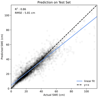
Figure 7 Random forest results of predicted SWE vs. actual SWE for the test set when using all year and site datasets, with a test set of 20 %. R² is equal to 0.86, and the RMSE is equal to 5.81 cm. The solid blue line is a linear fit to the scattered points, and the dashed black line is a y=x line.

Table 4 Random forest results for the training and testing data used to estimate SWE.

We also considered the random forest model developed by using the individual study sites and years as a feature to predict SWE. The iterations of the random forest model where we considered only the Teller watershed and all years performed slightly better than the final model, with an R² of 0.86 and an RMSE of 5.78 cm for the Teller watershed (Table 4). The random forest models trained on individual years and sites ranged in model performance, as shown in Table 4.

In Fig. 8, we illustrate the spatially predicted SWE from the final random forest model for the Teller watershed (2017–2019) and the Kougarok Hillslope (2018). SWE values across the basin reflect the year-to-year variability in the amount of precipitation that fell on the study sites. However, we observe that SWE is variable across the Teller watershed and the Kougarok Hillslope around major landscape features, such as the stream bed and terraces and risers within the Teller watershed. Another location where SWE appears to be higher is just below the dome on the western hillslope in the Kougarok Hillslope. The SWE patterns in SWE also reflect areas of higher NDVI values, where shrubs are identified as darker patches in both the Teller watershed and the Kougarok Hillslope (see Fig. 4).

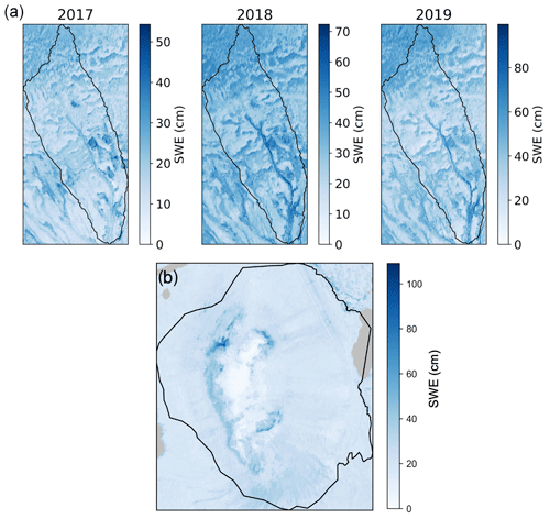
Figure 8 Spatially predicted SWE for the final model for (a) Teller in 2017, 2018, and 2019 and (b) Kougarok Hillslope in 2018. The gray areas in the Kougarok Hillslope map are small lakes. Note that the scales change for each year and study location across the panels.

The spatial error, calculated as the predicted minus the observed for the upper and lower quartiles of error in the random forest SWE prediction, is shown in Fig. A7 for the Teller watershed for each year and Fig. A8 for the Kougarok Hillslope for 2018. In these figures, we observe that the spatial error varies from year to year but is not spatially systematic. Errors are higher in the years where there was lower SWE in the basin, such as in 2018, compared to the lower SWE year of 2017 in the Teller watershed, when the survey resolution was similar (Fig. A3). In 2019, the survey captured higher SWE values but similar CV compared to 2018, while the 2019 survey extent was broader with a finer spatial resolution (Fig. A3). A more detailed consideration of the spatial error in these datasets is beyond the scope of this work.

4.6 Feature importance

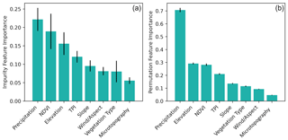
Figure 9 shows the impurity and permutation feature importance results for the final random forest model. Both of the importance metrics provide similar results and the same variable ranking, with the exception of the permutation importance metric ranking elevation as being higher than NDVI and impurity ranking NDVI higher than elevation. TWP is the key primary factor driving SWE distribution. Overall, NDVI, elevation, and TPI are the most important secondary features for predicting SWE distribution at our study sites. Features such as slope, vegetation type, wind/aspect factor, and microtopography are ranked as the least important in SWE prediction.

Figure 9 Random forest feature importance results (where panel a shows the impurity, and panel b shows the permutation) for the final model, with ±1 standard deviation shown by the black error bars.

4.7 SWE correlations between years

Heatmaps that illustrate significant SWE correlations between years 2017–2019 for the Teller watershed are shown in Fig. 10, based on random-forest-modeled SWE trained with data from all years and sites. The weakest correlations are for the years with low (2017) and high (2019) SWE (Pearson correlation coefficient r=0.67), with stronger correlations between the two higher SWE years (2018 and 2019; r=0.89). These correlations tend highlight the consistency in SWE values for the study site across highly variable climate conditions.

Figure 10 Heatmaps of predicted normalized SWE for Teller in 2017, 2018, and 2019, with Pearson correlation coefficients (r) showing significant correlations of SWE among the years. Random forest was trained with data from all years and sites. The color scale represents the density of data points, with dark blue representing areas with the least points and light yellow representing areas with the most points. Areas with fewer than 100 points are not plotted. The solid red line is a line of the best fit using singular value decomposition.

5 Discussion

Changes in snowpack characteristics have important implications for a changing Arctic and are anticipated to be a major driver of ecosystem shifts (Bjerke et al., 2015; Cooper, 2014), water and energy balances (AMAP, 2019; Pulliainen et al., 2020), and biodiversity changes (Niittynen et al., 2018; Riseth et al., 2011). Changes in snow have implications for Arctic communities, where snow may impact many resources (Huntington et al., 2004), and for global climate change (Overland et al., 2019) and carbon cycles (Rogers et al., 2011; Arndt et al., 2020). Thus, understanding how to better model snow distribution and the important features involved in snow distribution is fundamental to improving how we interpret, and plan for, changing Arctic snow in the future (Zhu et al., 2021; Kouki et al., 2022; Mudryk et al., 2020).

5.1 Snow depth, SWE, and density observations

Snow depth and snow density observations collected from two small study sites located on the Seward Peninsula of Alaska comprise an extensive dataset that provides a reliable and representative estimate of the variation in SWE in this region. Snow depth showed high variability at both study sites and years, with a medium level of variability compared to the variability range reported for other Arctic regions (Bruland et al., 2001; Hannula et al., 2016; Dvornikov et al., 2015; Stuefer et al., 2013; Homan and Kane, 2015; Sturm et al., 2010). Compared to snow depth, snow density showed relatively low variability, similar to the findings for other nonforest Arctic areas by Homan and Kane (2015) and Hannula et al. (2016).

Consistent with previous studies (Homan and Kane, 2015; Assini and Young, 2012; Dvornikov et al., 2015; Sturm et al., 2010), there was a high correlation between snow depth and SWE in our study, confirming that SWE is more closely linked to snow depth than to snow density. Sturm et al. (2010) suggested a nonlinear relationship between snow depth and density for a large region of the Northern Hemisphere, while Homan and Kane (2016) did not find any relationship between snow depth and density for a 200 by 240 km region of Alaska's central Arctic slope. Our study showed an overall positive linear correlation between snow depth and density, indicating that snow depth has some control on the snow density for the study sites. However, snow depth and density showed no relationship for shallow snow (< 60 cm), while the linear relationship for deeper snow (> 60 cm) was strongest at most sites and years (with the exception of 2018 at Kougarok Hillslope), consistent with what has been found for a study region consisting of a variety of landscapes in Saskatchewan, Canada (Shook, 1997). The nonlinear relationship between snow depth and density found in the aforementioned work may be due to the fact that the snow surveys documented were conducted for different climate and landscape classes, where snow density was largely controlled by climate (wind and temperature) and landscape classes (such as taiga, tundra, mountain, and coast). On the other hand, a linear relationship between snow depth and density was observed in this study because the climate and landscape in the small study sites are more homogenous.

Finally, when we considered SWE between 3 study years at the Teller watershed site, we found correlations across the years. This is consistent with other research on snow repeat patterns (Sturm and Wagner, 2010; Liston, 2004; Kirnbauer and Blöschl, 1994; Deems et al., 2008; Homan and Kane, 2015; Woo and Young, 2004; König and Sturm, 1998; Rees et al., 2014; Dozier et al., 2016; Erickson et al., 2005; Winstral and Marks, 2014), indicating that there are driving factors that influence snow distribution consistently across the year-to-year snow variability (i.e., high and lows).

5.2 SWE modeling and prediction

The patterns of our SWE maps illustrate the power of utilizing random forest tools over linear methods of estimating SWE distributions (e.g., Broxton et al., 2019; Revuelto et al., 2020; King et al., 2020). When compared to linear and GAM models, we found that random forests significantly outperformed those models. This is mostly likely due to the fact that SWE distributions are controlled by highly nonlinear interactions between topography and vegetation characteristics; thus, the flexibility offered by the random forest model can more accurately account for these interactions. While GAM models have been applied successfully to estimate nonlinear relationships in snow depth (López-Moreno and Nogués-Bravo, 2005) in the Spanish Pyrenees, they were not as successful at predicting SWE in our study compared to the random forests model. Random forest also allowed us to test different hypotheses of configurations for the model, clearly determining the success of those configuration and features combinations.

5.3 Features impacting snow distribution

There were two different techniques measuring importance in the random forest model that gave similar results, i.e., that the greatest controls on SWE were TWP (i.e., precipitation representing climate variability), followed by the key secondary factors NDVI, elevation, and TPI. These results in general were consistent with those in previous studies in terms of how those factors affected snow distribution in the Arctic, i.e., more snow accumulated in areas with tall shrubs (Sturm et al., 2001b, a; Sturm and Wagner, 2010; Sturm et al., 2005), at higher elevations (Dozier et al., 2016; Homan and Kane, 2015), and within features such as the stream bed and at the bottom of terraces and risers (Gisnås et al., 2014; Grünberg et al., 2020).

NDVI in our study tend to reflect the taller shrub patterns present in the landscape. In this work, we applied the NDVI estimate from July, near the end of the vegetation growth period, which has been corroborated in previous work to be the peak NDVI (Boelman et al., 2011). Although vegetation type in our work was slightly less important than NDVI in our modeling overall, we found taller stature shrub types had higher NDVI values. Vegetation type has been noted to play a primary role in end-of-winter snow depth patterning and is also strongly related to variability in winter and spring soil temperatures in the Arctic (Grünberg et al., 2020). Because of the strong feedbacks between snow, shrubs, and climate (Boike et al., 2019; Sturm et al., 2001a, b), this finding indicates the importance of understanding vegetation dynamics in sub-Arctic regions.

Interestingly, in a study examining snow depth distribution using random forests across a low-relief high Arctic site located in Nunavut, Canada, Meloche et al. (2022) indicate that vegetation ecotype was the least important factor in snow depth distributions. This was largely explained by the fact that ecotypes are correlated with topographic parameters (such as TPI), and this correlation led to low feature importance in the models. When the authors removed the TPI parameters in their modeling, ecotype became more important, while model skill was reduced. Our study differs from this work in that it was undertaken using SWE, carried out in a sub-arctic region with moderate relief, and performed using a vegetation index (NDVI) to directly represent shrub influence on the snow, rather than utilizing an ecotype approach. Hence, the ecotype method applied in conjunction with the random forests approach by Meloche et al. (2022) reduced the influence vegetation had on snow distribution, which made vegetation appear unimportant as a factor in the snow depth distributions. Instead, as our research indicates, vegetation characteristics are an important secondary driving variable in snow distributions at Arctic sites.

Our results showed that elevation effects are a dominant factor driving snow distributions at our study sites. We observe an increase in SWE at higher elevations at the Teller watershed due to a slight orographic effect, consistent with the study for a small high-Arctic glacier Svenbreen (Małecki, 2015). However, an apparent orographic effect also occurs because wind blows snow from outside the catchment into the upper wetland meadow. Homan and Kane (2015) discussed a relationship between snow and elevation below specific elevation bands, above which snow is controlled by moisture availability; however, the Teller watershed's maximum elevation (300 m) is above the value, suggesting that the threshold may change due to other local or regional factors. However, we also observed a decrease in SWE at the top of the Kougarok Hillslope, where snow is removed completely from the upper windswept top (Assini and Young, 2012; Shook and Gray, 1996; Homan and Kane, 2015).

TPI in our model was found to be the third most important variable, indicating the importance of coarse-scale features in the sub-Arctic landscapes of the Seward Peninsula. These coarse-scale features, including stream banks and terrace risers, are areas of topographic variability where shrubs grow and snow accumulates. Thus, they act as hydrology focal points in the basins where higher enhanced soil moisture and soil warming, and associated increased ecological productivity, can occur (Westergaard-Nielsen et al., 2017). These are also features that act to entrain snow distributed by wind. Indeed, recent research into snowdrift landscape patterns in the Arctic have found that wind transports snow into coarse-scale features called drift traps, including stream beds, lake features, outcrop features, and more. These drift traps contain as much as 40 % of SWE found on the landscape and play a significant role in the distribution of snow in the Arctic (Parr et al., 2020). Meloche et al. (2022) also found that topographic parameters of TPI and upwind slope index were the two most important features in the random forest modeling of snow depth distribution for a low-relief high-Arctic basin.

In our study, microtopography was found to be one of the least important factors driving snow. However, microtopographic patterns were highly correlated with curvature. In research from Dvornikov et al. (2015), curvature was found to have a dominant control on the snow depth at a shrub tundra area in the central Yamal Peninsula, and there was a positive correlation between shrub heights, and snow depth was observed for convex slopes. However, research in fine-scale polygonal tundra sites of the high Arctic, microtopography was found to be an important control on snow (Wainwright et al., 2017). Our study utilized DEMs with a 5 m resolution, with the caveat that microtopography features dominant in this landscape (e.g., drainage paths and terraces) range from centimeters to meters in scale. Thus, we require finer-scale DEM sources to investigate this in more detail (Adams et al., 2018; Harder et al., 2020; Revuelto et al., 2021).

5.4 Future work

The ability to model and predict SWE is important on a number of fronts. First of all, we intend to utilize these findings to compare them with physics-based modeling efforts and for future machine-learning efforts. Our models are being used for investigation of subgrid SWE variability in E3SM's ELM (Caldwell et al., 2019; Bisht et al., 2018), along with the investigation of ecosystem-type constructs for upscaling of SWE.

Several of our findings require further investigation to clearly understand their importance for snow distribution. For example, NDVI was an important parameter in our model predicting snow distribution, but we do not know which vegetation characteristics (e.g., shrub height, density, allometry, or wetness) NDVI represents, making it harder to extrapolate the importance of vegetation characteristics for snow distribution at other sites across the Arctic and sub-Arctic. Furthermore, there are likely relationships between TPI and NDVI that should be investigated, including at smaller spatial scales. We are also considering the application of more advanced wind functions (Winstral et al., 2002) in our models and implementing a physically based wind model for comparison and testing against our statistical models (Crumley et al., 2021; Liston, 2004).

We used multiple study sites with varying characteristics across multiple climate years to develop our snow distribution estimates. Because of this unique dataset, we were able to develop robust machine-learning-based models that we hypothesize are representative of broader SWE patterns across time and space. However, these theories require additional validation at more locations. This hypothesis testing will be incorporated into current and future work that will be carried out using broader observations of SWE and snow depths that can be compared with other remote sensed SWE data products.

6 Conclusions

The extensive snow depth and density dataset from this study is of high value for calibrating and validating physically based models of snow distribution. As the patterns of snow distribution for a given location are similar from year to year, the spatial patterns of snow distribution characterized in this study can be used to represent the typical patterns of snow distribution and model the relative spatial patterns of snow distribution for other years for the study sites and across the region. Linear relationships between snow depths greater than 60 cm and snow density revealed homogeneity in the study sites. Snow depth, on the other hand, varied considerably with strong linear relationship to SWE.

We found that random forest models could simulate the SWE distribution most accurately when compared to linear and GAM model approaches, and we were able to simulate the distribution of SWE across the landscape of these small sub-Arctic study sites. The results of the statistical model are useful for understanding the surface water hydrology during spring snowmelt and explaining differences in permafrost distribution and active layer depth, which have an impact on groundwater hydrology. Using the machine-learning-based model random forest, we were able to determine which factors – in addition to precipitation – were most important at these sub-Arctic study sites for SWE distribution. These factors were NDVI, followed by two topography indexes, elevation, and TPI.

Appendix A: Wind equations

The two wind equations in the current study were derived similarly to the wind equation found in Dvornikov et al. (2015). The purpose of the wind equations is to establish an index using positive and negative values based on the topography–wind relationship. First, we used meteorological station data to calculate an average prevailing wind direction for the winter months. Second, we used the corresponding wind equation to assign positive values to the leeward side of topographical features (where wind loading or drifting of snow is likely) and negative values to the windward side of topographical features (where wind scour of snow is likely).

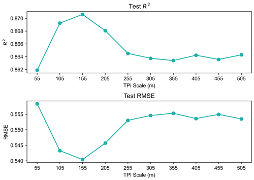
Figure A1 Random forest model performance for model runs using a range of TPI scales. The model performance is optimized when the TPI scale is 155 m.

To derive our wind equations, we divided the wind rose into eight cardinal directions by ±22.5^∘ increments, i.e., N, NE, E, SE, S, SW, W, and NW. The eight possible wind equations that correspond to the eight cardinal directions are listed below, along with the range of values associated with each equation. We determined that the coefficients from Dvornikov et al. (2015) simply added a scaling factor to the wind equation values and were not necessary for our results.

We chose two wind equations (NE and E) for our study area based on the prevailing winter wind direction for each year (Fig. A2).

•  

  N, where Wf(x) = −cos(x) and range = −1 to 1

•  

  NE, where Wf(x) = −cos(x) − sin (x) and range = −1.414 to 1.414

•  

  E, where Wf(x) = −sin(x) and range = −1 to 1

•  

  SE, where Wf(x) = cos(x) − sin (x) and range = −1.414 to 1.414

•  

  S, where Wf(x) = cos(x) and range = −1 to 1

•  

  SW, where Wf(x) = cos(x) + sin (x) and range = −1.414 to 1.414

•  

  W, where Wf(x) = sin(x) and range = −1 to 1

•  

  NW, where Wf(x) = −cos(x) + sin (x) and range = −1.414 to 1.414.

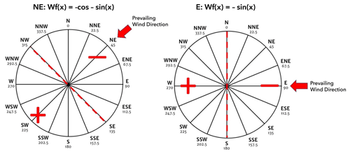
Figure A2 The prevailing wind directions (NE and E) calculated from meteorological station data and the corresponding wind equations applied in this study.

Figure A3 Teller snow depth and SWE measurements for each year of the survey.

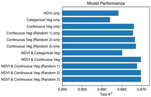
Figure A4 Random forest model performance for model runs using various combinations of vegetation features. The categorical vegetation uses the vegetation types shown in Fig. 4. The continuous vegetation is a ranking ordered by which vegetation type has higher SWE. The continuous vegetation ranking is also randomized in three different ways to determine if the ranking order is important.

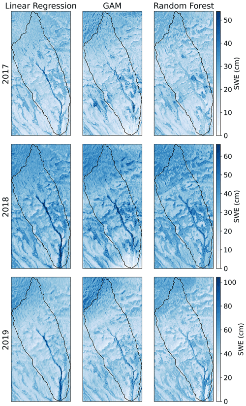
Figure A5 All three statistical models trained on individual years at Teller. The scale of the SWE changes from year to year, depending on the annual snowfall.

Figure A6 All three models trained on single year (2018) at Kougarok Hillslope.

Table A1 Vegetation classes ranked by observed SWE from lowest SWE (1) to highest SWE (12) at Teller. All binned values are significantly different from each other.

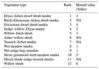
NA in binned values indicates that the vegetation types comprised <1 % of total area at Teller.

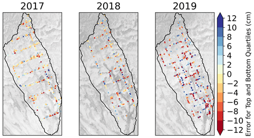
Figure A7 Spatial error (predicted minus observed) for the uppermost and lowermost quartiles of error in the random forest SWE prediction for Teller.

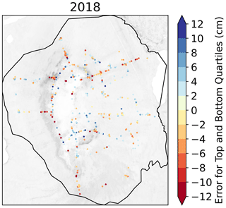
Figure A8 Spatial error (predicted minus observed) for the uppermost and lowermost quartiles of error in the random forest SWE prediction for the final model at Kougarok Hillslope. The error is not distributed systematically through space.

Table A2 Average winter (October–March) wind speed and prevailing direction.

Table A3 Hyperparameters for the random forest model.