the Creative Commons Attribution 4.0 License.
the Creative Commons Attribution 4.0 License.
 | 24 Jan 2022
Retrieval and parameterisation of sea-ice bulk density from airborne multi-sensor measurements
Stefan Hendricks
Robert Ricker
Luisa von Albedyll
Thomas Krumpen
Christian Haas
Knowledge of sea-ice thickness and volume depends on freeboard observations from satellite altimeters and in turn on information of snow mass and sea-ice density required for the freeboard-to-thickness conversion. These parameters, especially sea-ice density, are usually based on climatologies constructed from in situ observations made in the 1980s and earlier while contemporary and representative measurements are lacking. Our aim with this paper is to derive updated sea-ice bulk density estimates suitable for the present Arctic sea-ice cover and a range of ice types to reduce uncertainties in sea-ice thickness remote sensing. Our sea-ice density measurements are based on over 3000 km of high-resolution collocated airborne sea-ice and snow thickness and freeboard measurements in the western Arctic Ocean in 2017 and 2019. Sea-ice bulk density is derived assuming isostatic equilibrium for different ice types. Our results show higher average bulk densities for both first-year ice (FYI) and especially multi-year ice (MYI) compared to previous studies. In addition, we find a small difference between deformed and possibly unconsolidated FYI and younger MYI. We find a negative-exponential relationship between sea-ice bulk density and sea-ice freeboard and apply this parameterisation to one winter of monthly gridded CryoSat-2 sea-ice freeboard data. We discuss the suitability and the impact of the derived FYI and MYI bulk densities for sea-ice thickness retrievals and the uncertainty related to the indirect method of measuring sea-ice bulk density. The results suggest that retrieval algorithms be adapted to changes in sea-ice density and highlight the need of future studies to evaluate the impact of density parameterisation on the full sea-ice thickness data record.
- Article
(7934 KB) - Full-text XML
- BibTeX
- EndNote


Sea ice affects the heat, moisture, and energy exchange between the ocean and the atmosphere; therefore monitoring the state of sea ice is crucial for understanding the current climate, how it may evolve, and what its impact may be (e.g. Stroeve and Notz, 2018). Observing sea-ice thickness and volume over decadal periods relies on freeboard measurements by satellite laser and radar altimeters. The conversion of freeboard to sea-ice thickness requires information of snow mass as well as the density of the sea-ice layer. Observations of both input parameters are sparse, and the unknown spatial and temporal variability and trends of snow mass and sea-ice density directly translate into the uncertainty of the sea-ice thickness data record (Giles et al., 2007; Kwok, 2010; Zygmuntowska et al., 2014; Landy et al., 2020). The current uncertainties related to sea-ice thickness and volume retrievals are sometimes deemed too large for modelling comparisons (SIMIP Community, 2020), and therefore improved accuracy of sea-ice thickness is highly desired (Duchossois et al., 2018). At the beginning of the era of satellite altimetry, starting with the European Remote Sensing satellite ERS-1 mission of the European Space Agency (ESA) in 1993, multi-year ice (MYI, ice that has survived at least two melt seasons) covered about 40 % of the late-winter Arctic and already showed signs of reduction in areal coverage. Since then, Arctic sea ice has undergone rapid change due to the warming climate, resulting in a thinner and younger ice cover (Maslanik et al., 2011; Comiso, 2012; Meier et al., 2014; Stroeve and Notz, 2018). Toward the end of the 2010s, MYI continued to decline and constituted barely 10 % of the Arctic sea-ice extent while the relative extents of the thinner first-year ice (FYI, ice that has not undergone a melt season) and second-year ice (SYI, ice that has survived one melt season) have increased (Stroeve and Notz, 2018).
Due to the lack of spatially and temporally representative snow observations, sea-ice thickness retrieval methods are based on, for example, monthly snow climatologies or modelled reconstructions from reanalysis. Currently the most widely used source for snow mass information is the snow climatology in Warren et al. (1999) (hereafter W99) using data collected during the Soviet North Pole drifting stations in 1954–1991. However, the stations were located exclusively on MYI and thus introduce a bias. In response to the declining MYI, many satellite data products of Arctic sea-ice thickness are derived by using a modified W99, where the snow depth values are halved on ice that corresponds to FYI (Kurtz and Farrell, 2011; Sallila et al., 2019). In attempts to overcome the mismatch between the pre-1990s climatology and the shift toward FYI-dominated, thinner, and younger Arctic sea ice, a number of new snow depth products have emerged in recent years. Descriptions of the different snow depth products currently available can be found in the inter-comparison study of Zhou et al. (2021, and references therein) and in broad outlines below. W99 was complemented with data from airborne Sever expeditions covering in particular FYI in the shelf seas of the Eurasian Russian Arctic in late winter (March–May) in 1959–1986. Other approaches have utilised atmospheric reanalysis data to model a reconstruction of snow on Arctic sea ice in varying spatial and temporal resolutions. Snow depth has been derived using brightness temperatures from passive microwave satellites as well as combining dual-altimetry freeboard information from Ku-band and Ka-band or laser satellite altimeters. Some constraints of the current products will be reduced by near-real-time dual-altimetry acquisitions, such as the resonance of the CryoSat-2 and ICESat-2 satellite orbits (CRYO2ICE) since July 2020, and future single-platform dual-frequency satellite missions like the Copernicus Polar Ice and Snow Topography Altimeter (CRISTAL) mission by ESA (Kern et al., 2020) with a launch planned in 2027. Similar efforts to bring sea-ice density values up to date should be taken as underlined in, for example, Quartly et al. (2019).
Sea ice is a multi-phase substance consisting of solid ice, liquid brine, and gas (air) bubbles with densities and relative amounts depending on temperature (Timco and Frederking, 1996). Calculated from its molecular structure, density of pure ice is 916.8 kg m−3 (Pounder, 1965), while liquid saline water increases and air inclusions decrease the sea-ice bulk density (weight per unit volume including voids and enclosed water). Through processes like brine expulsion, gravity drainage, and meltwater flushing, sea ice is desalinated over time as pore space previously occupied by highly saline brine is replaced by sea water and air, resulting in decreased density of MYI (Petrich and Eicken, 2017). Several studies have demonstrated the rather large range of values for sea-ice density despite little brine drainage and with differences in respect to the waterline and ice type: above the waterline FYI density is 840–910 kg m−3 and MYI density is 720–910 kg m−3, whereas below the waterline ice is saturated by sea water and has a density of 900–940 kg m−3 less dependent on its age (Timco and Frederking, 1996; Timco and Weeks, 2010; Pustogvar and Kulyakhtin, 2016). Especially with satellite altimetry applications in mind, Alexandrov et al. (2010) derived a density of 916.7±35.7 kg m−3 for FYI using the drill-hole data set of airborne Sever expeditions concentrated in the shelf seas of the Eurasian Russian Arctic in the 1980s and a density of 882±23 kg m−3 for MYI as a weighted average of the layers above and below the waterline using values from literature. The values by Alexandrov et al. (2010) (hereafter A10) are the most commonly used in sea-ice thickness retrieval algorithms (Sallila et al., 2019). It has to be noted that the majority of the density measurements originate from Arctic sites, which is also the case in our study. Different properties and processes of Antarctic sea ice could lead to different density values.
Accurate and representative measurements of sea-ice density using traditional techniques are temporally and spatially limited. Most of them require coring or cutting out pieces of ice, such as the mass/volume, displacement (submersion), or specific gravity techniques, making them susceptible for inaccuracies through brine drainage and imprecise volume of the samples (Timco and Frederking, 1996). This can be avoided by carefully recording sea-ice thickness and freeboard, e.g. with drill-hole measurements, in addition to the snow depth atop and calculating the sea-ice bulk density assuming isostatic equilibrium and densities of snow and sea water. However, significant error may be introduced locally where sea ice is not isostatically compensated due to lateral stresses, e.g. close to pressure ridges (Timco and Frederking, 1996). Previous parameterisations of sea-ice density include the effective freeboard approach (snow depth converted to ice thickness using their density ratio) by Ackley et al. (1976) using drill-hole measurements from 400 m of profile lines on MYI in the Beaufort Sea and a parameterisation based on ice floe thickness by Kovacs (1997) utilising 17 FYI and 4 MYI sea-ice cores from the Beaufort Sea. Neither of these parameterisations has been widely used. Moreover, the multi-phase nature of sea ice is an ongoing challenge for modelling approaches (Hunke et al., 2011). There is a definite need for evaluating sea-ice density because there is no density climatology available representing the current state of sea ice, nor is it possible to observe density by satellites from space.
Simultaneous, collocated, and preferably single-platform measurements of the key parameters of the entire sea-ice–snow layer covering a wide range of ice types and conditions on regional scales are required to decrease the uncertainties related to the conversion of freeboard to sea-ice thickness. Since 2017, a unique sensor configuration on the Alfred Wegener Institute's (AWI) IceBird winter campaigns combines airborne laser, radar, and electromagnetic induction sounding instruments, making it now possible to measure them on a single platform. In this paper, we present high-resolution data of simultaneous airborne sea-ice thickness, freeboard, and snow depth over late-winter Arctic sea ice from the AWI IceBird campaigns in 2017 and 2019. Observing the locations of the air–snow, snow–ice, and ice–water interfaces in the sea-ice system along survey tracks allows us to estimate sea-ice bulk density that also serves as a consistency check between the sea-ice thickness, freeboard, and snow depth measurements. Our objective is to derive an updated parameterisation of sea-ice bulk density based on a single variable observable from space. The resulting parameterisation should be suitable for the present Arctic sea-ice cover including the densities of deformed sea ice, which, if unconsolidated, can deviate even more strongly from the density of solid ice.
2.1 Aircraft campaigns
The AWI IceBird program (2020, see reference list for a link to web page) is a series of airborne campaigns carried out using the institute's two Basler BT-67 research aircraft Polar 5 and 6 (Alfred-Wegener-Institut Helmholtz-Zentrum für Polar- und Meeresforschung, 2016) to measure Arctic sea ice and its change since 2009. The campaigns operate from airfields extending from Longyearbyen in Svalbard to Utqiaġvik (Barrow) in Alaska and coincide closely with the Arctic sea-ice summer minimum (August) and winter maximum (April). The primary scientific instrumentation on the aircraft includes an electromagnetic (EM) induction sounding instrument (EM-Bird) to measure total (i.e. ice + snow) thickness, an airborne laser scanner (ALS) for surface topography and freeboard measurements, a microwave radar to measure snow depth, and an infrared radiation pyrometer to record surface temperature (Fig. 1). We describe each instrument in the following sections. The low altitude of 200 ft (≈60 m) and slow speed of 110 kn (≈60 m s−1) during the nominal surveys are beneficial for high-resolution data acquisition.
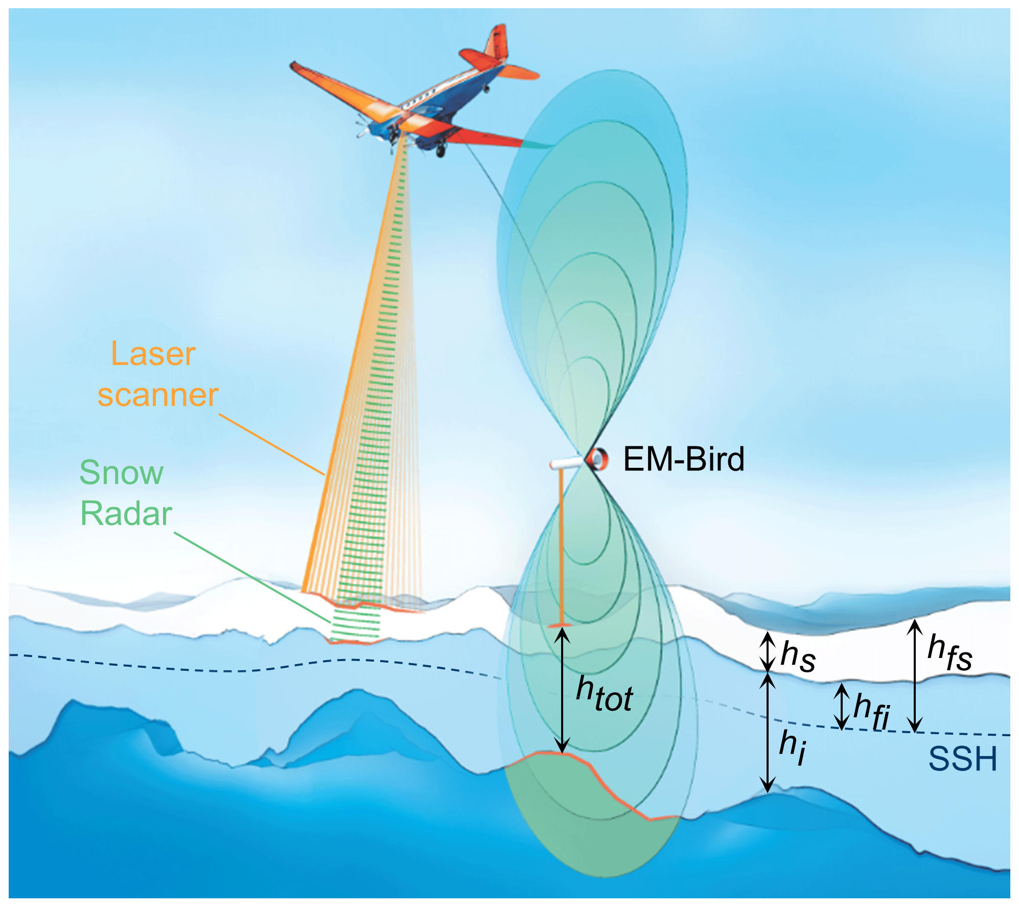
Figure 1Sketch of the IceBird sea-ice campaign setup with the EM-Bird (black text), the laser scanner (orange), and the Snow Radar (green). Different components of sea ice are highlighted in the cross section: total (ice+snow) thickness (htot), snow depth (hs), sea-ice thickness (hi), sea-ice freeboard (hfi), and snow freeboard (hfs). SSH stands for local sea-surface height, depicted by the blue dashed line. Adapted with annotations from the graphic by Alfred Wegener Institute/Martin Künsting CC-BY 4.0.
In this study, we used data collected during the IceBird winter campaigns in early April of 2017 and 2019 (Table 1, Fig. 2), utilising the unique data set of simultaneous total thickness, snow freeboard, and snow depth measurements. From 2017, we used measurements from four survey flights that took place over the Beaufort and Chukchi seas as part of the Polar Airborne Measurements and Arctic Regional Climate Model Simulation Project (PAMARCMiP; Haas et al., 2010; Herber et al., 2012). From 2019, we included five survey flights that covered regions in the Lincoln Sea and the Arctic Ocean in addition to an overlap with the measurements in the Beaufort Sea in 2017.
Table 1IceBird surveys in 2017 and 2019 in the focus of this study (Fig. 2) together with their total lengths and instrument retrieval rates.

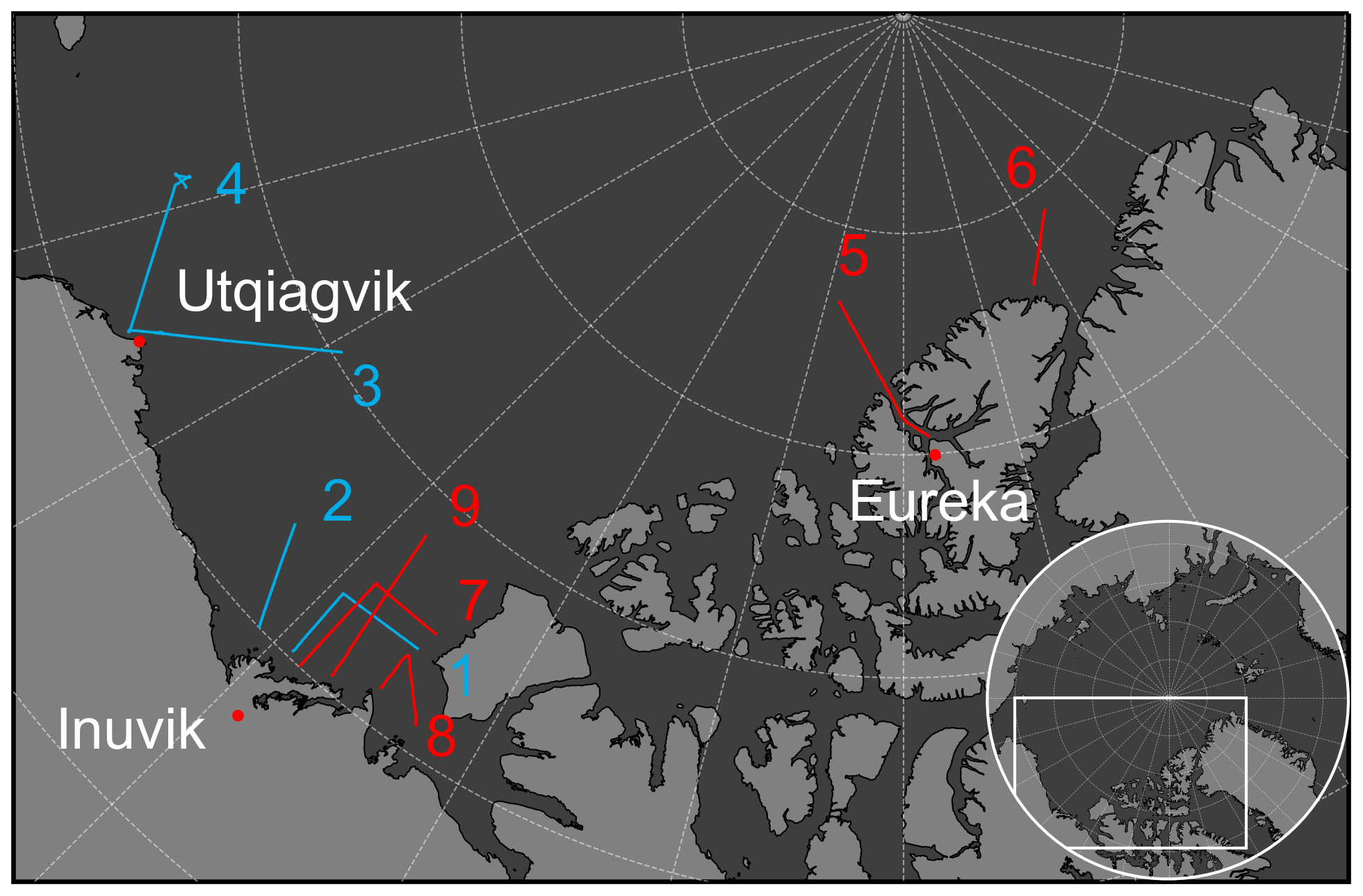
Figure 2IceBird surveys in 2017 (blue) and 2019 (red) in the focus of this study. The numbering corresponds to the individual surveys listed in Table 1.
2.2 Sea-ice thickness
We measured total (ice + snow) thickness of sea ice (htot) using the towed EM induction sounding instrument, the EM-Bird, suspended below the aircraft 10–20 m above the sea-ice surface (Haas et al., 2009) as illustrated in Fig. 1. The EM-Bird utilises the contrast between resistive snow and ice layers and conductive sea water by transmitting an EM field that induces eddy currents only in the latter (Kovacs and Morey, 1991; Haas et al., 1997). The EM-Bird measures the phase and amplitude of a secondary EM field induced by those eddy currents in relation to the primary field. The phase and amplitude of the secondary field depend on the distance between the instrument and the ice–water interface and decrease negative exponentially with increasing distance. Subtracting the instrument height above the surface, measured by an integrated laser altimeter, from the distance to the sea water gives the total thickness (Haas et al., 2009, 2021). Sea-ice thickness (hi) was derived by subtracting snow depth from total thickness (see Sect. 2.4). The EM-Bird sampling rate was 10 Hz, which translated to 5–6 m point spacing at the nominal survey speed. Approximately every 15–20 min brief ascents to more than 100 m were carried out to monitor the sensor drift during post-processing (Haas et al., 2009). Comparison to drill-hole measurements over level ice have indicated an accuracy of 0.1 m, whereas ridge peak thicknesses are generally underestimated by up to 50 % as a result of mass-conserving averaging effects within the approximately 40 m diameter footprint of the instrument (Pfaffling et al., 2007; Haas et al., 2009). For our analysis, we disregarded measurements of total thickness (i) less than the instrument accuracy of 0.1 m and (ii) less than the mean snow freeboard or snow depth and (iii) where the surface temperature was above −5 ∘C within the footprint of the instrument to avoid open or newly frozen leads with total thickness below the accuracy of the EM-Bird (see Sect. 2.4 and 2.5.1).
2.3 Freeboard
The near-infrared (1064 nm), line-scanning Riegl VQ-580 airborne laser scanner (ALS) measured ellipsoidal elevations of ice surfaces with a 60∘ field of view, resulting in a swath width approximately equal to the aircraft's altitude above ground (nominally ≈60 m). We obtained freeboard from the ALS data by subtracting the local sea-surface height from the ice surface elevations. The height of the sea surface along the flight track is sporadically observed by the ALS at open fractures (leads) of the sea-ice cover or newly frozen leads with negligible freeboard, and we manually selected the corresponding elevations. The spacing of leads was diverse and depended on the ice regime varying between less than 10 km (FYI) and potentially more than 30 km (densely packed MYI). We subtracted the mean sea surface (DTU15 MSS; Andersen et al., 2016) from the surface elevations to remove large-scale variations and reduce interpolation errors before applying a spline interpolation between the sea-surface height tie points along the flight track. Data before the first lead detection and after the last lead detection during a survey flight were discarded to avoid extrapolation errors. Subtracting the interpolated sea-surface height from the ice elevations results in snow freeboard (hfs), as the elevation measurement of the ALS always includes the snow layer (Fig. 1). Sea-ice freeboard (hfi), i.e. the location of the snow–ice interface in relation to the local sea level, was derived by subtracting snow depth from snow freeboard (see Sect. 2.4). We then interpolated the obtained point cloud data of snow freeboard onto a regular grid with a 0.25 m resolution. Freeboard uncertainties are dominated by the accuracy of the interpolation of the instantaneous sea surface anomaly that depends on the abundance of leads. Therefore, especially regions with packed MYI and low lead density are associated with high uncertainties (Ricker et al., 2016), and we manually masked out such areas. Supervising the along-track interpolation, we estimated an overall uncertainty of 0.1 m. For each total thickness measurement, we calculated the corresponding mean snow freeboard within the EM-Bird footprint (Fig. 3).
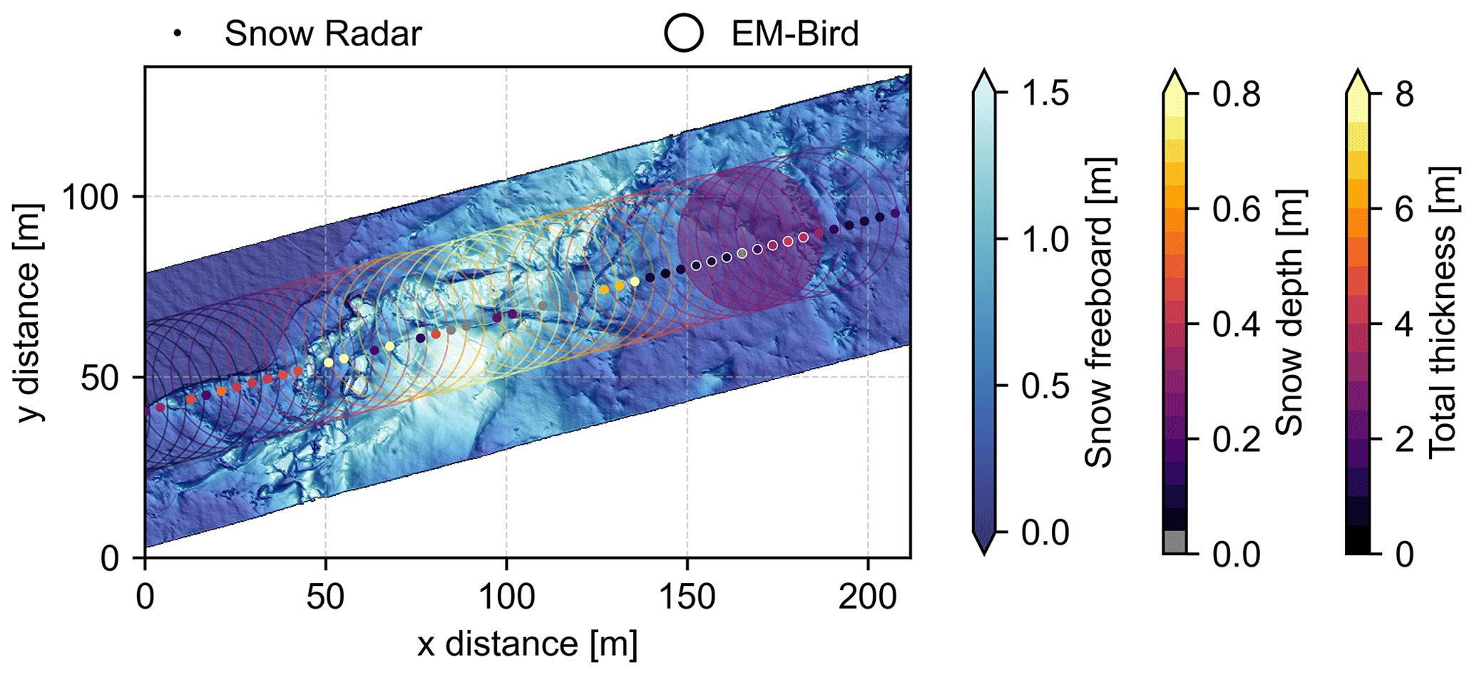
Figure 3Example of the primary data sets: the bluish colours show the gridded 0.25 m resolution swath of snow freeboard (hfs) measured by the ALS; the small filled circles are the snow depth estimates (hs) from the Snow Radar, where the diameter of the circle corresponds to the theoretical smooth surface cross-track footprint of the radar; and the large open circles represent the total (ice+snow) thickness measurements (htot) from the EM-Bird in their respective footprint size. One EM-Bird footprint on the right is highlighted (filled transparent colour) to demonstrate the averaging of snow depth estimates (white outlines) and freeboard. A refrozen lead can be seen in the upper left corner of the figure and a pressure ridge in the middle.
2.4 Snow depth
We used an ultra-wideband (2–18 GHz) frequency-modulated continuous-wave (FMCW) quad-polarised microwave radar, hereafter Snow Radar, to measure snow depth on sea ice (hs). The radar was developed by the Center of Remote Sensing of Ice Sheets (CReSIS) at the University of Kansas, and similar radars have been operated as part of NASA's Operation IceBridge (OIB) since 2009 (MacGregor et al., 2021). Similar to the ALS, the Snow Radar transmitter and receiver antennae were mounted under the aft floor of the aircraft looking nadir (Fig. 1). Due to the broad bandwidth of the radar, its range resolution in snow was 1.14 cm when assuming a snow density of 300 kg m−3. The low altitude and slow speed of the IceBird surveys resulted in an approximately 4–5 m sample spacing and a theoretical smooth surface footprint diameter of only 2.6 m across-track and 1.0 m along-track (Fig. 3). A detailed description of the radar is given in Yan et al. (2017) and Jutila et al. (2022).
To calibrate the raw Snow Radar data, we used a workflow described in Jutila et al. (2022) including coherent noise removal and system impulse deconvolution. Using an open-source Python package pySnowRadar (King et al., 2020a), we detected air–snow and snow–ice interfaces with the algorithm by Jutila et al. (2022) that is based on a pulse peakiness approach by Ricker et al. (2014) used in satellite altimetry. Taking into account the decreased wave propagation speed in snow by assuming a snow density, the distance between the identified interfaces determined the snow depth estimate. In post-processing, we filtered out values which were acquired during the EM-Bird calibration manoeuvres with a simple altitude threshold of 100 m and when the absolute roll or pitch of the aircraft exceeded 5∘. Additionally, for each snow depth estimate we calculated a surface topography estimate (htopo) as the difference between the 95th and 5th percentiles of the ALS surface elevation data within the radar footprint to disregard potentially erroneous snow depth estimates over heavily deformed sea ice using a threshold value of 0.5 m (Jutila et al., 2022).
A validation exercise over level, landfast FYI yielded a negligible mean bias of 0.86 cm, which was below the radar resolution and within the accuracy of the ground truth data, and a root-mean-square error (RMSE) of 6.9 cm for the radar-derived snow depth estimates (Jutila et al., 2022). For each total thickness measurement, we calculated the corresponding mean snow depth requiring at least five valid snow depth estimates within the EM-Bird footprint (corresponds to approximately 50 % of the values; Fig. 3). The averaging reduced the error by a factor of , where N is the number of averaged estimates. We disregarded averaged snow depth values where the surface temperature within the EM-Bird footprint was above −5 ∘C and where the mean snow freeboard was less than the mean snow depth (negative sea-ice freeboard) to avoid potentially erroneous snow depth retrievals due to changes in the dielectric properties of snow induced by liquid water (Barber et al., 1995; Kurtz and Farrell, 2011; Kurtz et al., 2013; Rösel et al., 2021). However, it has to be noted that the studies of Kurtz and Farrell (2011), Kurtz et al. (2013), and Rösel et al. (2021) use different radar versions and retrieval algorithms compared to this study, which may limit the direct applicability of their results.
2.5 Auxiliary data
2.5.1 Surface temperature
Surface temperature was acquired using the Heitronics infrared radiation pyrometer KT19.85II that recorded the 9.6–11.5 µm spectral band response of the surface with a sampling rate of 50 Hz, resulting in an approximately 1 m sample spacing and 3.1 m diameter footprint at the nominal survey speed and altitude. The manufacturer reported an accuracy of ±0.5 ∘C + 0.7 % of the temperature difference between the target and the instrument housing. We used the measurements to filter out total thickness and snow depth measurements where the surface temperature was above −5 ∘C (see Sect. 2.2 and 2.4).
2.5.2 Sea-ice type
Information of sea-ice type is required for accurate classification of the sampled ice. However, no remote sensing product or modelling output is able to match the resolution of the airborne survey data. Therefore, we used a custom sea-ice classification scheme.
We started with identifying level and deformed ice following the approach of Rabenstein et al. (2010). The filter is based on the observation that level ice is mostly flat and extends over long distances. We identified data points that fulfilled those characteristics using two criteria. First, we calculated the along-track total thickness gradient using a three-point Lagrangian interpolator. We applied a threshold gradient of 4 cm within an along-track distance of 1 m, below which the ice was classified as level following Rabenstein et al. (2010). Second, this condition must be met continuously for at least 100 m of the profile length. Choosing the value of 100 m, which represents approximately twice the footprint size of the EM-bird, makes sure that the conditions were met over two completely independent EM total thickness measurements. If these criteria were not fulfilled, the ice was deemed deformed.
We then chose the nearest-neighbour data point from the coinciding EASE-Grid Sea Ice Age (Version 4) product from the National Snow and Ice Data Center (NSIDC; Tschudi et al., 2019) providing weekly sea-ice age estimates in 12.5 km resolution. Where the NSIDC Sea Ice Age data were not available (landfast ice and close to coasts), we manually assigned the ice type to FYI or MYI (old ice, including SYI) according to the Canadian Ice Service (CIS) regional and weekly ice charts (Canadian Ice Service, 2009). Finally, we defined the ice type as (i) first-year ice (FYI), if the ice was younger than 1 year according to NSIDC/CIS or the observed ice thickness was below 2 m regardless of its age; (ii) second-year ice (SYI), if the ice had a thickness of 2 m or more and its age was 1–2 years; and (iii) multi-year ice (MYI), if the ice had a thickness of 2 m or more and was at least 2 years old. To account for the spatial and temporal limitations of the NSIDC Sea Ice Age product and the drift of sea ice, we adjusted the ice type classification from FYI to MYI for any ice that indicated an age of less than 1 year but was level and thicker than 2 m or, after along-track averaging over a length scale (see Sect. 2.6), the lower quartile (25th quantile) of the averaged ice thickness values within the chosen length scale was above 2 m.
To support the analysis of the sampled sea ice and to evaluate the indicated sea-ice age in the NSIDC product, we investigated the sea-ice age, pathways, and origin using the Lagrangian drift analysis system ICETrack (Krumpen, 2018; Krumpen et al., 2020). We split the surveyed sea ice into 25 km along-track segments and tracked them backwards in time in daily increments, utilising a publicly available low-resolution satellite sea-ice motion product from the Ocean and Sea Ice Satellite Application Facility (OSISAF; Lavergne et al., 2010). The tracking was terminated if the trajectory hit the coastline or the edge of landfast ice. In addition, if the sea-ice concentration, provided by the Center for Satellite Exploitation and Research (CERSAT; Ezraty et al., 2007), along the backward trajectory dropped below 25 %, we assumed that the ice was formed in that specific location. To quantify uncertainties of sea-ice trajectories, Krumpen et al. (2019) reconstructed the pathways of 57 drifting buoys. The authors showed that the deviation between actual and virtual tracks was rather small, 36±20 km after 200 d, and considered to be in an acceptable range.
Table 2Summary of the key variables and their assumed values, uncertainties, and resolutions.
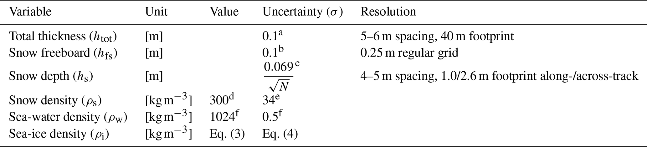
a Pfaffling et al. (2007); Haas et al. (2009). b See Sect. 2.3. c See Sect. 2.4; Jutila et al. (2022). d Warren et al. (1999). e King et al. (2020b). f Wadhams et al. (1992).
2.6 Sea-ice bulk density
Simultaneous measurements of sea-ice thickness, snow depth, and freeboard enable us to calculate sea-ice bulk density using the so-called “freeboard and ice thickness technique” (Timco and Frederking, 1996). Archimedes' principle dictates
where ρ is density for ice, snow, and sea water denoted with subscripts “i”, “s”, and “w”, respectively. The terms can be rearranged to solve for ρi:
By substituting measured total thickness and snow depth for sea-ice thickness () in addition to snow freeboard and snow depth for sea-ice freeboard (), we obtain
To solve Eq. (3), we need to assume values only for the densities of sea water and snow, but their impact on the uncertainty of sea-ice bulk density is small (see Eq. 4 below). Here we took sea-water density and its uncertainty according to Wadhams et al. (1992) as ρw=1024 kg m−3 and kg m−3, respectively. For snow density in April, when measurements were carried out, we chose ρs=300 kg m−3 following Warren et al. (1999) and for the respective uncertainty kg m−3 from King et al. (2020b). These values and the uncertainties of the measured variables are summarised in Table 2. Assuming that the individual uncertainties are uncorrelated, we can derive uncertainty for sea-ice bulk density () using Gaussian error propagation:
Following the uncertainty source analysis of Giles et al. (2007) and using the values summarised in Table 2, the largest contributors to the uncertainty of sea-ice bulk density are, in descending order of magnitude, snow freeboard, snow depth, and total thickness. We disregarded density values with uncertainty exceeding 100 kg m−3 from further analysis.
While the assumption of isostatic equilibrium may not necessarily be valid locally, e.g. close to pressure ridges, it holds true when averaging over a sufficient length scale. We varied the averaging length in 10 m increments and found that the mean bulk densities and the standard deviations for different ice types of the surveys did not change significantly beyond a length scale of about 200 m, if measurements of each ice type were abundant. Here, we computed sea-ice bulk density estimates at two length scales representing the sensor resolution of the CryoSat-2 satellite as well as the typical resolution of gridded sea-ice thickness data. In the first case, we approximated the scale of full-resolution altimeter footprint by the diameter of a circle with the same area as the 300 m×1650 m pulse-Doppler-limited footprint of CryoSat-2 in the synthetic aperture radar (SAR) acquisition mode. The diameter of that circle is equal to approximately 800 m. In the second case, we chose the typical satellite product grid cell size of 25 km. We assumed that the sea-ice and snow layers are in isostatic equilibrium at both scales. We calculated an along-track weighted average using the squares of individual uncertainty values as weights:
where k is the index and N equals the number of values within the length scale to be averaged. The resulting uncertainty was determined with
We also calculated inverse-uncertainty weighted averages for snow depth since its uncertainty varied spatially. For all other variables we calculated an arithmetic mean.
(Alexandrov et al., 2010)Table 3Summary of the 800 m along-track averaged sea-ice bulk density (inverse-uncertainty weighted mean ± 1 standard deviation) according to survey and ice type. The mean values correspond to the red crosses in Fig. 6. The percentage of each sea-ice type encountered on each survey is given in parentheses.
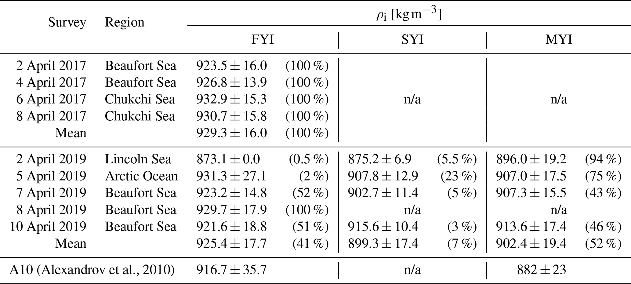
n/a: not applicable
This study included a total of 3410 airborne survey kilometres split approximately equally between the years 2017 and 2019 (Table 1). The abundance of different sea-ice types varied between the years and the individual surveys (see the percentages in Table 3). Surveyed sea ice in 2017 was solely FYI. This was a result of the ice-free conditions in the Beaufort and Chukchi seas in the previous summer, additionally influenced by the collapse of the semipermanent Beaufort high-pressure system, and the subsequent reversal of the Beaufort Gyre in the winter prohibiting typical import of MYI to the region (Babb et al., 2020). In 2019, FYI was encountered primarily in the surveys over the southern Beaufort Sea and the Amundsen Gulf but also embedded within the MYI zone in refrozen leads, constituting 41 % of the calculated density values. The percentage of SYI was generally low, only around 7 %. The largest percentage of SYI was observed in the survey over the Lincoln Sea on 5 April with minor occurrences on other surveys of that year. Similar to SYI, MYI was included only in the surveys in 2019 not only because the imported MYI had returned to the Beaufort Sea within the range of the aircraft but also because the data included surveys over the Lincoln Sea and Arctic Ocean within the Last Ice Area where the oldest and thickest sea ice in the Arctic resides (Moore et al., 2019). Overall, approximately half of the sea ice sampled in 2019 was identified as MYI.
Figure 4 shows the backtracked pathways of the sampled sea ice. ICETrack results from 2017 (panel a) confirmed that all sampled ice was FYI. Indicated sea-ice age was up to approximately 180 d in the Beaufort Sea and up to approximately 150 d in the Chukchi Sea, corresponding to freeze-up in October and November, respectively. In 2019 (panel b), the sampled old ice was indeed up to several years old originating from the Beaufort Gyre. The chosen 25 km backtracking segment length did not resolve any SYI in 2019, pointing to a likely very scarce and localised appearance of SYI.
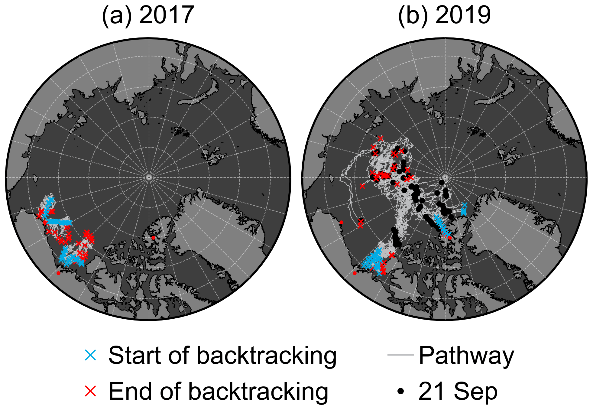
Figure 4Pathways of the sea ice sampled (a) in 2017 and (b) in 2019. Black dots (visible only in panel b) represent the position of the backtracked sea ice on 21 September in the preceding years before sampling, when ice parcels are considered to have survived the summer.
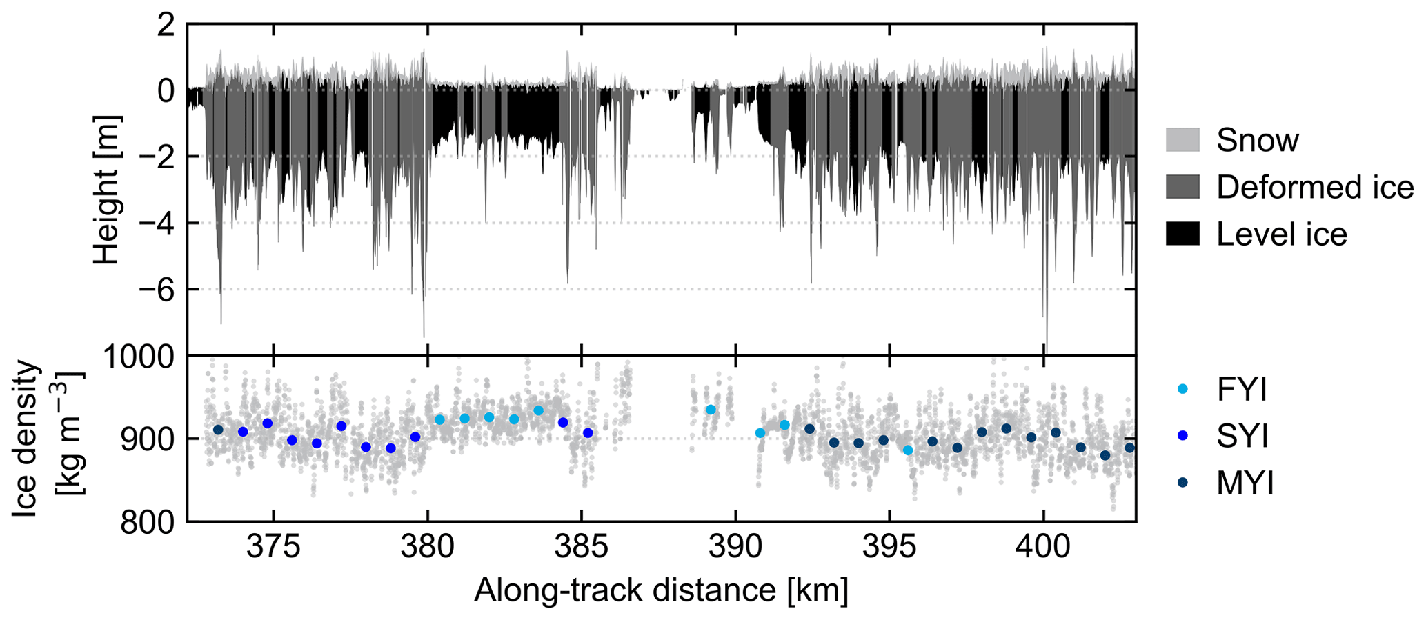
Figure 5Approximately 30 km along-track profile during the survey over the Beaufort Sea on 7 April 2019. The upper panel shows the snow and ice layers, of which the latter is split into deformed and level ice sections, derived from the total thickness, snow freeboard, and snow depth measurements in the native 5–6 m point spacing. The zero height refers to the local sea-surface height. The corresponding calculated sea-ice bulk density values are represented by grey dots in the lower panel together with the 800 m along-track averages that are coded according to the sea-ice type with colour.
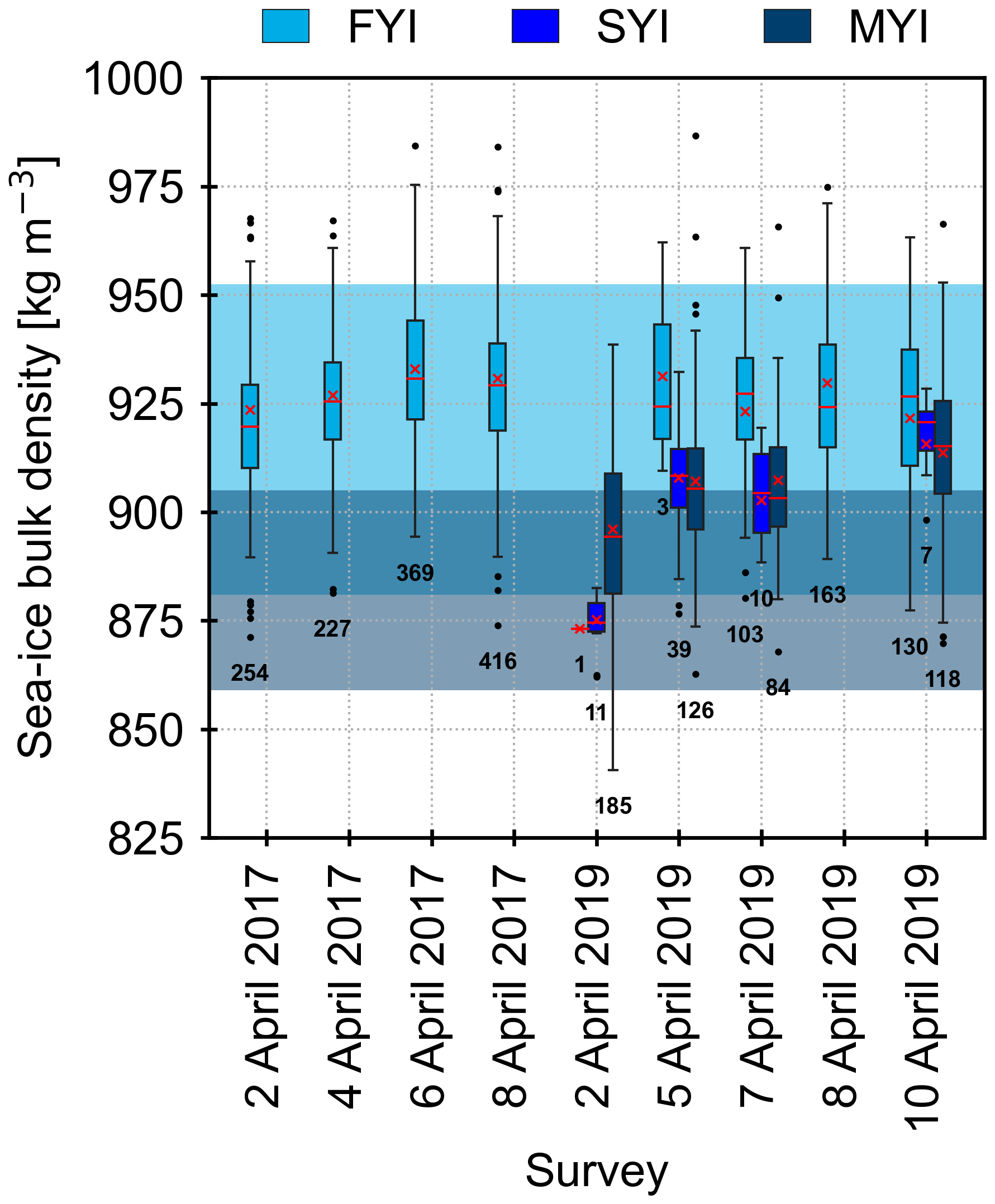
Figure 6Sea-ice bulk density by ice type and survey in the 800 m length scale showing the interquartile range (IQR, Q3–Q1, boxes), the median values (red lines), the inverse-uncertainty weighted mean (red crosses, Table 3), and outliers (beyond 1.5 × IQR, dots). The numbers below the boxes correspond to the number of averaged values contained in each ice type of each individual survey. The shading on the background shows the ± 1 standard deviation range around the A10 mean FYI (light blue) and MYI (dark blue) densities, respectively.
3.1 Sea-ice bulk density
Figure 5 shows an example section of a measured sea-ice profile, roughly 30 km in length along a survey track and including different ice types in the Beaufort Sea in 2019. The bulk densities of FYI, SYI, and MYI, derived using the along-track length scale of 800 m, are stated in Table 3 and shown in Fig. 6. On average, FYI bulk density was higher than the value derived by Alexandrov et al. (2010) (A10), also for individual surveys. FYI bulk density in 2017 was slightly higher than in 2019, and combined they resulted in an average density of 928.5±16.4 kg m−3. SYI and MYI bulk densities differed only a little from each other but were 23–30 kg m−3 lower than FYI bulk density. Similar to FYI, the bulk densities of old ice were in the upper range of or even beyond A10. Figure 7 shows the spatial distribution of the derived sea-ice bulk density when averaged over a typical satellite product grid cell size of 25 km. As expected, lower density values were generally encountered with increasing ice age (Fig. 7e and f). The lowest sea-ice bulk density values were located 50–150 km northwest off the edge of the landfast ice and the coast of Ellesmere Island and Nansen Sound (Fig. 7e). Moreover, there was also noticeable along-track variability of bulk density within a single ice type, even FYI where the highest bulk density values were also observed.
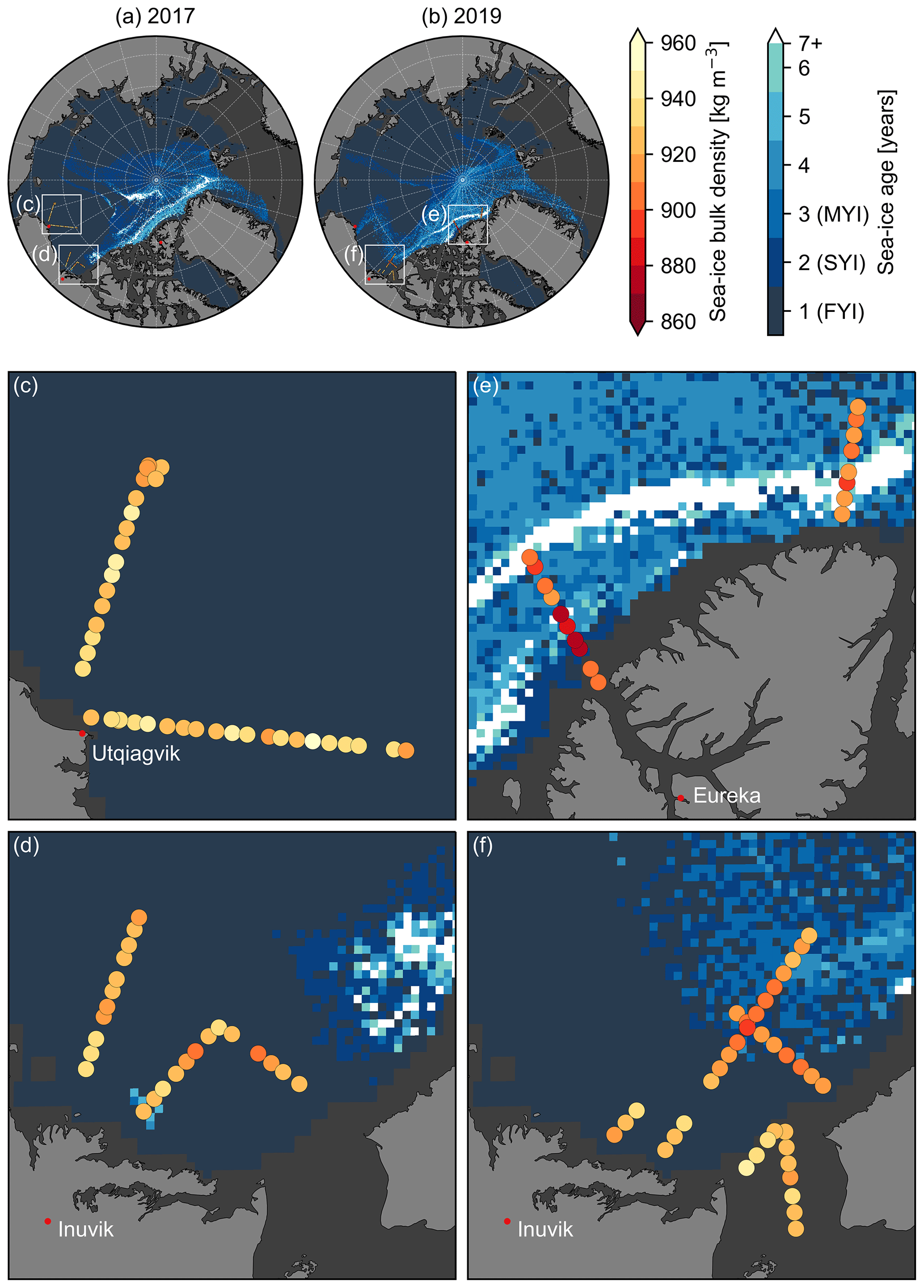
Figure 7Sea-ice bulk density in 25 km along-track segments shown as coloured circles over the weekly NSIDC EASE-Grid Sea Ice Age product (2–8 April; Tschudi et al., 2019) in bluish colours in 2017 (panels a and c–d) and in 2019 (b and e–f). The close-up panels (c)–(f) are 700 km ×700 km in size, and their locations are marked with white squares in the overview panels (a) and (b).
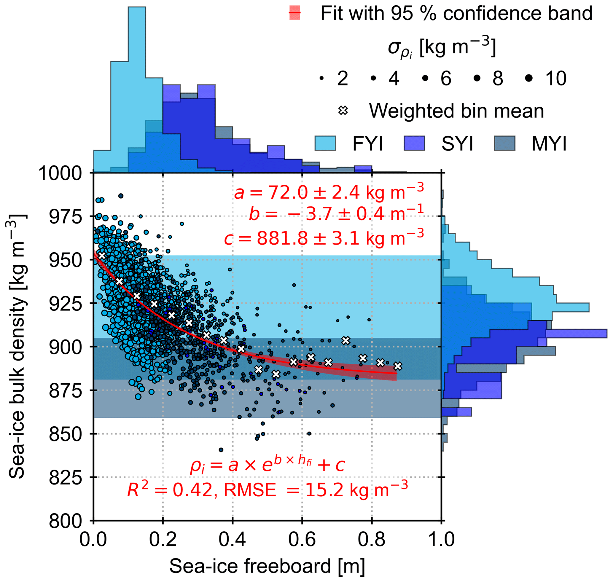
Figure 8Parameterisation of sea-ice bulk density based on sea-ice freeboard. The scatter plot shows all sea-ice bulk density values from 2017 and 2019 in the 800 m length scale (N=2246) against their corresponding sea-ice freeboard values, where the size of the point corresponds to the uncertainty of the density value (). The red line and shading show the non-linear least-squares fit of an exponential function and its 95 % confidence band (Eq. 7). R2 stands for coefficient of determination and RMSE for root-mean-square error of the fitted curve. The crosses are the inverse-uncertainty weighted means using a sea-ice freeboard bin size of 0.05 m. The shading on the background shows the ± 1 standard deviation range around the A10 mean FYI (light blue) and MYI (dark blue) densities. The histograms on the top and on the right show the probability density functions of freeboard and density, respectively, split into different sea-ice types indicated by colour. The respective bin sizes are 0.05 m and 5 kg m−3.
3.2 Parameterisation of sea-ice bulk density
We explored the possibility to parameterise sea-ice bulk density using one of the measured sea-ice parameters. Out of the full parameter space, sea-ice freeboard showed the best correlation with the estimated sea-ice bulk density, (p≪0.001), indicating a significant linear anti-correlation as expected according to Eq. (2) (). However, the dependence on other sea-ice properties and the fact that keels of ridges with high freeboard contain voids filled with sea water introduced non-linearity to this relationship. To avoid underestimating the density values near the lower and upper ends of the observed freeboard range and to increase the goodness of fit, we therefore fitted an exponential function to the full, along-track averaged sea-ice bulk density data set (N=2246, Fig. 8). Least-squares fitting yielded a relationship of
where the parameters with their respective 1 standard deviation errors are kg m−3, kg m−3, and kg m−3. The resulting coefficient of determination (R2) was 0.42 and RMSE was 15.2 kg m−3. A bootstrapping approach with 104 random samples of the size N indicated an RMSE range of 14.8–15.7 kg m−3 with 95 % confidence. The fitted curve showed excellent agreement also with the inverse-uncertainty weighted average densities of the 0.05 m freeboard bins resulting in R2=0.89 and RMSE =6.2 kg m−3. Parameterisation split into different ice types or based on a different parameter, such as sea-ice thickness, surface roughness, or snow depth, resulted in poorer fits and values of R2.
We measure sea-ice bulk density indirectly based on (i) the direct measurements of sea-ice thickness, snow depth, and freeboard and (ii) the isostatic balance between the masses of snow, sea ice, and displaced sea water only assuming the densities of the snow layer and sea water. However, we measure the thickness of the sea-ice layer and not its mass. Instead, we use sea-ice bulk density to relate sea-ice thickness to the displaced mass of sea water inherently by assuming a constant density of the entire sea-ice layer. However, in reality, the material composition of sea ice is not constant throughout the vertical column, which complicates the attribution of bulk sea-ice density values to physical properties such as porosity. Above the waterline, the density is lower than that of pure ice due to air incorporated in the pore spaces. This feature is more pronounced in MYI. Below the waterline, brine and sea water saturate the sea ice and increase the density above the pure ice density. Despite the indirect measurement method, we are able to detect a difference in FYI bulk density between 2017 and 2019 that can be linked to the high sea-ice deformation in 2017. The effect of deformed and unconsolidated sea-ice is often overlooked and needs the attention of the scientific community. Dedicated sea-ice porosity studies and extensive field measurement programmes, such as the recent Multidisciplinary drifting Observatory for the Study of Arctic Climate (MOSAiC), will be able to shed more light on their effect and development.
4.1 Ice-type-averaged sea-ice bulk density
Compared to A10, the average sea-ice bulk density estimates derived in this paper are larger by 11.8 kg m−3 (≈1.3 %) for FYI and by 20.4 kg m−3 (≈2.3 %) for MYI but still within the A10 uncertainties, albeit close to the upper limit. In general, our ice-type-averaged bulk density estimates fall within the range of previous studies (Timco and Frederking, 1996). Reasons for the comparably high estimates are twofold. First, the A10 FYI density is representative only to level, undeformed ice whereas our estimate also includes deformed FYI. Alexandrov et al. (2010) used drill-hole measurements that were carried out in three to five locations, 150–200 m apart around each aircraft landing site on level ice. Sea-water inclusions within deformed and unconsolidated sea ice increase the bulk density. This is a likely reason contributing to the higher FYI bulk density, especially in the 2017 data, given the increased deformation caused by the reversal of the Beaufort Gyre. Second, Alexandrov et al. (2010) calculated the MYI density as a weighted average between the layers above and below the waterline based on values from numerous literature sources but used a density of 550 kg m−3 for the upper layer, which is significantly lower than the majority of the literature indicates (720–910 kg m−3 in Timco and Frederking, 1996; 863–929 kg m−3 in Pustogvar and Kulyakhtin, 2016) and would correspond to an air-volume fraction of up to 40 %. When using the weighted average method in Alexandrov et al. (2010) but the density values from Timco and Frederking (1996) instead, we find a MYI density of 909±28 kg m−3 that is closer to our estimate.
4.2 Uncertainties and limitations of the derived sea-ice bulk density
The effect of the uncertainties in the measured parameters and assumed sea-water and snow density values on the sea-ice bulk density was studied using Gaussian error propagation in Eq. (4). Single point measurements typically resulted in sea-ice bulk density uncertainties of approximately 70 and 35 kg m−3 for FYI and MYI, respectively. Other sources of error arise from the different length scales illustrated in Figs. 3 and 5. We are not able to resolve snow depth fully within the total thickness measurement given the comparably large footprint of the EM-Bird, but we calculate it as an average of the snow depth measurements along a chord of the circular EM-Bird footprint. Due to the cross-track movement of the EM-Bird under the aircraft, the ground locations and the number of the snow depth measurements within the total thickness measurement vary slightly along the survey track but generally remain at 8 to 10 measurements close to the centre line. To ensure representative snow depth estimates, we require at least five valid snow depth measurements for each total thickness measurement, which translates into at least 50 % coverage along the chord. Errors may occur locally, e.g. at cross-track transition from a sea-ice floe to young ice in a newly refrozen lead as in the leftmost measurement points in Fig. 3, but we assume them to occur randomly and not cause systematic bias. However, uncertainties are reduced when averaged along-track over a length scale. Using the 800 m length scale, the resulting sea-ice bulk density uncertainty is generally less than 10 kg m−3 (Eq. 6) but remain the highest for thin ice and low sea-ice freeboard where the relative uncertainties of the input parameters are the largest (see the size of the scatter points in Fig. 8). In turn, averaging over a length scale simplifies the natural variability of sea ice. Figure 5 shows how a single 25 km satellite grid cell can already contain several sea-ice types: level, deformed, FYI, SYI, and MYI. However, assigning the sea-ice types is limited by the spatial (12.5 km) and temporal (weekly) resolution of the NSIDC sea-ice age product, which we try to compensate for with the additional thickness-based conditions (see Sect. 2.5.2). In addition and similar to Alexandrov et al. (2010), the data are seasonally and regionally limited. Our measurements are confined to the western Arctic in early April, and therefore, more measurements across the Arctic and the seasons are needed to evaluate the spatial and temporal variability of sea-ice bulk density.
4.3 Impact on sea-ice thickness retrievals
Assuming all the other parameters for the conversion of freeboard to thickness remain the same, the average sea-ice bulk density estimates derived in this paper would result in 12.4 % and 16.7 % larger sea-ice thickness values for FYI and MYI, respectively, in comparison to A10. The effect is larger for thicker ice, for which snow depth plays a proportionally less important role. Therefore, improving in particular the MYI bulk density is important to derive accurate time series of sea-ice thickness and volume, as in the past, thicker MYI represented a larger fraction of the Arctic sea-ice cover. Kwok and Cunningham (2015) recognised the possibility of varying MYI density between the recent younger MYI and older MYI of the previous decades and discussed the impact of MYI density on sea-ice thickness and volume. Moreover, a potentially increasing degree of deformation may lead to a bias in the time series, as satellites underestimate sea-ice draft of deformed ice as shown by Belter et al. (2020) and further discussed by Khvorostovsky et al. (2020). Deformed and unconsolidated sea ice has an increased bulk density due to sea-water inclusions, and thus, using a typical density of consolidated level sea ice for deriving sea-ice thickness from satellite data will eventually lead to an underestimation. Given the thinner and younger sea-ice cover together with observed increase in sea-ice drift speed and deformation (Rampal et al., 2009; Spreen et al., 2011), there is a likely premise for systematic underestimation by current parameterisations of sea-ice density in regions where and at times when sea ice is deformed. A full impact assessment of the sea-ice bulk density parameterisation on decadal sea-ice thickness data record is a logical next step but beyond the scope of this paper.
4.4 Outlook
To represent sea-ice bulk density range as a functional relationship to a parameter observable from space rather than fixed values based on sea-ice type classification, we parameterised sea-ice bulk density using sea-ice freeboard and obtained a significant correlation. Opting for an exponential function instead of linear was beneficial for ensuring a better fit, capturing the high bulk density values at low freeboard values and avoiding linear decrease to possibly unrepresentative and unphysical values at high freeboards. Parameterisation in Eq. (7) sets the limits of bulk density to 953.8 kg m−3 at zero sea-ice freeboard and approaching 881.8 kg m−3 at high freeboards.
Figure 9 shows the parameterisation in Eq. (7) applied to the AWI Level-3 Collocated CryoSat-2 Sea Ice Product (Hendricks and Ricker, 2020) from the winter 2018/2019, converting the monthly gridded sea-ice freeboard to sea-ice density. The resulting sea-ice density distribution had a smoother transition between ice types compared to the current ice-type-dependent density classification of the retrieval algorithm. Difference between the density parameterised with Eq. (7) and A10 was positive overall during the winter except in the central Arctic Ocean and locally in the Fram and Bering straits in spring. The density difference was the largest on MYI in proximity to FYI but decreased toward spring.

Figure 9Sea-ice density parameterisation applied to the monthly gridded AWI CryoSat-2 Sea Ice Product (Hendricks and Ricker, 2020) for the winter 2018/2019. The rows show sea-ice freeboard, sea-ice density derived using Eq. (7) (J21), sea-ice density currently used in the product (A10), and the difference between the two (J21 − A10). The columns from left to right show monthly means from October 2018 to April 2019.
Only less than 3 % of the airborne data set has a sea-ice freeboard value larger than 0.5 m, with considerable spread in bulk density values and thus introducing uncertainty to the parameterisation at high freeboard values. Constraining the parameterisation at high freeboards would require more data in deformed and multi-year sea-ice environments. However, that needs to coincide with a sufficient number of open leads to ensure accurate conversion of surface elevations to freeboard from the ALS. With the limitations of the current method, it is also not feasible to investigate cases of negative sea-ice freeboard due to the possible presence of liquid water and altered dielectric properties affecting the retrieval of snow depth.
Our parameterisation improves upon the previous formulations of sea-ice density given the significantly larger number of data points, larger areal coverage, the variety of ice types including deformed sea ice, and the choice of predictor variable it is based on. Kovacs (1997) based his analysis on 17 FYI and 4 MYI sea-ice cores from the Beaufort Sea and derived a floe-thickness-based non-linear parameterisation of . Ackley et al. (1976) used drill-hole measurements from 400 m of profile lines in the Beaufort Sea to derive , where is effective freeboard and the overbar denotes average density on the floe. The parameters needed for those formulations cannot be directly observed from space, or in the case of effective freeboard not even with a single in situ measurement, which makes them difficult to apply. Demonstrated in Fig. 9, our freeboard-based parameterisation has potential for future applications in satellite altimetry. While we acknowledge that, due to the variability in snow mass and sea-ice thickness, our parameterisation may not be applicable on sub-kilometre scales as reflected by the scatter in Fig. 8, we think that a sea-ice density parameterisation is a significant improvement upon a single value or fixed values based on ice type. In this paper, we decided to adopt a single-predictor parameterisation for the sake of simplicity. However, for future studies it could be worthwhile, for example, to apply machine learning algorithms to the full parameter space to discover possible multi-variable relationships. Given the effect of sea-ice deformation on bulk density, including sea-ice surface roughness, a multi-variable approach could explain more of the variability.
The unique, collocated, multi-sensor measurements of the Arctic sea ice from the AWI IceBird campaigns allow us not only to observe sea-ice thickness, freeboard, and snow depth in high-resolution on regional scales, but also for the first time to estimate sea-ice bulk densities of different ice types from airborne measurements. Despite measuring the sea-ice bulk density indirectly by deriving it from other measurements, we are able to capture the effects of deformed ice on FYI bulk density. In the current Arctic, the average late-winter FYI and MYI bulk densities are higher than and do not differ as much as earlier studies suggested, partly due to including deformed ice in the analysis. Alexandrov et al. (2010) derived a difference of 34.7 kg m−3, whereas our measurements show only 26.1 kg m−3, providing yet one more indication and consequence that the Arctic sea-ice cover is getting younger. Satellite altimetry sea-ice thickness retrieval algorithms need to adapt to these changes in order to capture the sea-ice thickness and volume accurately and to account for changes over the satellite radar altimetry record spanning almost 3 decades. Taking advantage of the abundant measurements collected over different sea-ice types during two late-winter airborne campaigns, we are able to provide a parameterisation of sea-ice bulk density using sea-ice freeboard. The single-variable exponential function presented here yields a smaller RMSE than the uncertainty of density values fixed by sea-ice type currently in use to a large extent. With potential applications in sea-ice thickness retrieval from satellite radar altimetry, a density parameterisation alone does not completely solve the uncertainty problem in the freeboard-to-thickness conversion. Together with improved knowledge of snow loading, they provide a path to decrease the uncertainty in observing sea-ice thickness and volume where the recent (CryoSat-2/ICESat-2 orbit resonance) and future (CRISTAL mission) advances in dual altimetry will play a key role. In situ and airborne multi-sensor observations of various sea-ice parameters across the seasons will remain important to validate new approaches.
The Python package pySnowRadar (King et al., 2020a) used in this study to retrieve snow depth from radar data is available at https://doi.org/10.5281/ZENODO.4071801. Collocated sea-ice parameter data products, including measured total thickness, snow freeboard, snow depth, and surface temperature and derived parameters such as sea-ice thickness, sea-ice freeboard, and sea-ice bulk density, are available on PANGAEA (https://doi.org/10.1594/PANGAEA.933883, Jutila et al., 2021a, and https://doi.org/10.1594/PANGAEA.933912, Jutila et al., 2021b). Release of lower-processing-level data is under preparation. Total thickness measurements during the PAMARCMIP2017 campaign are already available at https://doi.org/10.1594/PANGAEA.924848 (Hendricks et al., 2020). The EASE-Grid Sea Ice Age, Version 4, is available from the NASA National Snow and Ice Data Center Distributed Active Archive Center: https://doi.org/10.5067/UTAV7490FEPB (Tschudi et al., 2019). The Canadian Ice Service Arctic Regional Sea Ice Charts in SIGRID-3 Format, Version 1, are available from the NSIDC: National Snow and Ice Data Center: https://doi.org/10.7265/N51V5BW9 (Canadian Ice Service, 2009). The AWI Level-3 Collocated CryoSat-2 Sea Ice Product is available here: ftp://ftp.awi.de/sea_ice/product/cryosat2/v2p3/ (Hendricks and Ricker, 2020).
AJ carried out the analysis with support from SH and RR and prepared the manuscript with input from SH, RR, LvA, TK, and CH. AJ, SH, and RR collected the data. SH applied the density parameterisation to the CryoSat-2 data and produced Fig. 9. LvA processed the EM-Bird data to identify level and deformed ice. TK conducted the backward tracking of sea ice with ICETrack.
At least one of the (co-)authors is a member of the editorial board of The Cryosphere. The peer-review process was guided by an independent editor, and the authors also have no other competing interests to declare.
Publisher's note: Copernicus Publications remains neutral with regard to jurisdictional claims in published maps and institutional affiliations.
The authors thank the crews of Polar 5 and 6, Kenn Borek Air, AWI technicians and logistics, Environment and Climate Change Canada (ECCC), and Canadian Forces Station (CFS) Alert, who helped at various stages of the data collection. Veit Helm is acknowledged for post-processing the surface temperature data.
The authors thank Dmitry Divine and the one anonymous referee for their valuable and constructive comments and suggestions during the review process. Thanks to editor Michel Tsamados and the team at The Cryosphere for their support and processing of our paper.
The article processing charges for this open-access publication were covered by the Alfred Wegener Institute, Helmholtz Centre for Polar and Marine Research (AWI).
This paper was edited by Michel Tsamados and reviewed by Dmitry Divine and one anonymous referee.
Ackley, S. F., Hibler, W. D., Kugzruk, F. K., Kovacs, A., and Weeks, W. F.: Thickness and roughness variations of Arctic multiyear sea ice, Cold Regions Research and Engineering Laboratory, Tech. Rep. 76-18, 1976. a, b
Alexandrov, V., Sandven, S., Wahlin, J., and Johannessen, O. M.: The relation between sea ice thickness and freeboard in the Arctic, The Cryosphere, 4, 373–380, https://doi.org/10.5194/tc-4-373-2010, 2010. a, b, c, d, e, f, g, h, i
Alfred-Wegener-Institut Helmholtz-Zentrum für Polar- und Meeresforschung: Polar aircraft Polar5 and Polar6 operated by the Alfred Wegener Institute, Journal of large-scale research facilities JLSRF, 2, A87, https://doi.org/10.17815/jlsrf-2-153, 2016. a
Andersen, O. B., Piccioni, G., Stenseng, L., and Knudsen, P.: The DTU15 MSS (Mean Sea Surface) and DTU15LAT (Lowest Astronomical Tide) reference surface, available at: https://ftp.space.dtu.dk/pub/DTU15/DOCUMENTS/MSS/DTU15MSS+LAT.pdf (last access: 9 February 2021), 2016. a
AWI IceBird program: https://www.awi.de/en/science/climate-sciences/sea-ice-physics/projects/ice-bird.html (last access: 10 May 2021), 2020. a
Babb, D. G., Landy, J. C., Lukovich, J. V., Haas, C., Hendricks, S., Barber, D. G., and Galley, R. J.: The 2017 Reversal of the Beaufort Gyre: Can Dynamic Thickening of a Seasonal Ice Cover During a Reversal Limit Summer Ice Melt in the Beaufort Sea?, J. Geophys. Res.-Oceans, 125, e2020JC016796, https://doi.org/10.1029/2020JC016796, 2020. a
Barber, D. G., Reddan, S. P., and LeDrew, E. F.: Statistical characterization of the geophysical and electrical properties of snow on landfast first-year sea ice, J. Geophys. Res., 100, 2673–2686, https://doi.org/10.1029/94JC02200, 1995. a
Belter, H. J., Krumpen, T., Hendricks, S., Hoelemann, J., Janout, M. A., Ricker, R., and Haas, C.: Satellite-based sea ice thickness changes in the Laptev Sea from 2002 to 2017: comparison to mooring observations, The Cryosphere, 14, 2189–2203, https://doi.org/10.5194/tc-14-2189-2020, 2020. a
Canadian Ice Service: Canadian Ice Service Arctic Regional Sea Ice Charts in SIGRID-3 Format, Version 1, NSIDC: National Snow and Ice Data Center [data set], Boulder, Colorado, USA, https://doi.org/10.7265/N51V5BW9, 2009. a, b
Comiso, J. C.: Large Decadal Decline of the Arctic Multiyear Ice Cover, J. Climate, 25, 1176–1193, https://doi.org/10.1175/JCLI-D-11-00113.1, 2012. a
Duchossois, G., Strobl, P., Toumazou, V., Antunes, S., Bartsch, A., Diehl, T., Dinessen, F., Eriksson, P., Garric, G., Houssais, M.-N., Jindrova, M., Muñoz-Sabater, J., Nagler, T., and Nordbeck, O.: User Requirements for a Copernicus Polar Mission – Phase 1 Report, Publications Office of the European Union, Luxembourg, https://doi.org/10.2760/22832, 2018. a
Ezraty, R., Girard-Ardhuin, F., Piollé, J.-F., Kaleschke, L., and Heygster, G.: Arctic & Antarctic sea ice concentration and Arctic sea ice drift estimated from special sensor microwave data – User's manual, Laboratoire d'Océanographie Spatiale Département d'Océanographie Physique et Spatiale IFREMER, Brest, France and Institute of Environmental Physics University of Bremen, Germany, available at: ftp://ftp.ifremer.fr/ifremer/cersat/products/gridded/psi-drift/documentation/ssmi.pdf (last access: 21 January 2021), 2007. a
Giles, K., Laxon, S., Wingham, D., Wallis, D., Krabill, W., Leuschen, C., McAdoo, D., Manizade, S., and Raney, R.: Combined airborne laser and radar altimeter measurements over the Fram Strait in May 2002, Remote Sens. Environ., 111, 182–194, https://doi.org/10.1016/j.rse.2007.02.037, 2007. a, b
Haas, C., Gerland, S., Eicken, H., and Miller, H.: Comparison of sea‐ice thickness measurements under summer and winter conditions in the Arctic using a small electromagnetic induction device, Geophysics, 62, 749–757, https://doi.org/10.1190/1.1444184, 1997. a
Haas, C., Lobach, J., Hendricks, S., Rabenstein, L., and Pfaffling, A.: Helicopter-borne measurements of sea ice thickness, using a small and lightweight, digital EM system, J. Appl. Geophys., 67, 234–241, https://doi.org/10.1016/j.jappgeo.2008.05.005, 2009. a, b, c, d, e
Haas, C., Hendricks, S., Eicken, H., and Herber, A.: Synoptic airborne thickness surveys reveal state of Arctic sea ice cover, Geophys. Res. Lett., 37, L09501, https://doi.org/10.1029/2010GL042652, 2010. a
Haas, C., Langhorne, P. J., Rack, W., Leonard, G. H., Brett, G. M., Price, D., Beckers, J. F., and Gough, A. J.: Airborne mapping of the sub-ice platelet layer under fast ice in McMurdo Sound, Antarctica, The Cryosphere, 15, 247–264, https://doi.org/10.5194/tc-15-247-2021, 2021. a
Hendricks, S. and Ricker, R.: Product User Guide & Algorithm Specification AWI CryoSat-2 Sea Ice Thickness (version 2.3), Alfred Wegener Institute Helmholtz Centre for Polar and Marine Research, https://hdl.handle.net/10013/epic.ecd56b5d-3e7d-4a65-9019-588b1c3b0d26 (last access: 9 April 2021), 2020. a, b, c
Hendricks, S., Ricker, R., Haas, C., and Herber, A.: Airborne sea ice plus snow thickness during the PAMARCMIP 2017 aircraft campaign in the Arctic Ocean, PANGAEA [data set], https://doi.org/10.1594/PANGAEA.924848, 2020. a
Herber, A. B., Haas, C., Stone, R. S., Bottenheim, J. W., Liu, P., Li, S.-M., Staebler, R. M., Strapp, J. W., and Dethloff, K.: Regular airborne surveys of Arctic sea ice and atmosphere, Eos, Transactions American Geophysical Union, 93, 41–42, https://doi.org/10.1029/2012EO040001, 2012. a
Hunke, E. C., Notz, D., Turner, A. K., and Vancoppenolle, M.: The multiphase physics of sea ice: a review for model developers, The Cryosphere, 5, 989–1009, https://doi.org/10.5194/tc-5-989-2011, 2011. a
Jutila, A., Hendricks, S., Ricker, R., von Albedyll, L., and Haas, C.: Airborne sea ice parameters during the PAMARCMIP2017 campaign in the Arctic Ocean, version 1, PANGAEA [data set], https://doi.org/10.1594/PANGAEA.933883, 2021a. a
Jutila, A., Hendricks, S., Ricker, R., von Albedyll, L., and Haas, C.: Airborne sea ice parameters during the IceBird Winter 2019 campaign in the Arctic Ocean, version 1, PANGAEA [data set], https://doi.org/10.1594/PANGAEA.933912, 2021b. a
Jutila, A., King, J., Paden, J., Ricker, R., Hendricks, S., Polashenski, C., Helm, V., Binder, T., and Haas, C.: High-Resolution Snow Depth on Arctic Sea Ice From Low-Altitude Airborne Microwave Radar Data, IEEE T. Geosci. Remote, 60, 4300716, https://doi.org/10.1109/TGRS.2021.3063756, 2022. a, b, c, d, e, f
Kern, M., Cullen, R., Berruti, B., Bouffard, J., Casal, T., Drinkwater, M. R., Gabriele, A., Lecuyot, A., Ludwig, M., Midthassel, R., Navas Traver, I., Parrinello, T., Ressler, G., Andersson, E., Martin-Puig, C., Andersen, O., Bartsch, A., Farrell, S., Fleury, S., Gascoin, S., Guillot, A., Humbert, A., Rinne, E., Shepherd, A., van den Broeke, M. R., and Yackel, J.: The Copernicus Polar Ice and Snow Topography Altimeter (CRISTAL) high-priority candidate mission, The Cryosphere, 14, 2235–2251, https://doi.org/10.5194/tc-14-2235-2020, 2020. a
Khvorostovsky, K., Hendricks, S., and Rinne, E.: Surface Properties Linked to Retrieval Uncertainty of Satellite Sea-Ice Thickness with Upward-Looking Sonar Measurements, Remote Sens., 12, 3094, https://doi.org/10.3390/rs12183094, 2020. a
King, J., Brady, M., and Newman, T.: kingjml/pySnowRadar: IEEE TGRS Submission, Zenodo [code], https://doi.org/10.5281/ZENODO.4071801, 2020a. a
King, J., Howell, S., Brady, M., Toose, P., Derksen, C., Haas, C., and Beckers, J.: Local-scale variability of snow density on Arctic sea ice, The Cryosphere, 14, 4323–4339, https://doi.org/10.5194/tc-14-4323-2020, 2020b. a, b
Kovacs, A.: Estimating the full-scale flexural and compressive strength of first-year sea ice, J. Geophys. Res.-Oceans, 102, 8681–8689, https://doi.org/10.1029/96JC02738, 1997. a, b
Kovacs, A. and Morey, R. M.: Sounding sea ice thickness using a portable electromagnetic induction instrument, Geophysics, 56, 1992–1998, https://doi.org/10.1190/1.1443011, 1991. a
Krumpen, T.: AWI ICETrack: Antarctic and Arctic Sea Ice Monitoring and Tracking Tool, Vers. 1.3, Alfred Wegener Institute Helmholtz Centre for Polar and Marine Research, https://hdl.handle.net/10013/epic.9ee550b6-5966-4db6-a042-f4256810ec3f (last access: 21 January 2021), 2018. a
Krumpen, T., Belter, H. J., Boetius, A., Damm, E., Haas, C., Hendricks, S., Nicolaus, M., Nöthig, E. M., Paul, S., Peeken, I., Ricker, R., and Stein, R.: Arctic warming interrupts the Transpolar Drift and affects long-range transport of sea ice and ice-rafted matter, Sci. Rep.-UK, 9, 5459, https://doi.org/10.1038/s41598-019-41456-y, 2019. a
Krumpen, T., Birrien, F., Kauker, F., Rackow, T., von Albedyll, L., Angelopoulos, M., Belter, H. J., Bessonov, V., Damm, E., Dethloff, K., Haapala, J., Haas, C., Harris, C., Hendricks, S., Hoelemann, J., Hoppmann, M., Kaleschke, L., Karcher, M., Kolabutin, N., Lei, R., Lenz, J., Morgenstern, A., Nicolaus, M., Nixdorf, U., Petrovsky, T., Rabe, B., Rabenstein, L., Rex, M., Ricker, R., Rohde, J., Shimanchuk, E., Singha, S., Smolyanitsky, V., Sokolov, V., Stanton, T., Timofeeva, A., Tsamados, M., and Watkins, D.: The MOSAiC ice floe: sediment-laden survivor from the Siberian shelf, The Cryosphere, 14, 2173–2187, https://doi.org/10.5194/tc-14-2173-2020, 2020. a
Kurtz, N. T. and Farrell, S. L.: Large-scale surveys of snow depth on Arctic sea ice from Operation IceBridge, Geophys. Res. Lett., 38, L20505, https://doi.org/10.1029/2011GL049216, 2011. a, b, c
Kurtz, N. T., Farrell, S. L., Studinger, M., Galin, N., Harbeck, J. P., Lindsay, R., Onana, V. D., Panzer, B., and Sonntag, J. G.: Sea ice thickness, freeboard, and snow depth products from Operation IceBridge airborne data, The Cryosphere, 7, 1035–1056, https://doi.org/10.5194/tc-7-1035-2013, 2013. a, b
Kwok, R.: Satellite remote sensing of sea-ice thickness and kinematics: a review, J. Glaciol., 56, 1129–1140, https://doi.org/10.3189/002214311796406167, 2010. a
Kwok, R. and Cunningham, G. F.: Variability of Arctic sea ice thickness and volume from CryoSat-2, Philos. T. Roy. Soc. A, 373, 20140157, https://doi.org/10.1098/rsta.2014.0157, 2015. a
Landy, J. C., Petty, A. A., Tsamados, M., and Stroeve, J. C.: Sea Ice Roughness Overlooked as a Key Source of Uncertainty in CryoSat‐2 Ice Freeboard Retrievals, J. Geophys. Res.-Oceans, 125, e2019JC015820, https://doi.org/10.1029/2019JC015820, 2020. a
Lavergne, T., Eastwood, S., Teffah, Z., Schyberg, H., and Breivik, L.-A.: Sea ice motion from low-resolution satellite sensors: An alternative method and its validation in the Arctic, J. Geophys. Res., 115, C10032, https://doi.org/10.1029/2009JC005958, 2010. a
MacGregor, J. A., Boisvert, L. N., Medley, B., Petty, A. A., Harbeck, J. P., Bell, R. E., Blair, J. B., Blanchard‐Wrigglesworth, E., Buckley, E. M., Christoffersen, M. S., Cochran, J. R., Csathó, B. M., De Marco, E. L., Dominguez, R. T., Fahnestock, M. A., Farrell, S. L., Gogineni, S. P., Greenbaum, J. S., Hansen, C. M., Hofton, M. A., Holt, J. W., Jezek, K. C., Koenig, L. S., Kurtz, N. T., Kwok, R., Larsen, C. F., Leuschen, C. J., Locke, C. D., Manizade, S. S., Martin, S., Neumann, T. A., Nowicki, S. M., Paden, J. D., Richter‐Menge, J. A., Rignot, E. J., Rodríguez‐Morales, F., Siegfried, M. R., Smith, B. E., Sonntag, J. G., Studinger, M., Tinto, K. J., Truffer, M., Wagner, T. P., Woods, J. E., Young, D. A., and Yungel, J. K.: The scientific legacy of NASA's Operation IceBridge, Rev. Geophys., 59, e2020RG000712, https://doi.org/10.1029/2020RG000712, 2021. a
Maslanik, J., Stroeve, J., Fowler, C., and Emery, W.: Distribution and trends in Arctic sea ice age through spring 2011, Geophys. Res. Lett., 38, L13502, https://doi.org/10.1029/2011GL047735, 2011. a
Meier, W. N., Hovelsrud, G. K., van Oort, B. E., Key, J. R., Kovacs, K. M., Michel, C., Haas, C., Granskog, M. A., Gerland, S., Perovich, D. K., Makshtas, A., and Reist, J. D.: Arctic sea ice in transformation: A review of recent observed changes and impacts on biology and human activity, Rev. Geophys., 52, 185–217, https://doi.org/10.1002/2013RG000431, 2014. a
Moore, G. W. K., Schweiger, A., Zhang, J., and Steele, M.: Spatiotemporal Variability of Sea Ice in the Arctic's Last Ice Area, Geophys. Res. Lett., 46, 11237–11243, https://doi.org/10.1029/2019GL083722, 2019. a
Petrich, C. and Eicken, H.: Overview of sea ice growth and properties, in: Sea Ice, edited by: Thomas, D. N., John Wiley & Sons, Ltd, Chichester, UK, third edn., chap. 1, 1–41, https://doi.org/10.1002/9781118778371.ch1, 2017. a
Pfaffling, A., Haas, C., and Reid, J. E.: Direct helicopter EM – Sea-ice thickness inversion assessed with synthetic and field data, Geophysics, 72, F127–F137, https://doi.org/10.1190/1.2732551, 2007. a, b
Pounder, E. R.: The Physics of Ice, Pergamon Press, Oxford, first edn., https://doi.org/10.1016/C2013-0-08278-3, 1965. a
Pustogvar, A. and Kulyakhtin, A.: Sea ice density measurements. Methods and uncertainties, Cold Reg. Sci. Technol., 131, 46–52, https://doi.org/10.1016/j.coldregions.2016.09.001, 2016. a, b
Quartly, G. D., Rinne, E., Passaro, M., Andersen, O. B., Dinardo, S., Fleury, S., Guillot, A., Hendricks, S., Kurekin, A. A., Müller, F. L., Ricker, R., Skourup, H., and Tsamados, M.: Retrieving Sea Level and Freeboard in the Arctic: A Review of Current Radar Altimetry Methodologies and Future Perspectives, Remote Sens., 11, 881, https://doi.org/10.3390/rs11070881, 2019. a
Rabenstein, L., Hendricks, S., Martin, T., Pfaffhuber, A., and Haas, C.: Thickness and surface-properties of different sea-ice regimes within the Arctic Trans Polar Drift: Data from summers 2001, 2004 and 2007, J. Geophys. Res., 115, C12059, https://doi.org/10.1029/2009JC005846, 2010. a, b
Rampal, P., Weiss, J., and Marsan, D.: Positive trend in the mean speed and deformation rate of Arctic sea ice, 1979–2007, J. Geophys. Res., 114, C05013, https://doi.org/10.1029/2008JC005066, 2009. a
Ricker, R., Hendricks, S., Helm, V., Skourup, H., and Davidson, M.: Sensitivity of CryoSat-2 Arctic sea-ice freeboard and thickness on radar-waveform interpretation, The Cryosphere, 8, 1607–1622, https://doi.org/10.5194/tc-8-1607-2014, 2014. a
Ricker, R., Hendricks, S., and Beckers, J. F.: The Impact of Geophysical Corrections on Sea-Ice Freeboard Retrieved from Satellite Altimetry, Remote Sens., 8, 317, https://doi.org/10.3390/rs8040317, 2016. a
Rösel, A., Farrell, S. L., Nandan, V., Richter-Menge, J., Spreen, G., Divine, D. V., Steer, A., Gallet, J.-C., and Gerland, S.: Implications of surface flooding on airborne estimates of snow depth on sea ice, The Cryosphere, 15, 2819–2833, https://doi.org/10.5194/tc-15-2819-2021, 2021. a, b
Sallila, H., Farrell, S. L., McCurry, J., and Rinne, E.: Assessment of contemporary satellite sea ice thickness products for Arctic sea ice, The Cryosphere, 13, 1187–1213, https://doi.org/10.5194/tc-13-1187-2019, 2019. a, b
SIMIP Community: Arctic Sea Ice in CMIP6, Geophys. Res. Lett., 47, e2019GL086749, https://doi.org/10.1029/2019GL086749, 2020. a
Spreen, G., Kwok, R., and Menemenlis, D.: Trends in Arctic sea ice drift and role of wind forcing: 1992–2009, Geophys. Res. Lett., 38, L19501, https://doi.org/10.1029/2011GL048970, 2011. a
Stroeve, J. and Notz, D.: Changing state of Arctic sea ice across all seasons, Environ. Res. Lett., 13, 103001, https://doi.org/10.1088/1748-9326/aade56, 2018. a, b, c
Timco, G. W. and Frederking, R. M.: A review of sea ice density, Cold Reg. Sci. Technol., 24, 1–6, https://doi.org/10.1016/0165-232X(95)00007-X, 1996. a, b, c, d, e, f, g, h
Timco, G. W. and Weeks, W. F.: A review of the engineering properties of sea ice, Cold Reg. Sci. Technol., 60, 107–129, https://doi.org/10.1016/j.coldregions.2009.10.003, 2010. a
Tschudi, M., Meier, W. N., Stewart, J. S., Fowler, C., and Maslanik, J.: EASE-Grid Sea Ice Age, Version 4, NASA National Snow and Ice Data Center Distributed Active Archive Center [data set], Boulder, Colorado, USA, https://doi.org/10.5067/UTAV7490FEPB, 2019. a, b, c
Wadhams, P., Tucker, W. B., Krabill, W. B., Swift, R. N., Comiso, J. C., and Davis, N. R.: Relationship between sea ice freeboard and draft in the Arctic Basin, and implications for ice thickness monitoring, J. Geophys. Res., 97, 20325–20334, https://doi.org/10.1029/92JC02014, 1992. a, b
Warren, S. G., Rigor, I. G., Untersteiner, N., Radionov, V. F., Bryazgin, N. N., Aleksandrov, Y. I., and Colony, R.: Snow Depth on Arctic Sea Ice, J. Climate, 12, 1814–1829, https://doi.org/10.1175/1520-0442(1999)012<1814:SDOASI>2.0.CO;2, 1999. a, b, c
Yan, J.-B., Gogineni, S., Rodriguez-Morales, F., Gomez-Garcia, D., Paden, J., Li, J., Leuschen, C. J., Braaten, D. A., Richter-Menge, J. A., Farrell, S. L., Brozena, J., and Hale, R. D.: Airborne Measurements of Snow Thickness: Using ultrawide-band frequency-modulated-continuous-wave radars, IEEE Geosci. Remote Sens. Mag., 5, 57–76, https://doi.org/10.1109/MGRS.2017.2663325, 2017. a
Zhou, L., Stroeve, J., Xu, S., Petty, A., Tilling, R., Winstrup, M., Rostosky, P., Lawrence, I. R., Liston, G. E., Ridout, A., Tsamados, M., and Nandan, V.: Inter-comparison of snow depth over Arctic sea ice from reanalysis reconstructions and satellite retrieval, The Cryosphere, 15, 345–367, https://doi.org/10.5194/tc-15-345-2021, 2021. a
Zygmuntowska, M., Rampal, P., Ivanova, N., and Smedsrud, L. H.: Uncertainties in Arctic sea ice thickness and volume: new estimates and implications for trends, The Cryosphere, 8, 705–720, https://doi.org/10.5194/tc-8-705-2014, 2014. a