Land–atmosphere interactions in sub-polar and alpine climates in the CORDEX flagship pilot study Land Use and Climate Across Scales (LUCAS) models – Part 1: Evaluation of the snow-albedo effect

Seasonal snow cover plays a major role in the climate system of the Northern Hemisphere via its effect on land surface albedo and fluxes. In climate models the parameterization of interactions between snow and atmosphere remains a source of uncertainty and biases in the representation of local and global climate. Here, we evaluate the ability of an ensemble of regional climate models (RCMs) coupled with different land surface models to simulate snow–atmosphere interactions over Europe in winter and spring. We use a previously defined index, the snow-albedo sensitivity index (SASI), to quantify the radiative forcing associated with snow cover anomalies. By comparing RCM-derived SASI values with SASI calculated from reanalyses and satellite retrievals, we show that an accurate simulation of snow cover is essential for correctly reproducing the observed forcing over middle and high latitudes in Europe. The choice of parameterizations, and primarily the choice of the land surface model, strongly influences the representation of SASI as it affects the ability of climate models to simulate snow cover accurately. The degree of agreement between the datasets differs between the accumulation and ablation periods, with the latter one presenting the greatest challenge for the RCMs. Given the dominant role of land surface processes in the simulation of snow cover during the ablation period, the results suggest that, during this time period, the choice of the land surface model is more critical for the representation of SASI than the atmospheric model.

1 Introduction

Snow is an important part of the climate system, regulating the temperature of the Earth's surface via its effect on surface albedo and surface fluxes. In mid- and high-latitude regions, snow is the main interface through which land interacts with the atmosphere during the cold season, and the importance of snow–atmosphere interactions in modulating the energy budget at high latitudes during winter has been demonstrated (Diro and Sushama, 2018; Henderson et al., 2018; Xu and Dirmeyer, 2013a). Snow cover extent and depth can modify both surface energy and moisture budgets, triggering complex feedback mechanisms that impact both local and remote climates (Diro and Sushama, 2018). Reciprocally, with climate change, rising temperatures are already altering the Earth's snow amount and occurrences, shortening, for example, the snow season in Eurasia (Ye and Cohen, 2013; Gobiet et al., 2014; Mioduszewski et al., 2015; Beniston et al., 2018; Matiu et al., 2020). In this context, it is crucial to better understand snow–atmosphere processes and to evaluate the ability of climate models to represent them.

The direct impact of snow on the atmosphere is known as the snow-albedo effect (SAE; Xu and Dirmeyer, 2013b), in which the presence of snow affects the land surface energy budget and influences the local climate, modifying near-surface air temperature. The strength of the coupling between snow and the atmosphere is determined by processes involving radiative fluxes but also hydrology. Therefore, Xu and Dirmeyer (2013b) defined the snow hydrological effect (SHE), which includes the effects of soil moisture anomalies from snowmelt. Through land–atmosphere interactions, soil moisture anomalies have a delayed impact on the atmosphere. Besides these direct and indirect effects, positive and negative snow–atmosphere feedbacks, such as the snow-albedo feedback (SAF; Qu and Hall, 2007; Fletcher et al., 2015; Thackeray et al., 2018), can amplify or dampen anomalies. The SAF represents changes in surface albedo from cooling (warming) that can cause decreases (increases) in absorbed solar radiation, amplifying the initial cooling (warming). Hence, SAF is an important driver for regional climate change in Northern Hemisphere land areas. Here, we focus on the one-way impact of snow on the atmosphere through SAE. To quantify the contribution from SAE to the snow–atmosphere coupling, Xu and Dirmeyer (2013b) developed the snow-albedo sensitivity index (SASI). This index combines incoming shortwave radiation with snow cover variability to quantify the snow-albedo coupling strength; i.e., SASI estimates the degree to which the radiative forcing responds to anomalies in snow cover. Applying SASI to satellite observations, Xu and Dirmeyer (2013b) found that the coupling between snow and albedo is particularly strong during the snowmelt period in the Northern Hemisphere. At high latitudes, for example, the effects of snow cover on the climate are strongly related to the way vegetation cover is prescribed. The removal of boreal forests locally reduces surface air temperature and precipitation by increasing surface albedo and decreasing plant evapotranspiration (Snyder et al., 2004).

While some previous studies have investigated snow–atmosphere processes in climate models for specific regions (e.g., European Alps; Magnusson et al., 2010; Diro et al., 2018; Matiu et al., 2020; Lüthi et al., 2019), the literature remains limited. Here, we build on earlier work from Xu and Dirmeyer (2011, 2013a, b), investigating the ability of an ensemble of regional climate models (RCMs) to represent snow cover and the radiative forcing associated with snow cover anomalies by evaluating SASI over Europe, including a comparison between mid- and high-latitude regions. We derive SASI using radiative fluxes and snow cover from satellites, reanalyses and climate model outputs. We focus on winter and spring seasons, i.e., the accumulation and the ablation period, when SASI reaches its maximum. We use the RCMs outputs from the flagship pilot study Land Use and Climate Across Scales (LUCAS; Rechid et al., 2017; Breil et al., 2020; Davin et al., 2020; Reinhart et al., 2020; Sofiadis et al., 2022). LUCAS is endorsed by the Coordinated Regional Climate Downscaling Experiment (CORDEX) of the World Climate Research Programme (WCRP) over the European domain (EURO-CORDEX; Jacob et al., 2020), and it enables us to perform a broader assessment of several RCMs within a consistent framework. Our assessment is carried out in two parts and published in companion articles. In Part 1, we investigate the ability of these RCMs to represent snow cover and SASI under present-day land cover distribution, while in Part 2 (Mooney et al., 2022) we explore the effects of large-scale changes in vegetation cover. In LUCAS, each RCM performed three coupled land–atmosphere experiments at the European scale: two idealized and intensive land use change experiments (GRASS and FOREST) and a control experiment (EVAL). The GRASS and FOREST experiments will be examined in the companion paper (Part 2), while here we use simulations from the EVAL experiment only. Section 2 introduces the modeling and observational datasets used in this study, as well as the derivation of SASI, while Sect. 3 examines and discusses the ability of climate models to represent snow cover and SASI compared to satellite observations and reanalyses. Further, the origins of the differences in SASI between the models are explored by evaluating potential common biases in the ensemble of simulations, as well as individual model biases. The analysis also explores the differences in SASI between mid- and high-latitude regions, opening the discussion on the impacts of different land cover for the simulation of SASI, which will be further explored in Part 2. Finally, Sect. 4 offers some concluding remarks.

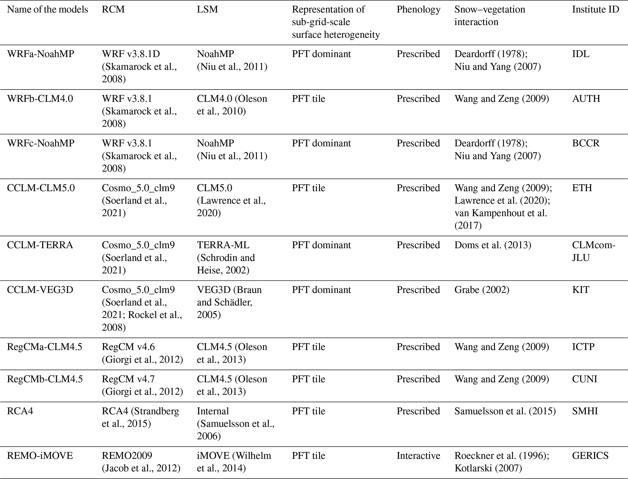
Table 1 Summary of participating regional climate models and their land surface models.

2 Data and methodology

2.1 LUCAS experiments and models

2.1.1 The LUCAS experiments

The simulations from the flagship pilot study LUCAS cover the standard EURO-CORDEX domain (Jacob et al., 2014) with a horizontal grid resolution of 0.44^∘ (around 50 km). All RCMs in LUCAS, except the RegCM model, use a rotated coordinate system, which is a cartographic projection to transform coordinates from a 3D sphere to a 2D plane (the model domain). The RegCM model applies a Lambert conformal projection (suitable for mid-latitudes) on a regular grid. Here we use outputs from the EVAL experiment, which employ standard land use and land cover maps. All simulations span the period 1986–2015 (with a spin-up period ranging from 1 up to 6 years depending on the model) and take lateral and boundary conditions from the ERA-Interim reanalysis (Dee et al., 2011). More details can be found in Davin et al. (2020).

2.1.2 Models and configurations

We use the outputs from 10 coupled surface–atmosphere RCM simulations that participated in the LUCAS project and were available at the time when we performed the analysis. The main model characteristics that are important for snow-albedo coupling are summarized in Table 1, while a detailed description of the RCMs is provided by Davin et al. (2020). The model ensemble presents five different RCMs: COSMO-CLM version 5.0-clm9 (Sørland et al., 2021), WRF version 3.8.1 (Skamarock et al., 2008), RegCM versions 4.6 and 4.7 (Giorgi et al., 2012), RCA4 (Strandberg et al., 2015), and REMO (Jacob et al., 2012). These RCMs contributed with different setups and configurations as described in Table 1. For example, the same RCM is coupled with different land surface models (LSMs): COSMO-CLM is coupled with three distinct LSMs, which are CLM5.0 (Lawrence et al., 2020), VEG3D (Breil and Schadler, 2017) and TERRA-ML (Schrodin and Heise, 2002). WRF is coupled with either CLM4.0 (Oleson et al., 2010) or NOAH-MP (Niu et al., 2011). In contrast, the same LSM is combined with different versions of RCMs. The LSM CLM4.5 (Oleson et al., 2013) is coupled with two distinct versions of RegCM (4.6 and 4.7) which also differ in their choice of convection schemes. There are also two ensemble members for which the same RCM and LSM are used (WRF and Noah-MP) but with different planetary boundary layer (PBL) schemes; these are named WRFa-NoahMP and WRFc-NoahMP in Table 1. The time resolution at which model outputs have been stored varies from one variable to another and follows the CORDEX protocol. For the analyses in the present study, we use daily and monthly model outputs for incoming shortwave radiation and snow cover. For deriving SASI, the native grid of the models was kept, minimizing data loss. The other fields were interpolated to a common 0.5^∘ × 0.5^∘ grid using Climate Data Operators (CDO) bilinear remapping.

2.1.3 Snow schemes across different land surface models

At high latitudes, the effects of snow cover on regional climate are strongly modulated by vegetation cover. The important role of forest albedo on winter and spring climate in the high latitudes is highlighted by both field campaigns, such as the Boreal Ecosystem–Atmosphere Study (BOREAS; Betts et al., 2001), and modeling studies (e.g., Betts and Ball, 1997; Betts et al., 1996, 2001; Bonan, 2008; Davin and Noblet-Ducoudré, 2010; Mooney et al., 2021), which led to the implementation of more sophisticated snow sub-models in LSMs that account for the burial of vegetation by snow. All LSMs in the LUCAS ensemble derive the fraction of vegetation buried by snow, adopting similar approaches that account for snow depth, vegetation height and snow cover fraction. The snow cover fraction f_sno depends on the snow cover accumulated at the surface over bare soil or vegetation and influences the calculation of surface albedo and fluxes. Canopy-intercepted snow does not contribute to the snow cover fraction at the ground. The CLM models (CLM4.0, CLM4.5 and CLM5.0; Swenson and Lawrence, 2012) and the internal LSM of the RCA4 model (Samuelsson et al., 2015) separately calculate the snow cover fraction during snowfall and snow melting processes, accounting for sub-grid orography when snow melting occurs. In Noah-MP, the snow cover fraction depends on snow depth, ground roughness length and snow density (Niu and Yang, 2004). In VEG3D, the snow cover fraction is internally calculated as a function of snow depth and vegetation height and is used to update surface parameters, such as albedo. However, since f_sno is not a default model output in VEG3D, the snow cover fraction has been computed for analysis purposes as a snow flag in case of a snow height above a certain threshold, producing a value that is equal to one or zero (i.e., the grid box is covered by snow or not).

Some LSMs are more sophisticated than others. CLM5.0 (Lawrence et al., 2020) and Noah-MP (Niu et al., 2007) separately treat canopy-intercepted snow and more realistically capture temperature and wind effects on snow processes. In addition, LSMs differ in the number of additional layers for snow calculation: CLM5.0 uses 12 snow layers; CLM4.0, CLM4.5 and TERRA-ML (Tölle et al., 2018) use five; Noah-MP uses three; VEG3D and iMOVE use two; and RCA4 uses one. The iMOVE model adopts the snow parameterization from the global climate model ECHAM4 (Roeckner et al., 1996) and reproduces the snow albedo as a linear function of the snow surface temperature and of the forest fraction in a grid cell, with fixed maximum and minimum snow albedo at temperatures lower than −10 ^∘C and at 0 ^∘C, respectively (Kotlarskis, 2007). In the VEG3D model, the snow scheme is based on the Canadian Land Surface Scheme (CLASS) (Verseghy, 1991) and ISBA (Douville et al., 1995) and accounts for changes in surface albedo and emissivity, as well as processes like compaction, destructive metamorphosis, the melting of snow and the freezing of liquid water. The TERRA-ML LSM model is a bulk/1D LSM that applies an infinitesimal vegetation layer on top of the soil surface and has no canopy (i.e., vegetation lays flat on the surface). Therefore, the snow always stays on top of the vegetation, and there is no snow under the trees. To correctly reproduce the effect on radiation of trees masking the ground snow, TERRA-ML applies a reduction factor for the snow albedo when vegetation (e.g., forest canopies) masks the snow.

2.2 Reanalyses and remote sensing data

Reanalysis data from ERA5-Land (Muñoz Sabater, 2019a; Muñoz Sabater et al., 2021) and MERRA-2 (Gelaro et al., 2017), as well as satellite data from the Moderate Resolution Imaging Spectroradiometer (MODIS; Hall and Riggs, 2016), are used to evaluate the modeled snow distribution and radiation in the RCMs. Specifically, we use monthly data for snow cover and incoming shortwave radiation from ERA5-Land and MERRA-2, as well as daily snow cover data from the MODIS sensors AQUA (MYD10C1) and TERRA (MOD10C1). The reanalysis data are interpolated bilinearly to the common 0.5^∘ × 0.5^∘ grid. Reanalysis data cover the time period 1986–2015 and MODIS data the period 2003–2015. Only MODIS-AQUA data are displayed in the main figures of the article, while data from MODIS-TERRA are included in the Supplement.

For MODIS data, the following processing steps are applied:

1. Since heavy cloud cover prevents a correct estimation of snow cover, data are masked by applying a threshold of 50 % to the percent of clouds in each grid cell. For comparison, we also show the results when applying a threshold of 20 % in Fig. S1 in the Supplement.

2. Only data flagged as “best”, “good” and “ok” are used, while all other data are masked.

3. Data are conservatively remapped to the common 0.5^∘ × 0.5^∘ grid. Conservative remapping is chosen due to the large difference in resolution between the original MODIS data (0.05^∘) and the target grid (0.5^∘) as it considers all grid points in the interpolation, while, for example, bilinear interpolation would only consider the neighboring grid cells of the target grid.

4. A land–sea mask is applied to make sure that only land grid points are included in the analysis. Only grid points with more than 50 % land fraction are included.

5. Data are averaged to monthly resolution.

2.3 Snow-albedo sensitivity index (SASI) and geographical scope

SASI is an index that quantifies the climate forcing due to the snow-albedo effect (Xu and Dirmeyer, 2013b). It is defined as follows:

$$\begin{array}{}\text{(1)}& \text{SASI}=\text{SW}\cdot \mathit{\sigma }\left(f_{\text{sno}}\right)\cdot \mathrm{\Delta }\mathit{\alpha },\end{array}$$

where SW is the incident shortwave radiation at the surface, σ(f_sno) is the standard deviation of snow cover fraction, which represents the interannual variation in monthly mean snow cover values, and Δα is the average difference between the albedo of a snow-covered surface and the albedo of a snow-free surface. Δα is a constant value of 0.4 as assumed in Xu and Dirmeyer (2013b). High values of SASI (given in W m⁻²), such as 10 W m⁻², indicate a strong climate forcing from the snow-albedo effect (Xu and Dirmeyer, 2013b).

To better understand geographical differences in the role of snow for land–atmosphere coupling, we focus on three sub-regions over Europe, with different climate, vegetation cover, topography and latitudes: Scandinavia (55–70^∘N, 5–30^∘E), East Europe (44–55^∘N, 16–30^∘E) and East Baltic (50–62^∘N, 20–40^∘E) (see Fig. 1). The first two regions, Scandinavia and East Europe, correspond to regions 8 and 5 of the PRUDENCE project (Prediction of Regional scenarios and Uncertainties for Defining EuropeaN Climate change risks and Effects; Christensen and Christensen, 2007). The three selected regions differ in terms of climate but also in terms of vegetation: needle-leaved evergreen forests dominate in Scandinavia, while cropland and more deciduous trees cover the other two regions. The Scandinavian region also stands out because of its geographical location stretching over high latitudes, where the incoming shortwave radiation is very small or zero during winter. In comparison with the plain region of the East Baltic region, East Europe and Scandinavia have a more complex topography as they encompass the Carpathian and Scandinavian mountains, respectively.

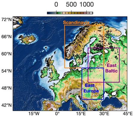
Figure 1 Map showing the location of the three regions of interest: Scandinavia (orange), East Baltic (purple) and East Europe (blue).

Figure 2 Spatial maps of snow cover for the satellite observations of MODIS-AQUA, the reanalyses of ERA5-Land and MERRA2, and the 10 RCMs from the EVAL experiment of LUCAS. Data show monthly averages from January to June over the period 1986–2015 for models and reanalyses and over 2003–2015 for satellite observations. See Fig. S2 in the Supplement for the same figure will all datasets averaged over the time period 2003–2015.

3 Results and discussion

3.1 Snow cover in Europe from satellites, reanalyses and RCMs

We start by giving an overview of spatiotemporal differences in snow cover between the different datasets. Figure 2 shows the geographical distribution of snow cover over Europe from January to June based on satellite observations averaged over the 2003–2015 period, as well as data from ERA5-Land, MERRA2 and the LUCAS models averaged over 1986–2015. The same figure with all datasets averaged over the time period 2003–2015 is presented in Fig. S2 in the Supplement. MODIS-AQUA, ERA5-Land and MERRA2 all show a similar spatiotemporal cycle, albeit with some differences in amplitude, e.g., higher snow cover in spring in ERA5-land compared to MODIS-AQUA and MERRA-2. Snow cover is high during the first months of the year when snow is accumulating (accumulation period) and then decreasing when snow is melting (ablation period). The satellite and reanalysis datasets capture the later snowmelt at higher latitudes than at mid-latitudes, showing high snow cover values during spring, while over the rest of Europe snow cover values are very low. Most of the models exhibit the same overall spatiotemporal cycle in snow cover. However, large differences exist across models regarding the amplitude and pattern of snow cover, especially during the ablation period. To facilitate further investigations into inter-model differences, we consider models by atmospheric model groups (i.e., WRF, CCLM, RegCM and others), highlighted by the different colors of the labels in Fig. 2. Large dissimilarities can appear between the members of each group. For example, in the WRF model group, WRFb-CLM4.0 has much higher values in snow cover than the other members. This is also the case for the CCLM group, with CCLM-VEG3D showing higher snow cover values than the rest of the CCLM models. For the RegCM group, the differences between the two group members are less pronounced. Comparing across atmospheric model groups shows that RegCM models tend to have snow staying longer on the ground, with higher values in snow cover in May and June compared to the other models. Generally, the comparison between the different atmospheric model groups indicates that using the same atmospheric model does not guarantee producing a similar representation of snow cover, emphasizing that the specificities of each configuration (e.g., parameterization, land surface model) can have a large impact on the representation of snow variables. These dissimilarities are not limited to snow cover and apply to other variables such as snow depth, which also exhibits large inter-model differences (see Fig. S3 in the Supplement). Such variations can have large effects on the representation of the local climate through, for example, an impact on the surface energy budget.

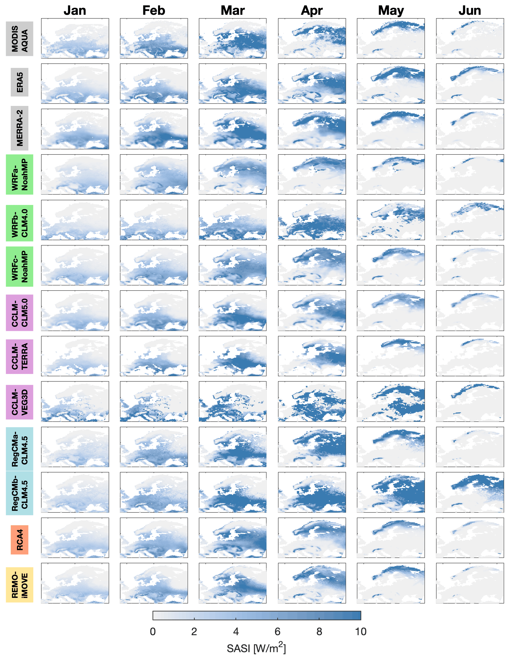
Figure 3 Spatial maps of SASI (W m⁻²) for satellite observations of MODIS-AQUA, the reanalysis of ERA5-Land and the 10 RCMs from the EVAL experiment of LUCAS from January to June, averaged over the time period 1986–2015.

3.2 SASI in satellite observations, reanalyses and RCMs over Europe

Figure 3 shows the geographical distribution of SASI over Europe from January to June for satellite observations (2003–2015), ERA5-Land, MERRA-2 and the LUCAS models (1986–2015). Focusing first on the satellite observations, MERRA-2 and ERA5-Land, an increase in SASI can be observed during the first months of the year when solar radiation increases, and snow accumulates. The maximum is reached during the ablation period in March or April, depending on the region examined, and finally SASI decreases as snow completely melts. At higher latitudes snow melts later than at mid-latitudes (see Fig. 2), causing high SASI values during spring. The SASI maximum shows a rather sharp peak in East Baltic, while it is more spread out in East Europe and in Scandinavia. This overall seasonal trend is consistent with Xu and Dirmeyer (2013b). Most of the models exhibit a similar spatiotemporal cycle in SASI as the satellite observations, ERA5-Land and MERRA-2. However, large differences can be seen across models in terms of pattern and amplitude. In March over the Carpathian Mountains, for example, SASI varies between 1 W m⁻² for WRFa-NoahMP and RCA4 and 10 W m⁻² for CCLM-CLM5.0 and RegCMa-CLM4.5. It is also noteworthy that for almost all the models, SASI is close to zero everywhere in continental Europe in May and June except for RegCMb-CLM4.5 and CCLM-VEG3D, which still have high values of SASI (∼ 10 W m⁻²).

In each atmospheric model group, simulations show large dissimilarities in terms of SASI, amplitude or pattern, especially during the ablation period. WRFa-NoahMP and WRFc-NoahMP show noticeable differences in the amplitude and pattern of SASI (Fig. 3) even though they use the same LSM and atmospheric model. The differences come from their distinct parameterizations of planetary boundary layer and convection, affecting the simulated temperature and precipitation, which in return can influence their representation of snow cover and SASI. This demonstrates the importance of atmospheric processes and their model representation for representing snow processes. Furthermore, when WRF is coupled with the LSM CLM4.0 (WRFb-CLM4.0), it shows different results compared to the simulations with Noah-MP. In WRFa-NoahMP snow melts about 1 month earlier than in WRFb-CLM4.0. Such dissimilarities also exist in the RegCM and CCLM groups. CCLM-CLM5.0, CCLM-TERRA and CCLM-VEG3D use the same RCM but different LSMs. However, in contrast to the two other CCLM configurations, CCLM-VEG3D uses a snow flag for snow cover (i.e., only indicating if snow is present or not; Sect. 2.3), likely explaining its different representation of SASI. This suggests that SASI is very sensitive to the model configurations and process parameterizations. In particular, the choice of the LSM or certain parameterizations (e.g., the convection scheme) can strongly influence the representation of the climate forcing from the snow-albedo effect. The role of the LSM in this context will be investigated further below.

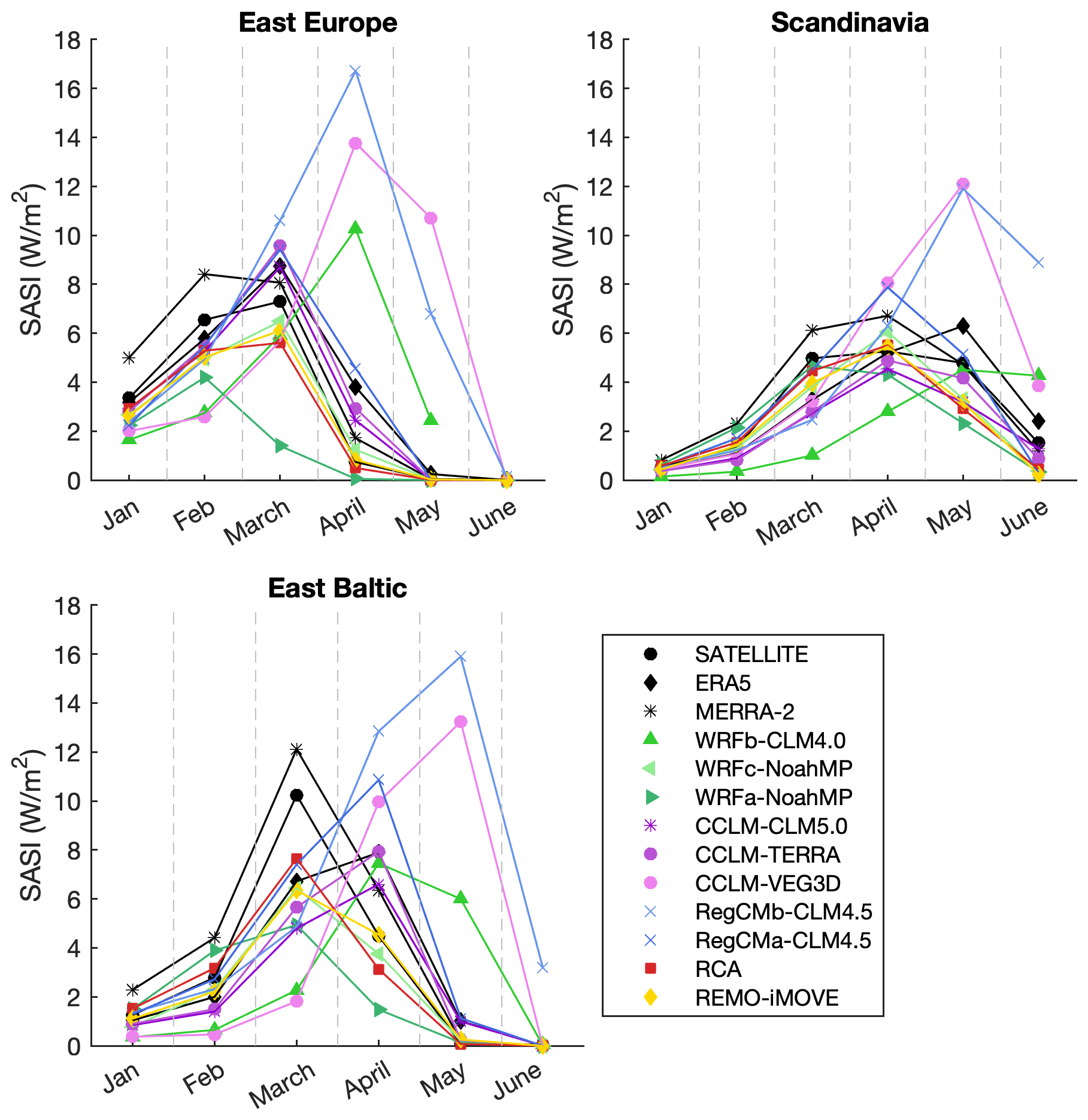
Figure 4 Time series of the spatial average of SASI for the satellite observations, the reanalysis ERA5-Land and the 10 RCMs from the EVAL experiment of LUCAS in Scandinavia, East Europe and East Baltic (see Fig. 1 for their spatial extent). Data are averaged over the time period 1986–2015.

3.3 Investigating the origin of the differences in the representation of SASI

3.3.1 Transition between the accumulation and ablation periods

To further investigate the differences in snow-albedo coupling strength between the simulations and the observation-based datasets during the accumulation and ablation periods, a time series of SASI from January to June is presented in Fig. 4 for the three sub-regions: East Europe, East Baltic and Scandinavia (see Fig. 1 for their extents). SASI values are generally higher in East Europe and East Baltic (mid-latitude regions) than in Scandinavia (high-latitude region). This confirms previous findings from Xu and Dirmeyer (2013b), who estimated higher values of SASI in mid- versus high-latitude regions in satellite observations. Part of this difference is likely due to the lower values in incoming solar radiation in Scandinavia compared to the other regions. However, even with lower SASI values at high versus middle latitudes, this result suggests that the radiative forcing due to the snow-albedo effect is not negligible over high-latitude regions in winter and spring, highlighting the importance of snow–atmosphere processes in middle and high latitudes in the Northern Hemisphere.

Returning to the comparison of the different datasets, the models and observations indicate a pronounced springtime peak in SASI in all three regions. As already mentioned, the maximum in SASI occurs during the ablation period when snow is melting. The exact timing of this transition depends on the latitude of the respective region. There is also a difference in the timing of the peak between the satellite observations, MERRA-2 and ERA5-Land, in particular over Scandinavia and East Baltic, although the amplitude is very similar. Over East Europe the peak occurs in March for both the satellite observations and ERA5-Land but in February for MERRA-2, in March (satellites, MERRA-2) or April (ERA5-Land) for East Baltic, and in April (satellites, MERRA-2) or May (ERA5-Land) for Scandinavia. The origin of these differences remains unclear, but it is not related to the difference in time period between the satellite observations and the reanalysis (see Fig. S2 for snow cover).

The LUCAS simulations also show a pronounced peak in SASI in all regions (Fig. 3); however, they do not all agree on the timing and the amplitude of the signal. This is true both within the different groups of models but also for all the simulations. For example, in the East Baltic region, some models (WRFc-NoahMP and WRFa-NoahMP) simulate a peak in March and others in April (WRFb-CLM4.0 and CCLM-CLM5.0) or even in May (RegCMb-CLM4.5 and CCLM-VEG3D). In general, RegCMb-CLM4.5 and CCLM-VEG3D tend to present the latest peak in SASI, as well as the highest amplitude in the signal. On the other hand, WRFa-NoahMP tends to produce an earlier peak and lower values of SASI, especially over East Europe. These differences might be related to snow remaining longer on the ground (Sect. 3.1) and melting later in the different models, and they will be further explored in the next section. More generally, we see that during the accumulation period, all the datasets are in better agreement compared to the ablation period (Fig. 4). For East Europe and East Baltic, the spread largely increases in March and for Scandinavia from April until the end of the season when the snow is melting.

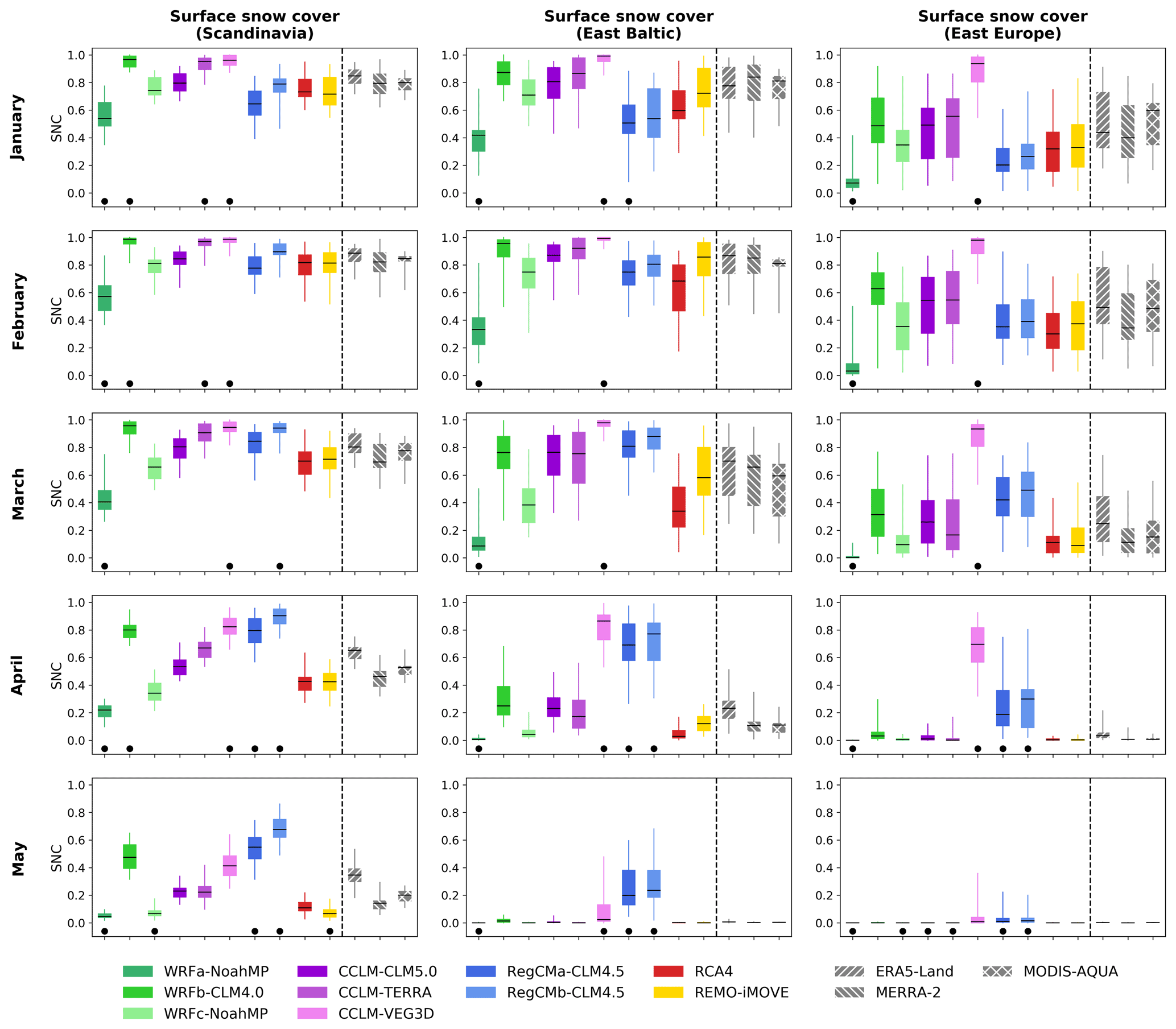
Figure 5 Snow cover for the 10 RCMs, the reanalyses of ERA5-Land and MERRA-2, and the satellite observations of MODIS-AQUA for January to May. The box-and-whisker plots show the interannual variability in snow cover over 1986–2015 for models and reanalyses and over 2003–2015 for satellite observations. Bars represent the median, boxes the interquartile range and whiskers the minimum/maximum values. Dots indicate models lying outside the range of the reference datasets of MERRA-2, ERA5-Land and MODIS-AQUA, i.e., the 25th (75th) model percentile is higher (lower) than the highest 75th (lowest 25th) quantile of the reference datasets. For satellite observations we only use data from days and pixels with less than 50 % cloud cover. See Fig. S1 in the Supplement for the same figure including data for MODIS displayed for cloud cover fraction thresholds of 50 % and 20 %.

This large model spread during the ablation period is further confirmed by examining the pattern correlation between the simulations and ERA5-Land from January to June (not shown). For many models, the correlation is high at the beginning of the season but strongly decreases in March or April when the snow starts melting. These results agree with previous studies showing the difficulties of climate models to represent snow processes during the ablation period (Essery et al., 2009). Given the dominant role of land surface over atmospheric processes during the ablation period, this suggests that the choice of the LSM is more critical for the representation of the climate forcing from the snow-albedo effect than the atmospheric model in spring. For simulating snow-covered areas at different stages of ablation, a correct representation of the landscape type is important (Pomeroy et al., 1998). In this context, it is interesting that no systematic differences can be observed between the plant functional type (PFT)-dominant versus PFT-tile models' representations of the sub-grid-scale surface heterogeneity (Table 1) as it does not seem to affect the ability of RCMs to represent snow cover or SASI. The pattern correlation (not shown) also indicates that the behavior of the RCMs is different between East Europe and East Baltic versus Scandinavia. Over the latter region, most RCMs differ from the reanalysis, as indicated by low correlations. Earlier studies showed that snow accumulates or melts very differently in an open region compared to a forested region (Jonas and Essery, 2014; Moeser et al., 2016). Our results suggest that RCMs represent snow processes better in open spaces like the East Baltic than in forest-covered regions like Scandinavia. The relationship between the representation of SASI and land cover will be further explored in the companion article, Part 2. The mountains in Scandinavia could also be a source of biases since the resolution of the RCM simulations (0.44^∘) can be considered insufficient to represent the more complex topography of Scandinavia.

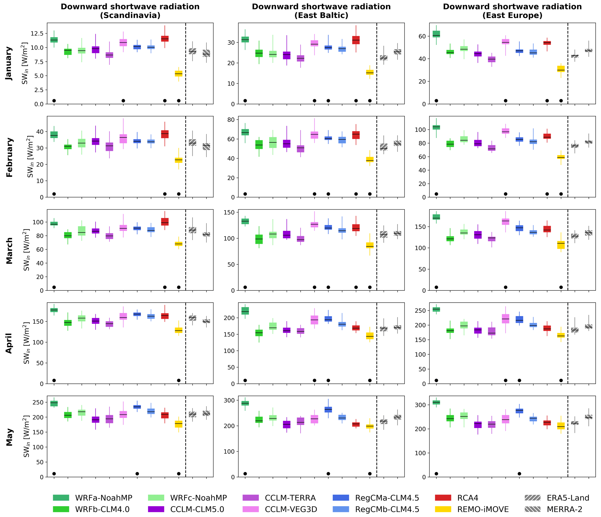
Figure 6 Downward surface shortwave radiation for the 10 RCMs, MERRA-2 and ERA5-Land for January to May. The box-and-whisker plots show the interannual variability in downward shortwave radiation over 1986–2015, with the bar representing the median, boxes the interquartile range, and whiskers the minimum/maximum values. Dots indicate models lying outside the range of the reference datasets of MERRA-2, ERA5-Land and MODIS (i.e., the 25th (75th) model percentile is higher (lower) than the highest 75th (lowest 25th) quantile of the reference datasets). See Fig. S5 in the Supplement for the same figure will all datasets averaged over the time period 2003–2015.

3.3.2 Inter-model differences in SASI

To better understand the origin of the differences in SASI across RCMs, we explore the relationship between SASI and its components, surface snow cover and shortwave radiation, during the accumulation and ablation periods. Figure 5 presents a comparison of monthly surface snow cover for the LUCAS simulations, MERRA-2, ERA5-Land and MODIS-AQUA, averaged over the three regions of interest from January to May. As shown in Sect. 3.1, differences can be observed between the reanalyses and the satellite observations as these datasets have their own limitations or biases. For example, as each reanalysis dataset is based on a different dynamical core, each model may parameterize or resolve physical processes differently (Daloz et al., 2020). The surface snow cover in East Baltic in March is ∼ 0.6 for MODIS, ∼ 0.7 for MERRA-2 and ∼ 0.8 for ERA5-Land. It is therefore important to include several reference datasets to evaluate the ability of climate models to represent snow cover and estimate the uncertainties associated with this variable. Based on Fig. 4, RegCMb-CLM4.5 and CCLM-VEG3D were identified as models with higher values in SASI during the ablation period and later peaks for all regions. Figure 5 shows that this behavior can be at least partly attributed to their representation of snow cover. During the ablation period, both tend to produce higher values of snow cover compared to the other models and to keep high values later in the season when they lie completely outside the range of the reference datasets (indicated by the black dots in Fig. 5). This is particularly striking for CCLM-VEG3D. Similarly, the low SASI peaks for WRFa-NoahMP, which also occur earlier than the peaks for other models (Fig. 4), might be related to the comparatively low values in snow cover (WRFa-NoahMP lying outside the range of the reference datasets in all months and all regions) and the small interannual snow cover variability compared to the other RCMs, particularly in East Europe (Fig. 5). The differences in snow cover are also reflected by the timing of snowmelt (reduction in snow mass) for the different RCMs (Fig. S4 in the Supplement). The models having high snow cover late in spring (RegCMb-CLM4.5 and CCLM-VEG3D) tend to have later snowmelt than the other models, while WRFa-NoahMP, showing reduced snow cover earlier than the other models, also tends to have an earlier snowmelt.

Another component of SASI is shortwave radiation at the surface, shown in Fig. 6 for the LUCAS simulations and MERRA-2 and ERA5-Land, averaged over our three regions of interest, from January to May. The comparison between the RCMs and the reanalysis shows noticeable differences for some models. Both REMO-iMOVE and WRFa-NoahMP exhibit very different results in terms of surface shortwave radiation compared to the datasets, showing much lower and higher values than the reference datasets, respectively. However, even with these discrepancies, they both reproduce SASI reasonably well.

This is confirmed by Fig. 7, showing the average correlation across models between SASI and shortwave radiation (Fig. 7a), as well as SASI and snow cover (Fig. 7b) for the LUCAS models. Scandinavia and East Baltic present similar results with significant, positive correlations between SASI and snow cover for almost all months, associated with positive but not statistically significant correlations between SASI and shortwave radiation. For East Europe, the correlation between SASI and snow cover is lower and not significant in January and February but remains high and significant the rest of the time period. In parallel, the correlation between SASI and downward shortwave radiation at the surface is negative for almost all months (but not statistically significant). Overall, high and significant correlations often appear between SASI and snow cover for the three regions from January to June. On the other hand, the correlations between SASI and shortwave radiation are low and usually not significant. This indicates that the differences in the representation of the forcing from the snow-albedo effect are mostly driven by differences in the representation of snow cover in the models.

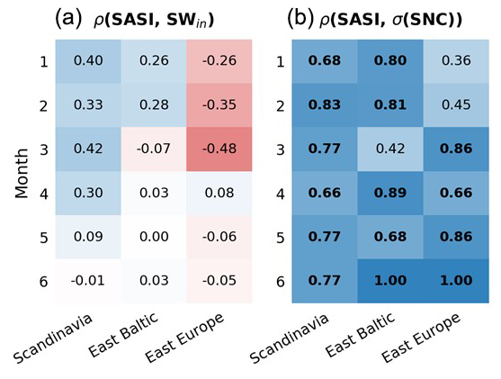
Figure 7 Pearson correlation between SASI and shortwave radiation (a) and SASI and standard deviation of snow cover (b) calculated across RCMs for the three regions – Scandinavia, East Baltic and East Europe – for the months of January to June during 1986–2015. The values represent the variable (shortwave radiation or variability in snow cover) to which the inter-model variability in SASI is predominantly related. Bold values indicate statistical significance at the 0.05 level (two-tailed p value).

4 Conclusion

Previous work has demonstrated the difficulty for climate models to represent snow variables or processes, such as snow cover and depth (Matiu et al., 2020), or snow–atmosphere processes, such as the snow-albedo feedback (SAF; Fletcher et al., 2015), but the origin of the differences between models is not clear yet. In this work, we focus on the ability of RCMs to simulate the radiative forcing associated with snow cover anomalies in winter and spring over Europe and explore the origin of the differences across the RCMs. The radiative forcing associated with snow cover anomalies is represented by the index SASI (Xu and Dirmeyer, 2013b), which quantifies the strength of the coupling between snow and surface net shortwave radiation. A total of 10 RCMs from the CORDEX flagship pilot study LUCAS are compared to satellite observations and the reanalysis datasets ERA5-Land and MERRA-2. These simulations are part of the control experiment of LUCAS.

The results show that climate models are able to reproduce well some of the SASI characteristics (e.g., existence of a peak, amplitude of the peak) compared to reanalyses and satellite observations, even if large differences appear between the RCMs, for all groups of models. The climate models' ability to represent SASI is highly related to their representation of snow cover, which can be difficult to represent for climate models. Our results also suggest that the models' capability highly differs between the accumulation and ablation periods. Most models have much lower agreement with reanalyses and satellite observations in the ablation period, indicating a systematic bias regarding snow cover in spring, in turn pointing towards a bias from LSMs. This bias seems to be common to most LSMs even if they are based on different assumptions and parameterizations. It is also interesting that even though CCLM-TERRA is not as advanced in terms of snow modeling compared to the other models, it still manages to represent SASI reasonably well over Europe. In addition, there were no systematic differences between the PFT-dominant versus PFT-tile models (Table 1) as it does not seem to affect the ability of RCMs to represent snow cover or SASI. Taking advantage of the different configurations of the LUCAS simulations, we have also explored the role of distinct parts of the models in their ability to represent SASI. This work has emphasized the role of the LSMs, but other components can also play an important role. For example, WRFc-NoahMP and WRFa-NoahMP, even though using the same RCM and LSM, show noticeable differences in the amplitude and pattern of SASI. Their differences in parameterizations (planetary boundary layer and convection) are certainly affecting the way they represent SASI, highlighting the impact of such choices and the role of atmospheric processes.

Mid- and high-latitude areas are also specifically examined looking at three sub-regions: Scandinavia, East Europe and East Baltic. The comparison of the three sub-regions shows the difficulties for models to simulate SASI over Scandinavia during the accumulation and ablation periods. The simulation of snow processes in a forested region is more challenging than in an open region (Jonas and Essery, 2014; Moeser et al., 2016). Thus, climate models can potentially have more difficulties representing snow processes in forest-covered regions like Scandinavia compared to open-land regions like East Baltic. The relationship between the representation of SASI and land cover will be further explored in the companion article (Part 2), analyzing the other LUCAS experiments: GRASS and FOREST. Finally, the comparison of mid- versus high-latitude regions shows slightly higher values of SASI over the mid-latitude regions in satellite observations, ERA5-Land, MERRA-2 and most of the RCMs. This confirms previous findings from Xu and Dirmeyer (2013b), who estimated higher values of SASI in mid- versus high-latitude regions in satellite observations. Our results also suggest that the climate forcing due to the snow-albedo effect is not negligible over high-latitude regions in winter and spring. This is important since often the land–atmosphere coupling is considered weaker at higher latitudes, but it is also possible that this coupling happens through snow and is therefore underestimated.

Although it is difficult to identify the origin of the bias in the RCMs, an increase in spatial resolution might improve the simulation of snow cover and therefore the representation of SASI. For example, over Scandinavia, an increase in spatial resolution would provide a better representation of the complex topography of the region, as well as its forested areas, which may lead to an improved simulation of the coupling between snow and albedo. The coming phases of LUCAS could help answer this question as they will produce simulations at higher spatial resolutions, 12 km in phase 2 and convection-permitting (< 3 km) in phase 3.