the Creative Commons Attribution 4.0 License.
the Creative Commons Attribution 4.0 License.
 | 13 Jun 2022
A leading-edge-based method for correction of slope-induced errors in ice-sheet heights derived from radar altimetry
Weiran Li
Cornelis Slobbe
Stef Lhermitte
Satellite radar altimetry has been an important tool for cryospheric applications such as measuring ice-sheet height or assessing anomalies in snow and ice properties (e.g. the extensive melt in Greenland in 2012). Although accurate height measurements are key for such applications, slope-induced errors due to undulating topography within the kilometre-wide beam-limited footprint can cause multi-metre errors. Two main correction methods that have been developed (referred to as the slope- and point-based methods) neglect either the actual topography or the actual footprint that can be estimated by a combination of the leading edge and topography. Therefore, a leading edge point-based (LEPTA) method is presented that corrects for the slope-induced error by including the leading edge information of the radar waveform to determine the impact point. The principle of the method is that only the points on the ground that are within the range determined by the beginning and end of the leading edge are used to determine the impact point. Benchmarking of the LEPTA method against the slope- and point-based methods based on CryoSat-2 Low Resolution Mode (LRM) acquisitions over Greenland in 2019 shows that, when compared to ICESat-2 observations, the LEPTA method has a stable performance both in the flat, interior regions of Greenland and in regions with more complex topography. The median difference between the slope-corrected CryoSat-2 heights using LEPTA and the ICESat-2 heights is at the millimetre level, whereas the slope and point-based methods can have a 0.21 and 0.48 m difference, respectively, and the Level-2I (L2I) data provided by ESA have a 0.01 m difference. The median absolute deviation of height differences between CryoSat-2 and ICESat-2, which we use as an indicator of the variation in errors, is also the lowest for LEPTA (0.09 m) in comparison to the aforementioned methods (0.19 m for slope method and 0.10 m for point-based method) and ESA Level-2 data (0.14 m). Although ESA Level-2 products and the point-based method have good performance in either the median or the median absolute deviation, LEPTA shows a good performance in both metrics. Based on that, we recommend considering LEPTA for obtaining accurate height measurements with radar altimetry data, especially towards the margins of the LRM coverage where the surface slopes increase.
- Article
(4457 KB) - Full-text XML
- BibTeX
- EndNote


Satellite radar altimetry is a key tool for assessing the status and dynamics of the cryosphere as it allows constructing digital elevation models (DEMs) (Slater et al., 2018), deriving height change in ice sheets (Hurkmans et al., 2012; Helm et al., 2014a), understanding seasonal variations in snow (Adodo et al., 2018), and estimating snowpack properties (Lacroix et al., 2008). To obtain accurate information on heights, altimetry processing involves correction for instrument errors, atmospheric effects, tidal effects, and slope-induced errors (Helm et al., 2014a; Hai et al., 2021). Of crucial importance is the correction for slope-induced errors as they can affect the obtained height measurements significantly. For example, according to the error propagation in Brenner et al. (1983), the CryoSat-2 satellite at an altitude of 717 km can give a vertical offset of approximately 39 m and a horizontal offset of 7.5 km when measuring heights of a terrain with a 0.6∘ slope.
To correct for the slope-induced errors, different methods have been developed (Brenner et al., 1983; Remy et al., 1989; Bamber, 1994; Roemer et al., 2007). The most widely used methods involve both a correction to the height and a relocation of the satellite measurement location from the nadir to the expected impact point (i.e. the radar reflection point) on the terrain. Two implementations of this so-called “relocation method” are known as the “slope” method and the “point-based” method (Bamber, 1994; Roemer et al., 2007). The slope method assumes constant surface slope parameters within the beam-limited altimeter footprint and calculates the relocated latitude, longitude, and height according to trigonometry (Levinsen et al., 2016). The point-based method uses a topographic model within the beam-limited satellite footprint and searches for minimum range between the satellite and a surface area in the size of the pulse-limited footprint (Roemer et al., 2007; Levinsen et al., 2016).
Although both methods have been refined and applied with reliable results, they both show methodological shortcomings. The slope method, for example, tends to ignore the local topography within the footprint and therefore may not be accurate enough in undulating areas (Levinsen et al., 2016). The point-based method of Roemer et al. (2007), on the other hand, is more accurate in the undulating regions (Roemer et al., 2007; Levinsen et al., 2016) as it considers the detailed topography, but by assuming a fixed footprint size, it neglects the actual footprint illuminated by the satellite on the terrain. For example, by taking the averaged range within the assumed footprint, this method may ignore part of the terrain that actually contributes to the return signal or assumes that part of the terrain not visible to the satellite could contribute to the return signal (Fig. 1). The recent availability of high-resolution DEM products provides the opportunity to determine the part of the terrain contributing to the rise of the leading edge and therefore can determine the actual footprint of the radar altimeter. To overcome the shortcomings of both methods, we present a leading edge point-based (LEPTA) method that exploits high-resolution DEM information to correct for the slope-induced error by including the leading edge information of the radar waveform to determine the impact point. The principle of the method is that only the points on the ground that are actually within the range interval determined by the beginning and end of the leading edge are used to compute the impact point.
The paper is organised as follows. Section 2 describes the data used for radar altimetric processing and assessment of the results. In Sect. 3, the different methods used for the correction of the slope-induced errors as well as the assessment workflow are introduced. To assess the performance of the LEPTA method, we apply it to all CryoSat-2 Low Resolution Mode (LRM) acquisitions over Greenland in 2019 and benchmark it to the slope and point-based methods by comparing it with laser altimeter ICESat-2 height measurements. In Sects. 4 and 5 we present, analyse, and discuss the results. Finally, we conclude by emphasising the main findings.
2.1 CryoSat-2 observations
In the interior of the Greenland ice sheet, data acquired by CryoSat-2 are in LRM. LRM is the conventional pulse-limited mode that requires correction for slope-induced errors. The pulse-limited LRM footprint is approximately 1.65 km in diameter, and the beam-limited footprint is approximately 14.39 km in diameter (Hai et al., 2021). Our evaluation employs all data acquired from 1 January to 31 December 2019, resulting in approximately 2.2×10⁶ measurements. In particular, we use Level-1b (L1b) Baseline D data (European Space Agency, 2019a; Meloni et al., 2020).
To process the waveform information and obtain height estimations, the L1b waveforms are retracked using the offset centre of gravity (OCOG) method (Wingham et al., 1986) documented in Bamber (1994). We use OCOG because of its precision and robustness (Bamber, 1994; Schröder et al., 2019). According to Davis (1997), a 10 % threshold is ideal for detecting ice-sheet height change (or strong volume scattering; Aublanc et al., 2018), a 20 % threshold is the most appropriate for estimating the absolute or true ice-sheet height, and a 50 % threshold is the most appropriate for estimating the absolute height when the waveform is dominated by surface scattering (Davis, 1997; Aublanc et al., 2018). In this study, we follow the recommendation of Davis (1997) and use a 20 % threshold to obtain estimates of the true ice-sheet elevation. This allows a comparison with ICESat-2 data. Aublanc et al. (2018), who used a 25 % threshold, highlighted that this choice is a compromise between pure surface scattering (in which case the threshold should be around 50 %) and volume scattering (10 %). In the first case, one would underestimate the true elevation and in the other overestimate it. Hence, as pointed out by Davis (1997), “the 20 % retracking point provides a reasonable estimate of the true ice-sheet elevation in only an average sense”. In addition, waveforms are removed if they meet one of the following empirically derived criteria: (i) the integrated normalised power exceeds 150; (ii) the normalised power in the first 10 range bins is larger than 0.2; or (iii) no peaks are identified in the waveform.
To benchmark our results, Level-2I (L2I) height data obtained with the OCOG retracker from the European Space Agency (2019b) are used. In the L2I products the slope-induced error is corrected with the Helm et al. (2014b) DEM, which has a resolution of 1 km×1 km (Helm et al., 2014a). To enable a fair comparison with our in-house-processed L2I data, all L2I height measurements are removed for which the waveforms meet one of the criteria mentioned above.
2.2 ArcticDEM
To compute a correction for the slope-induced errors, a DEM is needed. Here, the slope method uses a low-resolution DEM as it assumes a constant slope within the pulse-limited footprint (Levinsen et al., 2016). On the contrary, the point-based methods (i.e. LEPTA and the point-based method proposed by Roemer et al., 2007) require DEMs with higher resolution to provide the full information of the local terrain.
In this study, ArcticDEM is used as reference DEM as it is constructed from recent stereo satellite imagery and is available in high resolution (2 m×2 m) (Porter et al., 2018). The systematic error in ArcticDEM is less than 5 m (Noh and Howat, 2015), and the DEM has been updated since 2016. ArcticDEM is low-pass filtered to a 2 km resolution by applying a block-mean filter for the slope-based method and to a 100 m resolution for the point-based and LEPTA methods. The use of a 100 m resolution instead of 2 m is a compromise for computational efficiency. To assess the impact of DEM resolution on the correction methods, we vary the resolutions from 100 m (200 m for the slope method, for computational efficiency) to 900 m with a 100 m interval and from 1 to 8 km with a 1 km interval.
2.3 ICESat-2 observations
For validation of the different slope correction methods, the ICESat-2 L3A Land Ice Height (ATL06) product (Smith et al., 2020a) is used. ICESat-2 uses the Advanced Topographic Laser Altimeter System (ATLAS), which emits green light pulses and counts the received photons (Abdalati et al., 2010). The laser beams are configured in a 2×3 array. The distance between and within beam pairs is ∼3.3 km and ∼90 m, respectively (Smith et al., 2019). The along-track resolution of the land ice height product is ∼20 m (Smith et al., 2020b). The ATL06 products have a known geolocation accuracy (or bias) of less than 10 m (National Snow and Ice Data Center (NSIDC), 2021). A comparison between ICESat-2 and ArcticDEM is shown in Appendix A. The results show that the median ICESat-2 height for the different beam pairs is up to 0.21 m higher than ArcticDEM. The median absolute deviation of the differences is 0.72 m for all beam pairs.
3.1 Slope correction methods
The different slope-induced error correction methods are conceptually illustrated in Fig. 1. The impact points estimated from the slope method, the point-based method, and LEPTA are represented by Ps, Pp, and Pl. The “low-resolution DEM” (2 km) is only used by the slope method, whereas the point-based method and LEPTA use a “high-resolution DEM” (100 m). The slope method computes a correction based on the surface slopes obtained from a DEM, whereas the point-based method and LEPTA are based on the range between the satellite and the terrain.
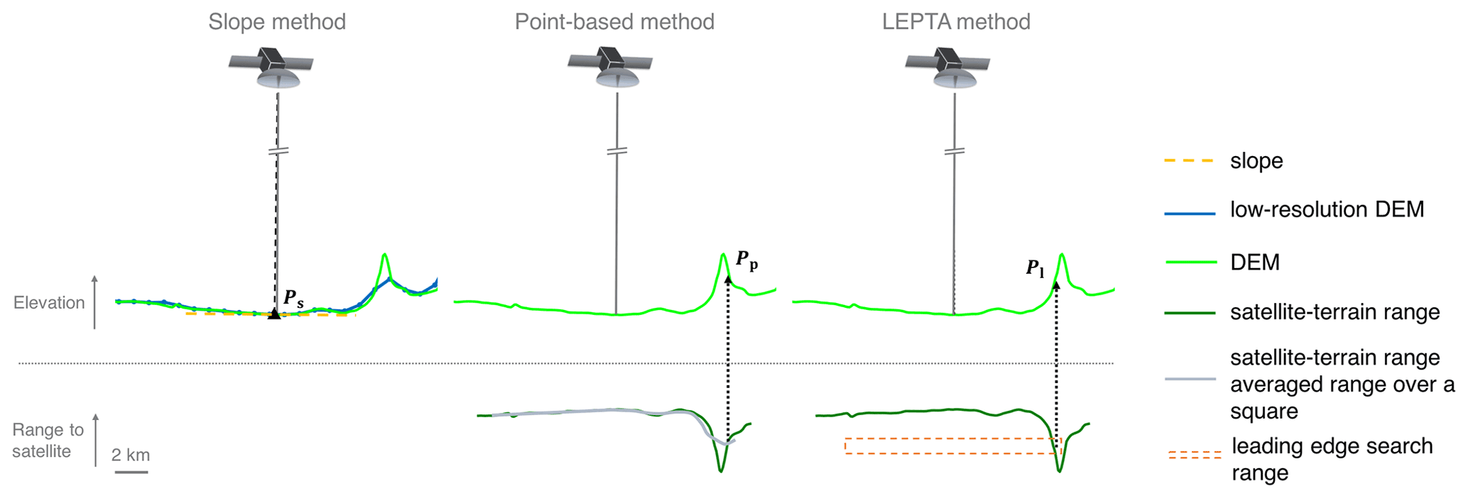
Figure 1Conceptual illustration of different slope-induced error correction methods. The impact points estimated from the slope method, the point-based method, and LEPTA are represented by Ps, Pp, and Pl. The slope method computes a correction based on the surface slopes obtained from a DEM, whereas the point-based method and LEPTA are based on the range between the satellite and the terrain.
3.1.1 Slope correction method
The slope method uses the slope of the low-resolution DEM at the nadir point to compute the impact point. It assumes that the slope within the CryoSat-2 pulse-limited footprint is constant and is defined by direction θ and magnitude Φ (Cooper, 1989; Bamber, 1994). In our implementation, θ and Φ are computed in the same map projection and grid as ArcticDEM. The gridded θ and Φ are then interpolated to the satellite nadir point. The corrected height (hC), corresponding to the height of the impact point Ps, can then be obtained by (Bamber, 1994)
where
R represents the retracked range, a and e the semi-major axis and eccentricity of the reference ellipsoid being used, and ϕ the latitude of the satellite. The corrected location of the impact point in latitude ϕC and longitude λC (in radians) is computed as
where X and Y define the position of the satellite in Cartesian coordinates:
and
Application of the slope method in Fig. 1 shows that the impact point will be assumed at the position Ps. Inaccuracies usually occur when this method is applied to complex terrains due to the simplification of the complex topography to a constant slope (Levinsen et al., 2016).
3.1.2 Point-based correction method
The point-based method directly uses the topographic information from the a priori DEM to find the impact point (Pp). It does so by minimising the mean distance to the satellite over a pre-defined fixed-size rectangular footprint area (e.g. 1.65 km×1.65 km in Hai et al., 2021). Assuming the pre-defined rectangular footprint with area A consists of n DEM grid cells, is computed by (Roemer et al., 2007)
where APj and are the area of and range to each grid cell j. The point for which is minimal is referred to as Pp with latitude ϕc and longitude λc. The range between the satellite and Pp is referred to as rp. In line with Roemer et al. (2007), we use the 100 m DEM to find an approximate position. The final point is obtained by a second search in the vicinity of the approximate position for which we use an up-sampled DEM of 10 m×10 m. The corrected height hC is computed as (Roemer et al., 2007)
where hN is the surface height of the nadir point relative to the reference ellipsoid (i.e. the ellipsoidal height of the satellite hS minus the retracked range R) and hI is the DEM height of Pp. Equation (11) also shows, however, that this approach can take DEM points into account that actually do not contribute to the rise of the leading edge (i.e. points that fall outside the pulse-limited footprint).
3.1.3 Leading edge point-based (LEPTA) correction method
The LEPTA method is similar to the point-based method as it also uses the topographic information from the a priori DEM to find the impact point (Pl) but differs in the search method of the impact point. Instead of pre-defining a fixed pulse-limited footprint size, the LEPTA method identifies the parts of the terrain within the beam-limited satellite footprint that contribute to the rise of the leading edge. To identify these points, we use a beam-limited satellite footprint of 14.39 km×14.39 km (Hai et al., 2021) centred around the nadir point and a search range bounded by rbegin and rend:
where r1% and r90% refer to the retracked ranges obtained using a 1 % and 90 % threshold retracker (Davis, 1997), respectively; r20% is the OCOG retracked range using a 20 % threshold to obtain the firn–air interface; and Δr is a user-defined threshold. Δr is used to avoid the search range (rend−rbegin) becoming unrealistically large. For all experiments, we use a value of 1.25 m based on an empirical optimisation of Δr. If no DEM grid points are identified within the search range, we add the difference between the range to the closest DEM point and rbegin to rbegin and rend.
The location of Pl is computed as the average of all identified DEM grid points K. Finally, the corrected height hC is computed by
where is the ellipsoidal height of the ith identified DEM grid point and the range between the satellite and the ith identified DEM grid point. By using averaging to compute Pl, it is theoretically possible that the average location is outside the actual pulse-limited footprint (e.g. when the impact points form a doughnut shape or two equally large but disjointed sets of points). These occurrences can be easily identified.
One of the advantages of the LEPTA method compared to the point-based method is that it includes points that contribute to the rise of the leading edge signal but are outside the fixed (square) pulse-limited footprint and rejects points that do not contribute to the rise of the leading edge signal but are inside the pre-defined pulse-limited footprint. An additional advantage of LEPTA is that it does not apply the recursive computation process as the point-based method; therefore it speeds up the processing.
3.2 Performance assessment
To assess the performance of the LEPTA method, we benchmark the different methods by comparing their accuracy relative to reference data. First, we directly compare the corrected heights (hC) for each method with the reference height from the 100 m ArcticDEM. To compare hC with the DEM, we bi-linearly interpolate the DEM heights to the CryoSat-2 locations (hDEMC). Then, the CryoSat-2 measurements are grouped in 25 km×25 km tiles. For each tile, we compute the median and median absolute deviation of the hC−hDEMC values. This assessment cannot be considered a validation as ArcticDEM is not an independent dataset. However, it is insightful, especially when the CryoSat-2 points do not have an ICESat-2 point nearby.
Secondly, we compare the corrected height measurements with the ICESat-2 heights for each method. This comparison is carried out per month; i.e. we compare the CryoSat-2 heights acquired in a particular month to the ICESat-2 heights acquired in the same month. For each point, we first identify all ICESat-2 points within 50 m of the CryoSat-2 point. If ICESat-2 points are available in each quadrant surrounding the CryoSat-2 point, the ICESat-2 heights are interpolated to the CryoSat-2 point using a natural-neighbour interpolation (hICE2). Otherwise a nearest-neighbour interpolation is applied. A natural-neighbour interpolation provides a smoother solution (Bobach, 2009) yet requires weighting functions based on the surrounding points. To correct for the height difference between the locations of the CryoSat-2 and ICESat-2 points over a potentially sloping terrain, we apply a correction computed as the height difference between the 100 m ArcticDEM evaluated at the CryoSat-2 (hDEMC) and ICESat-2 (hDEMI) locations. Hence, the differences between the CryoSat-2 and ICESat-2 heights (Δh) become
Similarly to the comparison with ArcticDEM, we compute the median and median absolute deviation of Δh for each 25 km×25 km tile.
When benchmarking the methods, two aspects of accuracy are assessed. First, we determine the difference between the slope-corrected CryoSat-2 measurements and the reference heights (hDEMC or hICE2) using standard statistical parameters (median, median absolute deviation, mean, and standard deviation). Second, we assess the variability in the statistics for the different methods. The statistical parameters are computed with and without outliers. Cumulative functions are provided mainly to visualise the percentiles that indicate the distribution of the results and determine the outliers. Here, we consider hC−hDEM or Δh outside the 10th–90th percentile range as an outlier. Probability distribution functions are provided to visualise the overall distribution of results. The skewness parameter is provided as long tails of the probability distribution are not completely visualised. In addition, tiles including fewer than 10 measurements are rejected for visualisation and interpretation as the statistics of these tiles do not represent sufficient data and cannot be informative.
3.3 Sensitivity analysis
The LEPTA method is potentially sensitive to (i) the definition of rend and rbegin and hence Δr (Eqs. 13 and 14), (ii) a potential bias in the DEM, and (iii) the resolution of the DEM. Another aspect that may impact the height estimates of all methods is the adopted OCOG threshold. To assess how our choices impact the results, we conduct a number of sensitivity analyses in which we
-
vary Δr (Eqs. 13 and 14) from 0.5 to 5 m in steps of 0.5 m to define an optimal choice;
-
vary the adopted OCOG threshold to determine R and hence hN (Eq. 16) from 10 % to 90 % in steps of 20 %, using an optimal choice of Δr for LEPTA;
-
add a bias to the DEM from −7.5 to 2.5 m in steps of 2.5 m, using a 20 % OCOG threshold and an optimal choice of Δr for LEPTA;
-
vary the DEM resolution from 200 to 900 m in steps of 100 m and from 1 to 8 km in steps of 1 km, using a 20 % OCOG threshold and an optimal choice of Δr for LEPTA.
4.1 Comparison with ArcticDEM
The cumulative distribution of hC−hDEMC for all methods (Fig. 2a) shows that most values are within the [−1.0, 3.0] m interval (as shown by 10th and 90th percentiles), although outliers have an impact on the interpretation of the results. These outliers have most impact on the overall standard deviation and skewness of hC−hDEMC, as shown in Table 1 and Fig. 3. Although the distribution curves show a positive bias, the skewness is negative for all methods, showing more or larger negative outliers, as also shown in Fig. B1. Comparison of the methods, however, shows that LEPTA is least affected by such negative outliers.
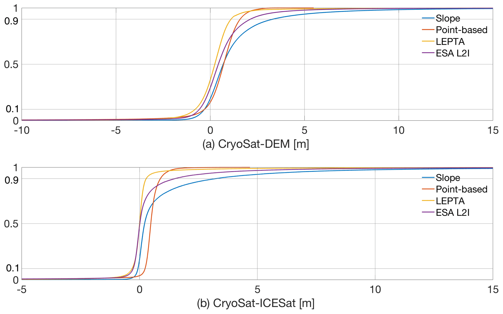
Figure 2Cumulative distribution figures of (a) the difference between CryoSat-2 and ArcticDEM (hC−hDEM) and (b) the difference between CryoSat-2 and ICESat-2 (Δh), including outliers. The 10th and 90th percentiles are shown in the figures for outlier removal. For visualisation, the x axis is restricted to [−10, 15] m for (a) and to [−5, 15] m for (b).
Table 1Statistics of the height difference between slope-corrected CryoSat-2 measurements and ArcticDEM and ICESat-2 (hC−hDEMC or Δh as computed by Eq. 16). Height statistics are in unit of metres. The parameters are shown with and without outliers (referred to as w/ outlier and w/o outlier) using 10th and 90th percentiles. E, S, P and L represent ESA L2I, slope method, point-based method and LEPTA, respectively.

Removing the outliers significantly reduces the standard deviation of hC−hDEMC and skewness for all methods and brings the mean closer to the median. Comparison of the mean and median values (Table 1) and probability distribution (Fig. 3a) moreover indicates that LEPTA performs better than other methods when compared with ArcticDEM, with a mean height difference of 0.22 m and a median difference of 0.24 m. The slope method results in the largest mean difference of 0.87 m, while the point-based method gives the largest median of 0.71 m. The standard deviation (0.46 m) and median absolute deviation (0.34 m) from LEPTA are also the smallest, the same as those obtained from the point-based method. The largest hC−hDEMC deviation values after outlier removal are given by the slope method, with the standard deviation being 0.82 m and median absolute deviation being 0.50 m. An additional note is that the mean and median from all methods are positive, which implies that the heights obtained by these methods are generally higher than ArcticDEM heights.
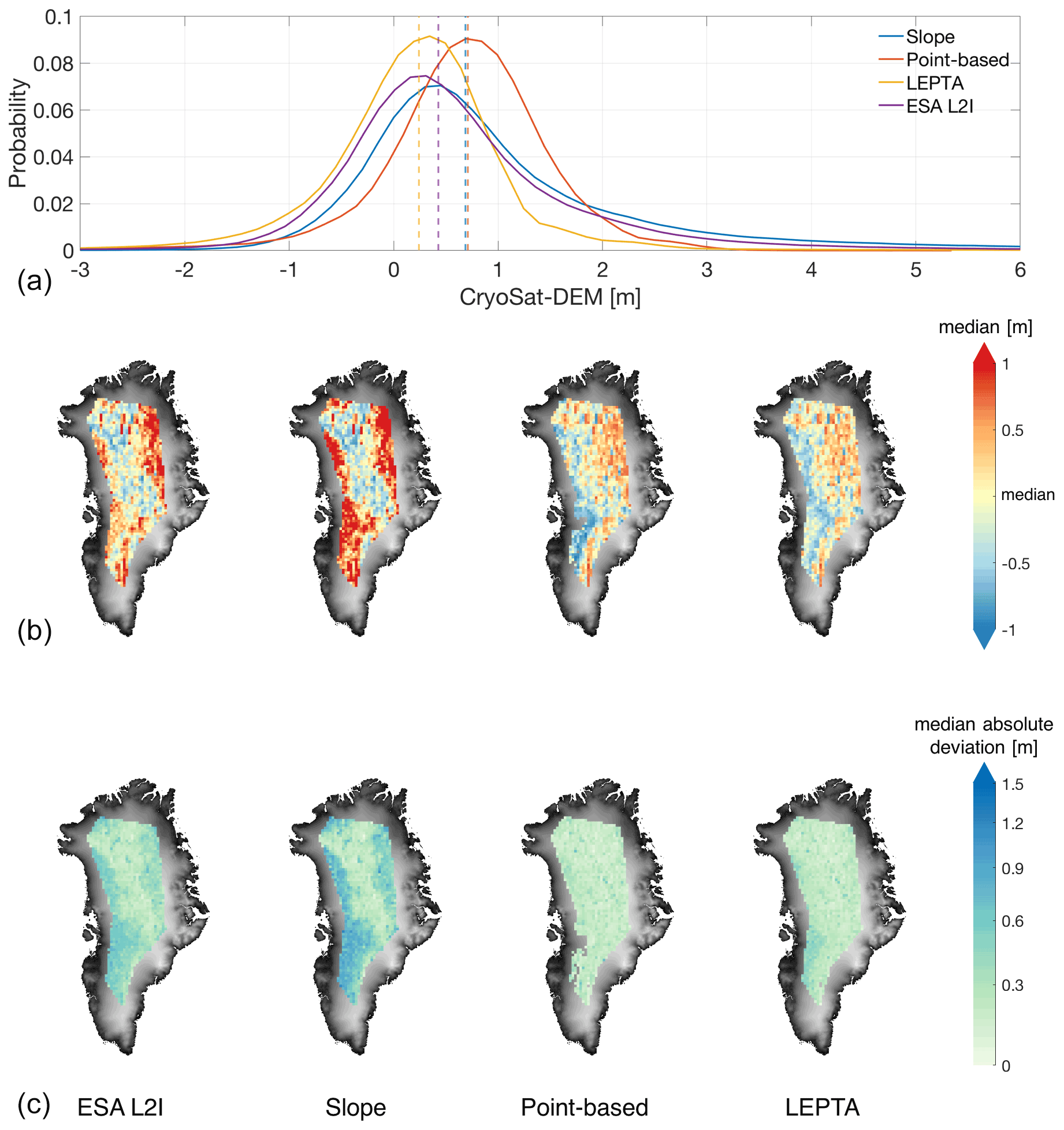
Figure 3(a) Probability distribution of height difference between CryoSat-2 and the ArcticDEM, before removing the outliers with 10th and 90th percentiles. The probability distribution is plotted with all data samples but restricted to [−3 m, 6 m] for visualisation (for better illustration of the skewness and large outliers, please refer to Appendix B). Vertical lines show median value per method. (b, c) Spatial distribution of median and median absolute deviation of the height difference per tile of 25 km×25 km, after removing the outliers. To enhance the visibility of the maps, the median value of each method is subtracted in (b). The colours of the median absolute deviation plots are on a logarithmic scale to enhance contrast. The spatial distribution results from left to right are obtained by ESA L2I products, the slope method, the point-based method, and LEPTA, with the 1 km×1 km DEM covering Greenland (Helm et al., 2014a, b) as background.
Comparison of the spatial patterns of median and median absolute deviation (Fig. 3) shows large spatial differences in both pattern and magnitude among the different methods. In general, the largest median and median absolute deviation values occur near the margins of the LRM coverage, where the terrain is steeper. For the point-based method and LEPTA, the median values on the western side are generally lower than on the eastern side. This spatial pattern is similar to that of the differences between ICESat-2 and ArcticDEM (shown in Fig. A1). For ESA L2I products and the slope method, the largest median values occur on both the eastern and the western sides of Greenland, and those from the slope method largely exceed those of the ESA L2I products, the point-based method, and LEPTA. So far, we lack a conclusive explanation for the spatial differences between the methods. Regarding the median absolute deviation values, we observe in general higher values on the western side of the ice sheet than in the interior. For the ESA L2I products and the slope method, the median absolute deviation values are also high on the eastern side. These median absolute deviation values show that topography affects the different performances of the methods, and the point-based method and LEPTA are less affected on the eastern side. In addition, for the point-based method, removing the outliers results in the most missing data close to Jakobshavn Isbræ. Combining the statistics in Table 1 and the spatial distribution of median and median absolute deviation in Fig. 3, it can be concluded that LEPTA performs best when compared with ArcticDEM.
Using averaging in Eq. (15) to compute Pl results in 5.2 % of the impact points being outside the actual footprint. Removing these points as “unreliable data” minimally affects the median and mean (0.26 and 0.25 m) but improves the median absolute deviation (0.32 m) and standard deviation (0.40 m).
4.2 Validation with ICESat-2 observations
Comparison of CryoSat-2 and ICESat-2 heights (Fig. 2b) shows again the impact of outliers on the results, although the outliers are generally lower than for the ArcticDEM comparison. ESA L2I products, the point-based method, and LEPTA have more impacts from negative outliers, while the slope method results in more positive outliers.
With the outliers removed, the standard deviation of Δh values from all methods is greatly reduced, especially for the ESA L2I and slope method, which show the largest outliers (Fig. 2b). The lowest median (0.00 m), mean (0.00 m), median absolute deviation (0.09 m), and standard deviation (0.13 m) of Δh are obtained by LEPTA, showing that the LEPTA method again outperforms the other methods. The largest median (0.48 m) is obtained by the point-based method, and the largest mean (0.51 m), median absolute deviation (0.19 m), and standard deviation (0.70 m) are from the slope method.
The comparison of the height differences between CryoSat-2 vs. ArcticDEM and CryoSat-2 vs. ICESat-2 shows moreover that the height differences with ICESat-2 are smaller, probably due to the better quality of ICESat-2 data compared to ArcticDEM and the longer time gap between CryoSat-2 and ArcticDEM, as satellite imagery data for generating ArcticDEM have been gathered since 2007 (Noh and Howat, 2017; Howat et al., 2019) and co-registered to ICESat since before 2009, whereas ICESat-2 measurements were obtained in the same month as CryoSat-2 data. The comparison between CryoSat-2 and ICESat-2 also results in fewer data points as not all CryoSat-2 measurements have corresponding nearby ICESat-2 measurements within the 50 m criterion.
The spatial distribution of the median and median absolute deviation of Δh (Fig. 4) shows clear spatial patterns. For the ESA L2I products, the slope method, and the point-based method, the median differences with respect to the overall median difference are generally negative (positive) in the central part (margins of the LRM zone). For LEPTA, the variability in negative or positive differences is smaller (especially vs. ESA L2I and the slope method) but with a slightly reversed pattern. This reversed pattern can be explained by LEPTA's definition of rbegin and rend that may result in an asymmetry around r20% that can spatially vary. Figure 4 also shows that LEPTA has the lowest spatial variability in the median absolute deviation, whereas the slope method shows the largest contrast between the interior and the margins of the LRM zone.
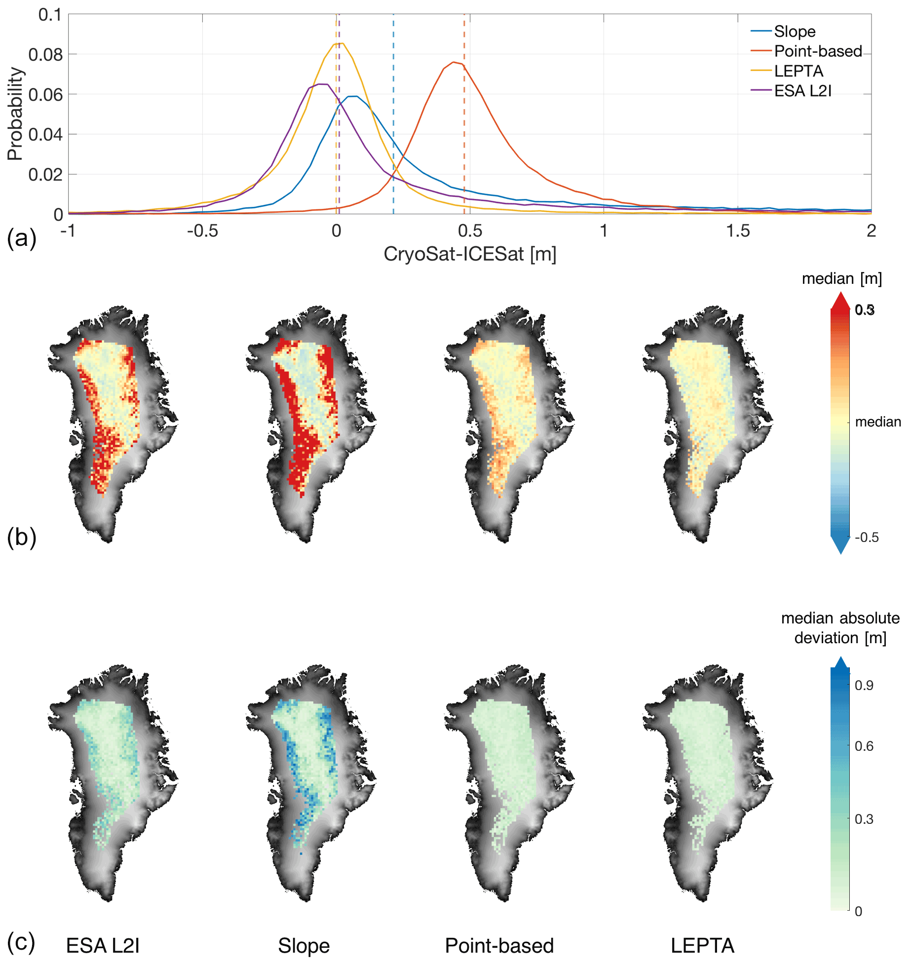
Figure 4(a) Probability distribution of height difference between CryoSat-2 and the ICESat-2, before removing the outliers. The probability distribution is plotted with all data samples but restricted to [−1 m, 2 m] for visualisation (for better illustration of the skewness and large outliers, please refer to Appendix B). Vertical lines show the median value per method. (b, c) Spatial distribution of median and median absolute deviation of the height difference per tile of 25 km×25 km, after removing the outliers. To enhance the visibility of the maps, the median value of each method is subtracted in (b). The colours of the median absolute deviation plots are on a logarithmic scale. The spatial distribution results from left to right are obtained by ESA L2I products, the slope method, the point-based method, and LEPTA, with the 1 km×1 km DEM covering Greenland (Helm et al., 2014a, b) as background.
4.3 Sensitivity to the definition of the search range
The performance of the LEPTA method relies on the definition of rbegin and rend and hence Δr. To assess the sensitivity of LEPTA to the choice of Δr, we repeat the performance assessment by varying Δr, as introduced in Sect. 3.3. The results of this Δr sensitivity assessment are summarised in Fig. 5. This shows that while Δr changes at the metre level, the median and the median absolute deviation values of Δh only change at the centimetre level. More specifically, the median and median absolute deviation increase with increasing Δr. From Fig. 5, we can also conclude that Δr=1.25 results in a near-zero median difference compared to ICESat-2. Hence Δr=1.25 is used for all experiments.
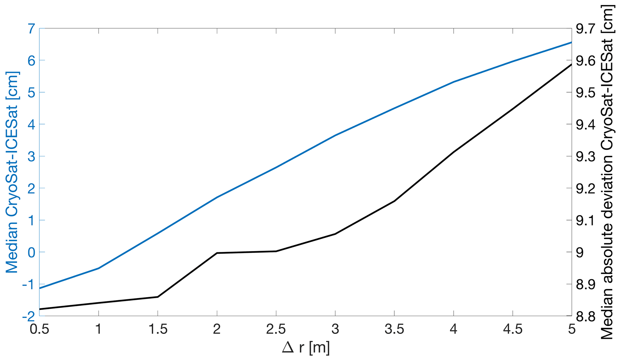
Figure 5Median (left axis) and median absolute deviation (right axis) of the height differences between CryoSat-2 and ICESat-2 (Δh calculated with Eq. 16) as a function of Δr. Outliers are removed using 10th and 90th percentiles.
However, it is not sufficient to conclude that LEPTA is robust to the choice of Δr by merely assessing Δh. The reason for this is that different Δr's might result in different horizontal locations, which are then compared to potentially different ICESat-2 measurements. Therefore, Fig. 6 shows the differences in the ellipsoidal height and horizontal position of the impact points obtained using Δr=2 m (Δr2) and Δr=1 m (Δr1). This comparison shows whether a Δr change of 1 m can result in large horizontal and vertical offsets. In the interior of the ice sheet this effect is small as the vertical and horizontal offsets resulting from Δr2 vs. Δr1 are close to 0. In the margin regions of LRM coverage, however, increasing Δr results in lower elevation of impact points and horizontal offsets with mean values up to 20 m and standard deviations up to 250 m.

Figure 6Mean and standard deviation of the differences between the height and horizontal location of the impact point obtained using Δr=2 m (Δr2) and Δr=1 m (Δr1). The mapped locations are based on the horizontal locations (x and y) derived from Δr1, tiled by the 25 km×25 km grid as in Fig. 4.
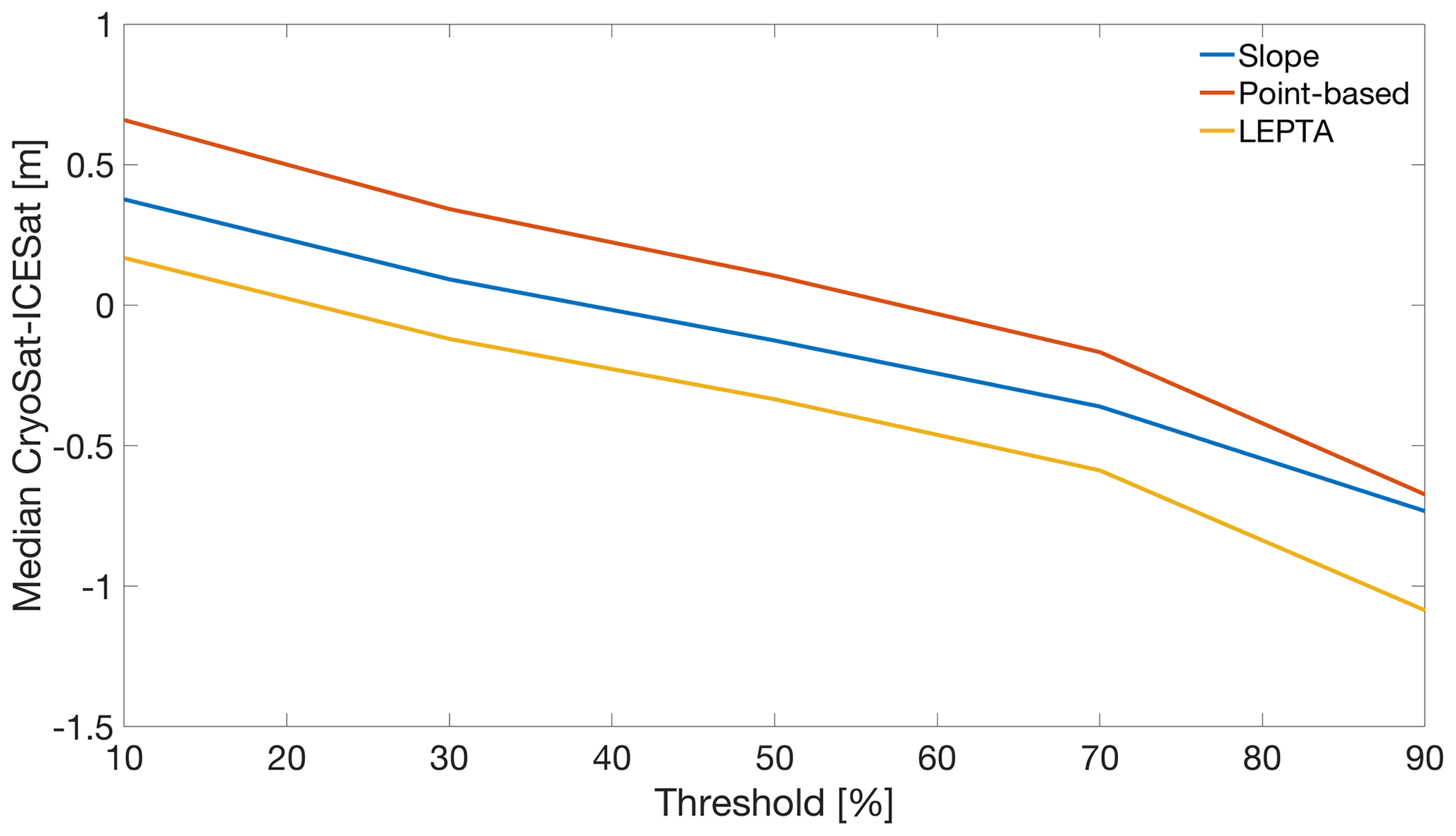
4.4 Assessment of OCOG retracker threshold dependence
Changing the OCOG retracker threshold from 10 % to 90 % results in retracked points further away from the satellite and hence lower height estimates (Fig. 7). For all methods, this behaviour is apparent as the median of Δh is reduced by approximately 1.2 m when the threshold increases from 10 % to 90 %. Changing the OCOG retracker threshold in LEPTA results only in a change in the height of Pl and does not affect the selection of the DEM points that contribute to Pl. This means that increasing the OCOG retracker threshold actually corresponds to increasing the depth of the radar return within the snowpack or firn. Moreover, Fig. 7 highlights that the adopted OCOG retracker threshold of 20 % for LEPTA results in a near-zero median difference compared to ICESat-2, indicating that on average it effectively detects the absolute ice-sheet height.
4.5 Sensitivity to potential biases in the DEM
To assess the sensitivity of the methods to potential constant ice-sheet elevation changes, we perform a sensitivity analysis in which we add biases to the DEM. Figure 8 shows that the slope and the point-based methods are not affected by these DEM biases, while they do affect LEPTA. The impact, though, depends on the sign of the bias. Adding a bias between −7.5 and −2.5 m (which corresponds to ice-sheet lowering) only changes the median Δh by approximately 2.3 cm, while adding a bias of 2.5 m (which corresponds to an increase in ice-sheet elevation) results in a median Δh that is 8.8 cm higher. A similar observation holds for the median absolute deviation of Δh. This dependency on the sign of the bias can be easily understood. The impact point is typically in the area where the range between the satellite and the terrain is smallest. Lowering the DEM and thereby increasing the range to the satellite hence result in a reduced number of DEM grid points within the search range (rend−rbegin). If no points are found, the search range is adjusted. Applying a positive bias, on the other hand, will result in other parts of the terrain being within the search range.
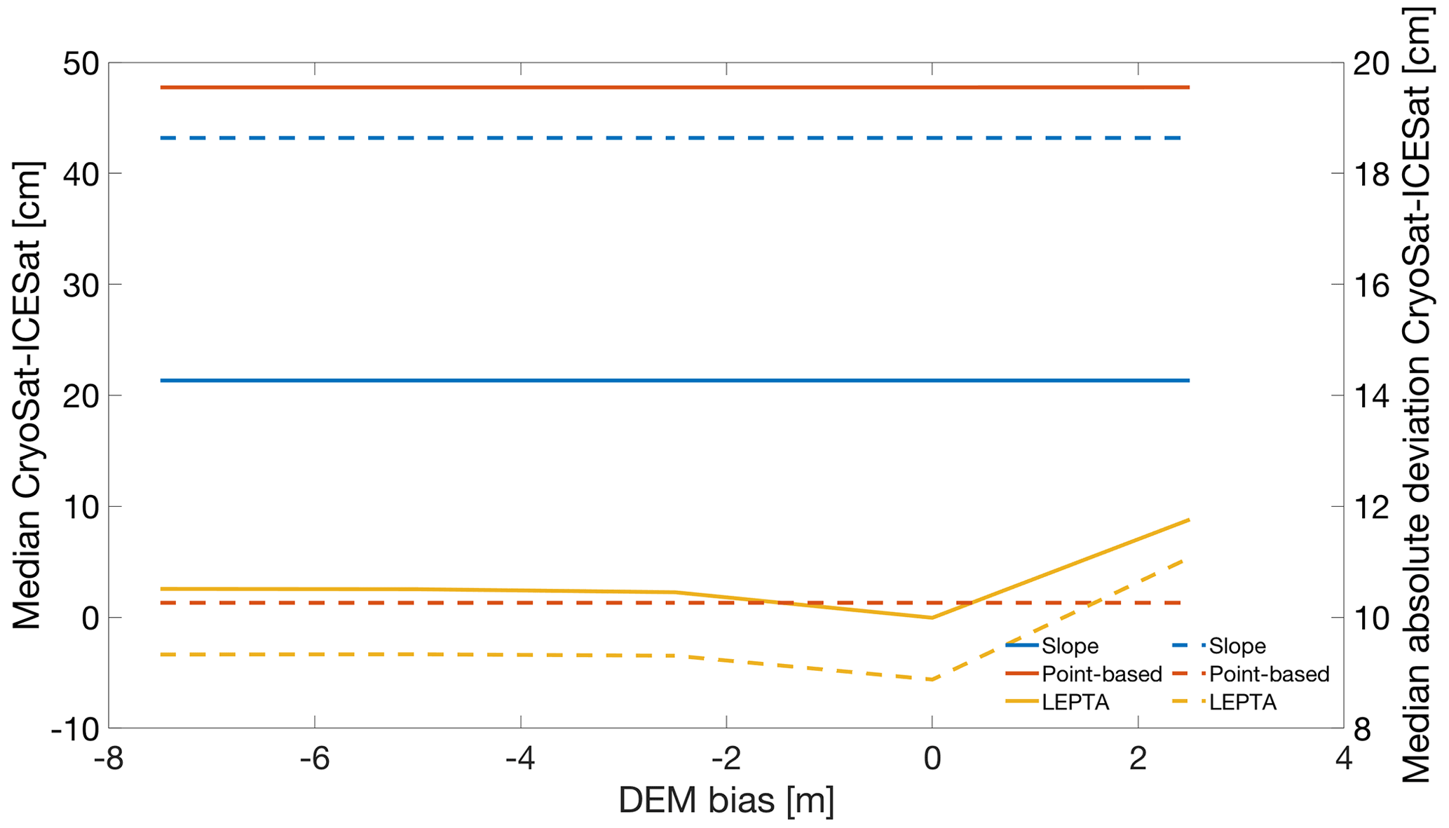
Figure 8Median (left axis, solid curves) and median absolute deviation (right axis, dashed curves) of height differences between CryoSat-2 and ICESat-2 (Δh calculated with Eq. 16) as a function of a bias in the DEM. Outliers are removed using 10th and 90th percentiles.
Despite LEPTA's sensitivity to a potential bias in the DEM, however, the median and median absolute deviation of Δh remain lower than the other methods for negative biases up to −7.5 m. With a positive bias of 2.5 m, the median absolute deviation of Δh from LEPTA is approximately 8 mm higher than that from the point-based method. In Appendix C, we present the results of a similar analysis to that shown in Fig. 6. This shows that the impact of a potential bias in the DEM is largest on the western side of the LRM zone, resulting in vertical and horizontal offsets with mean values of up to 2 and 50 m and standard deviations of up to 3.5 and 700 m, respectively.
4.6 Sensitivity to the resolution of the DEM
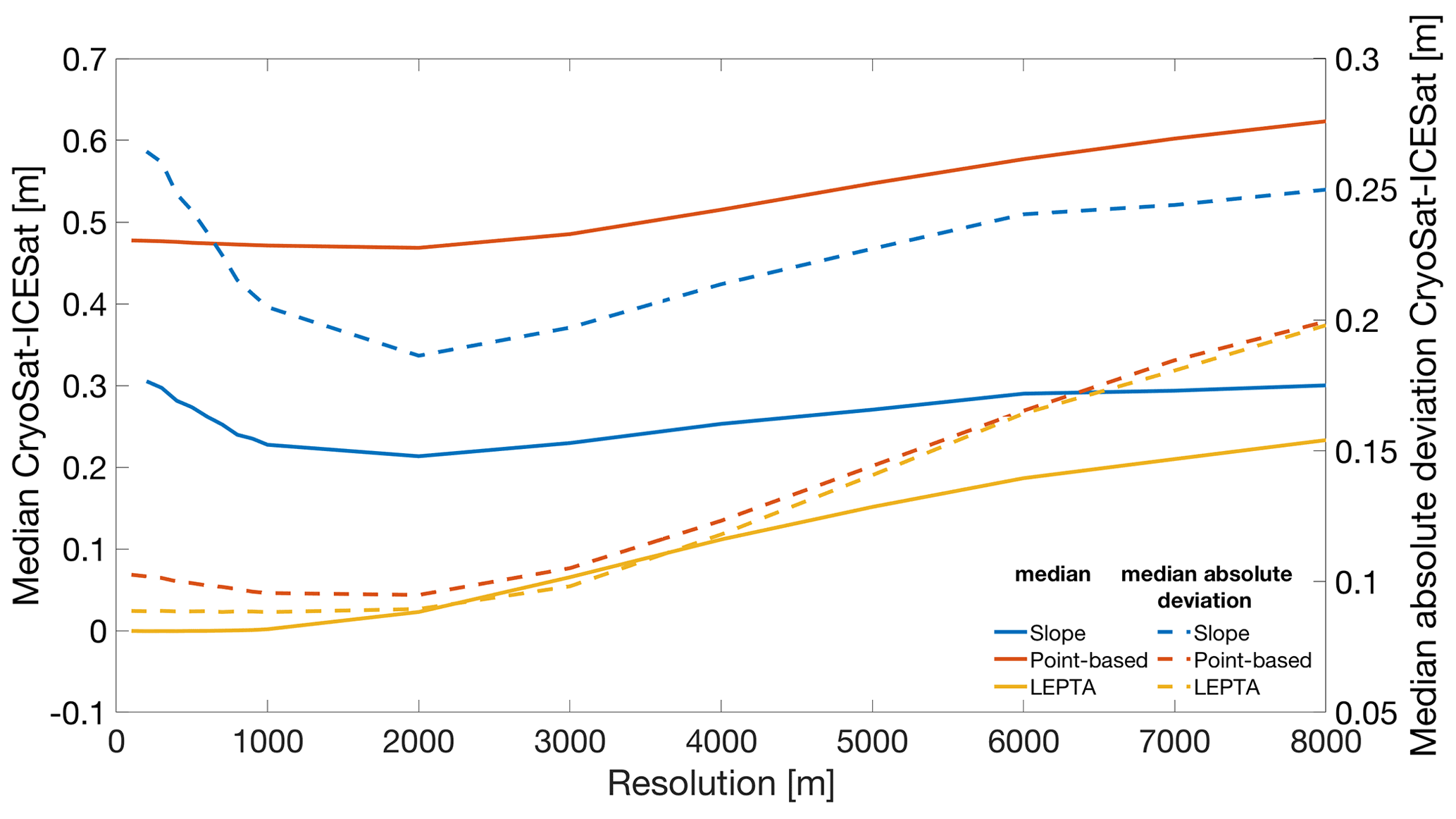
Figure 9 shows the effect of changing the DEM resolution on the median and median absolute deviation of Δh for different slope correction methods. For both the slope and the point-based method, the smallest median Δh is obtained at a 2 km resolution. For the slope method, the median Δh increases from 0.21 to 0.30 m when the DEM resolution increases from 2 to 8 km. For the point-based method, the variation in median Δh for DEM resolutions between 100 m and 2 km is within the millimetre level. Lowering the resolution down to 8 km increases the median to 0.62 m. For LEPTA, the variation in the median Δh for DEM resolutions between 100 m and 1 km is within the millimetre level. For lower resolutions, the median Δh increases to 0.23 m (8 km resolution). The smallest median absolute deviations for the slope method (0.19 m) and the point-based method (0.09 m) are obtained at a 2 km resolution. For LEPTA, the smallest median absolute deviation is obtained when using a 1 km resolution, though the values between resolutions of 100 m and 2 km vary at the millimetre level. For resolutions lower than 2 km, the median absolute deviation for both the point-based method and LEPTA increases by approximately 10 cm. For the slope method, the increase is 6 cm.
The comparison with ArcticDEM and validation based on ICESat-2 shows that the presented LEPTA method outperforms the slope and point-based methods as well as the ESA L2I product in accuracy with lower median, mean, and median absolute deviations. Especially in the margin regions of the LRM zone, heights derived from LEPTA correspond more closely to ICESat-2 height measurements compared to the slope method being used by ESA. This indicates that including leading edge information to determine the impact point results in an important improvement in the accuracy of CryoSat-2 LRM height estimations. By showing the importance of accurately determining the impact points over steeper margin areas, our results confirm earlier work of Levinsen et al. (2016) in the margin regions, where they also showed that the point-based method outperforms the slope method in median absolute deviation values. The improved performance of the point-based method and LEPTA method can be explained by the assumption of a constant slope within the footprint in the slope-based method, which results in a biased impact point further away from the satellite than the optimal location (Levinsen et al., 2016). An explanation for the improved performance of LEPTA over the point-based method can be found in the design of the method, which only takes into account areas that contribute to the rise of the CryoSat-2 LRM waveform leading edge (Fig. 1).
Our results also show that the ESA L2I product outperforms our self-implemented slope correction method. This agrees with Levinsen et al. (2016), who attributed the different performance between ESA's Envisat Radar Altimeter 2 products and their self-implementation of the slope correction method to the Doppler slope correction step implemented in ESA L2I products (Blarel and Legresy, 2012) and differences in the DEM used. We must admit that at this stage an explanation for the difference we obtained is lacking. Detailed analysis (not shown in this paper) shows that the differences cannot be explained by the fact that in our study we use another DEM.
The first sensitivity analysis shows that in terms of bulk statistics, LEPTA is quite robust to the definition of the search range. Compared to ICESat-2, the change in the median is <0.1 m for the interval over which we changed Δr, while the change in the median absolute deviation is at the millimetre level. Regionally, the impact may be larger. In particular, we observe changes of up to 1.46 m in the vertical and 231 m in the horizontal position of the impact points towards the margins of the LRM zone. In these areas, the mean and standard deviation of the leading edge width are larger. This, in turn, suggests using a larger Δr locally. The use of a spatially varying Δr is hence considered a potential further improvement of the method.
Increasing the OCOG retracker threshold lowers the height estimates for all methods. For both LEPTA and the point-based method, the horizontal position of the impact points does not change. This means that increasing the OCOG retracker threshold actually corresponds to increasing the depth of the radar return within the snowpack or firn. That is, the adopted threshold controls the observed penetration. Our results confirm that using a 20 % threshold gives on average comparable height estimates to ICESat-2. It is meanwhile worth noting that the probable scattering of ICESat-2 photons within the snowpack cannot be neglected (Smith et al., 2021).
Differently from the slope and point-based methods, LEPTA shows sensitivity to a bias in the DEM. The presence of a bias in the DEM does not affect the slope or the relative differences between the DEM points, which are key to the slope method and the point-based method, respectively. However, in the case of LEPTA, when the DEM heights are biased and the search range determined by the waveform leading edge is unchanged, the DEM points used to calculate the impact point of LEPTA are changed. According to Appendix C, this bias mainly affects the margins of the LRM coverage. Overall these bias effects indicate that it is key to have up-to-date, time-varying DEMs when applying LEPTA to correct for slope-induced errors. Changes in the elevation over time will affect the applied correction as well as the location of the impact point. However, in the case of non-homogeneous elevation changes (which will result in slope changes) this also holds for the other methods.
Sensitivity to DEM resolution shows that the slope and point-based methods perform best with an intermediate DEM resolution (2 km), which is consistent with Levinsen et al. (2016). However, differently from Levinsen et al. (2016), who obtained stable performance for the point-based method between a 2 and 4 km DEM resolution, our results show that the performance of the point-based method is stable when the DEM resolution is finer than 2 km. This can be attributed to differences in (i) the study area, (ii) the altimeter data used, (iii) the used DEM to compute the corrections, and (iv) the reference data and methods for validation. In principle, the point-based method should perform better with a finer DEM resolution because it has the advantage of using full topography rather than assuming a constant slope, as used by the slope method. While Levinsen et al. (2016) attributed the optimal 2 km resolution of other methods to the radar altimetry's ability to resolve small-scale surface features, our results show that Δr used by LEPTA to define the pulse-limited footprint may have a different impact (e.g. asymmetry around r20%). Therefore, for future studies, fine-tuning the impact of Δr is still of high importance.
Moreover, our experiment focuses on the performance of LEPTA in the CryoSat-2 LRM-covered regions over the Greenland ice sheet; therefore it remains to be studied how it performs over more complex terrains and Antarctica. Since the topography and DEM quality in other regions of the Earth are different from those in Greenland, we expect LEPTA to perform differently, and the impact of Δr can also vary. This phenomenon provides more aspects for future works.
Finally, while we use CryoSat-2 Baseline D data, Baseline E is available. However, we do not expect changes that significantly affect the conclusions of this study as the main changes in Baseline E are associated with the sea ice products (European Space Agency, 2021).
Reducing slope-induced errors is a key correction algorithm when processing LRM data over ice sheets. To correct for this error, different methods have been developed to determine the impact point, which all rely on footprint assumptions: e.g. the slope method, which assumes a constant slope within the footprint, or the point-based method, which assumes a fixed footprint size to determine the impact point by minimising the mean distance. Each of these methods has shortcomings as they neglect either the actual topography or the actual footprint that can be estimated by a combination of the leading edge and topography. To overcome these shortcomings, we present a leading edge point-based (LEPTA) method that corrects for the slope-induced error by including the leading edge information of the radar waveform to determine the impact point. The principle of the method is that only the points on the ground that are within the range determined by a specific search range that contributes to the rise of the waveform leading edge are used to determine the impact point.
Different methods for correcting the slope-induced errors are used in this study using CryoSat-2 measurements over the Greenland ice sheet. Statistics show that the LEPTA method outperforms all other methods with the smallest median and variability in errors. The median difference between ICESat-2 heights and CryoSat-2 heights derived by LEPTA using a 20 % OCOG threshold and Δr=1.25 m search range is 0.00 m. Spatially, LEPTA has a good improvement compared to the traditional slope method on the margins of the LRM-covered regions of the ice sheet as it derives heights generally more than 2 m closer to ICESat-2 measurements. LEPTA is sensitive to the definition of the search range and the bias in the DEM used to correct for the slope-induced error, mainly in the horizontal location of the impact points. However, comparison with ICESat-2 measurements generally shows centimetre-level sensitivity. Therefore, LEPTA is a method worth considering to obtain accurate height measurements with radar altimetry, especially in regions with complex topography.
ICESat-2 ATL06 Land Ice Height data include a large number of measurements between 1 January and 31 December 2019. Therefore, we compute the statistics of the differences between ICESat-2 heights (hICE2) and ArcticDEM interpolated to the corresponding locations (hDEMI) per beam pair. In this process, data outside the CryoSat-2 LRM zone have been excluded. The statistics are summarised in Table A1. All differences are computed as hICE2−hDEMI. The median difference between ICESat-2 and ArcticDEM for all beam pairs is 0.21 m, showing good agreement. The mean differences are around 5 cm.
Table A1Difference between ICESat-2 measurements and ArcticDEM values interpolated to ICESat-2 locations.
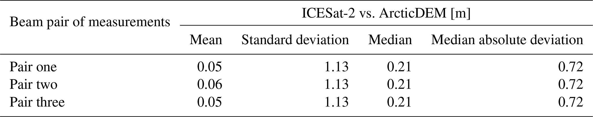
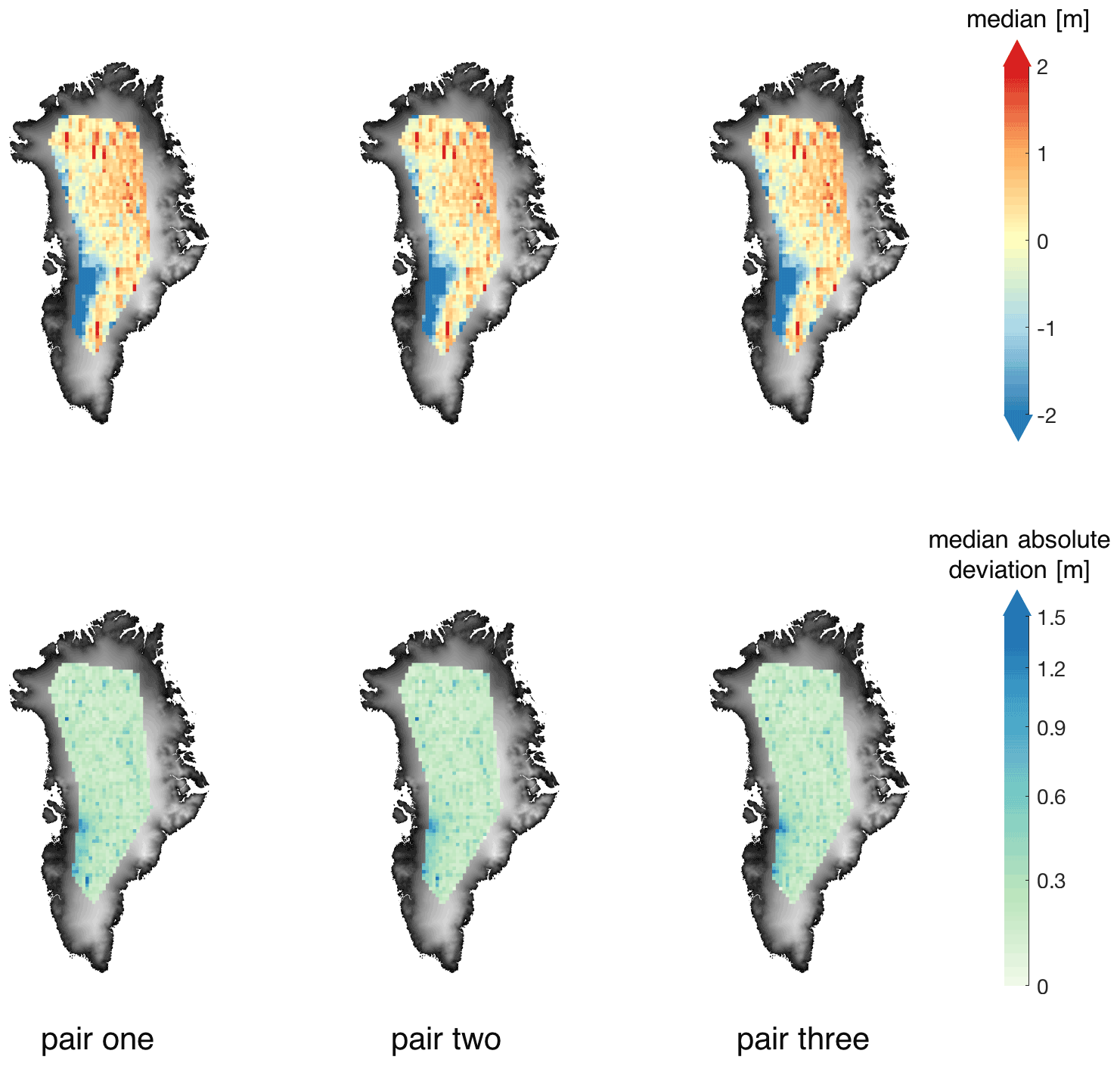
Figure A1Spatial distribution of median and median absolute deviation of the height difference between each pair of ICESat-2 beams and ArcticDEM (tiled in 25 km×25 km). The colours of the median absolute deviation plots are on a logarithmic scale.
Probability distribution functions of all methods are provided in Figs. B1 and B2 to illustrate the underlying skewness in Table 1 and Figs. 3 and 4 within the [−10 m, 10 m] range. However, the skewness can also be affected by large outliers, as also shown in the figures. For the slope method, the DEM resolution is 2 km. For LEPTA, Δr is 1.25 m. For the slope method, point-based method, and LEPTA, the retracker is the OCOG retracker with a 20 % threshold.

Figure B1Probability distribution functions of heights between CryoSat-2 and ArcticDEM derived from (a) ESA L2I, (b) the slope method, (c) the point-based method, and (d) LEPTA centred between −10 m and 10 m. To clearly show minimum and maximum values (values displayed with arrows), the curves are not displayed in the same panel.
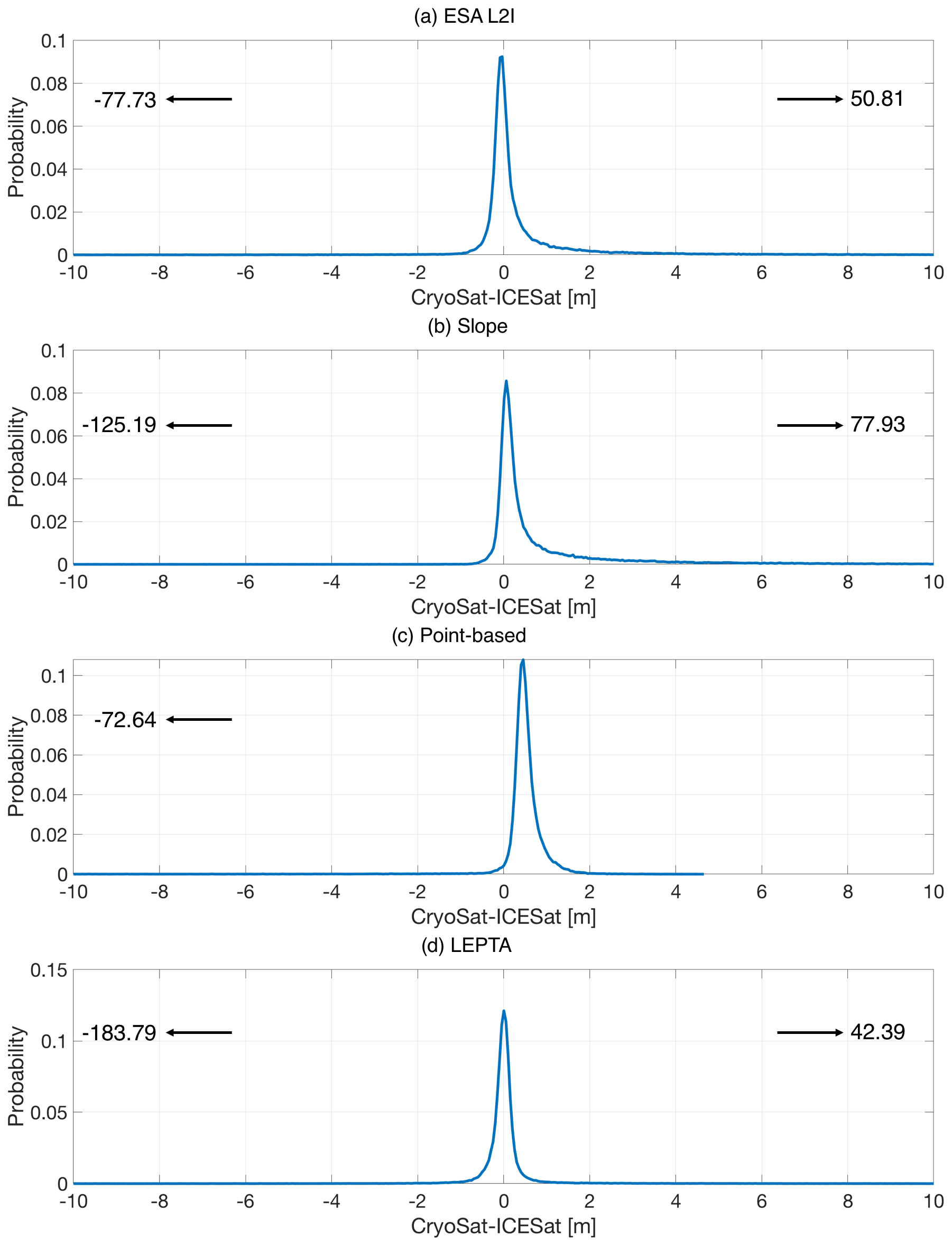
Figure B2Probability distribution functions of heights between CryoSat-2 and ICESat-2 derived from (a) ESA L2I, (b) the slope method, (c) the point-based method, and (d) LEPTA centred between −10 m and 10 m. To clearly show minimum and maximum values (values displayed with arrows), the curves are not displayed in the same panel.
Figures C1 and C2 show the three-dimensional difference between using the original ArcticDEM and the vertically displaced DEM to correct for the slope-induced error. The vertical and horizontal differences are calculated using the difference between the location of impact points Pl of the biased DEM minus the location of the impact points of the original ArcticDEM. Figure C1 shows that when the DEM used has a negative bias, the corrected heights are higher, the horizontal locations on the western side of the ice sheet are in general biased towards the northeast, and the horizontal locations on the northeast side of the ice sheet are biased towards the southwest. Figure C2 shows an inverse pattern when the DEM shows a positive bias. In the interior of the ice sheet, however, the effects of the DEM biases are small.
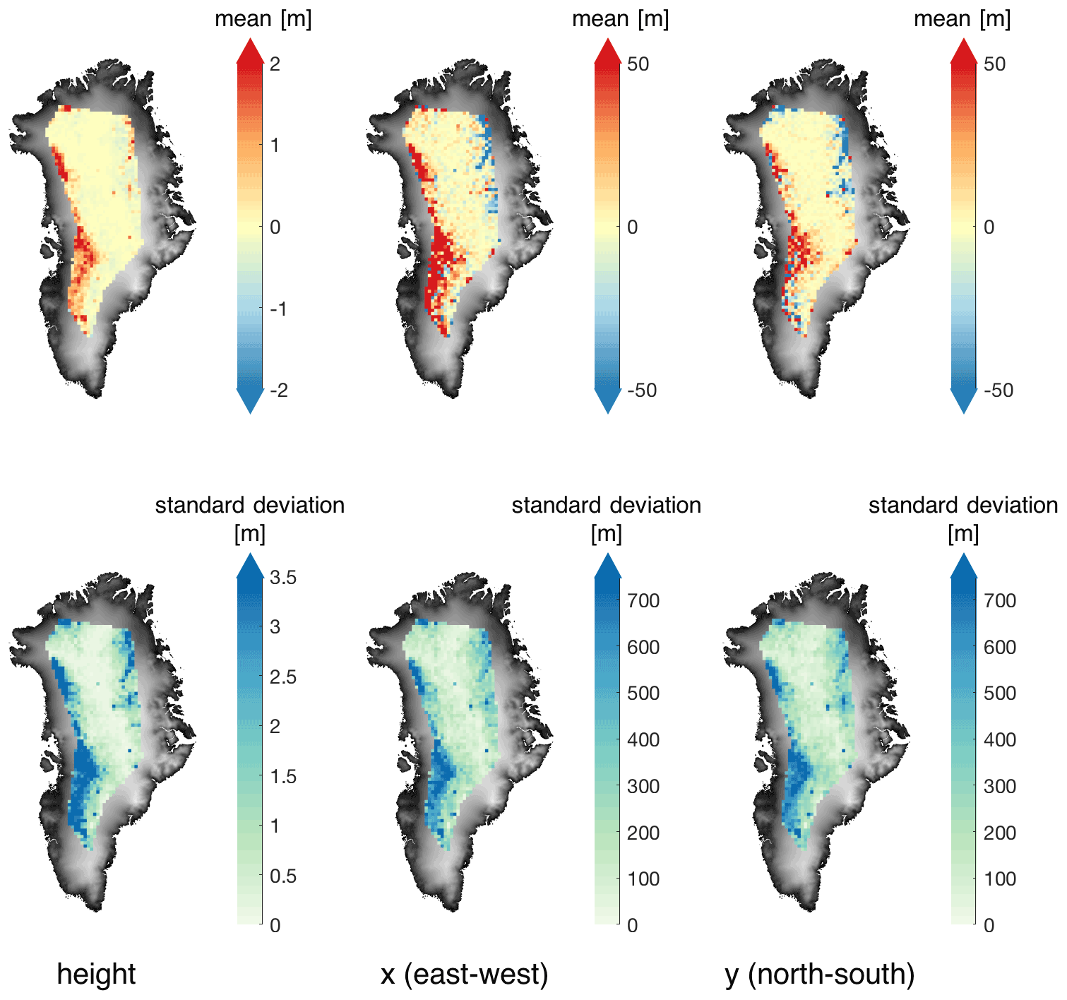
Figure C1Mean and standard deviation of vertical and horizontal difference in derived impact point Pl between (i) using the DEM with a homogeneous vertical displacement m (ΔhDEM1) and (ii) using the original ArcticDEM (DEMorig). The mapped locations are based on the horizontal locations (x and y) derived from DEMorig, tiled by the 25 km×25 km grid as in Fig. 6.
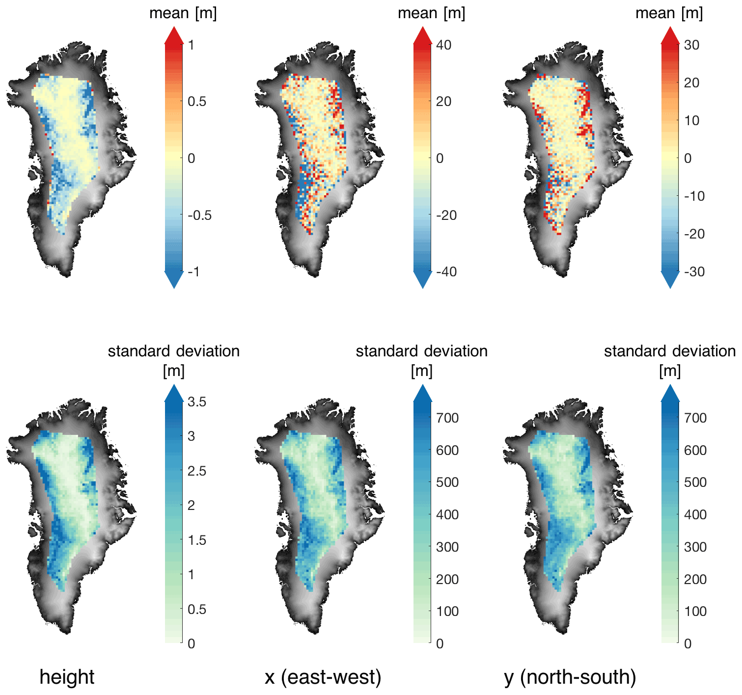
Figure C2Mean and standard deviation of vertical and horizontal difference in derived impact point Pl between (i) using the DEM with a homogeneous vertical displacement ΔhDEM=2.5 m (ΔhDEM1) and (ii) using the original ArcticDEM (DEMorig). The mapped locations are based on the horizontal locations (x and y) derived from DEMorig, tiled by the 25 km×25 km grid as in Fig. 6.
Software for the in-house processing of CryoSat-2 data from L1b to L2 is available on request from Cornelis Slobbe (d.c.slobbe@tudelft.nl).
The DEM of Greenland used for result visualisation is provided by Helm et al. (2014a, b; https://doi.org/10.1594/PANGAEA.831393) under a Creative Commons Attribution 3.0 Unported 20 licence. The CryoSat-2 L1b and L2I data are provided online by ESA, and the ICESat-2 L3A data are provided online by NSIDC (https://nsidc.org/data/atl06, last access: 3 July 2021).
WL conducted data management, processing, and analysis; produced the figures; and provided the manuscript with contributions from the other co-authors. CS designed the study and provided expertise and software for radar altimetry processing. SL provided support on statistical analysis and data visualisation.
At least one of the (co-)authors is a member of the editorial board of The Cryosphere. The peer-review process was guided by an independent editor, and the authors also have no other competing interests to declare.
Publisher's note: Copernicus Publications remains neutral with regard to jurisdictional claims in published maps and institutional affiliations.
ArcticDEM is provided by the Polar Geospatial Center under NSF OPP awards 1043681, 1559691, and 1542736. The DEM of Greenland used for result visualisation is provided by Helm et al. (2014a, b) under a Creative Commons Attribution 3.0 Unported licence. The CryoSat-2 L1b and L2I data are provided online by ESA, and the ICESat-2 L3A data are provided online by NSIDC (https://nsidc.org/data/atl06, last access: 3 July 2021).
The authors would also like to thank Roland Klees, Bert Wouters, Katarzyna Sejan, Jan Haacker, and Lorenzo Iannini for valuable discussions and Louise Sandberg Sørensen for the review and editing of this paper. Finally, we would like to thank the referees for reviewing and providing recommendations to improve this paper.
The research is supported by the Dutch Research Council (NWO) through the ALWGO.2017.033 project.
This paper was edited by Louise Sandberg Sørensen and reviewed by three anonymous referees.
Abdalati, W., Zwally, H. J., Bindschadler, R., Csatho, B., Farrell, S. L., Fricker, H. A., Harding, D., Kwok, R., Lefsky, M., Markus, T., Marshak, A., Neumann, T., Palm, S., Schutz, B., Smith, B., Spinhirne, J., and Webb, C.: The ICESat-2 laser altimetry mission, P. IEEE, 98, 735–751, https://doi.org/10.1109/jproc.2009.2034765, 2010. a
Adodo, F. I., Remy, F., and Picard, G.: Seasonal variations of the backscattering coefficient measured by radar altimeters over the Antarctic Ice Sheet, The Cryosphere, 12, 1767–1778, https://doi.org/10.5194/tc-12-1767-2018, 2018. a
Aublanc, J., Moreau, T., Thibaut, P., Boy, F., Rémy, F., and Picot, N.: Evaluation of SAR altimetry over the antarctic ice sheet from CryoSat-2 acquisitions, Adv. Space Res., 62, 1307–1323, https://doi.org/10.1016/j.asr.2018.06.043, 2018. a, b, c
Bamber, J. L.: Ice sheet altimeter processing scheme, Int. J. Remote Sens., 15, 925–938, https://doi.org/10.1080/01431169408954125, 1994. a, b, c, d, e, f
Blarel, F. and Legresy, B.: Investigations on the Envisat RA2 Doppler slope correction for ice sheets, in: European Space Agency-CNES Symp., 24–29 September 2012, Venice, Italy, edited by: Ouwehand, L., vol. 710, p.103, ISBN 978-92-9221-274-2, 2012. a
Bobach, T. A.: Natural Neighbor Interpolation – Critical Assessment and New Contributions, PhD thesis, Technische Universität Kaiserslautern, https://kluedo.ub.unikl.de/frontdoor/deliver/index/docId/2104/file/diss.bobach.natural.neighbor.20090615.pdf (last access: 9 June 2022), 2009. a
Brenner, A. C., Bindschadler, R. A., Thomas, R. H., and Zwally, H. J.: Slope-induced errors in radar altimetry over continental ice sheets, J. Geophys. Res., 88, 1617, https://doi.org/10.1029/jc088ic03p01617, 1983. a, b
Cooper, A.: Slope Correction By Relocation For Satellite Radar Altimetry, in: 12th Canadian Symposium on Remote Sensing Geoscience and Remote Sensing Symposium, IEEE, 10–14 July 1989, Vancouver, BC, Canada, https://doi.org/10.1109/igarss.1989.577978, 1989. a
Davis, C.: A robust threshold retracking algorithm for measuring ice-sheet surface elevation change from satellite radar altimeters, IEEE T. Geosci. Remote, 35, 974–979, https://doi.org/10.1109/36.602540, 1997. a, b, c, d, e
European Space Agency: L1b LRM Precise Orbit. Baseline D, https://doi.org/10.5270/CR2-cbow23i, 2019a. a
European Space Agency: L2 LRM Precise Orbit. Baseline D, https://doi.org/10.5270/CR2-k1o4pyh, 2019b. a
European Space Agency: New Ice Baseline E and Near Real Time Processors, https://earth.esa.int/eogateway/news/new-ice-baseline-e-and-near-real-time-processors (last access: 18 April 2022), 2021. a
Hai, G., Xie, H., Du, W., Xia, M., Tong, X., and Li, R.: Characterizing slope correction methods applied to satellite radar altimetry data: A case study around Dome Argus in East Antarctica, Adv. Space Res., 67, 2120–2139, https://doi.org/10.1016/j.asr.2021.01.016, 2021. a, b, c, d
Helm, V., Humbert, A., and Miller, H.: Elevation and elevation change of Greenland and Antarctica derived from CryoSat-2, The Cryosphere, 8, 1539–1559, https://doi.org/10.5194/tc-8-1539-2014, 2014a. a, b, c, d, e, f
Helm, V., Humbert, A., and Miller, H.: Elevation Model of Greenland derived from CryoSat-2 in the period 2011 to 2013, links to DEM and uncertainty map as GeoTIFF, Pangaea [data set], https://doi.org/10.1594/PANGAEA.831393, 2014b. a, b, c, d
Howat, I. M., Porter, C., Smith, B. E., Noh, M.-J., and Morin, P.: The Reference Elevation Model of Antarctica, The Cryosphere, 13, 665–674, https://doi.org/10.5194/tc-13-665-2019, 2019. a
Hurkmans, R. T. W. L., Bamber, J. L., and Griggs, J. A.: Brief communication “Importance of slope-induced error correction in volume change estimates from radar altimetry”, The Cryosphere, 6, 447–451, https://doi.org/10.5194/tc-6-447-2012, 2012. a
Lacroix, P., Dechambre, M., Legrésy, B., Blarel, F., and Rémy, F.: On the use of the dual-frequency ENVISAT altimeter to determine snowpack properties of the Antarctic ice sheet, Remote Sens. Environ., 112, 1712–1729, https://doi.org/10.1016/j.rse.2007.08.022, 2008. a
Levinsen, J. F., Simonsen, S. B., Sorensen, L. S., and Forsberg, R.: The Impact of DEM Resolution on Relocating Radar Altimetry Data Over Ice Sheets, IEEE J. Sel. Top. Appl., 9, 3158–3163, https://doi.org/10.1109/jstars.2016.2587684, 2016. a, b, c, d, e, f, g, h, i, j, k, l
Meloni, M., Bouffard, J., Parrinello, T., Dawson, G., Garnier, F., Helm, V., Di Bella, A., Hendricks, S., Ricker, R., Webb, E., Wright, B., Nielsen, K., Lee, S., Passaro, M., Scagliola, M., Simonsen, S. B., Sandberg Sørensen, L., Brockley, D., Baker, S., Fleury, S., Bamber, J., Maestri, L., Skourup, H., Forsberg, R., and Mizzi, L.: CryoSat Ice Baseline-D validation and evolutions, The Cryosphere, 14, 1889–1907, https://doi.org/10.5194/tc-14-1889-2020, 2020. a
National Snow and Ice Data Center (NSIDC): ATL06 release 005 known issues, https://nsidc.org/sites/nsidc.org/files/technical-references/ICESat2_ATL06_Known_Issues_v005.pdf (last access: 18 April 2022), 2021. a
Noh, M.-J. and Howat, I. M.: Automated stereo-photogrammetric DEM generation at high latitudes: Surface Extraction with TIN-based Search-space Minimization (SETSM) validation and demonstration over glaciated regions, GISci. Remote Sens., 52, 198–217, https://doi.org/10.1080/15481603.2015.1008621, 2015. a
Noh, M.-J. and Howat, I. M.: The Surface Extraction from TIN based Search-space Minimization (SETSM) algorithm, ISPRS J. Photogramm., 129, 55–76, https://doi.org/10.1016/j.isprsjprs.2017.04.019, 2017. a
Porter, C., Morin, P., Howat, I., Noh, M.-J., Bates, B., Peterman, K., Keesey, S., Schlenk, M., Gardiner, J., Tomko, K., Willis, M., Kelleher, C., Cloutier, M., Husby, E., Foga, S., Nakamura, H., Platson, M., Wethington Jr., M., Williamson, C., Bauer, G., Enos, J., Arnold, G., Kramer, W., Becker, P., Doshi, A., D'Souza, C., Cummens, P., Laurier, F., and Bojesen, M.: ArcticDEM, Harvard Dataverse, https://doi.org/10.7910/DVN/OHHUKH, 2018. a
Remy, F., Mazzega, P., Houry, S., Brossier, C., and Minster, J.: Mapping of the Topography of Continental Ice by Inversion of Satellite-altimeter Data, J. Glaciol., 35, 98–107, https://doi.org/10.3189/002214389793701419, 1989. a
Roemer, S., Legrésy, B., Horwath, M., and Dietrich, R.: Refined analysis of radar altimetry data applied to the region of the subglacial Lake Vostok/Antarctica, Remote Sens. Environ., 106, 269–284, https://doi.org/10.1016/j.rse.2006.02.026, 2007. a, b, c, d, e, f, g, h, i
Schröder, L., Horwath, M., Dietrich, R., Helm, V., van den Broeke, M. R., and Ligtenberg, S. R. M.: Four decades of Antarctic surface elevation changes from multi-mission satellite altimetry, The Cryosphere, 13, 427–449, https://doi.org/10.5194/tc-13-427-2019, 2019. a
Slater, T., Shepherd, A., McMillan, M., Muir, A., Gilbert, L., Hogg, A. E., Konrad, H., and Parrinello, T.: A new digital elevation model of Antarctica derived from CryoSat-2 altimetry, The Cryosphere, 12, 1551–1562, https://doi.org/10.5194/tc-12-1551-2018, 2018. a
Smith, B., Fricker, H. A., Holschuh, N., Gardner, A. S., Adusumilli, S., Brunt, K. M., Csatho, B., Harbeck, K., Huth, A., Neumann, T., Nilsson, J., and Siegfried, M. R.: Land ice height-retrieval algorithm for NASA's ICESat-2 photon-counting laser altimeter, Remote Sens. Environ., 233, 111352, https://doi.org/10.1016/j.rse.2019.111352, 2019. a
Smith, B., Fricker, H. A., Gardner, A., Siegfried, M. R., Adusumilli, S., Csathó, B. M., Holschuh, N., Nilsson, J., Paolo, F. S., and the ICESat-2 Science Team: ATLAS/ICESat-2 L3A Land Ice Height, Version 4, National Snow and Ice Data Center (NSIDC), https://doi.org/10.5067/ATLAS/ATL06.004, 2020a. a
Smith, B., Hancock, D., Harbeck, K., Roberts, L., Neumann, T., Brunt, K., Fricker, H., Gardner, A., Siegfried, M., Adusumilli, S., Csathó, B., Holschuh, N., Nilsson, J., and Paolo, F.: Algorithm Theoretical Basis Document (ATBD) for Land Ice Along-Track Height Product (ATL06), Tech. rep., ICESat-2 Project Science Office, https://nsidc.org/sites/nsidc.org/files/technical-references/ICESat2_ATL06_ATBD_r004.pdf (last access: 9 June 2022), 2020b. a
Smith, B., Hancock, D., Harbeck, K., Roberts, L., Neumann, T., Brunt, K., Fricker, H., Gardner, A., Siegfried, M., Adusumilli, S., Csathó, B., Holschuh, N., Nilsson, J., and Paolo, F.: ICESat-2 Algorithm Theoretical Basis Document for Land Ice Height (ATL06) Release 005, https://nsidc.org/sites/nsidc.org/files/technical-references/ICESat2_ATL06_ATBD_r005.pdf (last access: 18 April 2022), 2021. a
Wingham, D. J., Rapley, C. G., and Griffiths, H.: New Techniques in Satellite Altimeter Tracking Systems, in: Digest – International Geoscience and Remote Sensing Symposium (IGARSS), 8–11 September 1986, vol. ESA SP-254, Zurich, 1339–1344, https://www.researchgate.net/publication/269518510_New_Techniques_in_Satellite_Altimeter_Tracking_Systems (last access: 9 June 2022), 1986. a
- Abstract
- Introduction
- Data and pre-processing
- Methods
- Results
- Discussion
- Conclusions
- Appendix A: Comparison between ICESat-2 measurements and ArcticDEM
- Appendix B: Probability distribution functions of the height differences showing skewness
- Appendix C: Impact of a bias in the ArcticDEM on the 3D location of the LEPTA impact points
- Code availability
- Data availability
- Author contributions
- Competing interests
- Disclaimer
- Acknowledgements
- Financial support
- Review statement
- References