A probabilistic seabed–ice keel interaction model

Landfast ice is a common coastal feature in the Arctic Ocean and around the Antarctic continent. One contributing and stabilizing mechanism is the grounding of sea ice ridges in shallow water. Recently, a grounding scheme representing this effect on sea ice dynamics was developed in order to improve the simulation of landfast ice by continuum-based sea ice models. This parameterization assumes that the ridged keel thickness is proportional to the mean thickness. Results demonstrated that this simple parameterization notably improves the simulation of landfast ice in many regions such as in the East Siberian Sea, the Laptev Sea and along the Alaskan coast. Nevertheless, a weakness of this approach is that it is based solely on the mean properties of sea ice. Here, we extend the parameterization by taking into account subgrid-scale ice thickness distribution and bathymetry distribution, which are generally non-normal, and by computing the maximum seabed stress as a joint probability interaction between the sea ice and the seabed. The probabilistic approach shows a reasonably good agreement with observations and with the previously proposed grounding scheme while potentially offering more physical insights into the formation of landfast ice.

1 Introduction

Landfast ice is sea ice that remains immobile despite external forces acting on it. It occurs because of two different processes. One is when sea ice is constrained by the land boundaries, i.e. when it is thick and solid enough that it resists compressive, tensile and shear stresses arising from integrated external forces. In narrow channels of the Canadian Arctic Archipelago (CAA), in fjords or in between nearby islands, landfast ice occurs because the tensile strength of the ice everywhere in between land masses, including at the wall boundaries, is sufficient to resist along-channel wind and current forces. This mechanism has been identified as the main cause for landfast ice in the Kara Sea (Olason, 2016), Nares Strait between Greenland and Canada (Dumont et al., 2009; Plante et al., 2020), or the CAA (Lemieux et al., 2016) using sea ice models having either a viscous-plastic or elasto-brittle rheology. Note that this phenomenon can also be simulated using discrete element models with friction and cohesion in between particles (e.g. Garcimartín et al., 2010).

The second distinctive process is in open coastal regions where sea ice is attached to the land on one side but has a free edge adjacent to the ocean. In order to maintain the stability of landfast ice covers extending over large distances from the coast, the horizontal cohesive strength of sea ice is not sufficient. It must be grounded; i.e. some of the deformed and thicker sea ice present in the ice cover must reach down to the seabed in order to provide the required additional resisting force. When sea ice ridges act as anchor points, the seaward landfast ice edge can reach the 20–30 m isobath (Mahoney et al., 2007). In some regions (e.g. East Antarctica), anchor points can also be provided by grounded icebergs. This can bring the seaward landfast ice edge over deeper water with icebergs often grounded in 400–500 m depths (Van Achter et al., 2022).

More often than not, the two processes are intertwined, as once an anchor point through grounding is in place, some of the internal horizontal stress is redirected there. The most striking examples of this are the extensive landfast ice that forms off the northern coast of Siberia, in the Laptev and East Siberian seas (Yu et al., 2014), and along the Alaskan coast, in the Beaufort Sea (Mahoney et al., 2007, 2014).

Various attempts at representing landfast ice in Arctic simulations have been conducted in the past with a mix of these processes, starting from the crude zero velocity condition using an ice thickness-to-depth ratio of Lieser (2004), an increased maximum viscosity in Olason (2016), an artificially large tensile strength in Itkin et al. (2015) or the seabed stress parameterization of Lemieux et al. (2015, hereafter referred to as L15).

Focusing on the latter – and some adaptations in Lemieux et al. (2016) for the Arakawa B grid staggering – L15 have developed a parameterization for estimating the seabed stress due to grounded ridges¹. It estimates the thickness of the largest ridges within a model grid cell as a linear function of the mean thickness, which will be referred to in the following as the LKD (linear keel depth) parameterization. When the mean thickness is greater than a critical value that is a function of the local water depth, the parameterization assumes that ridge keels that are deep enough to reach the sea floor exist. In such a case, a non-zero seabed stress is added to the sea ice momentum equation. The maximum seabed stress that can be supported by the grounded ridge is a function of the weight of the ridge in excess of hydrostatic balance. This parameterization has the practical advantage of being simple and easy to add in single- and multi-category sea ice models. Moreover, model simulations run over a pan-Arctic domain with that parameterization show that seabed–ice interactions lead to realistic landfast ice covers along the Alaskan and Siberian coasts (L15; Lemieux et al., 2016).

However, as recognized by L15, there are a few caveats to that model. The first one is that it assumes that ridges thicker than the mean ice thickness exist, irrespective of the ice formation and deformation history. This is of course not physically adequate as there are situations where the ice thickness mostly results from thermal growth and much less from mechanical deformation. This is particularly true for landfast ice. For example, in a situation where newly formed ice becomes landfast as it consolidates in relatively shallow waters, the mean thickness will mainly increase due to freezing at the base, or snow conversion to ice at the top. As sea ice remains immobile, no ridges are formed. However in this specific case, the parameterization assumes that ridge keels always exist, which can lead to an overestimation of the seabed–ice interaction. Despite the fact that the LKD parameterization can be tuned with observations of landfast ice in terms of extent and timing, the predictive capability of such a model is thus questionable in a context of rapid climate changes that affect ice thickness, ice types and ice dynamics.

The second caveat of the LKD parameterization is that the keel depth varies linearly with the mean ice thickness, with a tunable proportionality constant approximately equal to 8. However, many observational studies show that the thickness of the deepest keels depend nonlinearly on the mean thickness. For example, Melling and Riedel (1996) report observations of ice draft in the Beaufort Sea that suggest a power-law dependence of the keel draft on the surrounding level ice thickness with an exponent of 0.5. Using submarine sonar observations in Davis Strait, Wadhams et al. (1985) show that the ice thickness distribution of ice thicker than 3–4 m follows a negative exponential. More recently, Haas et al. (2010) presented results from a 2400 km long pan-Arctic airborne survey over old ice in the Arctic Ocean, between Svalbard and Alaska, and confirmed that the ice thickness distribution is generally skewed with an exponential tail for values larger than 3–4 m. Positively skewed ice thickness distributions mean that extreme values are not proportional to the mean, but rather non-linearly correlated to it.

Most contemporary sea ice models use an ice thickness distribution (ITD) to parameterize thermal processes and to describe the subgrid-scale thickness variability arising from deformations. Flato and Hibler (1995) explored in detail how different parameterizations of mechanical redistribution in a 28-category model influence the resulting ITD in various places of the Arctic Ocean. The model confirmed that positive skewness of the ITD is ubiquitous. However, the ITD is not typically resolved with such a large number of categories in climate models or short-term forecasting systems (5–10 categories are usually the norm). Thus, the tail of the distribution is still poorly represented in models. Nonetheless, we can analytically approximate the form of the tail and provide a parameterization that more faithfully represents the thickest keels and their interactions with the seabed.

The main objective of this paper is to layout a probabilistic representation of the seabed–ice interaction that takes advantage of the evolutive ITD. It can also take advantage of the high-resolution bathymetric information that is typically lost when a model bathymetry is processed and filtered for a particular configuration. The work of Adcroft (2013) is a good example where subgrid-scale bathymetry information is used to better represent the flow over a nonuniform seabed. Parameterizations of seabed–ice interactions that rely on good-quality bathymetric data are in principle less dependent on empirical tuning compared to parameterizations that ignore subgrid-scale information.

The structure of the paper is as follows. Section 2 presents a derivation of the probabilistic seabed–ice stress, and Sect. 3 describes the numerical implementation and experiments. Results are presented in Sect. 4 and discussed in Sect. 5.

2 The probabilistic approach

The sea ice thickness field is highly heterogeneous due to mechanical processes such as compressive ridging that thickens the ice and crack opening that creates ice-free areas in which new ice can form. Since the pioneering work of Thorndike et al. (1975), these processes are explicitly represented in sea ice numerical models through the evolution of an ice thickness distribution (ITD) usually called g(h), where h is the ice thickness. As noted by Thorndike et al. (1975), g(h) can be interpreted as a probability density function (PDF) that gives the likelihood that a point will have a thickness h. In this sense, the ice thickness is interpreted as a random variable x, which has a PDF g(x) that is supposed to be representative of the ice thickness distribution over of certain area – corresponding to the grid cell area in the context of a numerical model. In the rest of the paper, we will use the symbol h when we refer to statistical moments of the distribution. As we are interested to know if and how sea ice interacts with the seabed, we will assume that the seabed depth in a given grid cell is also represented by a random variable y characterized by the probability density function b(y). Ice of thickness x touches the seabed if the draft of the ice, which is function of ice thickness that we call D(x), is larger than the height of the water column y.

Generally, D(x) represents the hydrostatic equilibrium of the floating ice under snow loading. However in the following, we will discard the snow contribution and consider the simpler relationship $D\left(x\right)={\mathit{\rho }}_{\mathrm{i}}x/{\mathit{\rho }}_{\mathrm{w}}$, where ρ_i and ρ_w are the ice and water densities, respectively. This relationship is easily invertible and allows simplification of the equations.

Assuming that both variables are independent, the probability that the ice is in contact with the seabed is noted as 𝒫(D(x)>y) and is obtained by

$$\begin{array}{}\text{(1)}& \mathcal{P}\left(D\left(x\right)>y\right)=\underset{\mathrm{0}}{\overset{\mathrm{\infty }}{\int }}\underset{\mathrm{0}}{\overset{y=D\left(x\right)}{\int }}g\left(x\right)b\left(y\right)\mathrm{d}y\mathrm{d}x.\end{array}$$

If we assume that g(x) and b(y) represent respectively the ITD and the water column height distribution over a surface area S, then S𝒫(D(x)>y) represents the total area of ice that is in contact with the seabed and that can potentially exert friction inside the surface S. Now the maximum frictional stress of a flat block of ice of thickness x sitting on the ocean floor at a depth y is equal to μ_sF_N(x,y), where μ_s is a static friction coefficient and F_N(x,y) is the normal force exerted by the excess weight of the ice sitting on the ocean floor, normalized over a unit surface area of 1 m². Neglecting once again the effect of snow, this force is expressed as

$$\begin{array}{}\text{(2)}& F_{\mathrm{N}}(x,y)=\widehat{g}\left({\mathit{\rho }}_{\mathrm{i}}x-{\mathit{\rho }}_{\mathrm{w}}y\right),\end{array}$$

where $\widehat{g}$ is the gravitational acceleration. Considering that x and y are fully characterized by their respective probability density functions, the total maximum friction stress is obtained by integrating μ_sF_N(x,y) over all water depth lower than D(x) and over all thickness values, yielding

$$\begin{array}{}\text{(3)}& {\mathit{\tau }}_{\mathrm{b}}^{max}={\mathit{\mu }}_{\mathrm{s}}\widehat{g}\underset{\mathrm{0}}{\overset{\mathrm{\infty }}{\int }}\underset{\mathrm{0}}{\overset{y=D\left(x\right)}{\int }}\left({\mathit{\rho }}_{\mathrm{i}}x-{\mathit{\rho }}_{\mathrm{w}}y\right)g\left(x\right)b\left(y\right)\mathrm{d}y\mathrm{d}x.\end{array}$$

This expression differs from the one proposed by L15 (their Eq. 21) in two ways. First, the LKD parameterization prescribes one keel depth for each mean thickness value, while in the probabilistic formulation, the solution is degenerated, which means that there can be multiple keel depth values associated with different ITDs that have the same mean thickness value. The second difference is that the keel depth values depend non-linearly on the mean thickness, as opposed to LKD where the prescribed dependence is linear. This will be further illustrated in Sect. 3.1 when discussing the ITD.

To facilitate the numerical implementation, we follow L15 and the instantaneous horizontal seabed–ice stress vector τ_b is written as a function of the sea ice velocity $\mathit{u}=u\widehat{\mathit{ı}}+v\widehat{\mathit{j}}$ as

$$\begin{array}{}\text{(4)}& {\mathit{\tau }}_{\mathrm{b}}=-{\mathit{\tau }}_{\mathrm{b}}^{max}\left({\displaystyle \frac{u\widehat{\mathit{ı}}+v\widehat{\mathit{j}}}{\left|\mathit{u}\right|+u_{\mathrm{0}}}}\right)e^{-{\mathit{\alpha }}_{\mathrm{b}}(\mathrm{1}-A)},\end{array}$$

where α_b is a constant controlling the dependence of the seabed stress on the ice concentration A, and u₀ is a small velocity scale that assures a smooth transition between static and dynamic regimes. As in L15, it is also assumed that the kinetic friction coefficient is equal to the static one (i.e. μ_s). The seabed stress vector is then included in the momentum equation as

$$\begin{array}{}\text{(5)}& m_{\mathrm{i}}{\displaystyle \frac{D\mathit{u}}{Dt}}=-\mathit{k}\times m_{\mathrm{i}}f\mathit{u}+{\mathit{\tau }}_{\mathrm{a}}+{\mathit{\tau }}_{\mathrm{w}}+{\mathit{\tau }}_{\mathrm{b}}+\mathrm{\nabla }\cdot {\mathit{\sigma }}_{\mathrm{i}}-m_{\mathrm{i}}\widehat{g}\mathrm{\nabla }\mathit{\eta },\end{array}$$

where τ_a is the wind stress, τ_w is the water stress, f is the Coriolis parameter, m_i is the combined mass of ice and snow per unit surface, σ_i is the internal stress tensor of the ice (here due to the viscous-plastic rheology, following an elliptic yield curve) and η is the sea surface elevation. In the next section, we describe how Eq. (3) is computed, and we emphasize these differences by comparing the results using LKD as well as observations.

3 Probability density distributions and numerical implementation

Solving for the seabed stress using the probabilistic approach presented in the previous section requires that distributions are known. In principle, these can have arbitrary shapes if the integral of Eq. (3) is computed numerically, which is done here (see Sect. 3.2). The following subsections describe the ProbSI model and how it is implemented. We present how distributions of ice thickness, or ice draft, and bathymetry are determined, how their parameters are optimized to represent seabed–ice interactions, and how sensitive the resulting seabed stress is to these parameters.

3.1 Ice thickness distribution

The number of thickness categories sea ice models typically use is a trade-off between the representativity of ice dynamics and thermodynamics and computational cost. Sea ice components of Earth climate modelling systems typically use five categories, which is the default number of the Los Alamos Community Ice (CICE) model (Hunke et al., 2021). The Canadian Regional Ice-Ocean Prediction System (RIOPS, described in Dupont et al., 2015; Smith et al., 2021) uses 10 categories. In all cases, thickness categories are chosen to represent the positively skewed distributions. However, their number is generally too low to resolve the exponentially decreasing tail of the distribution, and thus to make a precise assessment of the deepest keels that are the most likely to interact with the seabed. Figure 1a shows an example of an ITD discretized as in RIOPS with 10 categories with levels at 0, 0.1, 0.15, 0.3, 0.5, 0.7, 1.2, 2.0, 4.0 and 6.0 m. All categories are populated with ice. The last category includes ice thicker than 6.0 m and is in theory unbounded (note that the upper bound is arbitrarily set at 10 m in the plot). In CICE, the mean thickness inside each category is, in practical terms, defined as the ratio between the partial ice volume divided by the partial concentration of a particular populated category. This thickness varies between the bounds of the category following thermodynamic processes, advection and mechanical ridging. However, ice properties can be redistributed in thickness space out of a given category to adjacent ones regardless of the relative position of this mean category thickness inside the bounds. The actual PDF of ice thickness inside each category is approximated by a delta function, a uniform distribution or a decreasing exponential depending on the user's input, and sometimes on the considered process (as shown below).

Figure 1 Examples showing how the maximum seabed stress due to seabed–ice friction is calculated. Panels (a, c, e) show an example where all ice thickness categories are populated, including the last one (yellow bin) – note that for visualization purposes the last category is bounded arbitrarily at 10 m. The corresponding thickest keel draft is the 99.7th percentile of the thickness PDF (black line), which is x₉₉₇=11.73 m (open triangle). Panels (b, d, f) show an example where the partial concentration of the thickest ice category is zero. The corresponding thickest keel draft is the maximum thickness of the last category (black triangle, x=6 m), even though x₉₉₇=9.96 m (open triangle). The maximum basal stress ${\mathit{\tau }}_{\mathrm{b}}^{max}$ is here computed with a Gaussian bathymetric PDF with μ_b=10.5 m and σ_b=1.0 m² and truncated at 3σ_b on both sides of the distribution (blue line). The PDFs are shown in linear (e, f) and logarithmic scales (c, d).

In order to represent the tail of the distribution and the depth of the largest keels, we proceed in two steps. The first step consists in computing the mean and variance of the discretized (model) ITD and finding a positively skewed PDF – let us call it f(x) – that has the same mean and variance. This ensures that the PDF conserves the same total concentration and mean ice thickness. The second step consists in identifying the percentile that best represents the thickness of the deepest keel for this PDF and then truncating the PDF to that value. This is necessary because PDFs are usually defined from 0 to infinity, and because the contribution of small probabilities for extreme values is amplified by the term (ρ_ix−ρ_wy) in Eq. (3), which may result in an overestimation of the seabed stress. Note that the truncation to a certain percentile does not conserve the total integrated concentration or the volume. In the following, we will provide some estimation of this error.

There is no general consensus on the functional form that the ITD should follow, and no model exactly reproduces observed ITDs. Wadhams et al. (1985) suggested that ice thicker than 2–4 m can often be fitted by a negative exponential, while Flato and Hibler (1995) used a power law. Toppaladoddi and Wettlaufer (2015) assumed that ridged ice formation follows a random process that is similar to the Brownian motion that obeys an advection-diffusion Fokker–Planck equation for which the solution has a negative exponential. Roberts et al. (2019), using variational principles, macroporosity and a Mohr–Coulomb ridging rheology, show results that slowly converge to a negative exponential. However, despite the lack of consensus on the functional form, the positive skewness is generally accepted as a property that a representative ITD should have.

The function we use here is the log-normal distribution that is both representative of observed ITDs with negative exponential tails and easily manipulable numerically. It is given by

$$\begin{array}{}\text{(6)}& f_{\mathcal{L}\mathcal{N}}\left(x^{\prime }\right)={\displaystyle \frac{\mathrm{1}}{\sqrt{\mathrm{2}\mathit{\pi }}\mathit{\sigma }{x}^{\prime }}}\exp \left({\displaystyle \frac{(\ln x^{\prime }-\mathit{\mu }{)}^{\mathrm{2}}}{\mathrm{2}{\mathit{\sigma }}^{\mathrm{2}}}}\right),\end{array}$$

where μ and σ are determined from the mean m and variance v by the following expressions

$$\begin{array}{}\text{(7)}& {\displaystyle }\mathit{\mu }=\ln \left({\displaystyle \frac{m^{\prime }}{\sqrt{\mathrm{1}+v^{\prime }/m^{\prime \mathrm{2}}}}}\right),\text{(8)}& {\displaystyle }\mathit{\sigma }=\sqrt{\ln (\mathrm{1}+v^{\prime }/m^{\prime \mathrm{2}})}.\end{array}$$

In this context, x^′ is an adimensional quantity that is defined as $x^{\prime }=x/\mathit{\lambda }$, where x is the dimensional thickness (e.g. in metres) and λ is the unit thickness (e.g. 1 m) that can be chosen arbitrarily. The same applies to $m^{\prime }=m/\mathit{\lambda }$ and $v^{\prime }=v/{\mathit{\lambda }}^{\mathrm{2}}$ in Eqs. (7) and (8), which are similarly adimensionalized. To ease the interpretation of the results in the remainder of the paper, we use the dimensional quantities in metres, i.e. with λ=1 m. The dimensional percentile value $x_{\mathrm{p}}=\mathit{\lambda }{x}_{\mathrm{p}}^{\prime }$, corresponding to the value below which a proportion p of thickness values fall, is given by

$$\begin{array}{}\text{(9)}& x_{\mathrm{p}}=\mathit{\lambda }\exp \left[\mathit{\mu }+\sqrt{\mathrm{2}{\mathit{\sigma }}^{\mathrm{2}}}{\text{erf}}^{-\mathrm{1}}\left(\mathrm{2}p-\mathrm{1}\right)\right].\end{array}$$

The value of x_p should represent the thickness of the deepest keel one can find in an ice cover characterized by the corresponding ITD and is a parameter to which the seabed stress parameterization is very sensitive. How this value is tuned is presented in Sect. 3.3.1. Once x_p is determined, f_ℒ𝒩(x) is truncated so that values x>x_p do not contribute to the integral of Eq. (3). Hence, the error introduced in truncating the integral using p=0.997 is 0.3 % in terms of concentration, which is by definition equal to 1−p. The mean thickness of the truncated ITD in Fig. 1c is equal to 2.13 m, which corresponds to a 2 % difference compared to the full distribution. These errors decrease in course with increasing values of p.

Figure 1b shows a second example of an ITD where all categories are populated except the very last one, shown in yellow in Fig. 1a. In this case, the redistribution scheme of the model did not produce ice thicker than 6 m (the maximum value of the ninth category). Consequently, the log-normal PDF associated with that ITD is truncated at 6 m (black triangle in Fig. 1b, f).

3.2 Bathymetry distribution

The bathymetry field of coupled ice–ocean numerical models is typically built from gridded datasets such as GEBCO (Becker et al., 2009) or ETOPO (Amante and Eakins, 2009), which are themselves aggregations of data acquired from many different sources. In some places, the density of data points is much higher than the model grid resolution, while in some sparse areas, data are absent and some level of interpolation is required. The method proposed here would allow for taking into account the subgrid-scale distribution of the bathymetric field. However, instead of creating these distributions at a particular resolution and from a given database, we assume that the distribution is Gaussian everywhere, characterized by a mean value μ_b and a standard deviation σ_b. We then carry out a sensitivity analysis of the simulated landfast ice cover on the spread value and the impact of truncating the distribution. This way, the model we propose here could be applicable in a variety of configurations where the subgrid depth information is not necessarily available, given however that the spread value is optimized. As mentioned above, the integration of Eq. (3) is done numerically, by sampling the two distributions over 100 points and integrating over the appropriate bounds.

3.3 Parameter optimization

As L15 showed in their sensitivity study, the occurrence of landfast ice does not depend to a first order on the magnitude of the maximum seabed–ice stress, which scales with the friction coefficient μ_s, but rather on the keel thickness that determines when the ice is touching the seabed (i.e. the probability of contact). In the probabilistic parameterization presented here, the probability of contact in an oceanic cell is mainly controlled by x_p, which is the maximum value of g(x), and on the shallowest value of the bathymetry distribution b(y).

3.3.1 Deepest keel estimation

Using upward-looking sonar moored in the Beaufort Sea, Melling and Riedel (1996) measured the ice draft over 941 km of drifting sea ice during winter 1991–1992. They related the draft of the keels h_dk to the draft of surrounding level ice h_dl. The scatter plot relating these two quantities (Fig. 13 of Melling and Riedel, 1996) is a cloud of points for which the upper bound follows $h_{\mathrm{dk}}=\mathrm{16}\sqrt{h_{\mathrm{dl}}}$. Unsurprisingly, there is no unique relationship between the thickness of a keel and the thickness of the surrounding level ice. Amundrud et al. (2004) used a similar methodology using another upward-looking sonar dataset, also in the Beaufort Sea, and found a similar relationship with an upper bound that follows $h_{\mathrm{dk}}=\mathrm{20}\sqrt{h_{\mathrm{dl}}}$ (Fig. 13 of Amundrud et al., 2004).

Ideally, a sea ice model that represents ridging dynamics (keel formation) should reproduce the broad characteristics of the observed relationship. The recent work of Roberts et al. (2019) represents a comprehensive effort to improve how Earth system models reproduce ridge statistics. They do so by revisiting the energy-based method of Rothrock (1975) using variational principles and by taking into account sea ice macroporosity through a bivariate distribution. However, in order to be generally applicable, the seabed stress formulation introduced here relies solely on the ITD. To retrieve the thickness of the deepest keels in a PDF, here using a log-normal distribution, we assume that it corresponds to a percentile that would best fit the observations.

Comparing model estimations of the thickest keels to direct field observations such as those presented by Melling and Riedel (1996) and Amundrud et al. (2004) requires deriving a proxy for level ice thickness using only the available 10-category ITD of the model. It is not possible to isolate individual ridges from the model ITD and associate their thickness with the thickness of level ice flanking them, as is done by Melling and Riedel (1996). Instead, if we assume that ice thicker than a certain value h_r was only formed through ridging, we can discriminate ridged ice and consider that the level ice thickness is the mean thickness of ice thinner than h_r. Choosing h_r=4 m seems reasonable considering that values observed by Amundrud et al. (2004) reach up to 3.5 m. We thus define h_level as the mean thickness of the ice thinner than 4 m. Figure 2a shows that h_level is a scattered function of h_mean, with values unsurprisingly lying below the 1:1 curve that saturate around 3.5 m. Figure 2c shows that x₉₉₇, i.e. the 99.7th percentile value of the log-normal fit of the ITD, is a good predictor of the largest keel depth when compared to empirical relations of Amundrud et al. (2004) and Melling and Riedel (1996). The relation between x₉₉₇ and h_level bears a similar meaning as in Melling and Riedel (1996), especially in very compact conditions, where other mechanical and thermal effects happening in marginal ice zones and in polynyas are avoided, a subset that is highlighted by the black dots. Note there that model quantities are thicknesses, while observations are ice draft. Despite this discrepancy and the proxy definition we use for level ice, it is quite stunning to see how the shape of the point cloud is similar to what is observed in the field. This illustrates the major innovation of the probabilistic nonlinear approach compared to previous deterministic and linear approaches. The choice of the percentile value has been done so that most of the point cloud lies below the empirical curves, but the definitive tuning procedure is done by comparing the simulated landfast ice area with observations (this is discussed in Sect. 4). In the following and otherwise noted, x₉₉₇ will be used to truncate f_ℒ𝒩(x).

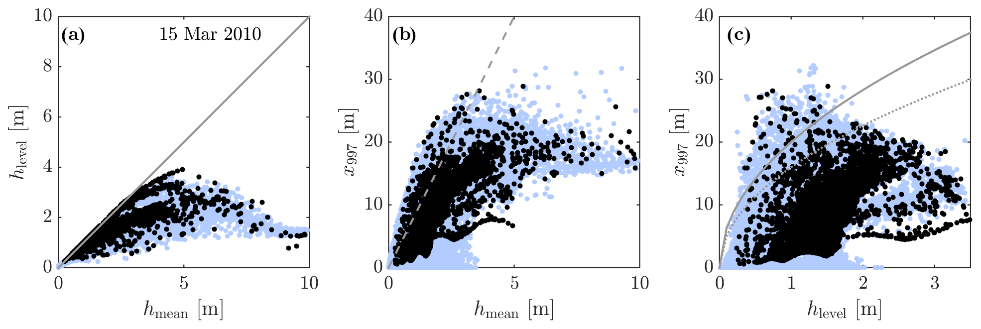
Figure 2 (a) Relationships between level ice thickness h_level, defined as the mean thickness of ice thinner than 4 m, and mean ice thickness h_mean. The full line indicates a 1:1 ratio. (b) The largest keel thickness x₉₉₇ as a function of the mean ice thickness h_mean. The grey dashed line represents the LKD parameterization. (c) x₉₉₇ as a function of h_level, with the solid and dashed lines showing the empirical relationship of Melling and Riedel (1996) and Amundrud et al. (2004), respectively. Blue dots represent all grid points for 15 March 2010 while black dots show a subset with A>0.99999.

3.3.2 Seabed stress sensitivity

Figure 1c and d show different f_ℒ𝒩(x) based respectively on the ITD of Fig. 1a and b, interacting with a truncated Gaussian PDF at ±3σ_b for the bathymetry. In panel c, the thickness PDF is truncated at x₉₉₇=11.73 m, which allows for interactions with the bathymetry, and in panel d x₉₉₇=9.96 m lies outside the PDF space, the maximum thickness being limited to the last bounded and populated category of the ITD. This is an illustration of the sensitivity of the seabed stress on the ITD, which is zero when no overlap exists between the two distributions.

The effect of the standard deviation and truncation of the bathymetric PDF on the seabed stress is further investigated and compared to the LKD method. Full Gaussian (FG), truncated Gaussian (at ±3σ_b; TG) and truncated uniform (covering the same span as the truncated Gaussian; TU) PDFs are tested with two different values of the standard deviation. Figure 3a shows that, for σ_b=1.0 m and low values of the mean water depth μ_b, the new seabed stress magnitude is higher than that of LKD and that this relation reverses at higher values of μ_b. Note that the figure uses a logarithmic scale and that differences are a few orders of magnitude. As expected, TG yields a lower stress than that of FG when the ice is nearly touching the seabed, but both curves converge as the water depth decreases. The truncated uniform distribution (TU) yields stress values that are slightly larger as the probability of shallow bathymetry intersecting ice is always higher. Increasing the standard deviation of the water depth distribution (Fig. 3b) also increases the probability of shallow bathymetry intersecting ice and therefore leads to a slight increase in stress. For the same reason, the stress approaches zero at a greater mean water depth for all bathymetry PDFs. Because of the two latter effects, the stress for the PDFs crosses over that of LKD at higher values of μ_b. The cutoff values for both truncated PDFs are the same and nearly equal to x₉₉₇+3σ_b, i.e. when there is no longer any contact. For σ_b=1.0 m, the cutoff happens at a value below 14.73 m, and for σ_b=2.5 m, the cutoff happens at a value below 19.23 m. The cutoff for LKD happens at ${\mathit{\mu }}_{\mathrm{b}}=k_{\mathrm{1}}{h}_{\mathrm{mean}}=\mathrm{16.36}$ m, which is qualitatively very close to that of the truncated PDFs for σ_b=2.5 m. As it was already noted that the actual value of the maximum seabed stress has less impact than the value of the deepest keels, the cutoff value is therefore interesting evidence that, at σ_b=2.5 m, LKD and TG formulations should yield similar results. On the other hand, FG cutoff would be too low at σ_b=1.0 m and too large at 2.5 m with a slow sloping off. In this context, we found the behaviour of TG more similar to that of LKD and therefore more appropriate for a numerical implementation. We show further down how the landfast area is impacted by the choice of the standard deviation in the bathymetry distribution using TG.

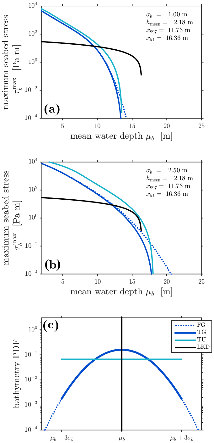
Figure 3 Maximum seabed stress ${\mathit{\tau }}_{\mathrm{b}}^{max}$ computed with Eq. (3) using the ice thickness distribution of Fig. 1a, fitted with a lognormal distribution with mean m=2.18 m and variance v=3.03 m², truncated at x₉₉₇=11.73 m, as a function of the mean water depth μ_b with standard deviation σ_b=1.0 m (a) and σ_b=2.5 m (b), on a logarithmic scale. The friction coefficient is set to μ_s=0.7. The three bathymetry probability density functions (PDFs) are shown in (c): a full Gaussian distribution (FG, dashed blue), a truncated Gaussian distribution (TG, blue) and a uniform distribution (TU, blue-green) both truncated at ±3σ_b. The LKD method with k₁=7.5 and k₂=15 N m⁻³ is represented in black, and, since it is independent of σ_b, its bathymetry distribution is a Dirac delta function (e.g. the vertical line in c).

3.4 Experimental setup

A coupled ice–ocean model is used to perform the numerical experiments. The model grid covers the Arctic and part of the North Atlantic oceans with a nominal 0.25^∘ resolution. This grid represents a subdomain of the 0.25^∘ global ORCA grid, which has a grid spacing of ∼12 km in the central Arctic.

The sea ice model is the Community Ice Model CICE version 5.0 (Hunke et al., 2015) with some modifications: the UK Met Office CICE-NEMO interface (Megann et al., 2014), the grounding parameterization of L15 and Lemieux et al. (2016), and the new seabed stress parameterization described in this paper. NEMO version 3.6 (Madec, 2008) is the ocean model. It is applied in a variable volume and nonlinear free surface configuration with 75 vertical levels, which closely follows that of Lemieux et al. (2016). The turbulent kinetic energy scheme (TKE, a simple one-equation closure) is used for ocean mixing. Both sea ice and ocean models use an advective time step of 10 min (600 s). The EVP method with 480 subcycles is used to solve the sea ice momentum equation. Ten (10) thickness categories (as defined above and used first in Smith et al., 2016) are employed for the CICE ice thickness distribution (ITD) model.

Vertical profiles of temperature, salinity and ocean currents are prescribed at the North Atlantic and North Pacific open boundaries. These profiles come from GLORYS2 version 4 reanalysis (Garric et al., 2017) monthly-averaged fields. Atmospheric forcing fields for the coupled ice–ocean simulations are the 33 km resolution reforecasts of Smith et al. (2014). This atmospheric dataset covers the period 2001–2010. This is a relatively short period for conducting a spinup followed by an analysis of model results. As done in Lemieux et al. (2018) and explained below, this issue is mitigated by using a special procedure for the spinup.

Average (September–October 2001) sea ice concentration from the National Snow and Ice Data Center (NSIDC, http://nsidc.org/data/seaice_index/, last access: 30 November 2010) and average (October–November 2003) sea ice thickness field derived from ICESat data (https://nsidc.org/data/icesat, last access: 7 November 2010) were used to initialize the sea ice model. The sea ice starts at rest. For the ocean model, the initial temperature and salinity fields are September–October averages from WOA13_95A4 (Locarnini et al., 2013; Zweng et al., 2013). The ocean also starts at rest; the currents and the sea surface height field are set to zero.

These fields were used to initialize the CICE-NEMO model for what we refer to as the pseudo-spinup. The pseudo-spinup consists in a simulation running from 1 October 2001 to 30 September 2002 that is repeated three times. Following these 3 years of simulation, the coupled model is restarted on 1 October 2001 and run until 15 September 2004. These last 3 years of the simulation are considered the final spinup. Note that the LKD parameterization was used for the complete spinup procedure. September 2004 simulated fields are used to restart simulations for optimizing parameters (see Sect. 4) and to perform long-term experiments for model result analyses.

All the simulations for this paper use the ice strength parameterization of Hibler (1979) with $P^{*}=\mathrm{27.5}$ N m⁻². The ellipse aspect ratio is e=1.4, and a small tensile strength value is added by setting k_t=0.05 (Lemieux et al., 2016). Following Chikhar et al. (2019). The ice–atmosphere roughness and ice–ocean roughness are respectively set to $\mathrm{5.7}\times {\mathrm{10}}^{-\mathrm{4}}$ and $\mathrm{1.82}\times {\mathrm{10}}^{-\mathrm{2}}$ m. The other sea ice physical parameters are the default values of CICE version 5.0 (Hunke et al., 2015).

From the September 2004 simulated fields, two simulations are restarted and run until 31 December 2010. In the first simulation, the LKD is used while in the second simulation the new probabilistic seabed–ice stress approach is used (referred to as ProbSI). Outputs from the numerical experiments are daily mean values defined at tracer points. The daily mean ice velocity ${\mathit{u}}_{\mathrm{d}}=u_{\mathrm{d}}\widehat{\mathit{ı}}+v_{\mathrm{d}}\widehat{\mathit{j}}$ is used to calculate the ice speed $(u_{\mathrm{d}}^{\mathrm{2}}+v_{\mathrm{d}}^{\mathrm{2}}{)}^{\mathrm{1}/\mathrm{2}}$ at each grid cell. As in L15 and Lemieux et al. (2016), ice is assumed to be landfast if its 2-week mean speed is lower than $\mathrm{5}\times {\mathrm{10}}^{-\mathrm{4}}$ m s⁻¹. A 2-week window is used as a shorter period could cause false assessments of landfast ice when the winds are weak. The landfast ice area for a given region (the East Siberian, Laptev and Kara seas, the three regions under consideration, are displayed in Fig. 4) is computed every 2 weeks by summing the area of landfast cells. Using the McGill sea ice model, L15 found an optimal value of k₁=8 for the LKD method. A similar optimization procedure (results not shown) was repeated with our CICE-NEMO setup and led to a close value of k₁=7.5. Finally, in ProbSI, a maximum water depth is used for limiting the seabed–ice keel interaction to waters shallower than 50 m.

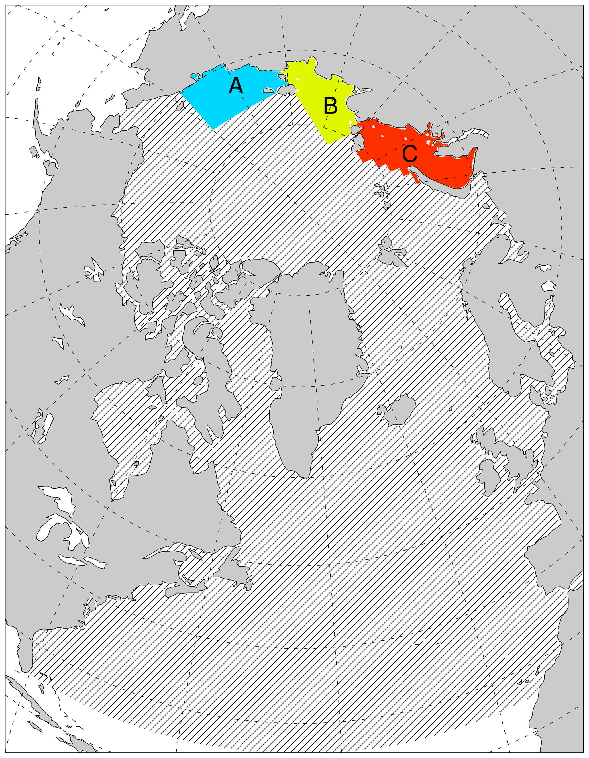
Figure 4 Computational domain shown in slanted black lines along with the three regions for which total landfast area is calculated (“A” for East Siberian Sea, “B” for Laptev Sea and “C” for Kara Sea). Taken from Fig. 2 of Lemieux et al. (2016), © Crown copyright 2016.

3.5 Landfast ice dataset

In order to determine which model formulation is the most appropriate, we compare the landfast ice area to that derived from observations, here taken as analyzed ice charts. The US National Ice Center (USNIC) Arctic Sea Ice Charts and Climatologies in Gridded Format dataset covers the period from 1972 through 2007 (Fetterer and Fowler, 2006). The analysis of landfast ice is derived from the US National Ice Center weekly/bi-weekly ice charts (Detrick et al., 2001) (https://usicecenter.gov/Products/ArcticData, last access: 7 February 2021). This product is analyzed by subject matter experts using near-real-time satellite data and various additional meteorological and oceanographic data resources and provides observed sea ice concentration, stage of development and partial concentration of sea ice types. Using the same approach, the landfast ice dataset is extended to cover our period of interest. We refer to our extension of the NIC dataset as NICext. Landfast ice is identified where the form of ice is coded as “08”. Occasionally, landfast ice is reported with a total concentration of $\mathrm{10}/\mathrm{10}$ without any information about partial concentration, stage of development or form of ice. The ice charts are composed of polygons of various sizes and shapes. Within a polygon, it is assumed that the ice condition is homogeneous. To make use of the information, the ice charts are first rasterized on a 5 km grid. Then to compare with the model on the model grid, the nearest grid point on the 5 km grid is taken. The difference between the two landfast ice datasets (NIC and NICext) is in general very minor during the overlapping period as can be seen in Fig. 8.

4 Results

Figure 5 shows a pan-Arctic view of the daily averaged mean thickness h_mean, the keel depth given by x₉₉₇ in ProbSI and x_k1=k₁ h_mean in LKD, as well as the difference between the two on 15 April 2010. Clearly, LKD overestimates the keel depth almost everywhere compared to x₉₉₇. The largest difference occurs north of the CAA where the keel depth reaches values larger than 35 m. Even though such keel depth values have been observed on certain occasions, they still remain extremely rare, and it is clearly unrealistic to have them covering such a large area (e.g. Wadhams and Davy, 1986). In the Lincoln Sea, north of the Nares Strait that separates Canada and Greenland at 83^∘ N, the difference between x_k1 and x₉₉₇ is larger than 20 m, owing to the fact that the ice there is thick (h_mean≃6 m) but relatively undeformed compared to sea ice in nearby ridging lines. This stems again from the linear dependence between x_k1 and h_mean, which overestimates the keel depth for mean thickness over 4 m (Fig. 2). The only locations where x_k1 is smaller than x₉₉₇ are in marginal ice zones and leads, where ice is generally thinner. Note that these differences between LKD and ProbSI do not have any impacts except in regions where there is grounding. Over the Siberian shelves, where grounding is prevalent, x_k1 is moderately larger than the probabilistic estimation.

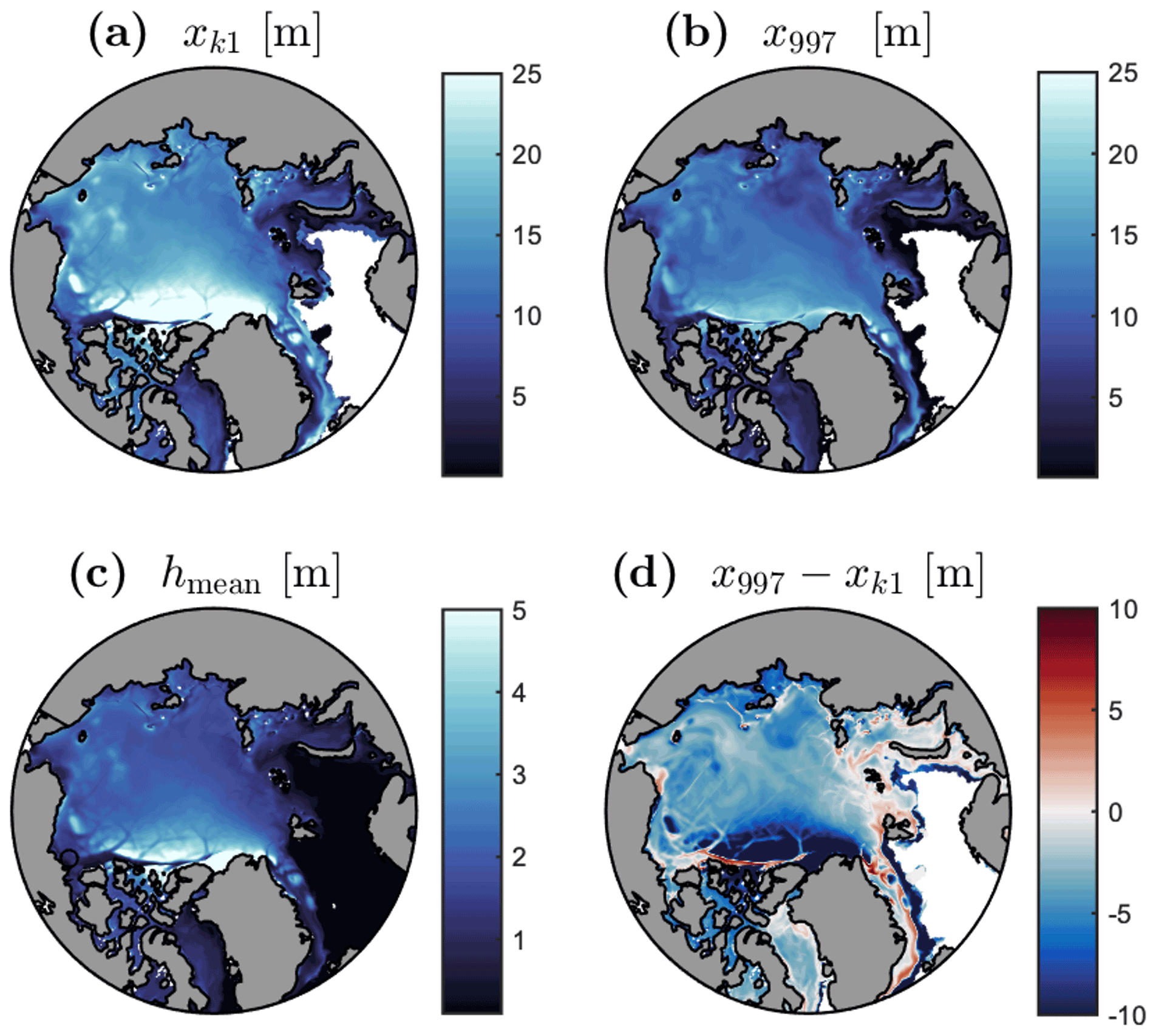
Figure 5 Ridge keel thickness estimated by the LKD parameterization x_k1=7.5h_mean (a) and by x₉₉₇ (b), the mean ice thickness h_mean (c), and the difference between x₉₉₇ and x_k1 (d) on 15 April 2010.

Figure 6a shows the weak sensitivity of running the model with the probabilistic approach and different values of the cutoff percentile at σ_b=0.5 m in terms of the area covered with landfast ice in Region B (Laptev Sea). There are even periods where the order is not necessarily the expected one as the second lowest cutoff percentile can result in the largest area (e.g. beginning of April 2005). The sensitivity to the variance of the water depth distribution is also explored in Fig. 6b with x₉₉₇. The results closer to the observations for the maximum landfast ice cover are visually in between σ_b= 1.5 and 3.5 m. An in-between value of 2.5 is therefore chosen hereafter when not specified. This also corroborates the initial findings of the sensitivity analyses presented in Sect. 3.3.2.

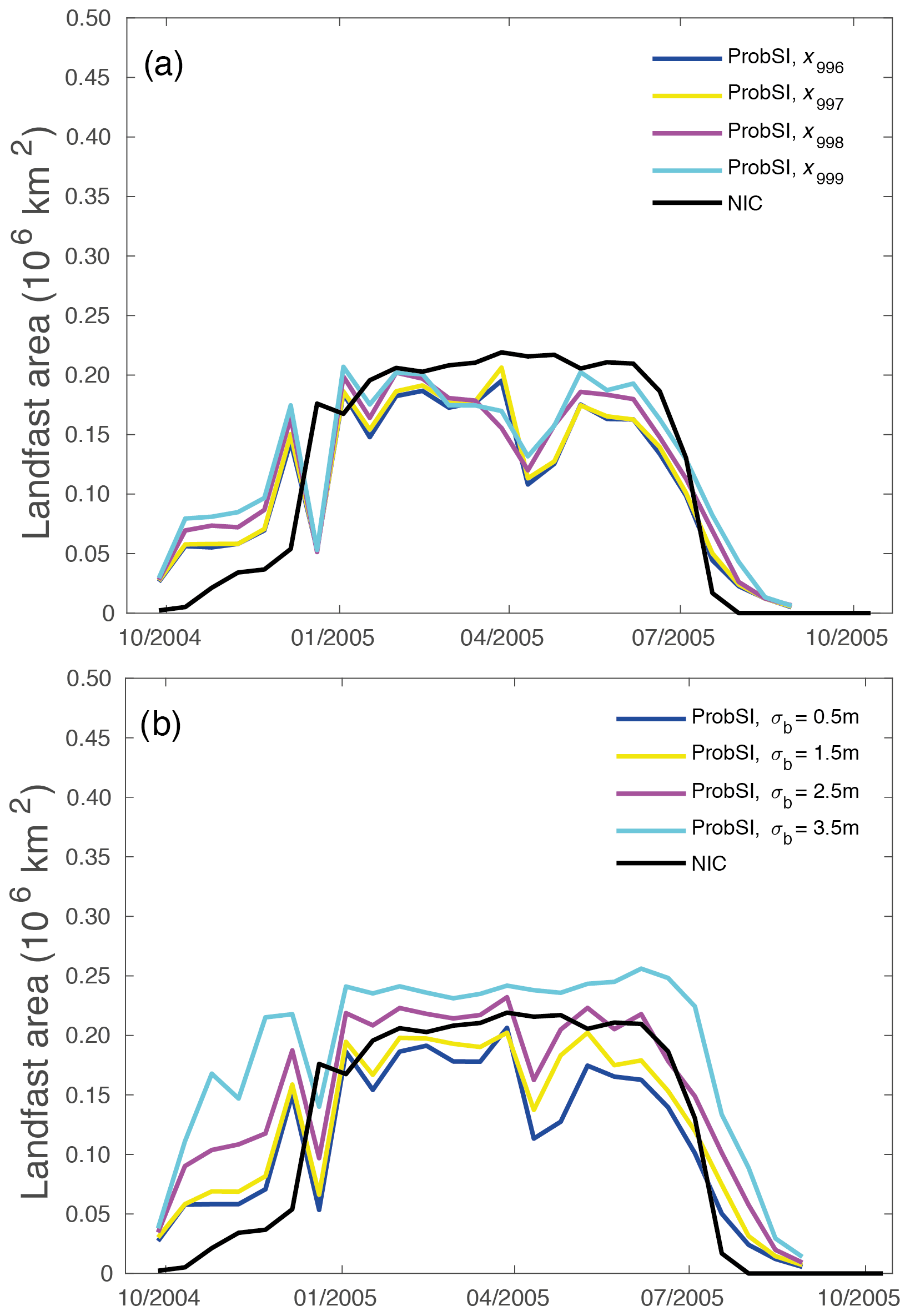
Figure 6 Area of landfast ice in Laptev Sea during winter 2004–2005 simulated with the ProbSI formulation and compared to NIC data. Panel (a) shows results with σ_b=0.5 m and different values of x_p, while panel (b) shows results with x₉₉₇ and different values of σ_b.

In regions of recurrent landfast ice, as in the Laptev and East Siberian seas (Fig. 7), the seabed stress is compared for the same date. The ProbSI and LKD stresses are non-zero in mostly the same spots. The ProbSI stress displays more low values in the deeper parts (the scale is logarithmic in the figure), which is the result of LKD having a flatter plateau followed by a sharper cutoff with increasing water depth as illustrated previously in Fig. 3. Following the same reasoning but for decreasing water depth, the hotspot values are larger in ProbSI. However, more important is that their locations – the landfast anchoring points – are the same in both formulations, which ensures a similar representation of the landfast ice.

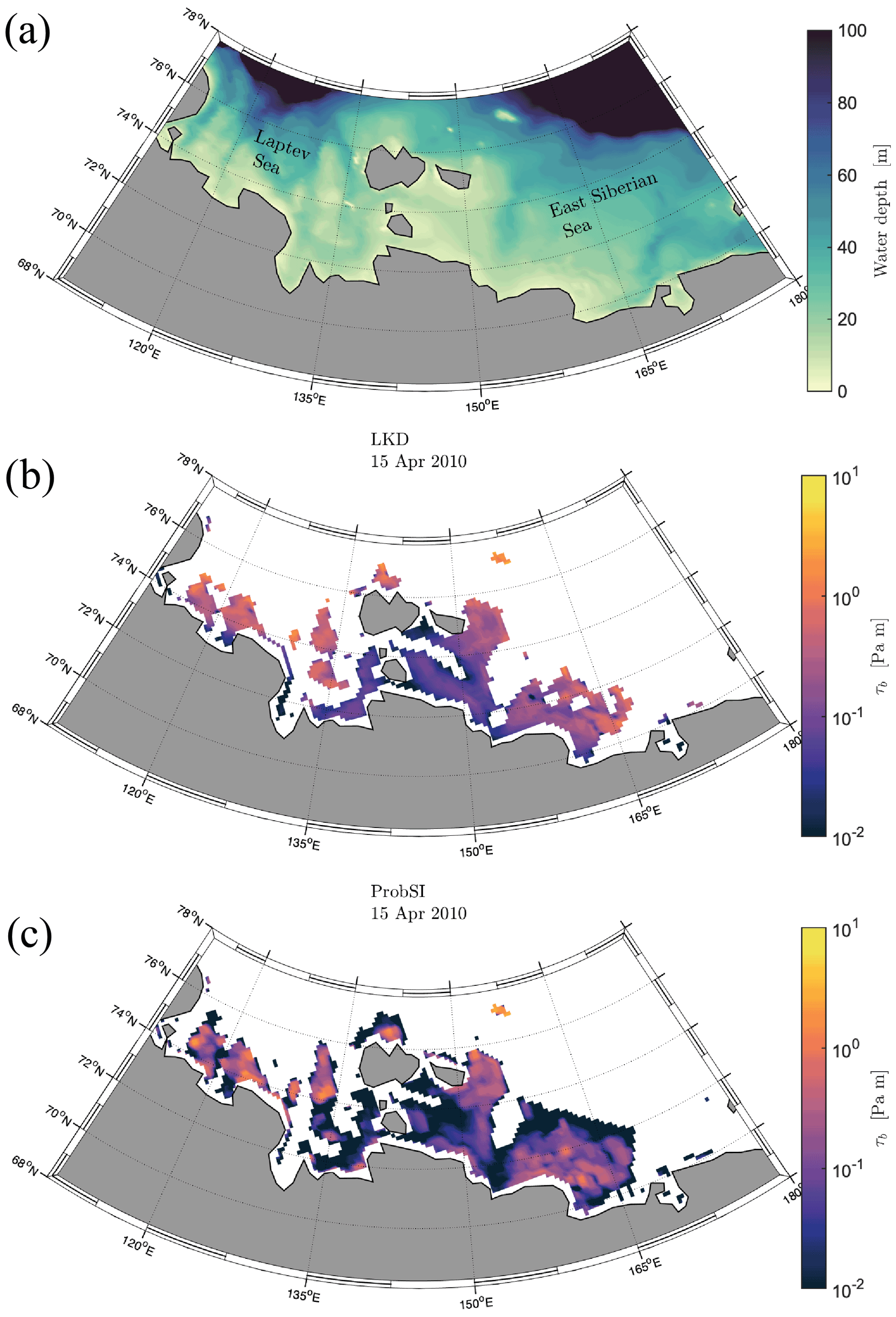
Figure 7 Water depth (a) and basal stress due to seabed–ice interaction in the Laptev and East Siberian seas on 15 April 2010 for the LKD (b) and ProbSI parameterizations (c).

The interannual variability in landfast area is then investigated over the different Siberian seas in Fig. 8. The simulated area in all seas is very similar using both methods and is in general very close to the one given by the proxy observations. The two methods are especially close in Kara Sea where we expect indeed less contribution from grounding to the landfast ice formation (L15; Lemieux et al., 2016). The East Siberian Sea exhibits some bi-modal distribution of the extent of the landfast ice (the larger mode is present in 2005, 2006 and 2010 while the smaller mode is visible in almost all years) that both methods capture. Only in Kara Sea, can both methods overestimate the area and in one year in particular by almost a factor of 2. Interestingly, ProbSI exhibits breakup events in the middle of the season in Laptev Sea that would require further investigation but otherwise is close to LKD and the proxy. ProbSI is again able to reproduce the LKD results, although we note that the onset of the landfast period is always earlier in ProbSI. This means that strong modelled ridging events happen quite early in the sea ice season. The ice chart information tends to show a slower onset, even relative to LKD. Later in the season and in the East Siberian and Laptev seas in particular, the opposite is visible; i.e. the landfast area is larger in LKD than in ProbSI. This indicates that, with overall thermodynamic growth, LKD responds with an associated deeper keel and larger regions of grounding whenever possible. In contrast, in ProbSI the deepest keel is more dominated by (early) local deformation, and therefore less inclined to increase during the season. The timings of the breakup of the landfast ice cover are similar for both parameterizations and agree reasonably well with the observations. However, the decrease in the simulated area of landfast ice is not as sharp as in the observations.

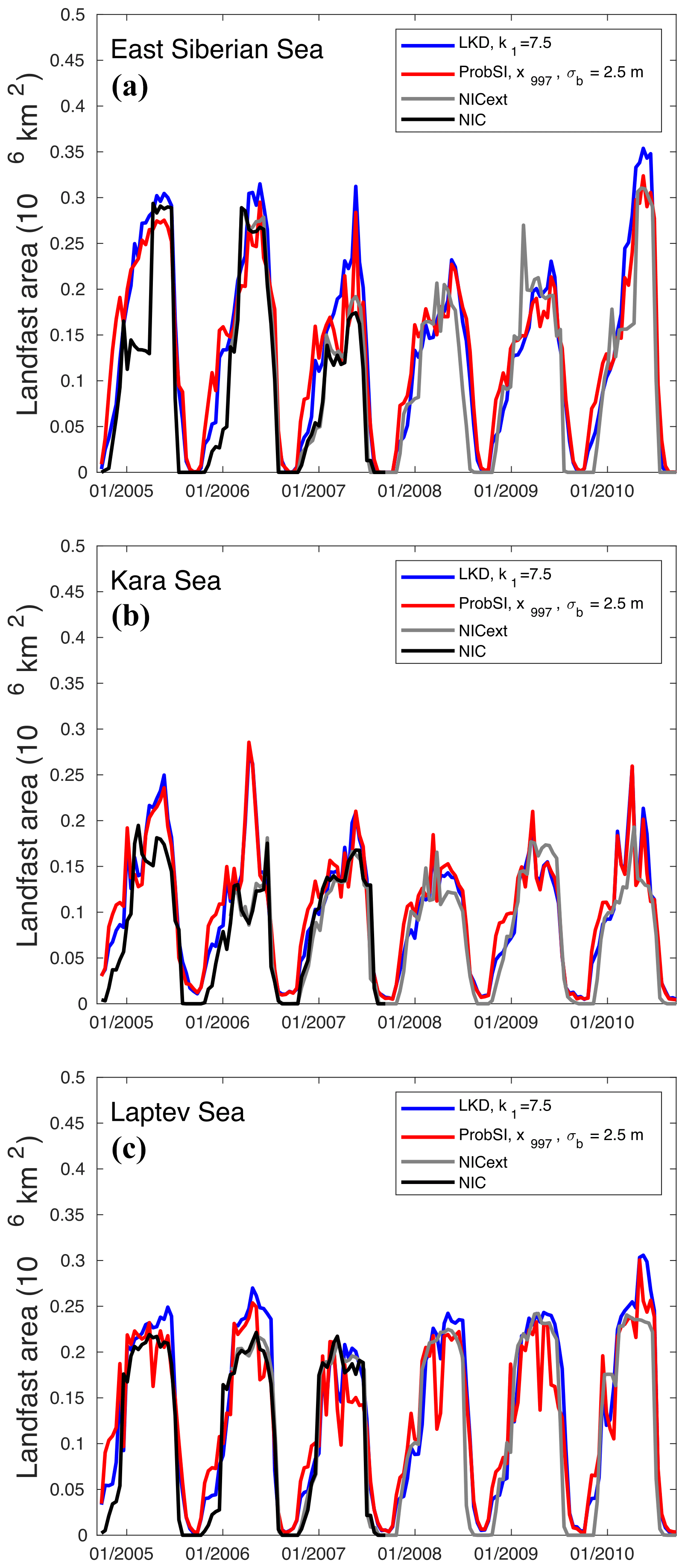
Figure 8 Area of landfast ice in the East Siberian Sea (a), the Kara Sea (b) and the Laptev Sea (c) as a function of time. The blue curves are for LKD while the red ones are for $x_{k_{max}}=x_{\mathrm{997}}$ and σ_b=2.5 m. In the three figures, the bold black curve is the area calculated from the NIC data while the grey curve is the extended database produced with the same method.

As introduced by Laliberté et al. (2018), we also computed the mean number of months of landfast ice per year over the 6-year period of the simulations (September 2004 to September 2010). Despite the earlier onset of the landfast regions in ProbSI, the overall period of landfast cover is similar to that of LKD over the Siberian shelves (Fig. 9). However, ProbSI displays a lower number of landfast months in the central Laptev Sea, where ProbSI is more prone to breakup events as seen already in the high-frequency fluctuations in Fig. 8c. Nonetheless, the difference in other parts of the Arctic Ocean is very small or not significant as in the CAA, where we expect landfast ice to be due mainly to the formation of ice arches (i.e. land-lock regions). We note though that both parameterizations overestimate landfast ice in some parts of the CAA because tides are not included in these simulations (Lemieux et al., 2018).

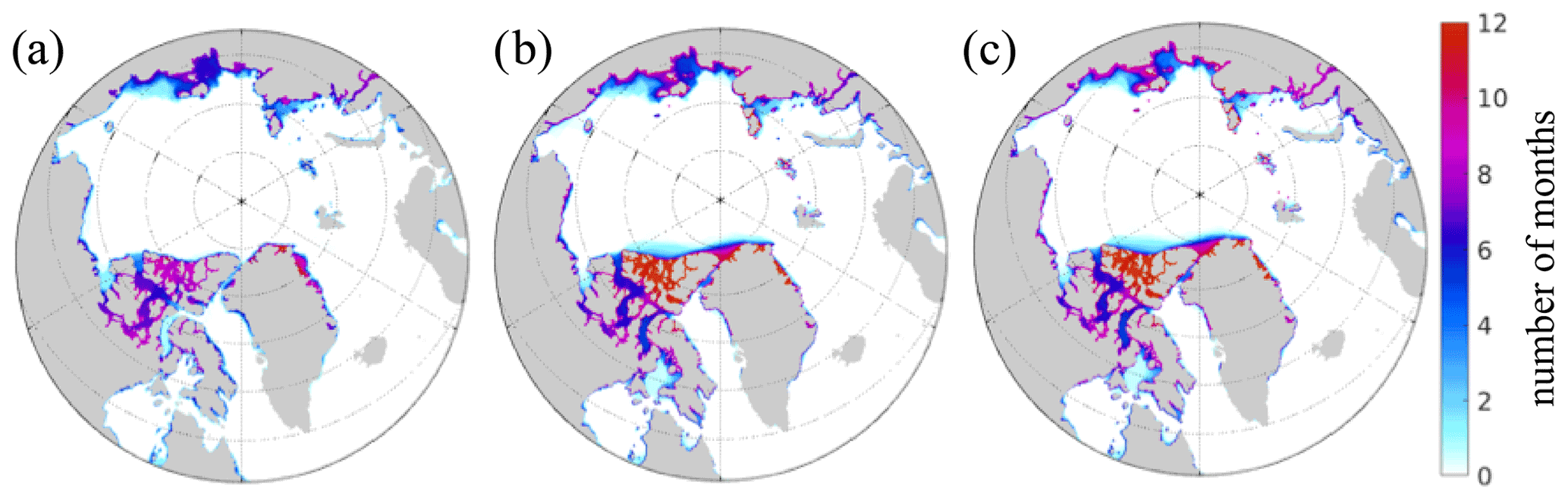
Figure 9 A 6-year average of the number of months per year during which the ice is landfast (a) obtained from the NIC charts and extensions, (b) with the LKD parameterization and (c) the ProbSI model with σ_b=2.5 m.

5 Discussion

A probabilistic approach to sea ice grounding based on the ITD information and PDFs of the bathymetry is proposed and compared to the simpler LKD approach. We illustrate the need for tuning one important parameter, mainly the percentile thickness at which the seabed stress calculation is truncated. Here, we selected the 99.7th percentile of the equivalent log-normal distribution, x₉₉₇, after a comparison with observations of the deepest keel to level ice thickness relations by Melling and Riedel (1996) and Amundrud et al. (2004) and a sensitivity analysis of the model compared with observed landfast ice cover in the Arctic.

The model simulations show a significant sensitivity to the standard deviation of the bathymetry distribution that we simply represent here as a truncated Gaussian having a value of 2.5 m over the entire domain after comparison with ice charts.

The coupled ice–ocean model is then run over the Arctic over a longer period to illustrate the difference between LKD and ProbSI methods over multiyear timescales. Results show that the onset of the landfast period happens more abruptly with the probabilistic approach. However in general the results are very close, i.e. within the 1-month error margin associated with the definition of the landfast ice cover. The stronger onset is likely due to early deformation events captured by the model. This is however not well supported by ice chart information. Selyuzhenok et al. (2015) suggest another explanation, namely that a stronger-than-observed resistance of the model to deformations can also contribute to the landfast ice formation. Another hypothesis that Selyuzhenok et al. (2017) put forward is that the thin and loose ice can still be mobile despite the presence of ridged features anchored to the bottom. In all cases, an in-depth analysis is required to investigate what is behind this discrepancy. By refitting the ITD to a log-normal distribution using the mean and variance, it is expected that the ProbSI method may be less reliable when the ice is thin. For example, forming new thin ice might in some cases lower the variance, thereby lowering the keel depth and reducing the friction with the seabed. This is maybe what explains break-up events in ProbSI that do not happen in LKD in the Laptev Sea (see in Fig. 8).

Nonetheless, because this method uses a somewhat more realistic representation of maximum keel depths, discrepancies between results and observations are prone to highlight problems or caveats in other aspects of the model, such as sea ice dynamics, ridging schemes, ITD resolution, or insufficient or bad bathymetry data in some areas. In particular, we stress the importance of retaining subgrid-scale bathymetry information in order to better constrain μ_b and σ_b.

Obtaining x₉₉₇ as an estimation of the deepest keel depth was done by looking at relatively thick and highly deformed ice. The discrepancies noted between LKD and ProbSI in marginal ice zones (e.g. Fig 5d) were not investigated, as it was not the focus of the paper and should be interpreted with care. Sea ice dynamics and thickness redistribution are potentially influenced by processes associated with surface ocean waves propagating into the ice cover such as fragmentation and rheology (Dumont et al., 2011; Boutin et al., 2020) that are under study by other authors. Nonetheless, the fact that x₉₉₇ is significantly different than x_k1 in Fram Strait, a region where highly deformed ice cohabits with new ice formed in leads and cracks, is consistent with the fact that the maximum keel depth is a nonlinear function of the mean ice thickness, which is duly taken into account by ProbSI.

The probabilistic approach to estimate the deepest keel depths from numerical sea ice models opens up a few interesting perspectives for research and applications. For instance, a probability of finding very thick sea ice, which constitutes a hazard for ice-going ships, can be easily diagnosed from the log-normal distribution. It also opens up the possibility to introduce icebergs directly within the model ITD, instead of modifying the model land–ocean mask, as is done by Van Achter et al. (2022), to take into account their role in the stability, location and timing of landfast ice covers. Finally, a closer inspection of landfast ice formation and rupture in the model in comparison with adequate observations is needed in order to further refine the method and understand the local and non-local impacts of seabed–ice interactions on other aspects of sea ice dynamics.