the Creative Commons Attribution 4.0 License.
the Creative Commons Attribution 4.0 License.
 | 17 Jan 2022
Sentinel-1 snow depth retrieval at sub-kilometer resolution over the European Alps
Hans Lievens
Isis Brangers
Hans-Peter Marshall
Tobias Jonas
Marc Olefs
Gabriëlle De Lannoy
Seasonal snow is an essential water resource in many mountain regions. However, the spatio-temporal variability in mountain snow depth or snow water equivalent (SWE) at regional to global scales is not well understood due to the lack of high-resolution satellite observations and robust retrieval algorithms. We investigate the ability of the Sentinel-1 mission to monitor snow depth at sub-kilometer (100 m, 500 m, and 1 km) resolutions over the European Alps for 2017–2019. The Sentinel-1 backscatter observations, especially in cross-polarization, show a high correlation with regional model simulations of snow depth over Austria and Switzerland. The observed changes in radar backscatter with the accumulation or ablation of snow are used in an empirical change detection algorithm to retrieve snow depth. The algorithm includes the detection of dry and wet snow conditions. Compared to in situ measurements at 743 sites in the European Alps, dry snow depth retrievals at 500 m and 1 km resolution have a spatio-temporal correlation of 0.89. The mean absolute error equals 20 %–30 % of the measured values for snow depths between 1.5 and 3 m. The performance slightly degrades for retrievals at the finer 100 m spatial resolution as well as for retrievals of shallower and deeper snow. The results demonstrate the ability of Sentinel-1 to provide snow estimates in mountainous regions where satellite-based estimates of snow mass are currently lacking. The retrievals can improve our knowledge of seasonal snow mass in areas with complex topography and benefit a number of applications, such as water resource management, flood forecasting, and numerical weather prediction. However, future research is recommended to further investigate the physical basis of the sensitivity of Sentinel-1 backscatter observations to snow accumulation.
- Article
(19987 KB) - Full-text XML
- BibTeX
- EndNote


In the European Alps, the release of precipitated water to discharge is delayed by storage in snow and glaciers. During the spring and summer, when water demand is high, snow and glacier meltwater sustains the more than 14 million inhabitants across 8 countries within the Alpine region, e.g., by supplying water for domestic use, industry, hydropower production, agriculture, etc. However, climate change causes mass loss of most glaciers (Zemp et al., 2019) and perturbs snowmelt dynamics (Bormann et al., 2018; Pulliainen et al., 2020), changing the timing and magnitude of water availability (Immerzeel et al., 2020). An improved monitoring of snow water resources can help strengthen our understanding of these changing hydrological processes in mountain regions.
Remote sensing can play an essential role in the monitoring of snow water resources. The current operational satellite retrievals of snow depth (or snow water equivalent, SWE, using auxiliary snow density information) rely primarily on passive microwave observations, either based only on remote sensing data (Kelly et al., 2003) or in combination with in situ measurements as in GLOBSNOW (Takala et al., 2011). Unfortunately, passive microwave observations have shortcomings, especially in mountain areas. The coarse footprints (∼25 km) cannot resolve the high spatial variability in snow depth imposed by complex topography (Dozier et al., 2016), and the microwave observations have a tendency to saturate at ∼0.8 m snow depth, which is often exceeded in mountains (Foster et al., 2005; Tedesco and Narvekar, 2010). Furthermore, missing details about the snow microstructure and layering complicate the physically based retrievals (Lemmetyinen et al., 2018). Therefore, new and robust satellite observations are critically needed to fill the mountain snow observation gap (Bormann et al., 2018).
Active microwave observations from synthetic aperture radar (SAR) show promise for mapping snow depth or SWE at a high spatial resolution. The optimal frequencies for global-scale snow observations are likely within X- to Ku-band (∼8–18 GHz) (Rott et al., 2010), based on their strong scattering within the snow volume (Yueh et al., 2009; King et al., 2015). Unfortunately, high-resolution Ku-band satellite observations are not available at present. Alternatively, the use of SAR interferometry (InSAR) (Guneriussen et al., 2001; Leinss et al., 2015; Conde et al., 2019) allows for the tracking of changes in SWE from changes in the radar signal phase that are caused by refractions in the snowpack. For this approach, lower frequencies such as L-band (1–2 GHz) are preferred, maintaining a better coherence between repeat observations. A number of future missions are addressing the use of L-band InSAR for snow applications, such as the National Aeronautics and Space Administration (NASA)–Indian Space Research Organisation (ISRO) SAR (NISAR) and potentially the Radar Observing System for Europe – L-Band (Rose-L).
Currently, routine SAR backscatter observations with a high spatial resolution (∼20 m) and frequent revisit (< weekly) are only available at C-band (5.4 GHz) from the European Space Agency (ESA) and Copernicus Sentinel-1 (S1) mission. Despite the availability of these routine observations, limited attention has been paid to the use of C-band backscatter for snow monitoring after earlier satellite observations had shown a limited sensitivity (Rott and Nagler, 1993; Bernier and Fortin, 1998; Bernier et al., 1999; Shi and Dozier, 2000). However, these studies were mostly focused on relatively shallow snow depths (below ∼1 m) and were investigating the use of backscatter observations in co-polarization. At C-band, co-polarized backscatter is generally dominated by (i) the scattering from the ground surface (depending on the moisture content and the temperature or freeze–thaw state of the soil) in dry snow conditions or by (ii) the absorption by liquid water in wet snow conditions (Baghdadi et al., 1997; Nagler and Roth, 2000; Luojus et al., 2007; Nagler et al., 2016).
Although further research is needed to improve our basic understanding of the physical scattering mechanisms, we hypothesize that cross-polarized observations at C-band are more sensitive to dry snow accumulation than co-polarized observations for two main reasons. First, the surface scattering from the ground is significantly weaker in cross-polarization due to the limited depolarization that occurs at the ground surface, especially for smooth surfaces. Second, dry snow is expected to enhance scattering in cross-polarization. More specifically, dry snow represents a multi-layered, dense medium of irregularly shaped (anisotropic) ice crystals that can form larger-scale clusters. Enhanced signal depolarization can for instance occur due to scattering within the dense anisotropic snow volume, multiple scattering on snow layer interfaces, and snow–ground scattering interactions (Du et al., 2010; Chang et al., 2014; Leinss et al., 2016). Hence, in cross-polarized observations, the scattering from the ground surface may no longer dominate over the scattering from the snow (Shi and Dozier, 2000; Pivot, 2012), especially for deep snow that is often encountered in mountain regions.
Recently, Lievens et al. (2019) demonstrated the sensitivity of S1 cross-polarized backscatter observations to dry snow accumulation and developed an empirical change detection algorithm to retrieve snow depth at 1 km spatial resolution over all mountain ranges in the Northern Hemisphere. The retrievals are based on a number of assumptions that, in the case of C-band, are likely more valid for deeper snow. That is, (i) an increase in snow depth causes an increase in snow scattering especially in cross-polarization; (ii) the snow scattering contribution is not negligible compared to the ground scattering contribution; and (iii) the ground scattering contribution remains relatively constant during the winter period because of the limited changes in soil temperature (due to the insulating properties of snow), soil moisture, and surface roughness, such that (iv) the main changes in backscatter over time can be related to changes in the snowpack.
Here, we further refine the S1 snow depth retrievals and evaluate them at 100 m, 500 m, and 1 km resolutions over the European Alps for August through April 2017–2018 and 2018–2019. First, the sensitivity of the S1 backscatter observations in co- and cross-polarization is evaluated using regional model simulations of snow depth over Austria and Switzerland. Thereafter, the S1 snow depth retrievals are compared against the model simulations, stratified by elevation and forest cover fraction. Finally, the accuracy of the retrievals is estimated based on independent time series measurements at 743 in situ locations across the Alps.
The results of this study contribute to improving our knowledge of seasonal snow mass in areas with complex topography and thereby address a long-standing observation gap in remote sensing of the cryosphere. A strong asset is the assured long-term continuity of S1 C-band SAR observations over the coming decades, which will allow for the analysis of trends in snow mass impacted by climate variability or climate change. Finally, the S1 snow depth retrievals could be of high value for data assimilation into land surface models (Girotto et al., 2020). Not only could the assimilation ensure improved and continuous (in time and space) estimates of various snow variables, it is likely to also benefit applications such as flood forecasting (Dechant and Moradkhani, 2011; Griessinger et al., 2019) or numerical weather prediction (de Rosnay et al., 2014). Future research is recommended to further investigate the physical scattering mechanisms in snow at C-band, including the impacts of snow microstructure and stratigraphy, and to extend the validation over regions with different soil, vegetation, and snow conditions, also using validation data at the matching scale of the satellite retrievals.
2.1 Sentinel-1 observations
The S1 mission is a constellation of two satellites, S1A and S1B, launched in April 2014 and 2016, respectively. Each of the satellites has an exact 12 d repeat cycle, completing 175 orbits per cycle. As both satellites share the same orbital plane with a 6 d offset, the two-satellite constellation offers an exact 6 d repeat cycle. Depending on the region, more frequent observations (every 2–3 d on average) are available due to orbits with partly overlapping swaths and the combination of ascending and descending tracks. Note that over repeating cycles, acquisitions from a given orbit consistently observe the same grid cell with the same incidence and azimuth angle and should thus provide repeated samples that are not impacted by the satellite viewing geometry. However, observations from different orbits can be biased relative to each other due to the different viewing geometries.
Over land and outside the polar regions, S1 routinely operates in the Interferometric Wide Swath (IW) mode, acquiring backscatter observations at ∼20 m resolution in vertical–vertical (VV) and vertical–horizontal (VH) polarizations. We processed the IW S1A and S1B ground-range-detected (GRD) data over the European Alps for 2017 to 2019 (∼4600 images). The processing was performed using the ESA Sentinel Application Platform (SNAP) toolbox, applying standard processing techniques: precise orbit file application, GRD border noise removal, thermal noise removal, radiometric calibration, terrain flattening to backscatter as γ0 (Small, 2011; Small et al., 2022), range-Doppler terrain correction, aggregation to 100 m by averaging in linear scale, and projection onto the World Geodetic System WGS84 geographic coordinate system. The terrain flattening and terrain correction were applied using digital elevation data from the Shuttle Radar Topography Mission (SRTM) at 1 arcsec resolution, which is similar to the original resolution of S1. Observations with a local incidence angle were excluded to reduce radar shadowing effects. The 100 m grid cell size in the processed output was chosen to reduce the speckle noise inherent to radar observations, to reduce the impacts of geometric distortions within the complex topography of the Alps (e.g., radar foreshortening, layover, shadowing, and inaccuracies in the geo-referencing), and to enhance the feasibility of the processing by reducing the processing time and storage requirements.
2.2 Snow depth retrievals
The snow depth retrieval algorithm is based on the assumption that part of the microwave signal depolarizes in the snowpack, for instance by the scattering on anisotropic clusters of snow crystals within the snow volume (Chang et al., 2014), by the multiple scattering between snow layer interfaces (Du et al., 2010), or by snow–ground scattering interactions. A deeper snowpack is likely to result in more opportunities for signal depolarization and in stronger scattering in cross-polarization. Hence, the strength of the cross-polarized scattering can be related to snow depth. While higher microwave frequencies (such as X- and Ku-band) are likely more suitable to detect snow scattering in shallow snow environments, we hypothesize that the contribution at C-band is large enough for application to the typically deep snow regimes in mountain areas. The algorithm further assumes that snow scattering generally has a stronger contribution in cross-polarized (VH in the case of S1) compared to co-polarized (VV) observations, whereas scattering impacts from soil moisture, soil freeze or thaw, or soil temperature are expected to be more similar in co- and cross-polarization. Therefore, the use of a ratio (in linear scale or difference in dB scale) between cross- and co-polarization γ0 observations can reduce the impacts of ground, vegetation, and surface geometry properties and enhance the sensitivity to snow depth (Lievens et al., 2019). As auxiliary input, the algorithm requires snow cover (SC) absence or presence observations, which we derived from the 1 km resolution Interactive Multisensor Snow and Ice Mapping System (IMS; National Ice Center, 2008); glacier cover derived from the Randolph Glacier Inventory 6.0 (RGI Consortium, 2017); and forest cover fraction (FCF) derived from the 100 m Copernicus PROBA-V dataset (Buchhorn et al., 2020).
The empirical retrieval method based on change detection builds further on Lievens et al. (2019), and the main differences with this study are highlighted in this section. Firstly, the algorithm has been modified to account for the observation that, for sparsely vegetated areas, a ratio of VH- and VV-polarized γ0 (cross-polarization ratio; CR) shows a higher temporal correlation with snow depth, whereas in forested areas, the VV-polarized γ0 shows a higher temporal correlation (see Fig. 6 below). The latter may be caused by the relatively stronger scattering contribution from forests (and vegetation in general) in VH polarization (Vreugdenhil et al., 2020), decreasing the sensitivity to the underlying snowpack. Therefore, two backscatter changes ( and ; dB) are calculated for each location i between the observations at time t and tpri (either 6, 12, 18, or 24 d ago) from the same relative orbit:
where represents a weighted combination of cross-polarized and co-polarized observations (dB) of the general form
with A being a fitting parameter. Further, and are scaled and combined based on the PROBA-V forest cover fraction (FCF (–); ranging from 0 to 1):
with B an empirical parameter to scale the CR and VV contributions. Δγ0 is clipped to ±3 dB to prevent γ0 outliers from propagating into the retrieval. In glaciated areas, Δγ0 is reduced by an empirical scaling coefficient, which linearly increases from 0.1 (strong reduction) on 1 August to 1 (no reduction) from January onwards. This reduces the impacts of typically strong increases in γ0 during early autumn, which we hypothesize are likely caused by the freezing of glacial meltwater. Future research is needed to investigate the validity and performance of the retrieval approach in glaciated areas.
The snow change detection index (SI; dB) at time t is then calculated by adding Δγ0 (dB) to the prior estimate of SI at tpri:
SI(i,t) is set to zero in case of negative values or when snow cover is absent. SI(i,tpri) is the weighted average SI over the previous repeat cycle (i.e., tpri±5 d):
with weights (wk) given by the inverse distance in time from tpri. This ensures that SI(i,t) also includes information obtained from different S1 orbits. Finally, SI (dB) is translated into snow depth (SD; in meters) by multiplication with an empirical scaling factor C:
The three algorithm parameters in Eqs. (3) to (7) were iterated over , , and and optimized based on model simulations of snow depth (optimization not shown; simulations described in Sect. 2.3). A and B were optimized by maximizing the spatio-temporal correlation between simulations and retrievals, whereas C was optimized by minimizing the bias. This resulted in A=2, B=0.5, and C=0.44, which are further used in this study over the entire time period and study domain. A caveat to the optimization based on model simulations is that simulation uncertainties can propagate into the retrieval.
Secondly, as an extension to Lievens et al. (2019), we here include a wet snow detection algorithm that allows the S1 retrievals to be flagged in wet snow conditions. Wet snow is known to absorb a large part of the radar signal, causing a strong decrease in backscatter (e.g., Baghdadi et al., 1997; Nagler and Roth, 2000; Luojus et al., 2007; Nagler et al., 2016; Marin et al., 2020). Therefore, the snow is classified as wet if (in locations where FCF < 0.5) or (in locations where FCF > 0.5) is lower than a certain threshold set to −2 dB. The snow also remains wet if the previous time step (tpri) was classified as wet, and γ0 did not increase by more than 2 dB (e.g., due to refreezing). Note that Δγ0 is calculated between consecutive observations from the same relative orbit. Therefore, a dry or wet snow retrieval from a given relative orbit does not impact the retrieval from another relative orbit. However, it is possible that dry and wet snow retrievals alternate between different relative orbits.
An additional wet snow detection criterion mainly addresses regions where no strong decrease in γ0 is observed due to a lower sensitivity to snow wetness. This is for instance expected in regions with shallow or patchy snow cover where the soil scattering contribution may dominate or in forested regions where the snow signal is attenuated, and the vegetation contributes to the scattering. There, the snow state is classified as wet if the SD retrieval becomes lower than zero while snow cover is present. If the snow was classified as wet for >50 % of the observations within the past two S1 repeat cycles (24 d), then the wet snow classification is retained until the snowpack has completely melted to avoid that uncertainties induced by wet snow accumulate into subsequent retrievals.
Note that we refrain from detecting wet snow based on the difference in γ0 with a constant dry snow reference value, as often done in the literature (e.g., Baghdadi et al., 1997; Nagler et al., 2016; Tsai et al., 2019; Manickam and Barros, 2020), because of the difficulty in accurately defining the dry snow reference value (Manickam and Barros, 2020). For instance, an average summer γ0 is often used as an approximation of the dry snow reference (Tsai et al., 2019; Manickam and Barros, 2020). However, in regions with dense vegetation, summer γ0 can be high due to vegetation contributions, causing an over-detection of wet snow in winter if γ0 is systematically lower. Conversely, in bare or sparsely vegetated regions, snow accumulation can cause a significantly higher γ0 (by several decibels) compared to the summer reference, requiring a large decrease from wet snow to reach the threshold below the summer reference (see below; e.g., Fig. 3). The use of a fixed dry snow reference value is here avoided by thresholding the decrease rate of γ0 over time instead.
Using the empirical framework outlined above, we processed snow depth retrievals for August through April 2017–2018 and 2018–2019 over the entire European Alps. The retrievals are performed at 100 m spatial resolution, but outputs are produced at three different spatial resolutions, i.e., 100 m, 500 m, and 1 km, to assess the impact of the spatial resolution on the retrieval performance. The 500 m and 1 km snow depth retrievals are obtained by linearly averaging the 100 m retrievals, with a reduced weight () assigned to wet snow pixels. The coarser-scale retrievals are omitted if only less than 30 % of the enclosed 100 m grid cells contain data and are classified as wet if less than 30 % remain after excluding the wet snow pixels.
2.3 Model simulations
Output from two regional snow models for Austria (SNOWGRID-CL) and Switzerland (OSHD) is used to assess the S1 backscatter and to optimize the snow depth retrievals. Figure 1 shows that the joint simulation domain covers a large part of the Alps. In addition, simulations by the Noah-Multiparameterization (Noah-MP) land surface model (Niu et al., 2011) are used to assess the impacts of soil moisture and soil temperature on S1 backscatter.
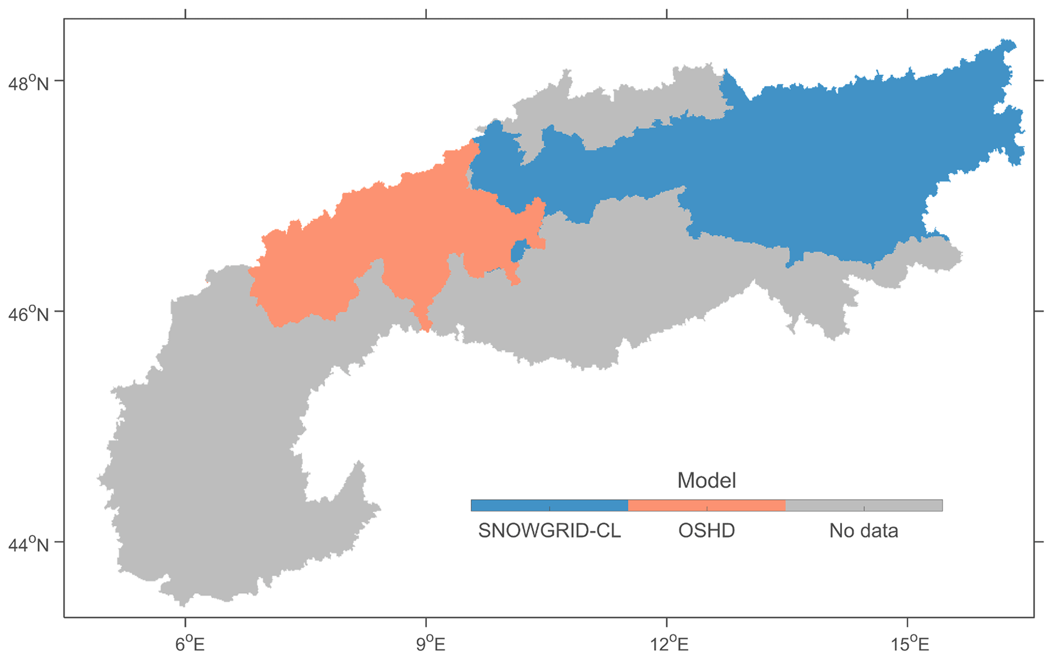
Figure 1The domains of the 1 km resolution SNOWGRID-CL and OSHD model simulations of snow depth.
SNOWGRID-CL (Olefs et al., 2020) is the climate version of the spatially distributed snow model run operationally at the ZAMG (Zentralanstalt für Meteorologie und Geodynamik) with a daily time step on a 1 km grid over Austria. The model outputs snow depth and SWE and is forced with daily 1 km gridded meteorological data of air temperature, precipitation, and evaporation that take into account the high variability in these variables in complex terrain (Hiebl and Frei, 2016, 2018; Haslinger and Bartsch, 2016). The model solves the shortwave radiation balance following Pellicciotti et al. (2005) and uses a simple two-layer snow scheme, considering settling, the exchange of heat and liquid water content, and energy addition by rain. Lateral snow mass redistribution is included as a function of snow and terrain properties (Frey and Holzmann, 2015). The accuracy of the daily snow depth simulations (correlation of 0.83, root mean square error (RMSE) of 14.11 cm, and bias of −3.12 cm) has been assessed for the period from November through April 2011–2018 (Olefs et al., 2020).
The OSHD (operational snow-hydrological service) multi-model framework provides daily SWE and snowmelt estimates for Switzerland at 1 km spatial resolution. It consists of a suite of spatially distributed snow models integrated with three-dimensional sequential assimilation of snow monitoring data from several hundred sites (Magnusson et al., 2014; Winstral et al., 2019). The models include procedures to account for unresolved variability at the sub-grid scale, two of which are (1) parameterizing fractional snow-covered area using terrain parameters derived at 25 m spatial resolution according to Helbig et al. (2015) and (2) considering snow distribution and redistribution at small scales using slope- and aspect-dependent transfer functions that were derived from a set of high-resolution snow depth maps from airborne lidar (Grünewald and Lehning, 2015). For this study we use output from the JULES Investigation Model (JIM; Essery et al., 2013), which is one of the OSHD members. JIM is forced using a combination of numerical weather prediction output from COSMO-1 (http://www.cosmo-model.org, last access: 30 April 2019) and reanalysis data as detailed in Winstral et al. (2019) and includes data assimilation from 344 Swiss snow monitoring stations. The assimilation improves the accuracy of the daily snow depth simulations from an RMSE of 21.3–42.4 cm and bias of 4.08–26.1 cm (varies between the years 2014, 2015, and 2017) to an RMSE of 17.3–25.6 cm and bias of 0.8–2.5 cm.
Additional simulations with the Noah-MP land surface model are performed to provide information on soil conditions (SNOWGRID-CL and OSHD are strictly snowpack models). These simulations cover the regional model domain at the 1 km spatial and daily temporal resolution and are forced using the globally available Modern-Era Retrospective Analysis for Research and Applications, Version 2 dataset (Gelaro et al., 2017). The analyzed model outputs include soil moisture (in m3 m−3) for the top soil layer (0–0.1 m) and soil temperature (in kelvin) for four soil layers (0–0.1, 0.1–04, 0.4–1, and 1–2 m).
2.4 In situ measurements
Daily in situ measurements of snow depth for the period of the satellite retrievals were collected from 743 sites, managed by Météo-France, the WSL – Institute for Snow and Avalanche Research SLF, and the ZAMG. The locations of the sites are shown in Fig. 2 on top of SRTM elevation and PROBA-V land cover. The minimum, mean, and maximum elevations of the measurement sites are 230, 1395, and 3114 m, respectively. The in situ time series are used to evaluate the temporal and spatial variability in the S1 retrievals in terms of Pearson correlation (R) as well as the bias and mean absolute error (MAE).

Figure 2The in situ measurement locations within the European Alps on top of (a) elevation (m) and (b) land cover class (–). ENF stands for evergreen needleleaf forest, DBF for deciduous broadleaf forest.
An inevitable problem in the comparison between S1 observations and in situ measurements is that, particularly in mountain areas, the point-scale snow conditions at the in situ sites do not always resemble the grid-scale conditions represented by the satellite data. The local variability in conditions can be large due to differences in elevation, slope, and aspect as well as wind and vegetation impacts on snow distribution (Blöschl, 1999; Seidel et al., 2016; Schattan et al., 2017). Moreover, in situ sites are preferentially located in relatively flat and non-forested terrain, often not representative of the surrounding area displaying large variations in slope and forest cover (Meromy et al., 2013; Grünewald and Lehning, 2015; Dozier et al., 2016), and sites are underrepresented at high elevations (see Fig. 2).
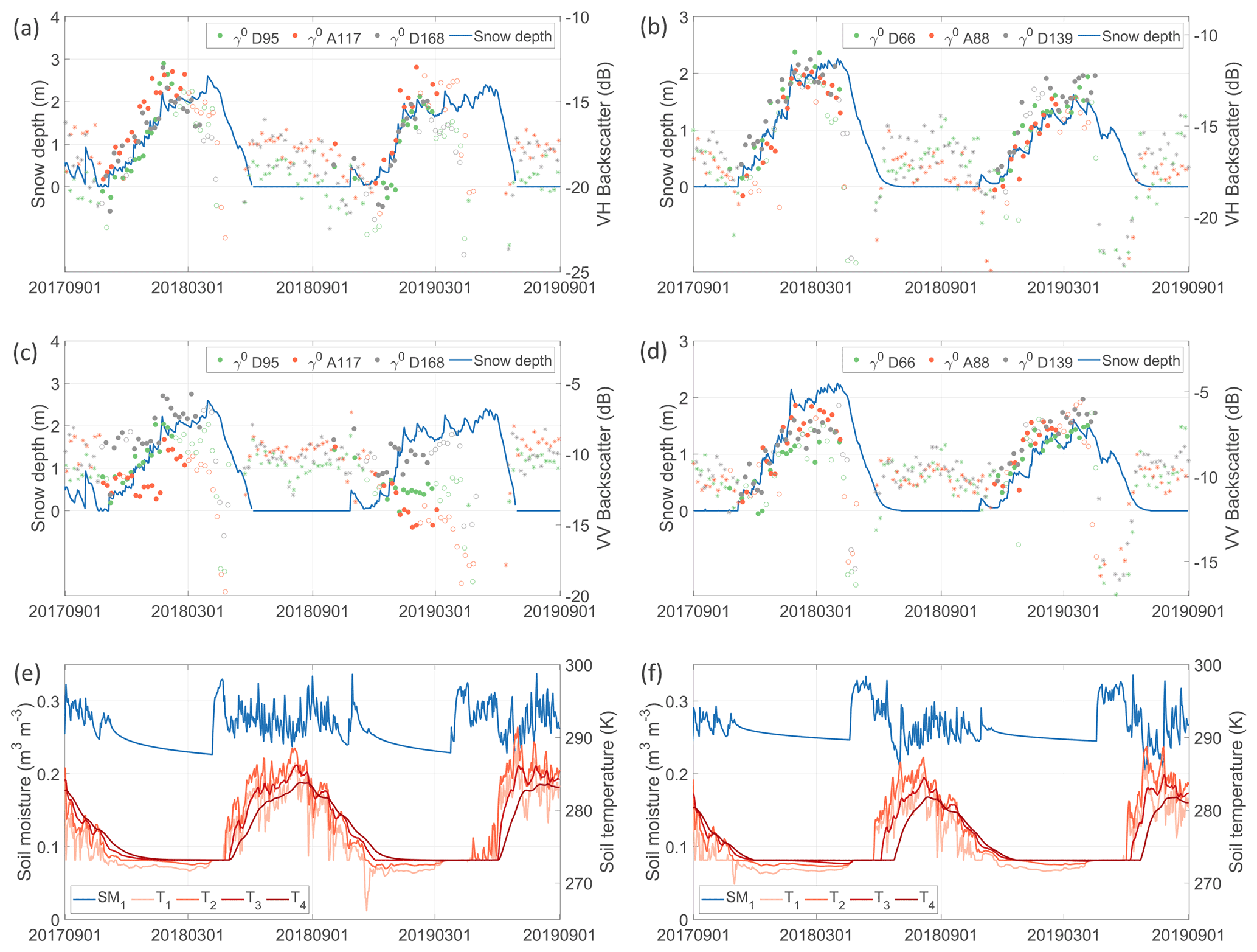
Figure 3Time series of S1 γ0 (dB) for three different orbits, in (a, b) VH polarization and (c, d) VV polarization, compared against model simulations of snow depth (m) for a grid cell in (a, c) Austria and (b, d) Switzerland. The γ0 observations during snow-free conditions (based on IMS SC) are displayed by * and those during wet snow conditions (based on S1) by open circles. The γ0 axes are scaled to enhance visualization. Panels (e) and (f) show corresponding model simulations of soil moisture (SM1: 0–0.1 m; in m3 m−3) and soil temperature (T1: 0–0.1 m; T2: 0.1–04 m; T3: 0.4–1 m; and T4: 1–2 m; in kelvin) from the Noah-MP land surface model.
3.1 Comparison of S1 observations with snow model simulations
3.1.1 S1 backscatter
Figure 3 shows time series examples for two locations, one in Austria (47.1379∘ N, 11.5923∘ E; 2355 m) and one in Switzerland (46.0962∘ N, 7.2569∘ E; 2140 m). The time series compare 100 m γ0 observations in VH and VV polarization with the nearest 1 km model simulations of snow depth from SNOWGRID-CL (Austria) and OSHD (Switzerland) and soil moisture and soil temperature from Noah-MP. The γ0 observations in Austria are shown separately for three selected orbits, i.e., descending orbit 95 (D95), ascending orbit 117 (A117), and D168, corresponding with local incidence angles of 26.5∘, 61.9∘, and 17.8∘, respectively. The γ0 observations in Switzerland are shown for D66 (55.8∘), A88 (32.9∘), and D139 (46.9∘).

Figure 4(a) The simulated yearly maximum snow depth (m) at 1 km resolution from August through April, averaged over 2 years (2017–2018 and 2018–2019). (b) The PROBA-V forest cover fraction (–) and Randolph Glacier Inventory (RGI) glacier cover.
The observations (Fig. 3a and b) show a consistent and strong correspondence with dry snow accumulation at both locations and for both winter seasons. Limited differences are observed between the orbits, which can be explained by the different local incidence angles (also impacting the travel path lengths through the snow), azimuth angles, and overpass times (06:00 LT for D, 18:00 LT for A). The evolution in is unlikely to be related to changes in soil moisture or soil temperature (Fig. 3e and f). Soil moisture shows a decrease throughout the snow accumulation period, and this would result, if it would have any impact, in a decrease in γ0. Soil temperature remains nearly constant throughout the snow accumulation period due to the insulating properties of snow. Near the peak of the snow season, the strong decrease in γ0 is caused by the increase in liquid water content within the snowpack that absorbs the radar signal. The wet snow detection algorithm effectively tracks the onset of the wet snow conditions and allows for the masking of subsequent observations (shown by open circles). Note that the first wetting of the snow typically starts before the actual melting phase with shrinking of the snowpack (Marin et al., 2020). The observations (Fig. 3c and d) correspond reasonably well with the snow depth simulations for the location in Switzerland but less for the location in Austria, in particular during the winter of 2018–2019. There, the is likely impacted more strongly by the conditions of the ground surface, while also larger differences in backscatter are observed between orbits.
Further, the impact of snow accumulation on S1 backscatter is investigated over the spatial domain covered by the regional models. Figure 4 shows the maximum snow depth (m) between August and April (yearly maximums, averaged over 2017–2018 and 2018–2019) based on the 1 km model simulations from SNOWGRID-CL and OSHD, along with 100 m fractional forest cover from PROBA-V. Correspondingly, Fig. 5 shows the 100 m S1 backscatter changes (Δγ0) between the days with simulated maximum snow depth and first snow cover, excluding wet snow conditions detected by S1. Note that the day with maximum simulated snow depth varies by location. Δγ0 is first calculated per relative orbit and subsequently averaged across the different orbits.
In regions with shallow maximum snow depths (<1 m), generally remains relatively constant, with changes typically within ±2 dB (Fig. 5a). Most of the regions with significant snow accumulation, outside glaciated areas, show a slight increase in (about 1–3 dB). The underlying physical mechanisms that cause this increase are still uncertain, but we hypothesize that, in addition to snow volume scattering, the frequent occurrence of snowmelt–refreeze cycles may lead to a more complex snowpack with pronounced layering (including ice crusts and frozen percolation features) that increases scattering in co-polarization. The increase is mainly observed in areas with a lower during snow-free conditions (not shown). In other regions, particularly at high elevations (above ∼2400 m, but not in glaciated areas), a slight decrease in is observed. At these elevations, melt–refreeze cycles are much less frequent, causing a more homogeneous snowpack, from which the scattering contributions in co-polarization are lower compared to the contributions from the ground surface. The slight decrease in in these regions is likely caused by the attenuation of the ground surface scattering by the snowpack. Finally, in glaciated areas, a moderate to strong increase (4–5 dB or more) is observed, which is likely due to the gradual freezing of glacial meltwater during winter, reducing the absorption of the radar signal through winter.

Figure 5Changes in 100 m S1 backscatter (γ0; dB) with snow accumulation: the γ0 of the day with the maximum simulated snow depth (between August and April) minus the γ0 of the first day with snow cover, for (a) VV polarization, (b) VH polarization, and (c) the cross-polarization ratio (CR). Wet snow conditions detected by S1 are excluded.
These results are in close agreement with several previous studies. Rott and Nagler (1993) found a slight decrease in European Remote Sensing (ERS) VV-polarized backscatter observations over a shallow snowpack but a strong increase over glaciated areas. Bernier and Fortin (1998) and Arslan et al. (2006) observed mostly an increase in co-polarized backscatter during dry snow accumulation, based on RADARSAT and airborne observations, respectively. Shi and Dozier (2000) and Pivot (2012) observed an increase in RADARSAT and ERS co-polarized backscatter (up to several decibels) with dry snow accumulation in regions where snow volume scattering was dominating over ground surface scattering and a slight decrease in regions where the dominant effect was the attenuation of the ground surface scattering by the snowpack.
The signature in (Fig. 5b) shows a more pronounced spatial pattern compared to , with a consistent and moderate to strong increase in (about 2–4 dB) in regions where snow depth reaches above 1 m. We hypothesize that for cross-polarized observations the scattering from the snowpack is more consistently dominating over the (attenuated) ground surface scattering. The ground scattering contribution is relatively lower since it is mostly in the form of surface scattering with limited depolarization (especially for smooth and sparsely vegetated surfaces). The dry snow scattering contribution is stronger, most likely because depolarization occurs after volume scattering on anisotropic crystals or clusters of crystals, multiple scattering on snow layer interfaces, and snow–ground scattering interactions. As in the observations, the largest increases in (>5 dB) are again observed over glaciated areas and are likely caused by the combination of freezing glacial meltwater and snow accumulation.
Only a few previous studies have investigated satellite or airborne cross-polarized backscatter observations at C-band in relation with snow depth or snow mass. Some of the heritage satellite missions, such as ERS, did not have the capability to measure in cross-polarization. Moreover, since the 90s, there has been a focus shift towards the use of higher-frequency microwave observations (e.g., in X- and Ku-band), in part due to the limited potential of C-band found with co-polarization, but also in preparation for higher-frequency satellite mission candidates (e.g., CoReH2O). Nevertheless, our results are in agreement with Arslan et al. (2006), who observed a stronger increase in cross-polarization than in co-polarization at C-band with dry snow accumulation. More recently, Lievens et al. (2019) demonstrated the sensitivity of S1 cross-polarized backscatter observations to snow depth over all Northern Hemisphere mountain ranges.
An exception to the overall stronger snow signal in S1 is observed in regions with both substantial snow accumulation and dense forest cover. Here, slightly larger differences are found for . We hypothesize this may be caused by the relatively stronger scattering from vegetation in cross-polarization (compared to co-polarization), reducing the sensitivity to the scattering contributions from the snowpack. At the same time, forested regions in the Alps are mostly present at lower elevations in the valleys (below ∼2500 m), where an increased occurrence of melt–freeze cycles could result in a more complex and layered snow structure that impacts the polarimetry. The (Fig. 5c) generally enhances the impact of snow, showing larger increases in backscatter for regions with deep snow compared to . The spatial distribution is however similar to that of , also showing slight decreases in in regions with shallow snow and forest cover, particularly in the western part of the model domain.

Figure 6The time series correlations between snow depth simulations (m) and 100 m S1 γ0 observations (dB) for August through April 2017–2018 and 2018–2019, for (a) VV polarization, (b) VH polarization, and (c) the cross-polarization ratio (CR). Zero snow depths (based on the model simulations) and wet snow conditions (detected by S1) are excluded.
Figure 6 illustrates the time series correlations between the 1 km model snow depth simulations (linearly interpolated to 100 m) and the corresponding 100 m S1 γ0 observations over the model domain for August through April 2017–2018 and 2018–2019. Note that the analysis excludes the time steps with zero snow depth (based on the model simulations) and time steps with wet snow (detected by S1). Consistent with the results shown in Figs. 3 and 5, the correlations for areas with a maximum snow depth above ∼1 m are considerably higher for (Fig. 6b) than for (Fig. 6a). The use of further enhances the time series correlation in areas at high elevation. However, results in higher correlations at lower elevations including forested regions. Therefore, these results support the use of different polarization combinations (i.e., CR and VV) for snow depth retrieval depending on the forest cover fraction (see Sect. 2.2).
3.1.2 S1 snow depth
Figure 7 shows the time series correlations between the 1 km model snow depth simulations (linearly interpolated to 100 m) and the corresponding 100 m S1 snow depth retrievals. These are generally higher than the corresponding correlations between snow depth and γ0 shown in Fig. 6. This mainly results from the re-initialization (i.e., SD = 0) at the start of every snow season, which removes differences in γ0 levels between years. Furthermore, Fig. 7a and b compare scenarios with and without the inclusion of zero snow depths. It shows that the inclusion of zero snow depths results in higher correlations mainly in regions with shallow and occasional snow (e.g., in eastern Austria). Nevertheless, it is important to remark that the S1 γ0 observations in these regions only show a weak (if any) correspondence with snow depth because of the weak scattering contributions from shallow snow, frequent wet snow and melt conditions, and the frequent disappearance and re-appearance of snow cover. The higher correlation values are therefore mainly attributed to the effectiveness of the IMS snow cover dataset, used as auxiliary input in the retrieval, to discern between the absence and presence of snow and should thus not be attributed to the S1 observations.
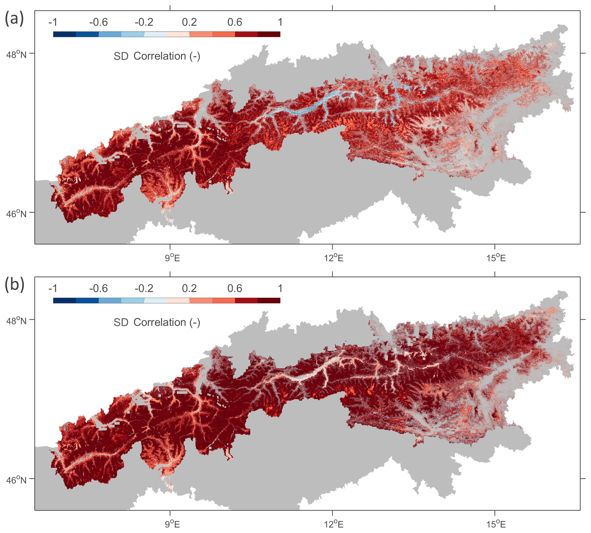
Figure 7The time series correlations between snow depth simulations (m) and 100 m S1 snow depth retrievals (m) for August through April 2017–2018 and 2018–2019, with (a) exclusion of zero snow depths (based on the model simulations) and (b) inclusion of zero snow depths. Wet snow conditions (detected by S1) are excluded in both cases.
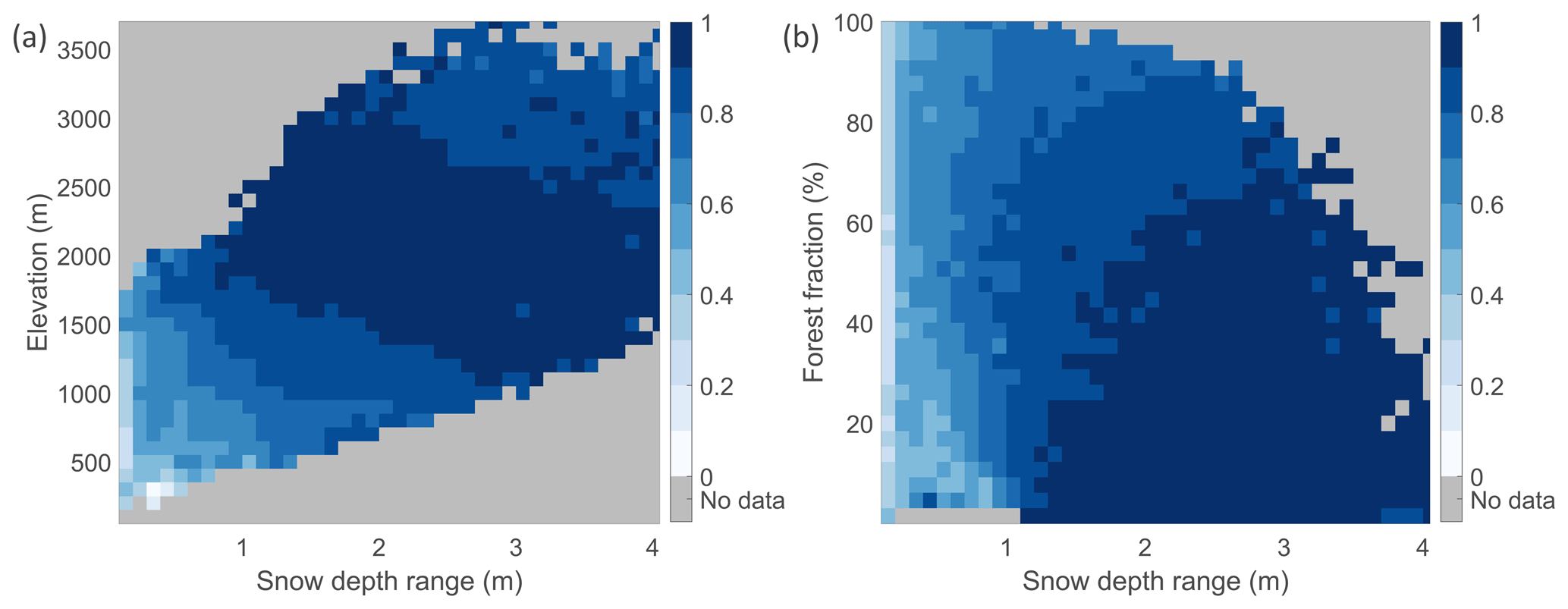
Figure 8The time series correlation between simulated and retrieved snow depth (m) at 1 km resolution, stratified by (a) elevation (m) and snow depth range (m) and (b) forest cover fraction (%) and snow depth range (m).
Figure 8 stratifies the time series correlations between the 1 km S1 snow depth retrievals and 1 km model snow depth simulations by the snow depth range (based on the model simulations) as well as elevation (from SRTM) and forest cover fraction (from the Copernicus PROBA-V dataset). The correlation generally exceeds 0.8 when the range in snow depth exceeds ∼1 m, except in areas with an elevation below ∼1000 m or a forest cover fraction above ∼80 %. The S1 retrievals are thus expected to be more accurate for the high snow regime (with snow depths reaching above 1 m) and in areas with lower forest cover fraction.
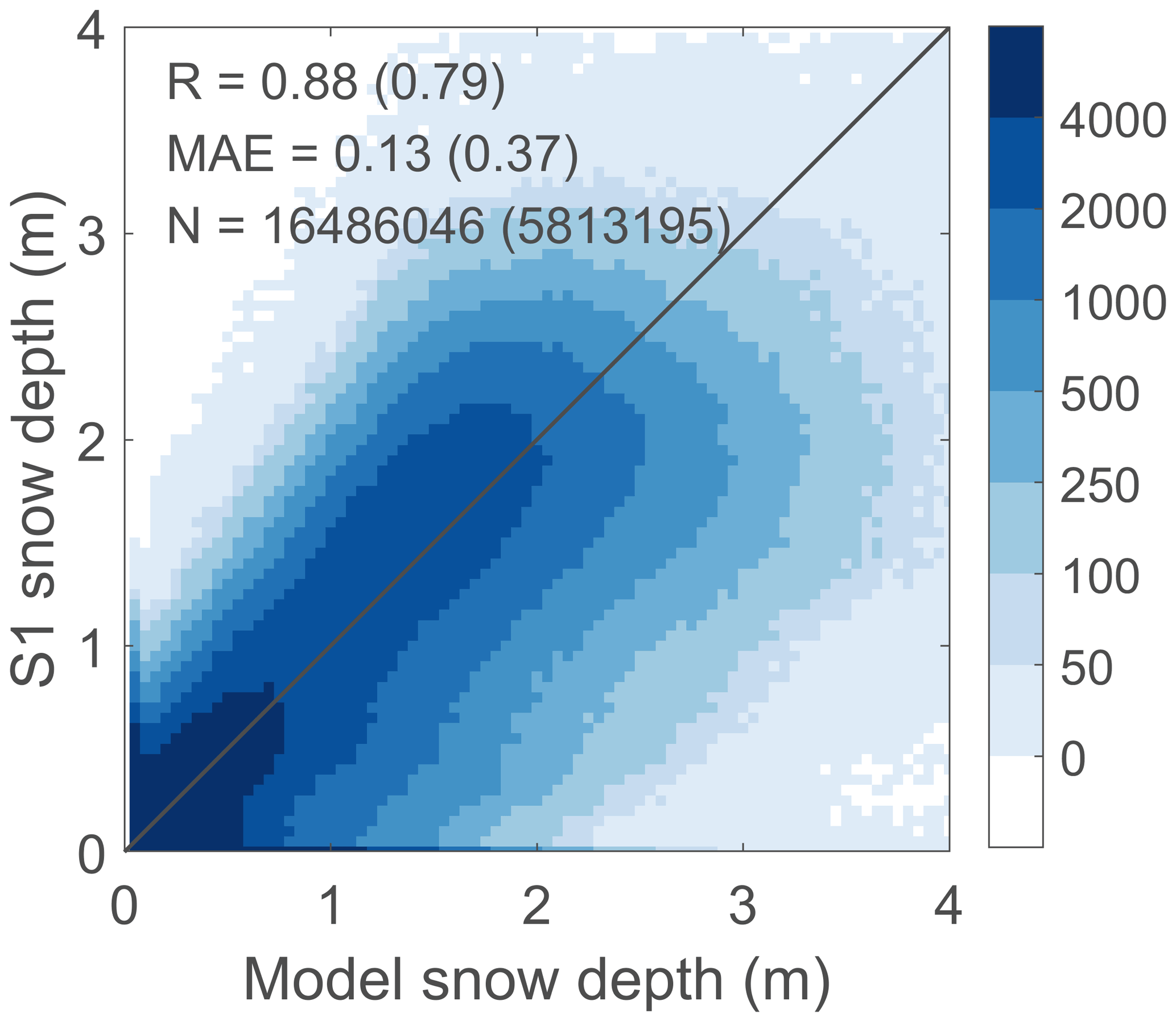
Figure 9Density plot comparing 1 km S1 retrievals of snow depth (m) with corresponding model simulations (m) for August through April 2017–2018 and 2018–2019 (wet snow excluded). The spatio-temporal Pearson correlation R (–), the MAE (m), and number of observations (N) are shown at the top left, for scenarios both with and (between brackets) without the inclusion of zero values.
Finally, the dry snow depth retrievals from S1 at 1 km resolution are compared against the corresponding model simulations for August through April 2017–2018 and 2018–2019 in Fig. 9. The density plot comprises more than 16 million data pairs, which reduces to ∼5.8 million if zero snow depths are excluded. The spatio-temporal correlation between the simulations and retrievals is 0.88 (0.79 with zero depths excluded), and the MAE is 0.13 m (0.37 m). The density plot indicates a slightly more frequent occurrence of underestimation in S1 snow depth as opposed to overestimation. This can for instance be due to (i) undetected wet snow that decreases the backscatter or (ii) above-snow vegetation that reduces the sensitivity of backscatter to snow but also (iii) uncertainties in the model simulations. Nevertheless, the results overall demonstrate that the S1 retrievals represent the spatio-temporal distribution of the snow depth simulations well.
3.2 Validation of S1 retrievals with in situ measurements
Figure 10 shows examples of S1 retrievals of snow depth and snow state (dry or wet) over the Alps at 500 m spatial resolution for three dates: 8 November 2017, 29 January 2018, and 18 February 2019. The S1 retrievals for instance capture the strong increase in snow depth during winter 2017–2018 (Fig. 10a and c). The Alps experienced several episodes of extreme snowfall in January 2018, caused by a low-pressure system over the western Mediterranean that brought moist air northwards and resulted in an anomalously deep snowpack. The winter 2018–2019 was generally warmer than average, caused by a persistent high-pressure system over western Europe. The warm temperatures led to extensive wet snow conditions during February that were detected by S1 (Fig. 10f) and can be used for masking the corresponding snow depth retrievals. Unlike in the northern Alps, where wet snow occurrence is widespread on 18 February 2019, wet snow is mostly limited to the valleys of the southern Alps.
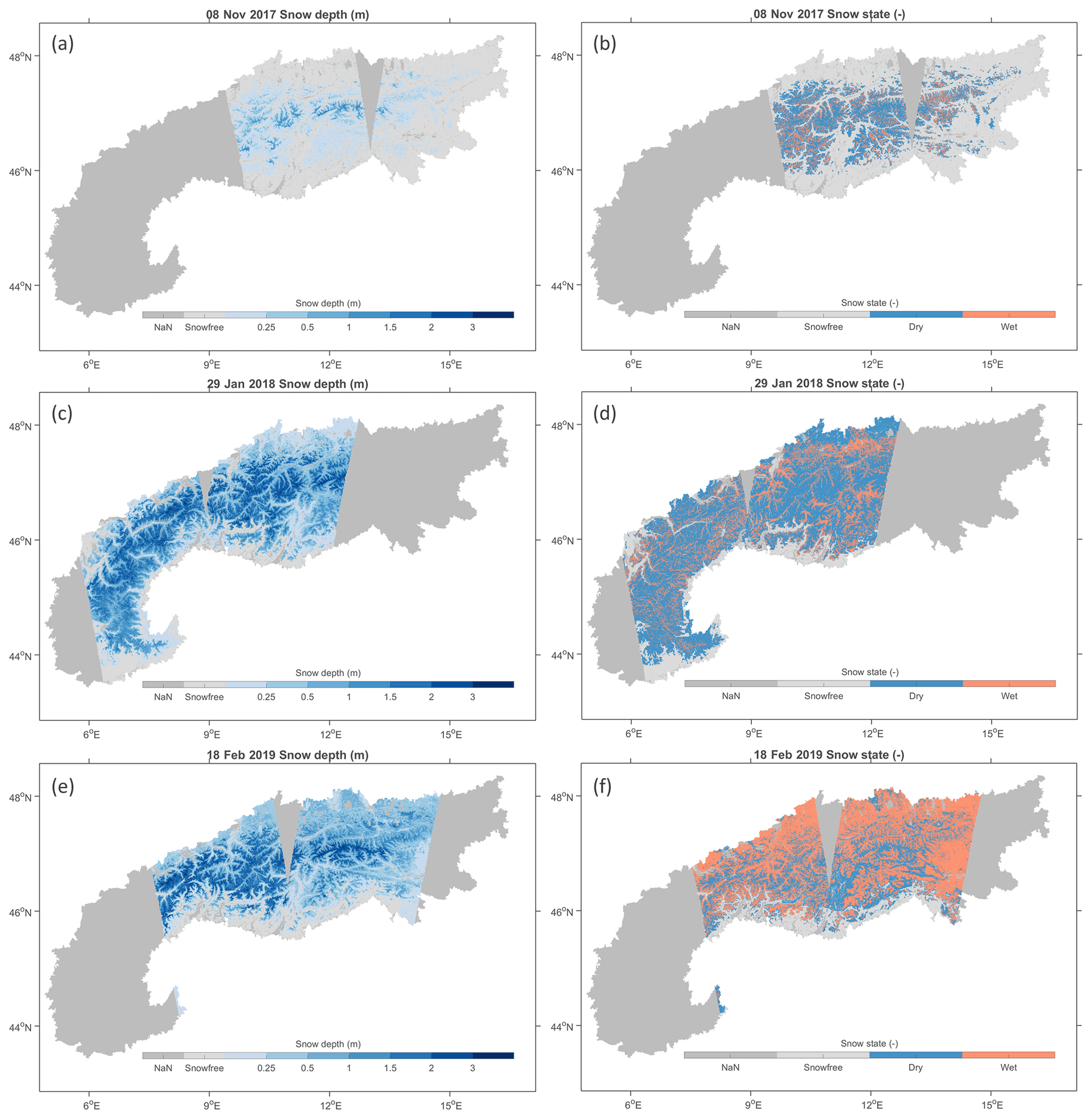
Figure 10S1 snow depth (m) and snow state (dry or wet) retrievals at 500 m spatial resolution over the Alps, for (a, b) 8 November 2017, (c, d) 29 January 2018, and (e, f) 18 February 2019.
In Fig. 11, the S1 snow depth retrievals at the three different spatial resolutions (100 m, 500 m, and 1 km) are compared against independent point-scale in situ measurements over the periods August through April 2017–2018 and 2018–2019, both with and without wet snow masking. Although the more detailed retrievals at the finer 100 m resolution have the potential to better represent the local point-scale conditions at the in situ sites, a higher accuracy is obtained at the coarser 500 m and 1 km resolutions. The lower accuracy for the finer-scale retrievals can be caused by the larger impacts of (i) radar speckle that is inherent to radar measurements; (ii) geolocation errors and geometric distortions (foreshortening, layover) in the radar images causing location mismatches in γ0 time series; and (iii) local heterogeneity in topography (elevation, slope, aspect), land surface properties (land cover, soil moisture, soil temperature, and surface roughness), and snow variables (stratigraphy and microstructure). The 500 m retrievals offer a potential balance between resolution and accuracy. The resolution is sufficiently high to capture the high spatial variability in snow depth at the hill-slope scale, while the accuracy (spatio-temporal R=0.89, MAE = 0.18 m, for dry snow) is comparable to that of the coarser 1 km scale (R=0.89, MAE = 0.17 m). However, the resolution requirement may depend on the envisaged application. For instance, the 1 km resolution may be too coarse for operational water management but more than sufficient for regional numerical weather prediction.
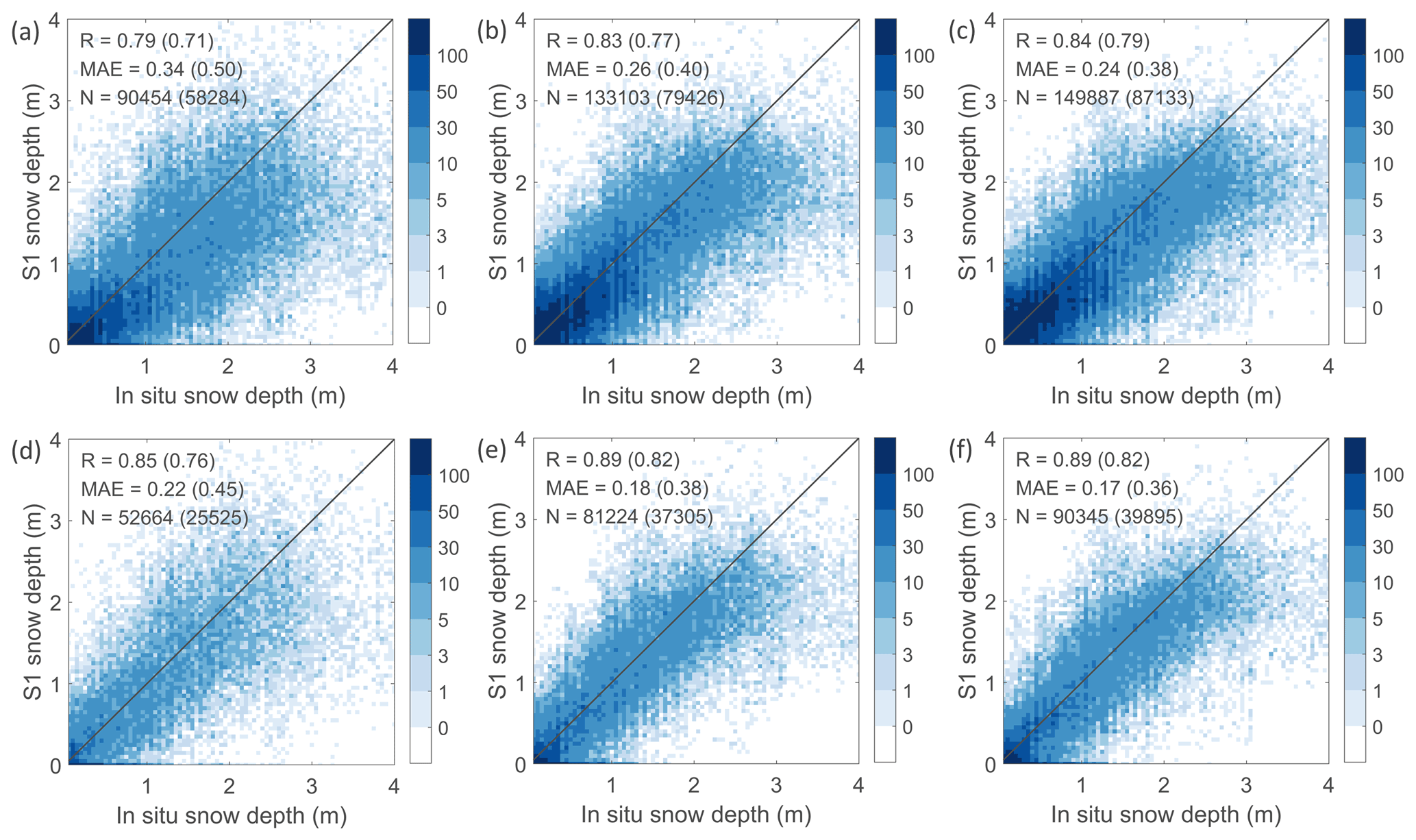
Figure 11Density plots comparing S1 retrievals of snow depth (m) with corresponding in situ measurements (m) for August through April 2017–2018 and 2018–2019. The comparison is shown for retrievals at (a, d) 100 m, (b, e) 500 m, and (c, f) 1 km resolution, with (a–c) excluding wet snow masking and (d–f) including wet snow masking. The spatio-temporal Pearson correlation R (–), the MAE (m), and number of observations (N) are shown at the top left, for scenarios both with and (between brackets) without the inclusion of zero values.
Figure 12 shows the temporal correlation and spatial correlation between the S1 retrievals and in situ measurements of snow depth, stratified by the range of the in situ measurements. In agreement with the comparison against model simulations (Sect. 3.1), the temporal correlation increases with the snow depth range, reaching consistently high values (>0.8) for sites with snow depths reaching above 1 m. Similarly, the spatial correlation increases with increasing snow depth range, reaching values of ∼0.6–0.8 when snow depths above 1 m are included.
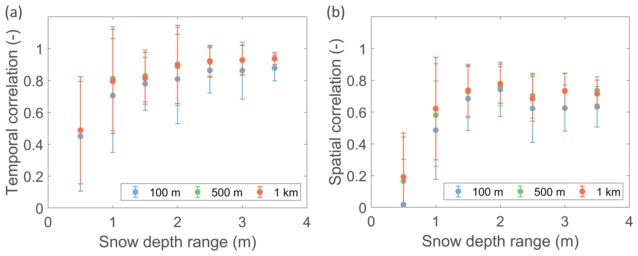
Figure 12The (a) temporal and (b) spatial correlation between 100 m, 500 m, and 1 km S1 retrievals and in situ measurements for August through April 2017–2018 and 2018–2019. Zero snow depths and wet snow detected by S1 are excluded. The metrics are stratified by the snow depth range (or maximum) of the in situ measurements and represent the mean value and standard deviation per 0.5 m interval. Note that for the temporal correlation, the mean and standard deviation are calculated from different locations in space, whereas for the spatial correlation, the metrics are calculated from different time steps.
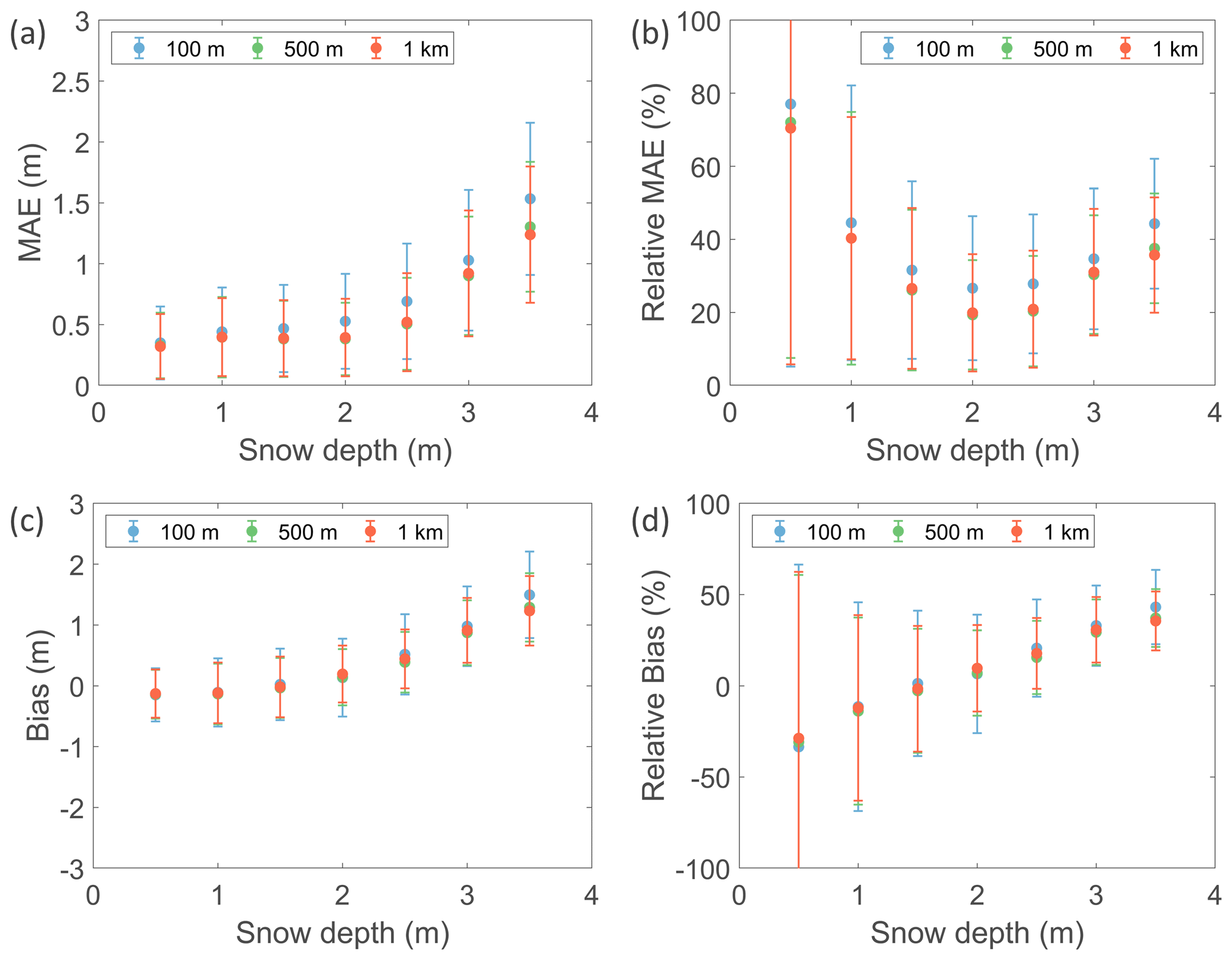
Figure 13The (a) MAE (m), (b) relative MAE (%), (c) bias (m), and (d) relative bias (%) between 100 m, 500 m, and 1 km S1 retrievals and in situ measurements for August through April 2017–2018 and 2018–2019. Bars indicate ±1 standard deviation. Wet snow detected by S1 is excluded. The metrics are stratified by the measured snow depth value (not by the range as in Fig. 12), with intervals of 0.5 m.
Figure 13 shows the MAE and bias (measurements minus retrievals), as both absolute values and relative values to the measured snow depth. The MAE remains relatively constant around 0.3–0.4 m for snow depths of 0.5–2 m, followed by an increase for deeper snow towards ∼1.3 m at 3.5 m depth. The relative MAE ranges between 20 % and 30 % for snow depths of 1.5–3 m and is larger for shallower (40 %–70 %) and deeper (∼40 %) snow. The absolute bias indicates a minor overestimation by S1 for shallow snow. However, the corresponding relative biases for shallow snow can be large (up to ∼30 %) due to the low reference measurements. The bias reduces with increasing snow depth to result in bias-free estimates at 1.5–2 m depths. Deeper snow is increasingly underestimated, reaching ∼1.2 m bias at 3.5 m depth (35 %). A caveat to the assessment is that only few measurements are available for snow depths above 3 m. Furthermore, part of the biases (and errors) can be due to the scaling of the retrievals based on model simulations and not based on in situ measurements (see Sect. 2.2). Indeed, the model simulations also show a very similar underestimation of the high snow depth measurements (data not shown). Furthermore, part of the biases and errors can be due to representativeness differences between the point-scale in situ measurements and the grid-scale satellite retrievals. For instance, in situ sites typically correspond with open flat field locations and often overestimate the mean snow depth of the surrounding terrain (Grünewald and Lehning, 2015). Intuitively, one would expect an improvement in skill for retrievals at a finer spatial scale (e.g., 100 m), although statistically, it can be proven that fine-scale errors are reduced after aggregation to coarser-scale estimates. Our results show that the skill improves with coarser scales, although more when retrievals are aggregated from 100 to 500 m than from 500 m to 1 km. In general, this indicates that the potential improvement brought by the finer spatial scale of the retrieval can be offset by an increase in noise. In order to investigate the impacts of representativeness differences, future research is recommended to compare the S1 snow depth retrievals with validation data at the matching scale, such as snow depth estimates from lidar.
Sentinel-1 (S1) backscatter observations, particularly in VH polarization, correlate well with regional model simulations of snow depth over Austria and Switzerland. Using a combination of cross-polarized and co-polarized backscatter as input to an empirical orbit-dependent change detection algorithm, S1 snow depth retrievals at 100 m, 500 m, and 1 km spatial and less-than-weekly temporal resolution are presented over the European Alps for the periods from August through April 2017–2019. The accuracy of the retrievals is validated using independent local time series measurements of snow depth at 743 locations across the Alps. Despite the typically large representativeness differences between these point-scale in situ measurements and grid-scale satellite retrievals, good skill metrics are obtained. At 500 m and 1 km resolutions and for dry snow conditions, the spatio-temporal Pearson correlation coefficient equals 0.89, and the relative mean absolute error ranges between ∼20 %–30 % for snow depths between 1.5 and 3 m. A slightly lower accuracy is observed at 100 m resolution, which is likely caused by increased impacts of measurement noise; geolocation errors and geometric distortions; and the local heterogeneity in topography, land surface, and snow properties, such as microstructure and stratigraphy.
The main uncertainties in the S1 snow depth retrievals are expected to be caused by wet, shallow, and occasional snow cover and forest cover. Wet snow is known to cause a strong decrease in radar backscatter due to signal absorption. Although a wet snow detection algorithm is implemented, undetected wet snow (for instance due to an insufficient decrease in the backscatter) may cause underestimation in the snow depth retrievals. Uncertainties can also be large in regions with shallow and occasional snow cover, where the backscatter observations can be dominated by scattering contributions from the ground surface, resulting in a weak (or even negative) correlation with snow depth. For shallow snow conditions, backscatter observations at higher frequencies (e.g., X- or Ku-band) or potentially also using InSAR phase changes at lower (e.g., L- or P-band) frequencies could be more suitable to detect short-term snow depth changes. Higher uncertainties in the S1 retrievals may also be found in regions with large open-water (lake) areal coverage and in densely forested regions, where the attenuation of the radar signal may reduce the sensitivity to snow. The comparison of S1 retrievals with regional model simulations of snow depth reveals that sensitivity is generally strong (e.g., time series correlations >0.8) if the maximum snow depth reaches above ∼1 m at an elevation above ∼1000 m or with a forest cover fraction below ∼80 %.
The S1 retrievals can provide important information on the spatial distribution of snow depth in regions with complex topography, which are typically excluded in passive microwave retrievals. Therefore, the results of this study may contribute to improving our knowledge on the terrestrial snow mass budget. An asset of the approach is the confirmed long-term availability of S1 observations, with continuity by S1C and S1D over the coming decades. This will allow for the generation of long time series that are required for investigating the potential impacts of climate variability or climate change on snow mass in mountain regions and for assessing the corresponding impacts on water availability to society. Finally, the combination of the S1 retrievals with land surface model estimates through data assimilation is expected to be rewarding. Not only could the assimilation ensure improved and continuous (in time and space) estimates of mountain snow mass, it is also likely to benefit associated applications such as operational water management, natural hazard (avalanche and flood) prediction, or numerical weather prediction.
Further research is needed to investigate the physical basis of C-band radar backscatter sensitivity to snow, for instance based on tower radar measurements and corresponding detailed measurements of snowpack properties, including snow microstructure and stratigraphy. Also, future research is recommended to investigate the validation of the S1 snow depth retrievals using data at the matching scale, for instance from lidar, and to further investigate the performance of the approach in other regions with different soil substrate types, vegetation conditions, and snow climate conditions.
The Sentinel-1 snow depth retrievals at 500 m and 1 km spatial and less-than-weekly temporal resolution are available online at https://ees.kuleuven.be/project/c-snow (Lievens et al., 2021).
HL, IB, HPM, and GDL contributed to the Sentinel-1 snow depth retrieval algorithm. HL performed the analysis. TJ and MO produced the snow model simulations and provided in situ measurements. All co-authors contributed to the writing of the manuscript.
The contact author has declared that neither they nor their co-authors have any competing interests.
Publisher's note: Copernicus Publications remains neutral with regard to jurisdictional claims in published maps and institutional affiliations.
Sentinel-1A/B data are from the ESA and Copernicus Sentinel Satellites project and were processed using the ESA Sentinel Application Platform (SNAP). The resources and services used in this work were provided by the VSC (Flemish Supercomputer Center), funded by the Research Foundation – Flanders (FWO) and the Flemish Government.
This research has been supported by the BELSPO C-SNOW project (contract SR/01/375).
This paper was edited by Chris Derksen and reviewed by two anonymous referees.
Arslan, A. N., Pulliainen, J., and Hallikainen, M.: Observations of L-and C-band backscatter and a semi-empirical backscattering model approach from a forest-snow-ground system, Prog. Electromagn. Res., 56, 263–281, 2006. a, b
Baghdadi, N., Gauthier, Y., and Bernier, M.: Capability of multitemporal ERS-1 SAR data for wet snow mapping, Remote Sens. Environ., 60, 174–186, 1997. a, b, c
Bernier, M. and Fortin, J.-P.: The potential of times series of C-band SAR data to monitor dry and shallow snow cover, IEEE T. Geosci. Remote, 36, 226–243, 1998. a, b
Bernier, M., Fortin, J.-P., Gauthier, Y., Gauthier, R., Roy, R., and Vincent, P.: Determination of snow water equivalent using RADARSAT SAR data in eastern Canada, Hydrol. Process., 13, 3041–3051, 1999. a
Blöschl, G.: Scaling issues in snow hydrology, Hydrol. Process., 13, 2149–2175, 1999. a
Bormann, K. J., Brown, R. D., Derksen, C., and Painter, T. H.: Estimating snow-cover trends from space, Nat. Clim. Change, 8, 924–928, 2018. a, b
Buchhorn, M., Smets, B., Bertels, L., De Roo, B., Lesiv, M., Tsendbazar, N.-E., Herold, M., and Fritz, S.: Copernicus Global Land Service: Land Cover 100 m: collection 3: epoch 2018: Globe 2020, Zenodo, https://doi.org/10.5281/zenodo.3939050, 2020. a
Chang, W., Tan, S., Lemmetyinen, J., Tsang, L., Xu, X., and Yueh, S. H.: Dense media radiative transfer applied to SnowScat and SnowSAR, IEEE J. Sel. Top. Appl., 7, 3811–3825, 2014. a, b
Conde, V., Nico, G., Mateus, P., Catalão, J., Kontu, A., and Gritsevich, M.: On the estimation of temporal changes of snow water equivalent by spaceborne SAR interferometry: a new application for the Sentinel-1 mission, J. Hydrol. Hydromech., 67, 93–100, 2019. a
Dechant, C. and Moradkhani, H.: Radiance data assimilation for operational snow and streamflow forecasting, Adv. Water Resour., 34, 351–364, 2011. a
de Rosnay, P., Balsamo, G., Albergel, C., Muñoz-Sabater, J., and Isaksen, L.: Initialisation of land surface variables for numerical weather prediction, Surv. Geophys., 35, 607–621, 2014. a
Dozier, J., Bair, E. H., and Davis, R. E.: Estimating the spatial distribution of snow water equivalent in the world's mountains, WIREs Water, 3, 461–474, 2016. a, b
Du, J., Shi, J., and Rott, H.: Comparison between a multi-scattering and multi-layer snow scattering model and its parameterized snow backscattering model, Remote Sens. Environ., 114, 1089–1098, 2010. a, b
Essery, R., Morin, S., Lejeune, Y., and Ménard, C. B.: A comparison of 1701 snow models using observations from an alpine site, Adv. Water Resour., 55, 131–148, 2013. a
Foster, J. L., Sun, C., Walker, J. P., Kelly, R., Chang, A., Dong, J., and Powell, H.: Quantifying the uncertainty in passive microwave snow water equivalent observations, Remote Sens. Environ., 94, 187–203, 2005. a
Frey, S. and Holzmann, H.: A conceptual, distributed snow redistribution model, Hydrol. Earth Syst. Sci., 19, 4517–4530, https://doi.org/10.5194/hess-19-4517-2015, 2015. a
Gelaro, R., McCarty, W., Suárez, M. J., Todling, R., Molod, A., Takacs, L., Randles, C. A., Darmenov, A., Bosilovich, M. G., Reichle, R., Wargan, K., Coy, L., Cullather, R., Draper, C., Akella, S., Buchard, V., Conaty, A., Da Silva, A. M., Gu, W., Kim, G.-K., Koster, R., Lucchesi, R., Merkova, D., Nielsen, J. E., Partyka, G., Pawson, S., Putman, W., Rienecker, M., Schubert, S. D., Sienkiewicz, M., and Zhao, B.: The Modern-Era Retrospective Analysis for Research and Applications, Version 2 (MERRA-2), J. Climate, 30, 5419–5454, 2017. a
Girotto, M., Musselman, K. N., and Essery, R. L. H.: Data assimilation improves estimates of climate-sensitive seasonal snow, Current Climate Change Reports, 6, 81–94, 2020. a
Griessinger, N., Schirmer, M., Helbig, N., Winstral, A., Michel, A., and Jonas, T.: Implications of observation-enhanced energy-balance snowmelt simulations for runoff modeling of Alpine catchments, Adv. Water Resour., 133, 103410, https://doi.org/10.1016/j.advwatres.2019.103410, 2019. a
Grünewald, T. and Lehning, M.: Are flat-field snow depth measurements representative? A comparison of selected index sites with areal snow depth measurements at the small catchment scale, Hydrol. Process., 29, 1717–1728, 2015. a, b, c
Guneriussen, T., Høgda, K. A., Johnsen, H., and Lauknes, I.: InSAR for estimation of changes in snow water equivalent of dry snow, IEEE T. Geosci. Remote, 41, 230–242, 2001. a
Haslinger, K. and Bartsch, A.: Creating long-term gridded fields of reference evapotranspiration in Alpine terrain based on a recalibrated Hargreaves method, Hydrol. Earth Syst. Sci., 20, 1211–1223, https://doi.org/10.5194/hess-20-1211-2016, 2016. a
Helbig, N., van Herwijnen, A., Magnusson, J., and Jonas, T.: Fractional snow-covered area parameterization over complex topography, Hydrol. Earth Syst. Sci., 19, 1339–1351, https://doi.org/10.5194/hess-19-1339-2015, 2015. a
Hiebl, J. and Frei, C.: Daily temperature grids for Austria since 1961 – concept, creation and applicability, Theor. Appl. Climatol., 124, 161–178, 2016. a
Hiebl, J. and Frei, C.: Daily precipitation grids for Austria since 1961 – development and evaluation of a spatial dataset for hydro-climatic monitoring and modelling, Theor. Appl. Climatol., 132, 327–345, 2018. a
Immerzeel, W. W., Lutz, A. F., Andrade, M., Bahl, A., Biemans, H., Bolch, T., Hyde, S., Brumby, S., Davies, B. J., Elmore, A. C., Emmer, A., Feng, M., Fernández, A., Haritashya, U., Kargel, J. S., Koppes, M., Kraaijenbrink, P. D. A., Kulkarni, A. V., Mayewski, P. A., Nepal, S., Pacheco, P., Painter, T. H., Pellicciotti, F., Rajaram, H., Rupper, S., Sinisalo, A., Shrestha, A. B., Viviroli, D., Wada, Y., Xiao, C., Yao, T., and Baillie, J. E. M.: Importance and vulnerability of the world's water towers, Nature, 577, 364–369, 2020. a
Kelly, R. E., Chang, A. T., Tsang, L., and Foster, J. L.: A prototype AMSR-E global snow area and snow depth algorithm, IEEE T. Geosci. Remote, 41, 230–242, 2003. a
King, J., Kelly, R., Kasurak, A., Duguay, C., Gunn, G., Rutter, N., Watts, T., and Derksen, C.: Spatio-temporal influence of tundra snow properties on Ku-band (17.2 GHz) backscatter, J. Glaciol., 61, 267–279, 2015. a
Leinss, S., Wiesmann, A., Lemmetyinen, J., and Hajnsek, I.: Snow water equivalent of dry snow measured by differential interferometry, IEEE J. Sel. Top. Appl., 8, 3773–3790, 2015. a
Leinss, S., Löwe, H., Proksch, M., Lemmetyinen, J., Wiesmann, A., and Hajnsek, I.: Anisotropy of seasonal snow measured by polarimetric phase differences in radar time series, The Cryosphere, 10, 1771–1797, https://doi.org/10.5194/tc-10-1771-2016, 2016. a
Lemmetyinen, J., Derksen, C., Rott, H., Macelloni, G., King, J., Schneebeli, M., Wiesmann, A., Leppänen, L., Kontu, A., and Pulliainen, J.: Retrieval of effective correlation length and snow water equivalent from radar and passive microwave measurements, Remote Sens.-Basel, 10, 170, https://doi.org/10.3390/rs10020170, 2018. a
Lievens, H., Demuzere, M., Marshall, H. P., Reichle, R. H., Brucker, L., and co-authors: Snow depth variability in the Northern Hemisphere mountains observed from space, Nat. Commun., 10, 4629, https://doi.org/10.1038/s41467-019-12566-y, 2019. a, b, c, d, e
Lievens, H., Brangers, I., Marshall, H.-P., De Lannoy, G. J. M.: Sentinel-1 snow depth retrievals at 500 m and 1 km spatial resolution over the European Alps for August through April 2017–2018 and 2018–2019, https://ees.kuleuven.be/project/c-snow, last access: 8 December 2021. a
Luojus, K. P., Pulliainen, J., Metsamaki, S., and Hallikainen, M.: Snow-covered area estimation using satellite radar wide-swath images, IEEE T. Geosci. Remote, 45, 978–989, 2007. a, b
Magnusson, J., Gustafsson, D., Hüsler, F., and Jonas, T.: Assimilation of point SWE data into a distributed snow cover model comparing two contrasting methods, Water Resour. Res., 50, 7816–7835, 2014. a
Manickam, S. and Barros, A.: Parsing synthetic aperture radar measurements of snow in complex terrain: scaling behaviour and sensitivity to snow wetness and landcover, Remote Sens.-Basel, 12, 483, https://doi.org/10.3390/rs12030483, 2020. a, b, c
Marin, C., Bertoldi, G., Premier, V., Callegari, M., Brida, C., Hürkamp, K., Tschiersch, J., Zebisch, M., and Notarnicola, C.: Use of Sentinel-1 radar observations to evaluate snowmelt dynamics in alpine regions, The Cryosphere, 14, 935–956, https://doi.org/10.5194/tc-14-935-2020, 2020. a, b
Meromy, L., Molotch, N. P., Link, T. E., Fassnacht, S. R., and Rice, R.: Subgrid variability of snow water equivalent at operational snow stations in the western USA, Hydrol. Process., 27, 2383–2400, 2013. a
Nagler, T. and Roth, H.: Retrieval of wet snow by means of multitemporal SAR data, IEEE T. Geosci. Remote, 38, 754–765, 2000. a, b
Nagler, T., Roth, H., Ripper, E., Bippus, G., and Hetzenecker, M.: Advancements for snowmelt monitoring by means of Sentinel-1 SAR, Remote Sens.-Basel, 8, 348, https://doi.org/10.3390/rs8040348, 2016. a, b, c
National Ice Center: IMS daily Northern Hemisphere snow and ice analysis at 1 km, 4 km, and 24 km resolutions, National Snow and Ice Data Center, Boulder, CO, Digital media, https://doi.org/10.7265/N52R3PMC, 2008. a
Niu, G.-Y, Yang, Z.-L., Mitchell, K. E., Chen, F., Ek, M. B., Barlage, M., Kumar, A., Manning, K., Niyogi, D., Rosero, E., Tewari, M., and Xia, Y.: The community Noah land surface model with multiparameterization options (Noah-MP): 1. Model description and evaluation with local-scale measurements, J. Geophys. Res., 116, D12109, https://doi.org/10.1029/2010JD015139, 2011. a
Olefs, M., Koch, R., Schöner, W., and Marke, T.: Changes in snow depth, snow cover duration, and potential snowmaking conditions in Austria, 1961–2020 – A model based approach, Atmosphere, 11, 1330, https://doi.org/10.3390/atmos11121330, 2020. a, b
Pellicciotti, F., Brock, B., Strasser, U., Burlando, P., Funk, M., and Corripio, J.: An enhanced temperature-index glacier melt model including the shortwave radiation balance: development and testing for Haut Glacier d'Arolla, Switzerland, J. Glaciol., 51, 573–587, 2005. a
Pivot, F.: C-Band SAR imagery for snow-cover monitoring at treeline, Churchill, Manitoba, Canada, Remote Sens.-Basel, 4, 2133–2155, 2012. a, b
Pulliainen, J., Luojus, K., Derksen, C., Mudryk, L., Lemmetyinen, J., Salminen, M., Ikonen, J., Takala, M., Cohen, J., Smolander, T., and Norberg, J.: Patterns and trends of Northern Hemisphere snow mass from 1980 to 2018, Nature, 581, 294–298, 2020. a
RGI Consortium: Randolph Glacier Inventory – A Dataset of Global Glacier Outlines: Version 6.0, Global Land Ice Measurements from Space, RGI, Colorado, USA [data set], https://doi.org/10.7265/N5-RGI-60, 2017. a
Rott, H. and Nagler, T.: Capabilities of ERS-1 SAR for snow and glacier monitoring in alpine areas, in: Proceedings of the Second ERS-1 Symposium, 11–14 October 1993, Hamburg, Germany, 1–6, 1993. a, b
Rott, H., Yueh, S. H., Cline, D. W., Duguay, C., Essery, R., Haas, C., Hélière, F., Kern, M., Macelloni, G., Malnes, E., Nagler, T., Pulliainen, J., Rebhan, H., and Thompson, A.: Cold regions hydrology high-resolution observatory for snow and cold land processes, Proc. IEEE, 98, 752–765, 2010. a
Schattan, P., Baroni, G., Oswald, S. E., Schöber, J., Fey, C., Kormann, C., Huttenlau, M., and Achleitner, S.: Continuous monitoring of snowpack dynamics in alpine terrain by aboveground neutron sensing, Water Resour. Res., 53, 3615–3634, 2017. a
Seidel, F. C., Rittger, K., Skiles, S. M., Molotch, N. P., and Painter, T. H.: Case study of spatial and temporal variability of snow cover, grain size, albedo and radiative forcing in the Sierra Nevada and Rocky Mountain snowpack derived from imaging spectroscopy, The Cryosphere, 10, 1229–1244, https://doi.org/10.5194/tc-10-1229-2016, 2016. a
Shi, J. and Dozier, J.: Estimation of snow water equivalence using SIR-C/X-SAR, part II: Inferring snow depth and particle size, IEEE T. Geosci. Remote, 38, 2475–2488, 2000. a, b, c
Small, D.: Flattening gamma: radiometric terrain correction for SAR imagery, IEEE T. Geosci. Remote, 49, 3081–3093, 2011. a
Small, D., Rohner, C., Miranda, N., Rüetschi, M., and Schaepman, M. E.: Wide-area analysis-ready radar backscatter composites, IEEE T. Geosci. Remote, 60, 5201814, https://doi.org/10.1109/TGRS.2021.3055562, 2022. a
Takala, M., Luojus, K., Pulliainen, J., Derksen, C., Lemmetyinen, J., Kärnä, J. P., Koskinen, J., and Bojkov, B.: Estimating Northern Hemisphere snow water equivalent for climate research through assimilation of spaceborne radiometer data and ground-based measurements, Remote Sens. Environ., 115, 3517–3529, 2011. a
Tedesco, M. and Narvekar, P. S.: Assessment of the NASA AMSR-E SWE Product, IEEE J. Sel. Top. Appl., 3, 141–159, 2010. a
Tsai, Y.-L. S., Dietz, A., Oppelt, N., and Kuenzer, C.: Wet and dry snow detection using Sentinel-1 SAR data for mountainous areas with a machine learning technique, Remote Sens.-Basel, 11, 895, https://doi.org/10.3390/rs11080895, 2019. a, b
Vreugdenhil, M., Navacchi, C., Bauer-Marschallinger, B., Hahn, S., Steele-Dunne, S., Pfeil, I., Dorigo, W., and Wagner, W.: Sentinel-1 cross ratio and vegetation optical depth: A comparison over Europe, Remote Sens.-Basel, 12, 3404, https://doi.org/10.3390/rs12203404, 2020. a
Winstral, A., Magnusson, J., Schirmer, M., and Jonas, T.: The bias-detecting ensemble: A new and efficient technique for dynamically incorporating observations into physics-based, multi-layer snow models, Water Resour. Res., 55, 613–631, 2019. a, b
Yueh, S. H., Dinardo, S. J., Akgiray, A., West, R., Cline, D. W., and Elder, K.: Airborne Ku-band polarimetric radar remote sensing of terrestrial snow cover, IEEE T. Geosci. Remote, 47, 3347–3364, 2009. a
Zemp, M., Huss, M., Thibert, E., Eckert, N., McNabb, R., and co-authors: Global glacier mass changes and their contributions to sea-level rise from 1961 to 2016, Nature, 568, 382–386, 2019. a