Brief communication: Estimating the ice thickness of the Müller Ice Cap to support selection of a drill site

The Müller Ice Cap will soon set the scene for a new drilling project. Therefore, ice thickness estimates are necessary for planning, since thickness measurements of the ice cap are sparse. Here, three models are presented and compared: (i) a simple Semi-Empirical Ice Thickness Model (SEITMo) based on an inversion of the shallow-ice approximation by the use of a single radar line in combination with the glacier outline, surface slope, and elevation; (ii) an iterative inverse method using the Parallel Ice Sheet Model (PISM), and (iii) a velocity-based inversion of the shallow-ice approximation. The velocity-based inversion underestimates the ice thickness at the ice cap top, making the model less useful to aid in drill site selection, whereas PISM and the SEITMo mostly agree about a good drill site candidate. However, the new SEITMo is insensitive to mass balance, computationally fast, and provides as good fits as PISM.

1 Introduction

The Müller Ice Cap (MIC), located on Axel Heiberg Island in Arctic Canada, is facing the Arctic Ocean, where no full depth ice core has been drilled to date, making it an interesting drill site location. Choosing a good drill site location with stratified ice layers, a good time resolution, and a good age span is crucial in the dating process needed to interpret the different compounds in the ice and to put it into a climatological context. However, the MIC remains poorly studied with the exception of a few mass balance (Koerner, 1979; Thomson et al., 2011) and surface velocity (van Wychen et al., 2014) studies, leaving the ice thickness poorly constrained. Therefore, knowledge about ice thickness and flow is important as thick ice and minimal horizontal flow are desirable to increase the probability of reaching ice that stems from the Innuitian ice sheet, referring to the ice sheet located between the Laurentide and Greenland ice sheets during the last glaciation. This limited knowledge stands in contrast to one of its neighbouring glaciers, White Glacier, marked in Fig. 1. White Glacier has been studied thoroughly since the late 1960s (Müller, 1962; Cogley et al., 1996, 2011) with a strong focus on the mass balance. To ensure a good drill site, ground-based radar measurements are necessary. However, fieldwork constraints make it impractical and expensive to survey the entire ice cap, and it is therefore necessary to be selective when deciding where to conduct ground-based radar measurements.

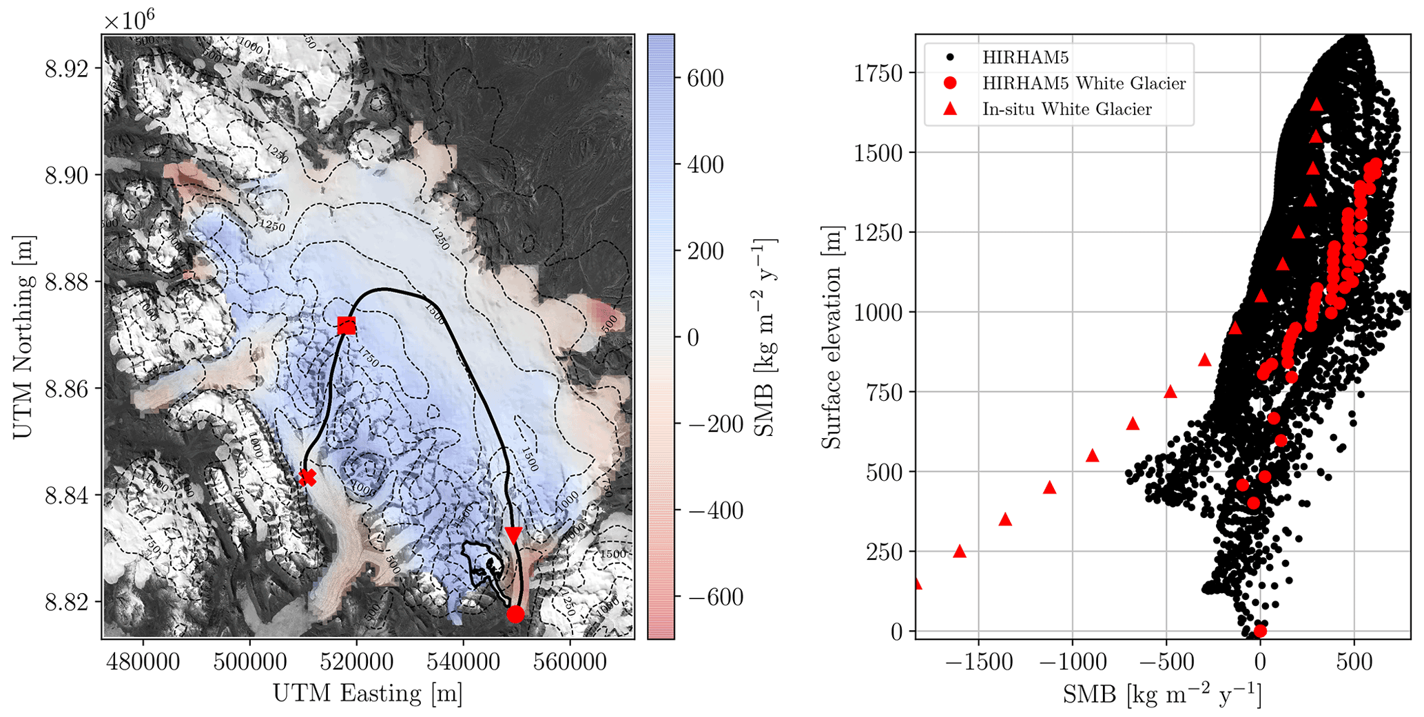
Figure 1 Left: Landsat 8 satellite image of the Müller Ice Cap overlaid with long-term average HIRHAM5 surface mass balance (SMB) from 1980–2016. Contour lines of surface elevation from ArcticDEM with 250 m increments, and the Operation IceBridge flight line as the solid black line from the red dot to the red cross. The four red symbols have the same location as in Fig. 3 and are present to guide the reader. White Glacier is outlined in black just above the red dot. The coordinates are given in UTM zone 15N. Right: surface mass balance as a function of surface elevation. Red triangles are average in situ measurements from White Glacier from 1960–91 (Cogley et al., 1996). The black and red dots are long-term HIRHAM5 SMB averages from 1980–2016, with the red dots corresponding to the SMB within the White Glacier polygon.

The Ice Thickness Models Intercomparison eXperiment phases 1 and 2, ITMIX1 (Farinotti et al., 2017) and ITMIX2 (Farinotti et al., 2021), compare various models that estimate the ice thicknesses of glaciers and ice caps from sparse data. In ITMIX1, large differences are found between the models on ice caps in the vicinity of ice divides. Furthermore, it is urged that modellers seek improvements on how to treat these regions to ensure continuity of the subsurface topography around the ice divide. In this study, it is of particular importance that we resolve the area around the ice divide well, as ice divides often qualify as good drill site locations due to limited horizontal ice flow. Furthermore, from ITMIX1 it is not possible to determine what model approaches are to be preferred on ice caps. Thus, to narrow down areas of conducting ground-based radar measurements, the ice thickness is modelled using three different techniques that differ greatly in computational demands, input data, and model setup. One is a simple Semi-Empirical Ice Thickness Model (SEITMo) based on the shallow-ice approximation (SIA; Hutter, 1983), only relying on the surface elevation, the ice cap outline, and a single Operation IceBridge (OIB) (Paden et al., 2010) flight line with thickness measurement. This is a fast new method that differs from existing SIA approaches due to its semi-empirical nature which makes it less sensitive to mass balance, steady-state assumptions, and ice flow physics. The second is an iterative inverse method using the Parallel Ice Sheet Model (PISM) as a forward model, which has to be forced with both climate data and an initial guess of ice cap geometry. The third is a velocity-based inversion of the SIA as presented in Zorzut et al. (2020), henceforth referred to as Zorzut. This method is similar to the one used in the recently published global glacier thickness estimate (Millan et al., 2022). Zorzut relies on the surface velocity and slope, alongside an OIB flight line of ice thickness measurements as for the SEITMo.

2 Data

Ice thickness measurements taken from the Multichannel Coherent Radar Depth Sounder from OIB (Paden et al., 2010) are used to validate all models and to invert the two SIA-based methods, SEITMo and Zorzut. Only two flight lines cross the top of the ice cap, and since the tracks of those flight lines are practically identical, only the newest one acquired on 30 March 2017 is used (Fig. 1).

The surface elevation is obtained from the Arctic Digital Elevation Model (ArticDEM; Porter et al., 2018) and is shown as contours in Fig. 1. To ensure continuity over the entire ice cap, the surface elevation is always taken from ArcticDEM (as opposed to OIB when available), thereby only using OIB for ice thicknesses.

As climate inputs to initialise PISM, surface mass balance (SMB) and 2 m temperatures are obtained from the regional climate model HIRHAM5 (Langen et al., 2017; Mottram et al., 2017). Since a steady state between climate and ice cap geometry is assumed in the models presented here, the long-term averages of these fields are used. They are calculated from the yearly model results of HIRHAM5 from 1980–2014 and 1980–2016 for the 2 m temperature and the SMB, respectively. The long-term average SMB is shown in Fig. 1 and compared to in situ measurements from White Glacier (Cogley et al., 1996). Furthermore, a uniform geothermal heat flux of 0.055 W m⁻² is used based on Minnick et al. (2018).

The initial guess of ice cap geometry for PISM is obtained from ArcticDEM and the bedrock topography from Farinotti et al. (2019). The Farinotti et al. (2019) bedrock is based on a flow or drainage basin approach, resulting in missing values in between the basins and also a misinterpretation of the ice divide. Such misinterpretations are to be expected since the Farinotti et al. (2019) bedrock is based on a flowline approach and relies on the Randolph Glacier Inventory. Most of these issues are solved in the more recent global glacier thickness estimate by Millan et al. (2022).

Lastly, to perform the velocity-based inversion of the SIA in Zorzut, the 120 m surface velocity mosaic from NASA MEaSUREs ITS_LIVE (Gardner et al., 2018, 2019) is used.

All data are interpolated onto a 100 m grid for the SEITMo and Zorzut and a 900 m grid for PISM. The coarser grid used for PISM is chosen to reduce the computational time. Gaps in the previously mentioned bedrock topography are filled in the interpolation process. The initial PISM ice thickness is calculated from the interpolated versions of surface and bedrock elevations.

3 Methods

3.1 Semi-empirical ice thickness model (SEITMo)

The SIA (Hutter, 1983) has proven to perform well on ice sheets and glaciers in areas with no to little basal sliding. Combining this with its simplicity and computational efficiency makes it a good and often-used zero-order approximation. Thus, a simple semi-empirical inversion of the SIA to estimate ice thicknesses from sparse data is tested.

From theory, the SIA without sliding reads

$$\begin{array}{}\text{(1)}& Q={\displaystyle \frac{\mathrm{2}A}{n+\mathrm{2}}}{\mathit{\tau }}_{\mathrm{b}}^n{H}^{\mathrm{2}},\end{array}$$

where Q is the horizontal ice flux, A the rate factor, n the creep exponent, H the ice thickness, and τ_b the basal shear stress given by

$$\begin{array}{}\text{(2)}& {\mathit{\tau }}_{\mathrm{b}}=\mathit{\rho }gH\mathit{\alpha }.\end{array}$$

Here ρ is the density of ice and α is the surface slope. Substituting Eq. (2) into Eq. (1) and introducing the constant c,

$$\begin{array}{}\text{(3)}& c={\displaystyle \frac{\mathrm{2}A}{n+\mathrm{2}}}{\mathit{\rho }}^n{g}^n,\end{array}$$

implies that Eq. (1) can be reduced to

$$\begin{array}{}\text{(4)}& Q=c{\mathit{\alpha }}^n{H}^{n+\mathrm{2}}.\end{array}$$

Isolating the ice thickness thus results in

$$\begin{array}{}\text{(5)}& H=Q^{\frac{\mathrm{1}}{n+\mathrm{2}}}{\mathit{\alpha }}^{\frac{n}{n+\mathrm{2}}}{c}^{\frac{\mathrm{1}}{n+\mathrm{2}}}.\end{array}$$

Linearity can be obtained by introducing the three tuning parameters, $k=\log \left(c^{\frac{\mathrm{1}}{n+\mathrm{2}}}\right)$, $a=\frac{\mathrm{1}}{n+\mathrm{2}}$, and $b=\frac{n}{n+\mathrm{2}}$, resulting in

$$\begin{array}{}\text{(6)}& \log H=a\log Q+b\log \mathit{\alpha }+k.\end{array}$$

Hence, the assumption is that if the ice thickness is known on parts of the ice cap and the surface slope and ice flux are known everywhere on the ice cap, one can perform a least-squares regression to obtain the tuning parameters a, b, and k in the areas with known ice thicknesses and apply those in the areas with unknown ice thickness, thereby assuming that the areas with known ice thicknesses are representative of the entire ice cap. Note that the empirical regression is insensitive to global multiplicative errors in Q as that will be accounted for by adjustments to k. The approach is semi-empirical because the form of Eq. (6) is justified by the SIA theory, but the parameters are tuned empirically. The least-squares estimates of a and b are not necessarily consistent with the exponents in Eq. (5), which was derived for isothermal ice with no sliding. However, the empirical calibration has freedom to adjust a and b so that it better matches the physical reality.

3.1.1 Surface slope

The surface slope is obtained from ArcticDEM by smoothing the surface elevation using a Gaussian filter with a standard deviation of 250 m, from which the surface slope is calculated. The smoothing is done to prevent surface depressions on the ice cap, thus ensuring that there is a downward slope from all top points of the ice cap all the way to the ice margin. To prevent H→∞ in low-sloping areas, a minimum slope of 0.01 is introduced on the ice cap. This corresponds roughly to 0.6^∘ and is lower than the 2–5^∘ minimum slope used in other similar models (Farinotti et al., 2009, 2017). Furthermore, the surface slope is set to be zero outside of the present-day ice cap margin.

It should be acknowledged that an optimal surface elevation smoothing alongside an optimal minimum slope can be found by searching a bigger parameter space and using a minimum misfit approach. However, this would increase the computational costs of the model, which is why the smoothing has been chosen with care instead. The chosen smoothing also implies that the minimum slope threshold is only used in a very few areas.

3.1.2 Ice flux

To estimate the ice flux of the MIC, the balance flux is calculated. In the SEITMo, the balance ice flux is calculated by relying on the method described in Quinn et al. (1991). The top model approach starts at the very top of the ice cap, from where the ice flows downslope into all eight neighbouring cells depending on the surface slope. From there, the analysis moves on to the cell of second-highest elevation, until the cell of lowest elevation is reached. From every cell all eight neighbouring cells are assigned a weight, w, such that

$$\begin{array}{}\text{(7)}& w\left(\mathit{\alpha }\right)=\left\{\begin{array}{ll}{\mathit{\alpha }}^{\mathrm{3}}& \mathit{\alpha }>\mathrm{0}\\ \mathrm{0}& \mathit{\alpha }\le \mathrm{0}\end{array}\right..\end{array}$$

The ice then flows from cell_i,j to cell${}_{i,j+\mathrm{1}}$ by

$$\begin{array}{}\text{(8)}& Q_{i,j+\mathrm{1}}=Q_{i,j+\mathrm{1}}+{\displaystyle \frac{w_{i,j+\mathrm{1}}}{\sum _{i,j\in \mathrm{nbh}}{w}_{i,j}}}{Q}_{i,j},\end{array}$$

where nbh is the neighbourhood of cell_i,j. At the very top of an ice cap the ice flux is equal to the SMB, and all downstream areas have a flux input from the SMB at that given point and from the ice flowing in from higher elevations. In this model we use a uniform SMB with a value of one in every ice-covered cell, as it has been shown that the SMB has only little influence on the modelled ice thickness (Zinck, 2020c). This is due to the fact that any multiplicative errors in SMB can be captured in k in Eq. (6). Do notice that this might not hold in areas with negative SMB. According to in situ measurements from White Glacier and HIRHAM5 SMB (Fig. 1), the areas with negative SMB are restricted to the outlet glaciers and the glacier tongues at the margin, which are anyway outside the area of interest as surface melt at the ice core site should be avoided.

Once again, to prevent H→∞ in Eq. (6), a minimum ice flux of 10⁻³ m s⁻¹ per grid cell area is introduced.

3.1.3 Obtaining ice thicknesses

After solving the least-squares regression of the SEITMo using the OIB ice thicknesses, the parameters a, b, and k are applied in combination with the surface slope and ice flux over the entire domain to move from one to two dimensions. The modelled ice thickness is also transformed into bedrock elevation using ArcticDEM. The SEITMo is only tuned over a part of the ice cap, from the red triangle to the red square in Figs. 1 and 2, since it is the interior of the ice cap which is of interest in this study and because the uniform SMB used in the SIA flux calculation is not valid at low elevations.

3.2 PISM

To estimate the ice thickness using PISM (stable version 1.1.4; Bueler and Brown, 2008), an iterative inverse method as presented in van Pelt et al. (2013) and Koldtoft et al. (2021) is used, with the hybrid model in PISM acting as a forward model. PISM is forced with climate data as described in Sect. 2 and run for 2000 years in hybrid mode, i.e. a coupled SIA and shallow shelf approximation (SSA) (Bueler and Brown, 2008). This means that PISM is forced with a constant climate, thereby assuming a steady state. This is chosen due to the limited knowledge about the past climate on the MIC. However, it should be noted that the PISM inversion is known to work best when a variable climate forcing is applied (van Pelt et al., 2013).

In the first of a total of 10 iterations, PISM is forced with an initial guess of geometry and with surface elevation from ArcticDEM (S_ref) and bedrock elevation from Farinotti et al. (2019). The surface elevation is kept constant when initialising every iteration, assuming that ArcticDEM represents the ground truth. However, the bedrock topography is adjusted after each iteration (n) by adding bedrock in areas with too low surface elevation (S_n) as compared to S_ref and, vice versa, removing bedrock in areas with too high surface elevation. Thus, the bedrock topography used in iteration n+1 (B_n+1) is given by

$$\begin{array}{}\text{(9)}& B_{n+\mathrm{1}}=B_n-K(S_n-S_{\mathrm{ref}}),\end{array}$$

where B_n is the bedrock used to force PISM in iteration n. K is a relaxation parameter which ensures that the bedrock topography is not overcompensated (van Pelt et al., 2013; Koldtoft et al., 2021). In this study we use a varying relaxation parameter with elevation to prevent overcompensation in bedrock and ice build-up on the outlet glaciers west of the ice cap (see Fig. 1). K is set to 0 in areas where S_ref<500 m and increases linearly to 0.5 at S_ref=1000 m above sea level, from where it is kept constant. Thus, under the assumption of a steady state, the idea is that the bedrock should come closer to the true bedrock after each iteration. It is important to note that this is not a guarantee both due to uncertainties in the input data and model approximations and due to the risk of overfitting (van Pelt et al., 2013).

Since the properties of the bedrock below the ice cap are unknown, a bigger parameter space of till friction angles (ϕ) and enhancement factors (E) are tested using the following possible combinations of parameter values:

$$\begin{array}{}\text{(10)}& {\displaystyle }\mathit{\varphi }\in \mathit{\{}\mathrm{10},\mathrm{20},\mathrm{30},\mathrm{40}\mathit{\}},\text{(11)}& {\displaystyle }E\in \mathit{\{}\mathrm{1},\mathrm{3},\mathrm{6}\mathit{\}}.\end{array}$$

To test convergence and find the most suitable parameters for ϕ and E, the root mean square error (RMSE) between the following misfit metrics are evaluated:

• modelled surface elevation and ArcticDEM,

• modelled ice thickness and OIB ice thickness (both the entire flight line and the part in between the triangle and the square in Fig. 1).

• modelled surface velocity and median surface velocities obtained through feature tracking of Landsat 8 images (Zinck, 2020b, c).

These metrics are considered when choosing the sufficient number of iterations alongside the best-suited model parameters. Here 10 iterations are used, which is similar to other studies (Koldtoft et al., 2021). Thus, no quantitative stopping criterion is used; instead all of the above metrics were manually inspected. For a further description and analysis the reader is referred to Zinck (2020c).

Based on the convergence metrics, a till friction angle of 10^∘ and an enhancement factor of 6 comprise the parameter combination with the best results. The ice thickness after the 10th iteration is used as the main PISM result, from which the bedrock topography is calculated using ArcticDEM.

Figure 2 OIB cross section with the SEITMo, PISM, and Zorzut bedrocks and red distance marks in the top as marked in Fig. 1. The outline of the ice cap is based on surface elevation from ArcticDEM and OIB ice thicknesses.

3.3 Velocity-based inversion of the SIA

The third method used to estimate the ice thickness is a velocity-based inversion of the SIA as presented in Zorzut et al. (2020), henceforth referred to as Zorzut. The SIA, including sliding, is formulated as

$$\begin{array}{}\text{(12)}& H={\left({\displaystyle \frac{(U_{\mathrm{s}}-U_{\mathrm{b}})(n+\mathrm{1})}{\mathrm{2}A(\mathrm{fg}\mathit{\rho }\sin \mathit{\alpha }{)}^n}}\right)}^{\mathrm{1}/(n+\mathrm{1})},\end{array}$$

where U_s is the surface velocity and U_b=f_aU_s is the basal velocity, which is assumed to be proportional to the surface velocity. In this model the rate factor, A, is set to $\mathrm{2.4}\times {\mathrm{10}}^{-\mathrm{25}}$ ${\mathrm{s}}^{-\mathrm{1}}{\mathrm{Pa}}^{-\mathrm{3}}$, g=9.8 m s⁻², f=0.8, and n=3. Equation (12) can thus be formulated as a minimisation problem by keeping f_a as a free tuning parameter. Surface velocities (Sect. 2), surface slopes calculated from the smoothed ArcticDEM (Sect. 3.1.1), and ice thickness measurements of the same part of the OIB flight line as for the SEITMo are used to perform the minimisation. In this process, all values of f_a in between 0.001 and 0.999 in increments of 0.001 are tested. The f_a resulting in ice thicknesses with the lowest root mean square error (RMSE) compared to the OIB ice thicknesses in between the red triangle and square (see Fig. 1) is applied to the entire ice cap. The resulting ice thicknesses are turned into bedrock elevations by subtracting them from ArcticDEM.

4 Results

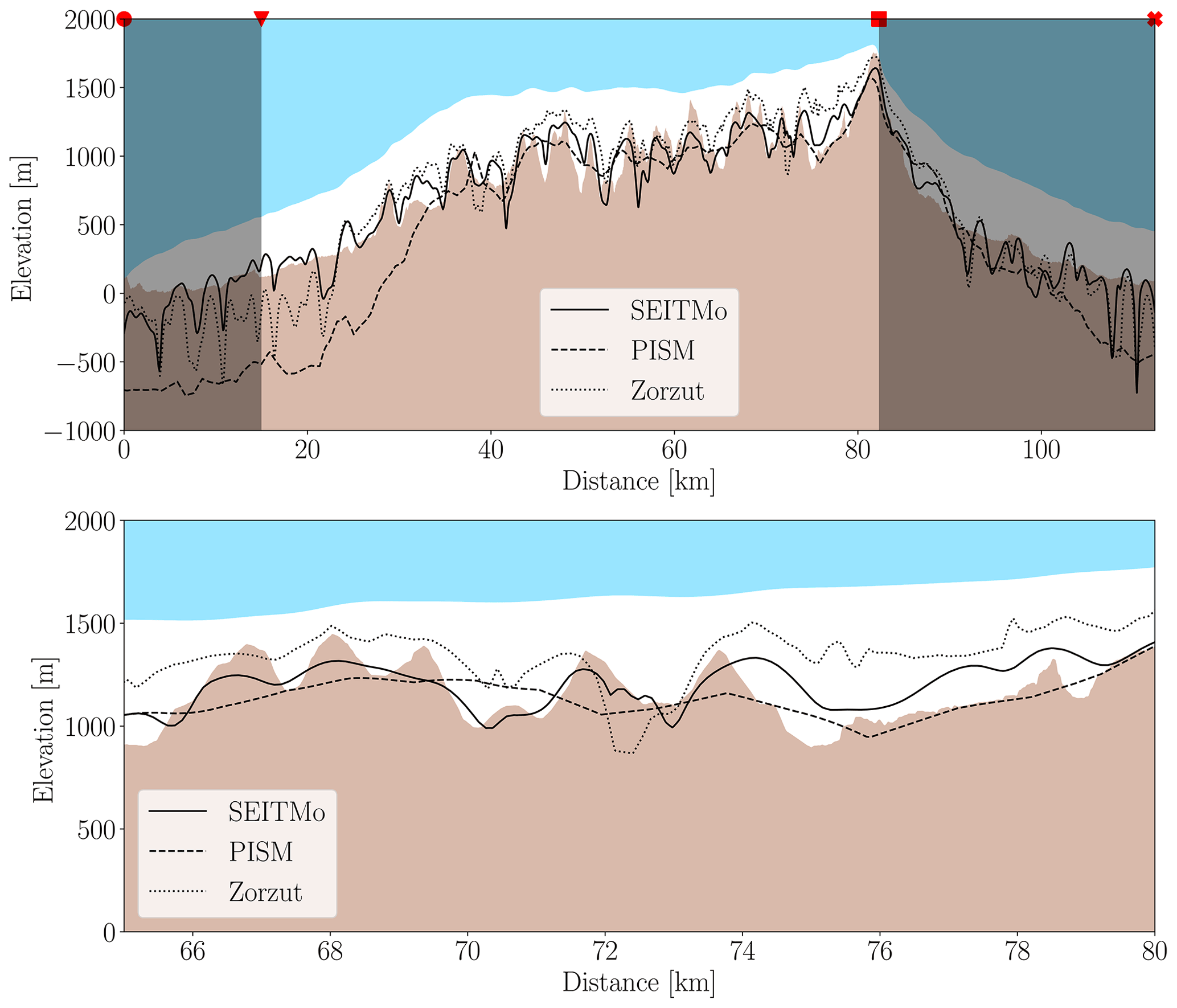
The OIB cross section with corresponding SEITMo, PISM, and Zorzut bedrock is shown in Fig. 2, where the surface elevation is from ArcticDEM (blue–white intersection) and the ice thickness in white is from OIB, resulting in the bedrock given by subtracting OIB from ArcticDEM in brown. The zoomed-in panel provides a visualisation of how well the different models perform in what could be an area of ice core drilling interest, i.e. thick ice, high elevation, and minimal horizontal ice flow. Figure 3 shows the modelled bedrock topographies (bottom) and ice thicknesses (top) of the entire ice cap.

Figure 3 SEITMo thickness (a) and bedrock topography (d). PISM ice thickness (b) and bedrock topography (e). Zorzut ice thickness (c) and bedrock topography (f). The black polygon in all panels marks the present-day ice cap margin as used in the SEITMo and Zorzut. The proposed drill site candidate (DSC) is marked in all panels. Coordinates are given in UTM zone 15N.

From Fig. 2 it can be seen that PISM overestimates the ice thickness at the outlet glaciers, though it captures the ice thickness over the central ice cap well. This overestimation is due to the fact that the bedrock is not adjusted below 500 m due to the relaxation parameter K. Hence, the model is not expected to do well in this area but only on the main ice cap. The middle panels of Fig. 3 show the PISM ice thickness (top) and corresponding bedrock topography (bottom) of the entire domain. The PISM ice cap covers a greater area than the present-day Müller Ice Cap, since no margin criteria have been used when running PISM.

After performing the minimisation problem of Zorzut, f_a is found to be 0.884, which is applied to the entire ice cap. Generally, it can be seen that Zorzut underestimates the ice thickness in the area between 74–80 km (zoomed-in part of Fig. 2), which is related to the relatively low ice velocities in the vicinity of the ice divide.

The RMSEs of the three models compared to the OIB thicknesses between 40–80 km in Fig. 2 are 136, 134, and 204 m for the SEITMo, PISM, and Zorzut, respectively. Likewise the mean absolute deviations (MADs) of the same part of the flight line are 112, 108, and 165 m for the SEITMo, PISM, and Zorzut, respectively. Thus, PISM and the SEITMo perform equally well in the area of interest, whereas Zorzut's significantly lower performance is most likely due to its constraints on the surface velocity.

A drill site candidate (DSC), which has to be further investigated with ground-penetrating radar, is proposed based on an ensemble of modelled ice thicknesses, surface melt, and surface velocities (Zinck, 2020c). The DSC location is shown in Fig. 3, and the corresponding SEITMo and PISM thicknesses are 579 and 535 m, respectively. The SEITMo thickness has been resampled onto the 900 m PISM grid before extracting the ice thickness to allow for a fairer comparison between the methods. It should be noted that the Zorzut thickness has not been included in the DSC selection. It is however noted that the 560 m thickness at the DSC estimated using the Zorzut approach falls between the PISM and SEITMo estimates.

5 Discussion

The SEITMo offers a fast estimate of ice thicknesses from sparse data. However, a stream-like pattern from the ice flux is clearly visible in the reconstructed ice thickness (Fig. 3a). Furthermore, sudden peaks in ice thickness also appear (Figs. 2 and 3), due to either low surface slope or ice flux as a result of the logarithm formulation in Eq. (6). One solution to these issues is to apply a smoothing to both the surface slope and the ice flux, as applying a smoothing to a single component will increase the extent of the issue of the other. Such fine-scale features are not trustworthy in simple models like the SEITMo, which is why the SEITMo result is interpolated onto a coarser grid before it is used in the DSC assessment, thereby reducing the impact of these features.

The key assumption in the SIA is that the ice deforms by simple bed-parallel shear. Such an approximation is reasonable on ice sheets where the horizontal extent is much greater than the vertical one. Whether this holds on the MIC is highly debatable. However, while the SIA is the justification for the functional form of Eq. (6), the model is eventually empirically tuned to reproduce thickness measurements. If sliding has a significant impact on ice flow, the regression will attempt to capture this effect by adjusting the free parameters (a, b, and k). For this reason we caution against a naive interpretation of the parameters in terms of, for example, a SIA flow law exponent (Eq. 5). Furthermore, it should be noted that the SEITMo is only expected to perform well when sufficient thickness measurements are present, which of course puts a constraint on the glaciers and ice caps it can be applied to.

Compared to the SEITMo, PISM is computationally heavier and relies on more input data. Focusing on the main ice cap in Fig. 2, PISM performs as well as the SEITMo. The outlet glaciers are of course not captured well due to the chosen relaxation parameter, which has no effect below 500 m. If the desire was to capture the entire domain well, one could keep the relaxation parameter as a constant and instead apply a tuning to the SMB. From the right panel of Fig. 1 there is an indication that HIRHAM5 in general overestimates the SMB. Further, it is a known issue that HIRHAM5 overestimates the precipitation in upsloping rough terrain (Schmidt et al., 2017), which might be the case over Axel Heiberg Island. It should be noted that Axel Heiberg Island is on the very edge of the HIRHAM5 domain (Mottram et al., 2017), which might have an influence on the SMB. However, the computational cost of the iterative PISM inversion severely limits the size of the model parameter space that is practical to search. Introducing additional parameters – e.g. to scale and offset SMB – would increase the dimensions of the parameter space hypercube. This was not feasible in the time allotted for this project. This is considered to be a major drawback of the iterative PISM approach and underscores the advantage of the SEITMo's insensitivity to SMB.

Zorzut is as fast as the SEITMo but has the lowest performance of all three models for reproducing the OIB thicknesses. Of special interest is the area between 74–80 km (Fig. 2), where Zorzut highly underestimates the ice thickness. This is because of the low velocities in the vicinity of the ice divide and the nature of the SIA, which is not valid at ice divides. The remotely sensed velocity estimates have a poor signal-to-noise ratio when ice velocities are small. Therefore, it is expected that the Zorzut approach has a lower performance near the ice divide (see Fig. 2). This also makes the model considerably less suited to the search for a possible drill site candidate where minimal horizontal flow is desired. Furthermore, the uncertainty in surface velocity products often exceeds the actual magnitude of the velocity in these slow-flowing areas. For comparison the ice thickness from Millan et al. (2022) was also inspected with respect to the OIB flight line. The thickness was found to also be underestimated in the vicinity of the ice divide, though not to the same degree as for Zorzut.

The overall thickness and topography patterns are similar between all three models. The SEITMo and PISM have comparable RMSEs and MADs, whereas Zorzut has both a higher RMSE and a higher MAD. Even though the SEITMo and Zorzut are only tuned to the part of the OIB flight line in between the red triangle and square (see Figs. 1 and 2), they still perform well on the rest of the flight line. This suggests that both models are also valid outside of the OIB flight line. The good fits of the SEITMo, in combination with its low computational costs and limited data requirements, make it an excellent candidate for fast ice thickness estimates. This is especially the case in areas with limited knowledge about past and present SMB.

The drill site candidate suggested here should be taken with caution, and further in situ measurements of ice thickness, surface melt, and surface elevation are highly recommended. Nonetheless, the DSC is based on an ensemble of thickness estimates, making the site a strong candidate.

6 Conclusions

Three methods for estimating the ice thickness distribution of the Müller Ice Cap were presented: firstly, a simple semi-empirical ice thickness model (SEITMo) based on the SIA; secondly, an iterative inverse method using PISM as a forward model; and thirdly, a velocity-based inversion of the SIA (Zorzut). The general ice thickness pattern of the ice cap is similar to a large degree for all three models. However, Zorzut strongly underestimates the ice thickness on the top of the ice cap in the vicinity of the ice divide, which is unfortunate as this is also the key area of interest in terms of a possible drill site. Further, the SEITMo and PISM show equally good results when compared to thickness measurements from Operation IceBridge. We demonstrate that the methods also differ strongly in terms of computational demands and need for input data, making the SEITMo, which is light in both respects, more favourable. Finally, one of the main advantages of the SEITMo, besides the computational efficiency, is the limited data the model relies on. This contrasts with the number of data that PISM relies on. It also entails that the SEITMo method could potentially be applied for global glacier thickness estimates, especially since it performs well on ice caps, which flowline methods often used in such estimates struggle with. This implies that one would have to do regional calibrations of the three tuning parameters for glaciers and ice caps with no ice thickness data available, since the SEITMo is only expected to perform well when sufficient thickness measurements are present.