An empirical algorithm to map perennial firn aquifers and ice slabs within the Greenland Ice Sheet using satellite L-band microwave radiometry

Perennial firn aquifers are subsurface meltwater reservoirs consisting of a meters-thick water-saturated firn layer that can form on spatial scales as large as tens of kilometers. They have been observed within the percolation facies of glaciated regions experiencing intense seasonal surface melting and high snow accumulation. Widespread perennial firn aquifers have been identified within the Greenland Ice Sheet (GrIS) via field expeditions, airborne ice-penetrating radar surveys, and satellite microwave sensors. In contrast, ice slabs are nearly continuous ice layers that can also form on spatial scales as large as tens of kilometers as a result of surface and subsurface water-saturated snow and firn layers sequentially refreezing following multiple melting seasons. They have been observed within the percolation facies of glaciated regions experiencing intense seasonal surface melting but in areas where snow accumulation is at least 25 % lower as compared to perennial firn aquifer areas. Widespread ice slabs have recently been identified within the GrIS via field expeditions and airborne ice-penetrating radar surveys, specifically in areas where perennial firn aquifers typically do not form. However, ice slabs have yet to be identified from space. Together, these two ice sheet features represent distinct, but related, sub-facies within the broader percolation facies of the GrIS that can be defined primarily by differences in snow accumulation, which influences the englacial hydrology and thermal characteristics of firn layers at depth.

Here, for the first time, we use enhanced-resolution vertically polarized L-band brightness temperature ($T_{\mathrm{V}}^{\mathrm{B}}$) imagery (2015–2019) generated using observations collected over the GrIS by NASA's Soil Moisture Active Passive (SMAP) satellite to map perennial firn aquifer and ice slab areas together as a continuous englacial hydrological system. We use an empirical algorithm previously developed to map the extent of Greenland's perennial firn aquifers via fitting exponentially decreasing temporal L-band signatures to a set of sigmoidal curves. This algorithm is recalibrated to also map the extent of ice slab areas using airborne ice-penetrating radar surveys collected by NASA's Operation IceBridge (OIB) campaigns (2010–2017). Our SMAP-derived maps show that between 2015 and 2019, perennial firn aquifer areas extended over 64 000 km², and ice slab areas extended over 76 000 km². Combined together, these sub-facies are the equivalent of 24 % of the percolation facies of the GrIS. As Greenland's climate continues to warm, seasonal surface melting will increase in extent, intensity, and duration. Quantifying the possible rapid expansion of these sub-facies using satellite L-band microwave radiometry has significant implications for understanding ice-sheet-wide variability in englacial hydrology that may drive meltwater-induced hydrofracturing and accelerated ice flow as well as high-elevation meltwater runoff that can impact the mass balance and stability of the GrIS.

1 Introduction

The recent launches of several satellite L-band microwave radiometry missions by NASA (Aquarius mission, Le Vine et al., 2007; Soil Moisture Active Passive (SMAP) mission, Entekhabi et al., 2010) and ESA (Soil Moisture and Ocean Salinity (SMOS), Kerr et al., 2001) have provided a new Earth-observation tool capable of detecting meltwater stored tens of meters to kilometers beneath the ice sheet surface. Jezek et al. (2015) recently demonstrated that in the high-elevation (3500 m a.s.l.) dry snow facies of the Antarctic Ice Sheet, meltwater stored in subglacial Lake Vostok can be detected as deep as 4 km beneath the ice sheet surface. Subglacial lakes represent radiometrically cold subsurface meltwater reservoirs. Upwelling L-band emission from the radiometrically warm bedrock underlying the subglacial lakes is effectively blocked by high reflectivity and attenuation at the interface between the bedrock and the overlying lake bottom. This results in a lower observed microwave brightness temperature (T^B) at the ice sheet surface as compared to other dry snow facies areas where bedrock contributes to L-band emission depth-integrated over the entire ice sheet thickness.

Similar to subglacial lakes, perennial firn aquifers also represent radiometrically cold subsurface meltwater reservoirs (Miller et al., 2020) consisting of a 4–25 m thick water-saturated firn layer (Koenig et al., 2014; Montgomery et al., 2017; Chu et al., 2018) that can form on spatial scales as large as tens of kilometers (Forster et al., 2014). Perennial firn aquifers have been identified via field expeditions (Forster et al., 2014), airborne ice-penetrating radar surveys (Miège et al., 2016), and satellite microwave sensors (Brangers et al., 2020; Miller et al., 2020) in the lower-elevation (<2000 m a.s.l.) percolation facies of the Greenland Ice Sheet (GrIS) at depths from between 1 and 40 m beneath the ice sheet surface. They exist in areas that experience intense seasonal surface melting and rain (>650 $\mathrm{mm}\mathrm{w}.\mathrm{e}.{\mathrm{yr}}^{-\mathrm{1}}$) during the melting season and high snow accumulation (>800 $\mathrm{mm}\mathrm{w}.\mathrm{e}.{\mathrm{yr}}^{-\mathrm{1}}$) during the freezing season (Forster et al., 2014). High snow accumulation in perennial firn aquifer areas thermally insulates water-saturated firn layers from the cold atmosphere, allowing seasonal meltwater to be stored in liquid form year-round if the overlying seasonal snow layer is sufficiently thick (Kuipers Munneke et al., 2014). Koenig et al. (2014) estimated that the volumetric fraction of meltwater stored within the pore space of Greenland's perennial firn aquifers just prior to melt onset ranges from between 10 % and 25 %, which limits the upward propagation of electromagnetic energy from greater depths within the ice sheet. Large volumetric fractions of meltwater within the firn pore space result in high reflectivity and attenuation at the interface between water-saturated firn layers and the overlying refrozen firn layers as well as between glacial ice or an impermeable layer and the overlying water-saturated firn layers. Upwelling L-band emission from deeper glacial ice and the underlying bedrock is effectively blocked.

While perennial firn aquifers are radiometrically cold, the slow refreezing of deeper firn layers saturated with large volumetric fractions of meltwater represents a significant source of latent heat that is continuously released throughout the freezing season. Refreezing of seasonal meltwater by the descending winter cold wave (Pfeffer et al., 1991), and the subsequent formation of embedded ice structures (i.e., horizontally oriented ice layers and ice lenses as well as vertically oriented ice pipes; Benson et al., 1960; Humphrey et al., 2012; Harper et al., 2012) within the upper snow and firn layers, represents a secondary source of latent heat. These heat sources help maintain meltwater at depth. Perennial firn aquifer areas are radiometrically warmer than other percolation facies areas where the single source of latent heat is via refreezing of seasonal meltwater. This results in a higher observed T^B at the ice sheet surface during the freezing season as compared to other percolation facies areas where seasonal meltwater is fully refrozen and stored exclusively as embedded ice.

Recently, mapping the extent of Greenland's perennial firn aquifers from space was demonstrated using satellite L-band microwave radiometry (Miller et al., 2020). Exponentially decreasing temporal L-band signatures observed in enhanced-resolution vertically polarized L-band brightness temperature ($T_{\mathrm{V}}^{\mathrm{B}}$) imagery (2015–2016) generated using observations collected over the GrIS by the microwave radiometer on NASA's SMAP satellite (Long et al., 2019) were correlated with a single year of perennial firn aquifer detections (Miège et al., 2016). These detections were identified via the Center for Remote Sensing of Ice Sheets (CReSIS) Multi-Channel Coherent Radar Depth Sounder (MCoRDS) flown by NASA's Operation IceBridge (OIB) campaigns (Rodriguez-Morales et al., 2014). An empirical algorithm to map extent was developed by fitting temporal L-band signatures to a set of sigmoidal curves derived from the continuous logistic model.

The relationship between the radiometric, and thus the physical, temperature of perennial firn aquifer areas, as compared to other percolation facies areas, forms the basis of the empirical algorithm. Miller et al. (2020) hypothesized that the dominant control on the relatively slow exponential rate of T^B decrease over perennial firn aquifer areas is physical temperature versus depth. L-band emission from the radiometrically warm upper snow and firn layers decreases during the freezing season as embedded ice structures slowly refreeze at increased depths below the ice sheet surface. In the percolation facies, refreezing of seasonal meltwater results in the formation of an intricate network of embedded ice structures that are large (10–100 cm long, 10–20 cm wide; Jezek et al., 1994) relative to the L-band wavelength (21 cm). Embedded ice structures induce strong volume scattering (Rignot et al., 1993; Rignot, 1995) that decreases T^B (Zwally, 1977; Swift et al., 1985; Jezek et al., 2018).

Ice slabs are 1–16 m thick nearly continuous ice layers that can form on spatial scales as large as tens of kilometers as a result of surface and subsurface water-saturated snow and firn layers sequentially refreezing following multiple melting seasons (Machguth et al., 2016; MacFerrin et al., 2019). Over time, they become dense low-permeability solid-ice layers overlying deeper permeable firn layers. Ice slabs have been identified via field expeditions and airborne ice-penetrating radar surveys in the lower-elevation (<2000 m a.s.l.) percolation facies of the GrIS at depths from between 1 and 20 m beneath the ice sheet surface (MacFerrin et al., 2019). They exist in areas that experience intense seasonal surface melting and rain (excess melt of 266–573 $\mathrm{mm}\mathrm{w}.\mathrm{e}.{\mathrm{yr}}^{-\mathrm{1}}$; see MacFerrin et al., 2019, for a description) during the melting season and lower snow accumulation ($<\mathrm{572}\pm \mathrm{32}$ $\mathrm{mm}\mathrm{w}.\mathrm{e}.{\mathrm{yr}}^{-\mathrm{1}}$) during the freezing season as compared to perennial firn aquifer areas (MacFerrin et al., 2019). Lower snow accumulation in ice slab areas results in a seasonal snow layer that is insufficiently thick to thermally insulate water-saturated firn layers and seasonal meltwater is instead stored as embedded ice.

Refreezing of seasonal meltwater by the descending winter cold wave, and the subsequent formation of ice slabs as well as other embedded ice structures within the upper snow and firn layers, is the single source of latent heat. While ice slab areas are radiometrically warmer than other percolation facies areas with a lower volumetric fraction of embedded ice, they are radiometrically colder than perennial firn aquifer areas. This results in typically higher observed T^B at the ice sheet surface during the freezing season in ice slab areas, as compared to other percolation facies areas, but typically lower observed T^B as compared to perennial firn aquifer areas. Similar to temporal L-band signatures over perennial firn aquifer areas, temporal L-band signatures over ice slab areas are exponentially decreasing during the freezing season; however, the rate of T^B decrease is slightly more rapid.

In this study, we exploit the observed sensitivity of L-band emission to variability in the depth- and time-integrated dielectric and geophysical properties of the percolation facies of the GrIS to map perennial firn aquifer and ice slab areas together as a continuous englacial hydrological system using satellite L-band microwave radiometry.

2 Methods

We adapt our previously developed empirical algorithm to map the extent of Greenland's perennial firn aquifers (Miller et al., 2020) using a multi-year calibration technique. We use enhanced-resolution L-band $T_{\mathrm{V}}^{\mathrm{B}}$ imagery (2015–2019) generated using observations collected over the GrIS by the microwave radiometer on NASA's SMAP satellite (Long et al., 2019) and airborne ice-penetrating radar surveys collected by NASA's OIB campaigns (Rodriguez-Morales et al., 2014). First, we correlate (1) a “firn saturation” parameter derived from a simple two-layer L-band brightness temperature model; (2) maximum and (3) minimum $T_{\mathrm{V}}^{\mathrm{B}}$ values; and (4) exponentially decreasing temporal L-band signatures, with 5 years of perennial firn aquifer detections (2010–2014) identified via the CReSIS Accumulation Radar (AR) (Miège et al., 2016) and 3 years of additional detections (2015–2017) more recently identified via MCoRDS (Miller et al., 2020). Next, we extend our empirical algorithm to map the extent of ice slab areas. We correlate the SMAP-derived parameters with 5 years of ice slab detections (2010–2014) recently identified via AR (MacFerrin et al., 2019). Finally, we recalibrate our empirical model to map the extent of perennial firn aquifer and ice slab areas over the percolation facies. Interannual variability in extent is not resolved in this study; however, it will be explored further in future work.

2.1 SMAP enhanced-resolution L-band T^B imagery

The key science objectives of NASA's SMAP mission (https://smap.jpl.nasa.gov/, last access: 4 January 2022) are to map terrestrial soil moisture and freeze/thaw state over Earth's land surfaces from space. However, the global L-band T^B observations collected by the SMAP satellite also have cryospheric applications. Mapping perennial firn aquifer and ice slab areas over Earth's polar ice sheets represents an interesting analog and an innovative extension of the SMAP mission's science objectives. The SMAP satellite was launched on 31 January 2015 and carries a microwave radiometer that operates at an L-band frequency of 1.41 GHz (Enkentabi et al., 2010). It is currently collecting observations of vertically and horizontally polarized T^B over Greenland. The surface incidence angle is 40^∘, and the radiometric accuracy is approximately 1.3 K (Piepmeier et al., 2017).

The Scatterometer Image Reconstruction (SIR) algorithm was originally developed to reconstruct coarse-resolution satellite radar scatterometry imagery on a higher-spatial-resolution grid (Long et al., 1993; Early and Long, 2001). The SIR algorithm has been adapted for coarse-resolution satellite microwave radiometry imagery (Long and Daum, 1998; Long and Brodzik, 2016; Long et al., 2019). The microwave radiometer form of the SIR algorithm (rSIR) uses the measurement response function (MRF) for each observation, which is a smeared version of the antenna pattern. Using the overlapping MRFs, the rSIR algorithm reconstructs T^B from the spatially filtered low-resolution sampling provided by the observations. In effect, it generates an MRF-deconvolved T^B image. Combining multiple orbital passes increases the sampling density, which improves both the accuracy and resolution of the SMAP enhanced-resolution T^B imagery (Long et al., 2019).

Over Greenland, the rSIR algorithm combines satellite orbital passes that occur between 08:00 and 16:00 local time of day to reconstruct SMAP enhanced-resolution T^B imagery twice-daily (i.e., morning and evening orbital pass interval, respectively). T^B imagery is projected on a Northern Hemisphere (NH) Equal-Area Scalable Earth Grid (EASE-Grid 2.0; Brodzik et al., 2012) at a 3.125 km rSIR grid cell spacing (e.g., Fig. 1). The effective resolution for each grid cell is dependent on the number of observations used in the rSIR reconstruction and is coarser than the rSIR grid cell spacing. While the effective resolution of conventionally processed SMAP T^B imagery posted on a 25 km grid is approximately 30 km (e.g., Fig. 1a), the effective resolution of SMAP enhanced-resolution T^B imagery posted on a 3.125 km grid is approximately 18 km (e.g., Fig. 1b), an improvement of 60 % (Long et al., 2019).

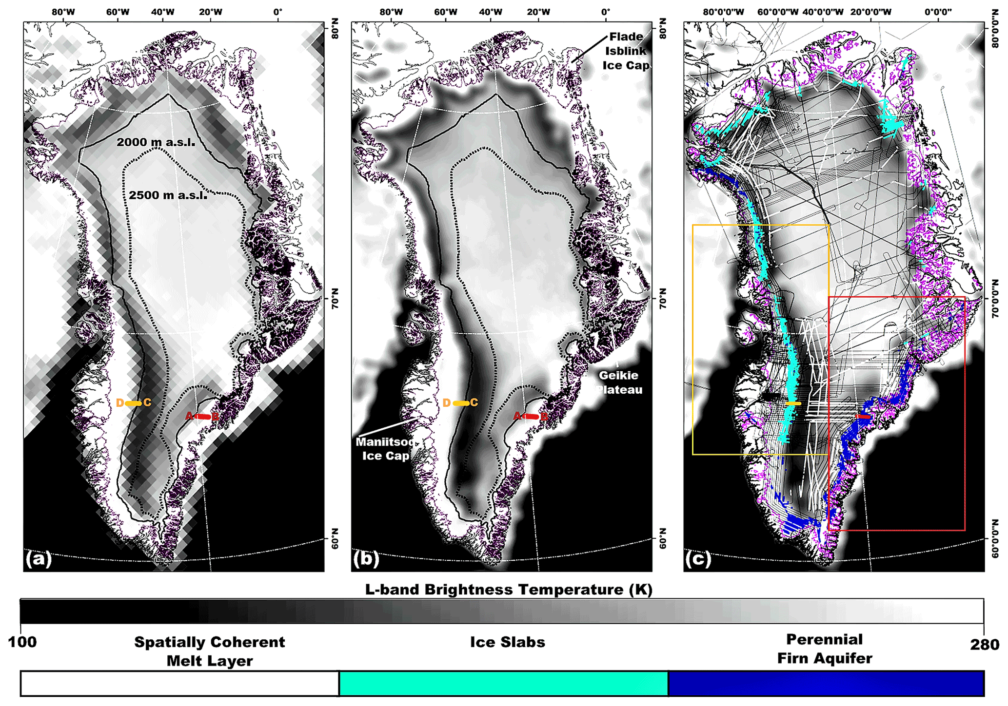
Figure 1 (a) Gridded (25 km gridding, 30 km effective resolution) and (b) enhanced-resolution (3.125 km gridding, 18 km effective resolution) L-band $T_{\mathrm{V}}^{\mathrm{B}}$ imagery generated using observations collected on 15 April 2016 by the microwave radiometer on the SMAP satellite during the evening orbital pass interval over Greenland (Long et al., 2019) overlaid with the 2000 m a.s.l. contour (black line) and the 2500 m a.s.l. contour (dotted black line; Howat et al., 2014), the ice sheet extent (purple line; Howat et al., 2014), and the coastline (black peripheral line; Wessel and Smith, 1996). (c) SMAP enhanced-resolution L-band $T_{\mathrm{V}}^{\mathrm{B}}$ imagery overlaid with AR- and MCoRDS-derived 2010–2017 perennial firn aquifer (blue shading; Miège et al., 2016), 2010–2014 ice slab (cyan shading; MacFerrin et al., 2019), and 2012 spatially coherent melt layer (white shading; Culberg et al., 2021) detections along OIB flight lines (black interior lines); zoom areas over southeastern Greenland (red box; Fig. 2a) and southwestern Greenland (orange box; Fig. 2b); and AR radargram transect A-B (red line; Fig. 3a) and C-D (orange line; Fig. 3b).

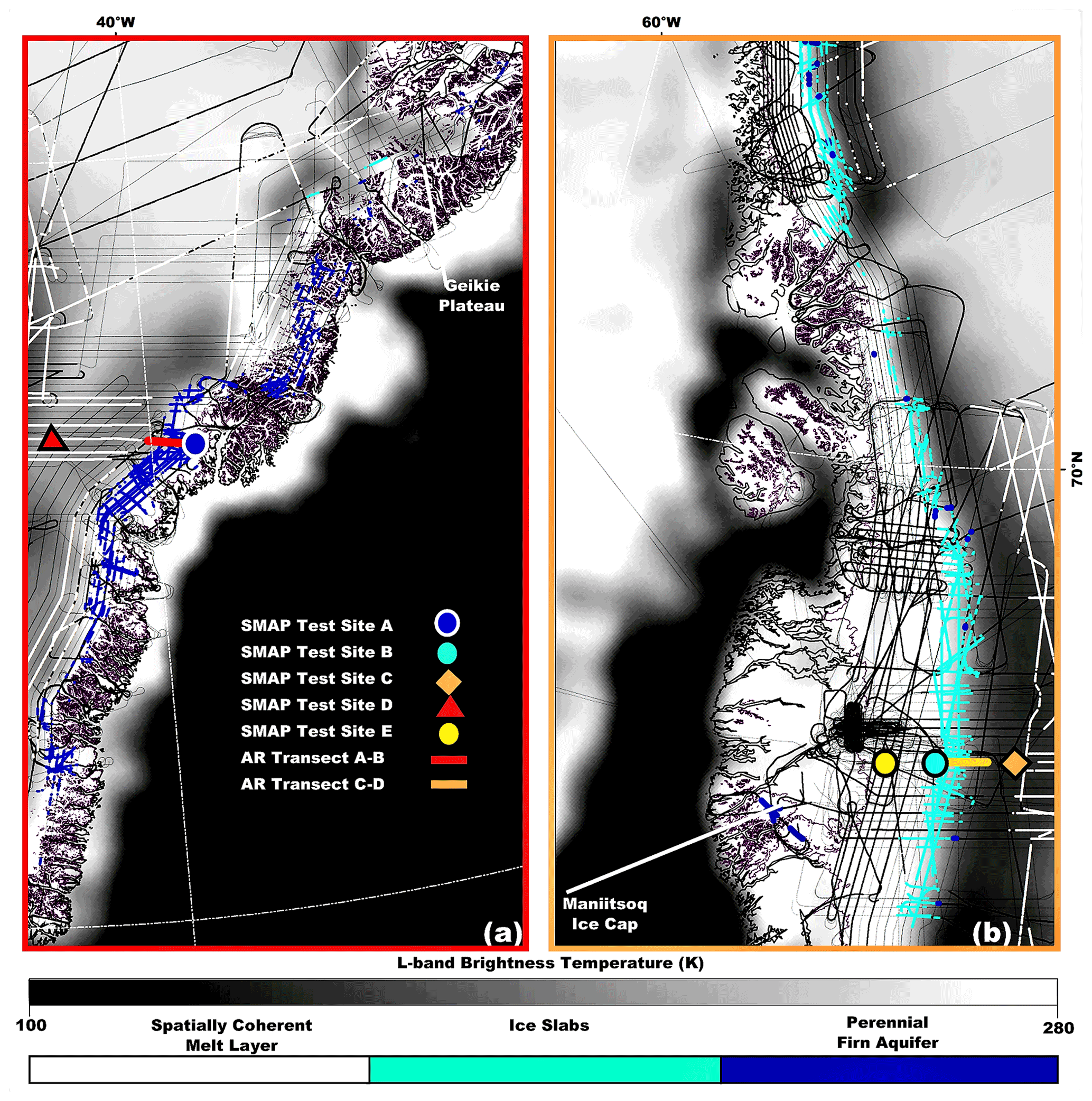
Figure 2 Enhanced-resolution (3.125 km gridding, 30 km effective resolution) L-band $T_{\mathrm{V}}^{\mathrm{B}}$ imagery generated using observations collected on 15 April 2016 by the microwave radiometer on the SMAP satellite during the evening orbital pass interval over (a) southeastern Greenland (red box; Fig. 1c) and (b) southwestern Greenland (orange box; Fig. 1c,) (Long et al., 2019) overlaid with the ice sheet extent (purple line; Howat et al., 2014); the coastline (black peripheral line; Wessel and Smith, 1996); the AR- and MCoRDS-derived 2010–2017 perennial firn aquifer (blue shading; Miège et al., 2016), 2010–2014 ice slab (cyan shading; MacFerrin et al., 2019), and 2012 spatially coherent melt layer (white shading; Culberg et al., 2021) detections along OIB flight lines (black interior lines); AR radargram transect A-B (red line; Fig. 3a) and C-D (orange line; Fig. 3b); and SMAP Test Site A (blue circle; Fig. 4a), B (cyan circle; Fig. 4b), C (orange diamond; Fig. 4c), D (red triangle; Fig. 4d), and E (yellow circle; Fig. 4e).

As previously noted, for our analysis of the percolation facies we use SMAP enhanced-resolution $T_{\mathrm{V}}^{\mathrm{B}}$ imagery over the GrIS. Compared to the horizontally polarized channel, the vertically polarized channel exhibits decreased sensitivity to variability in the volumetric fraction of meltwater, which is attributed to reflection coefficient differences between channels (Miller et al., 2020). Using the vertically polarized channel also results in a reduced chi-squared error statistic when fitting $T_{\mathrm{V}}^{\mathrm{B}}$ time series to the sigmoid function (Sect. 2.3.4). We construct $T_{\mathrm{V}}^{\mathrm{B}}$ imagery that alternates morning and evening orbital pass observations annually, beginning and ending just prior to melt onset. The Greenland Ice Mapping Project (GIMP) Land Ice and Ocean Classification Mask and Digital Elevation Model (Howat et al., 2014) are projected on the NH EASE-Grid 2.0 at a 3.125 km rSIR grid cell spacing. The derived ice mask includes the Greenland Ice Sheet and the peripheral ice caps, including Maniitsoq and Flade Isblink. $T_{\mathrm{V}}^{\mathrm{B}}$ imagery between 1 April 2015 and 31 March 2019 is ice-masked, and an elevation for each rSIR grid cell is calculated.

2.2 Airborne ice-penetrating radar surveys

AR and MCoRDS (Rodriguez-Morales et al., 2014) were flown over the GrIS on a P-3 aircraft in April and May between 2010 and 2017. The AR instrument operates at a center frequency of 750 MHz with a bandwidth of 300 MHz, resulting in a range resolution in firn of 0.53 m (Lewis et al., 2015). The collected data have an along-track resolution of approximately 30 m with 15 m spacing between traces in the final processed radargrams. At a nominal flight altitude of 500 m above the ice sheet surface, the cross-track resolution varies between 20 m for a smooth surface and 54 m for a rough surface with no appreciable layover. The MCoRDS instrument operated at three different frequency configurations: (1) a center frequency of 195 MHz with a bandwidth of 30 MHz (2010–2014, 2017), (2) a center frequency of 315 MHz with a bandwidth of 270 MHz (2015), and (3) a center frequency of 300 MHz with a bandwidth of 300 MHz (2016). The vertical range resolution in firn for each of these frequency configurations is 5.3, 0.59, and 0.53 m, respectively (CReSIS, 2016). The collected data have an along-track resolution of approximately 25 m with 14 m spacing between traces in the final processed radargrams. At the same nominal flight altitude of 500 m, the cross-track resolution varies between 40 m for a smooth surface in the highest bandwidth configuration and 175 m for a rough surface with no appreciable layover in the lowest bandwidth configuration.

The multi-year calibration technique uses perennial firn aquifer detections previously identified along OIB flight lines via AR (2010–2014) and MCoRDS (2015–2017) radargram profiles and the methodology described in Miège et al. (2016). Bright lower reflectors that undulate with the local topographic gradient underneath which reflectors are absent in the percolation facies are interpreted as the upper surface of meltwater stored within perennial firn aquifers (e.g., Fig. 3a). The large dielectric contrast between refrozen and water-saturated firn layers results in high reflectivity at the interface. However, the presence of meltwater increases attenuation, limiting the downward propagation of electromagnetic energy through the water-saturated firn layer. The total number of AR derived perennial firn aquifer detections is 325 000, corresponding to a total extent of 98 km². The analysis assumes a smooth surface, which is typical of much of the percolation facies, and a grid cell size of 15 m×20 m. The total number of MCoRDS-derived perennial firn aquifer detections is 142 000, corresponding to a total extent of 80 km². This analysis also assumes a smooth surface and a grid cell size of 14 m×40 m. The combined total number of grid cells (467 000) and total extent (178 km²) is significantly larger than the total number of MCoRDS-derived grid cells (78 000) and total extent (44 km²) calculated for 2016 (Miller et al., 2020). Perennial firn aquifer detections are mapped in northwestern, southern, and south and central eastern Greenland as well as the Maniitsoq and Flade Isblink ice caps (Figs. 1c and 2a).

We project AR- and MCoRDS-derived perennial firn aquifer detections on the NH EASE-Grid 2.0 at an rSIR grid cell spacing of 3.125 km. Each rSIR grid cell has an extent of approximately 10 km². The total number of rSIR grid cells with at least one perennial firn aquifer detection is 800, corresponding to a total extent of 8000 km². However, given the limited AR and MCoRDS grid cell coverage, less than 1 % of the rSIR grid cell extent has airborne ice-penetrating radar survey coverage. As compared to the total number of MCoRDS-derived perennial firn aquifer detections (780) calculated for 2016 (Miller et al., 2020), the total number of rSIR grid cells with at least one detection is only increased by 20 for the multi-year calibration technique, corresponding to an increased total extent of 200 km².

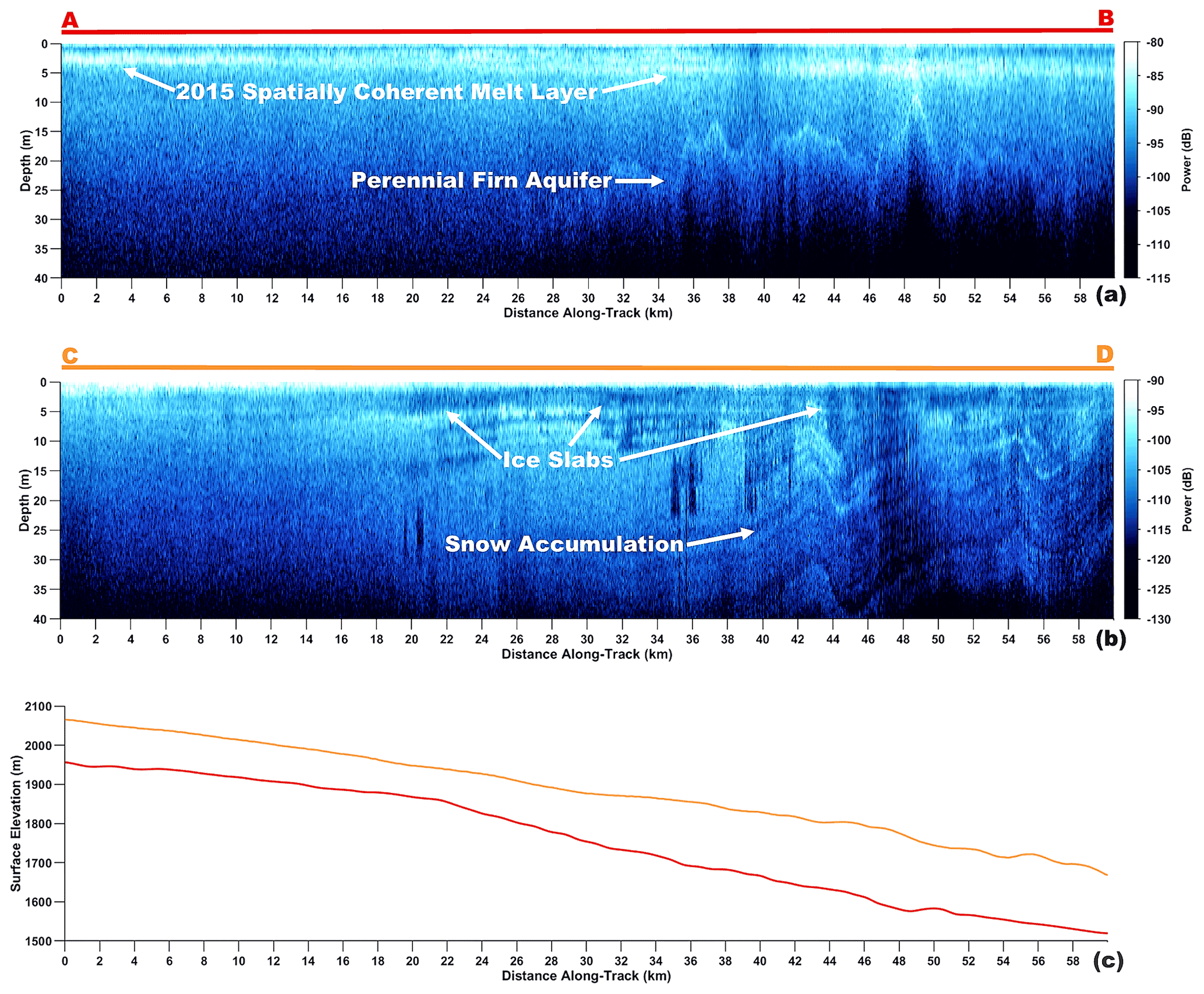
Figure 3 AR radargram transect (a) A-B (red line; Fig. 2a) collected on 22 April 2017 and (b) C-D (orange line; Fig. 2b) collected on 5 May 2017 (Rodriguez-Morales et al., 2014). (c) AR radargram transect A-B (red line) and C-D (orange line) elevation profiles. The exceptionally bright upper surface-parallel reflector in panel (a) is a spatially coherent melt layer. The bright lower reflector in panel (a) is the upper surface of meltwater stored within a perennial firn aquifer. The thick dark surface-parallel regions of low reflectivity in panel (b) are ice slabs. The alternating sequences of bright and dark surface-parallel reflectors in panel (b) are seasonal snow accumulation layers.

We also use ice slab detections previously identified along OIB flight lines via AR (2010–2014) radargram profiles and the methodology described in MacFerrin et al. (2019) in the multi-year calibration technique. Thick dark surface-parallel regions of low reflectivity in the percolation facies are interpreted as ice slabs (e.g., Fig. 3b). The large dielectric contrast between ice slabs and the overlying and underlying snow and firn layers results in high reflectivity at the interfaces. However, electromagnetic energy is not scattered or absorbed within the homogeneous ice slab; it instead propagates downward through the layer and into the deeper firn layers. The total number of AR-derived ice slab detections is 505 000, corresponding to a total extent of 283 km². Ice slab detections are mapped in western, central and northeastern, and northern Greenland as well as the Flade Isblink Ice Cap (Figs. 1c and 2b).

We project the AR-derived ice slab detections on the NH EASE-Grid 2.0 at an rSIR grid cell spacing of 3.125 km. The total number of rSIR grid cells with at least one ice slab detection is 2000, corresponding to a total extent of 20 000 km². However, less than 2 % of the rSIR grid cell extent has airborne ice-penetrating radar survey coverage.

An advantage of the multi-year calibration technique as compared to the single-coincident year calibration technique (Miller et al., 2020) is that it increases the number of rSIR grid cells that can be assessed. It also provides repeat targets that can account for variability in the depth- and time-integrated dielectric and geophysical properties that influence the radiometric temperature in stable perennial firn aquifer and ice slab areas. Uncertainty is introduced by correlating the SMAP-derived parameters with AR- and MCoRDS-derived detections that are not coincident in time. The multi-year calibration technique assumes the extent of each area remains stable, which is not necessarily the case as climate extremes (Cullather et al., 2020) can influence each of these sub-facies. The assumption of stability neglects boundary transitions in the extent of perennial firn aquifer areas associated with refreezing of shallow water-saturated firn layers, englacial drainage of meltwater into crevasses at the periphery (Poinar et al., 2017, 2019), and transient upslope expansion (Montgomery et al., 2017). Once formed, ice slabs are essentially permanent features within the upper snow and firn layers of the percolation facies until they are compressed into glacial ice. However, they may transition into superimposed ice at the lower boundary of ice slab areas or rapidly expand upslope, particularly following extreme melting seasons (MacFerrin et al., 2019). Thus, we simply consider our mapped extent a high-probability area for the preferential formation of each of these sub-facies, with continued presence dependent on seasonal surface melting and snow accumulation in subsequent years.

Annual perennial firn aquifer and ice slab detections that may introduce significant uncertainty into the multi-year calibration technique include those following the 2010 melting season, which was exceptionally long (Tedesco et al., 2011); the anomalous 2012 melting season, during which seasonal surface melting extended across 99 % of the GrIS (Nghiem et al., 2012); and the 2015 melting season, which was especially intense in western and northern Greenland (Tedesco et al., 2016). Following these extreme melting seasons, significant changes in the dielectric and geophysical properties likely occurred across large portions of the GrIS, including perennial firn aquifer recharging resulting in increases in meltwater volume and decreases in the depth to the upper surface of stored meltwater. The upper snow and firn layers of the dry snow facies and percolation facies were also saturated with relatively large volumetric fractions of meltwater as compared to the negligible-to-limited volumetric fractions of meltwater that percolates during more typical seasonal surface melting over the GrIS.

Seasonal meltwater was refrozen into spatially coherent melt layers following the 2010 and 2012 melting seasons (Culberg et al., 2021) as well as more recently following the 2015 and 2018 melting seasons identified as part of the temporal L-band signature analysis in this study (Sect. 2.3.1). As compared to ice slabs, which are dense low-permeability solid-ice layers, spatially coherent melt layers are a network of embedded ice structures primarily consisting of discontinuous horizontally oriented ice layers and ice lenses sparsely connected via vertically oriented ice pipes (Culberg et al., 2021). Spatially coherent melt layers are relatively thin (0.2 cm–2 m) and can rapidly form across the high-elevation (up to 3200 m a.s.l.) dry snow facies at depths of less than 1 m beneath the ice sheet surface following a single extreme melting season. They can further merge together into thicker solid-ice layers following multiple extreme melting seasons. Spatially coherent melt layers are exceptionally bright in AR radargrams (e.g., Fig. 3a). The large dielectric contrast between the spatially coherent melt layer and the overlying, underlying, and interior snow and firn layers results in high reflectivity at the interfaces. However, electromagnetic energy still propagates downward through the high-reflectivity layer into the deeper firn layers. Culberg et al. (2021) recently demonstrated mapping the extent of spatially coherent melt layers formed following the 2012 melting season (Nghiem et al., 2012) via AR (Figs. 1c and 2).

2.3 Empirical algorithm

2.3.1 Temporal L-band signatures

T^B expresses the satellite-observed magnitude of thermal emission and is influenced by the microwave instrument's observation geometry as well as the depth- and time-integrated dielectric and geophysical properties of the ice sheet (Ulaby et al., 2014). The most significant geophysical property influencing T^B is the volumetric fraction of meltwater within the snow and firn pore space (Mätzler and Hüppi, 1989). During the melting season, the upper snow and firn layers of the percolation facies are saturated with large volumetric fractions of meltwater that percolates vertically into the deeper firn layers (Benson, 1960; Humphrey et al., 2012). Increases in the volumetric fraction of meltwater result in rapid relative increases in the imaginary part of the complex dielectric constant (Tiuiri et al., 1984). This typically increases T^B and decreases volume scattering and penetration depth. The L-band penetration depth can rapidly decrease from tens to hundreds of meters to less than a meter, dependent on the local snow and firn conditions. During the freezing season, surface and subsurface water-saturated snow and firn layers and embedded ice structures subsequently refreeze. Decreases in the volumetric fraction of meltwater result in rapid relative decreases in the imaginary part of the complex dielectric constant. This decreases T^B and increases volume scattering and penetration depth. The L-band penetration depth increases back to tens to hundreds of meters on variable timescales.

We analyze melting and freezing seasons in temporal L-band signatures exhibited in $T_{\mathrm{V}}^{\mathrm{B}}$ time series over and near the AR- and MCoRDS-derived perennial firn aquifer and ice slab detections projected on the NH EASE-Grid 2.0 (Fig. 4 and Table 1). We project ice surface temperature observations calculated using thermal infrared brightness temperature collected by the Moderate Resolution Imaging Spectroradiometer (MODIS) on the Terra and Aqua satellites (Hall et al., 2012) on the NH EASE-Grid 2.0 at a 3.125 km rSIR grid cell spacing. We then derive melt onset and surface freeze-up dates for each rSIR grid cell using the methodology described in Miller et al. (2020). We set a threshold of ice surface temperature $>-\mathrm{1}$ ^∘C for meltwater detection (Nghiem et al., 2012), consistent with the ±1 ^∘C accuracy of the ice surface temperature observations. For temperatures that are close to 0 ^∘C, ice surface temperatures are closely compatible with contemporaneous NOAA near-surface air temperature observations (Shuman et al., 2014). Melt onset and surface freeze-up dates are overlaid on $T_{\mathrm{V}}^{\mathrm{B}}$ time series to partition the melting and freezing seasons. Melt onset dates typically occur between April and July, and surface freeze-up dates typically occur between July and September. The melting season increases in duration moving downslope from the dry snow facies and ranges from a single day in the highest elevations (>2500 m) of the percolation facies to 150 d in the ablation facies. Similarly, the freezing season decreases in duration moving downslope and ranges between 215 and 365 d.

Figure 4 Temporal L-band signatures that alternate morning (white symbols) and evening (colored symbols) orbital pass interval enhanced-resolution $T_{\mathrm{V}}^{\mathrm{B}}$ generated using observations collected over the GrIS by the microwave radiometer on the SMAP satellite (Long et al., 2019) over (a) SMAP Test Site A (blue circles; Fig. 2a), (b) B (cyan circles; Fig. 2b), (c) C (orange diamonds; Fig. 2b), (d) D (red triangles; Fig. 2a), and (e) E (yellow circles; Fig. 2b). Melt onset (red lines) and surface freeze-up (blue lines) dates derived from thermal infrared T^B collected by MODIS on the Terra and Aqua satellites (Hall et al., 2012). AR radargram transect A-B (red dashed line; Fig. 3a) collected on 22 April 2017, and C-D (orange dashed line; Fig. 3b) collected on 5 May 2017.

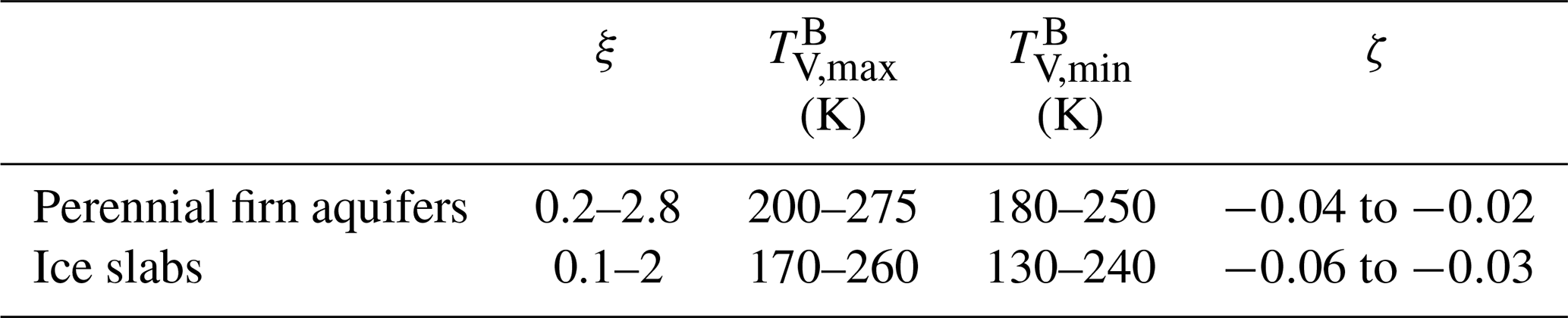
Table 1 MODIS-derived total number of days in the melting and freezing seasons; SMAP-derived maximum vertically polarized L-band brightness temperature ($T_{\text{V,max}}^{\mathrm{B}}$); minimum vertically polarized L-band brightness temperature ($T_{\text{V,min}}^{\mathrm{B}}$); timescales of exponential decrease following the surface freeze-up date for perennial firn aquifer, ice slab, percolation facies, dry snow facies, and wet snow facies areas.

Over perennial firn aquifer areas (e.g., Fig. 4a, SMAP Test Site A: 66.2115^∘ N, 39.1795^∘ W; 1625 m a.s.l.), maximum $T_{\mathrm{V}}^{\mathrm{B}}$ ($T_{\text{V,max}}^{\mathrm{B}}$) values are radiometrically warm during the melting season. Vertically percolating meltwater and gravity-driven meltwater drainage seasonally recharges perennial firn aquifers at depth (Fountain and Walder, 1998). Minimum $T_{\mathrm{V}}^{\mathrm{B}}$ ($T_{\text{V,min}}^{\mathrm{B}}$) values remain radiometrically warm during the freezing season as a result of latent heat continuously released by the slow refreezing of the deeper firn layers that are saturated with large volumetric fractions of meltwater (Miller et al., 2020). Temporal L-band signatures exhibit slow exponential decreases and approach, and sometimes achieve, stable $T_{\mathrm{V}}^{\mathrm{B}}$ values. $T_{\mathrm{V}}^{\mathrm{B}}$ can decrease by more than 50 K during the freezing season, which represents the descent of the upper surface of stored meltwater by depths of meters to tens of meters beneath the ice sheet surface (Miège et al., 2016).

Over ice slab areas (e.g., Fig. 4b, SMAP Test Site B: 66.8850^∘ N, 42.7765^∘ W; 1817 m a.s.l.), $T_{\text{V,max}}^{\mathrm{B}}$ values are typically radiometrically colder than over perennial firn aquifer areas during the melting season. The presence of dense low-permeability solid-ice layers reduces the snow and firn pore space available to store seasonal meltwater at depth. Meltwater may alternatively run off ice slabs downslope towards the wet snow facies. $T_{\text{V,min}}^{\mathrm{B}}$ values are also typically radiometrically colder than over perennial firn aquifer areas during the freezing season as a result of the absence of meltwater stored at depth. Temporal L-band signatures exhibit exponential decreases that are slightly more rapid than over perennial firn aquifer areas and often achieve stable $T_{\mathrm{V}}^{\mathrm{B}}$ values.

Over other percolation facies areas (e.g., Fig. 4c, SMAP Test Site C: 66.9024^∘ N, 44.7528^∘ W; 2350 m a.s.l.), where seasonal meltwater is fully refrozen and stored exclusively as embedded ice, $T_{\text{V,max}}^{\mathrm{B}}$ values are typically radiometrically colder than over perennial firn aquifer and ice slab areas during the melting season. $T_{\text{V,min}}^{\mathrm{B}}$ values are also typically radiometrically cold during the freezing season. Temporal L-band signatures exhibit rapid exponential decreases and achieve stable $T_{\mathrm{V}}^{\mathrm{B}}$ values. However, over the highest elevations (>2500 m a.s.l.) of the percolation facies approaching the dry snow line, where seasonal surface melting and the formation of embedded ice structures is limited, $T_{\text{V,min}}^{\mathrm{B}}$ values remain radiometrically warm during the freezing season. $T_{\mathrm{V}}^{\mathrm{B}}$ decreases, often step responses exceeding 10 K, are a result of an increase in volume scattering from newly formed embedded ice structures within a spatially coherent melt layer. Temporal L-band signatures that increase several K on timescales of years indicate the burial of spatially coherent melt layers formed following the 2010, 2012, 2015, and 2018 melting seasons by snow accumulation.

Exponentially decreasing temporal L-band signatures transition smoothly between perennial firn aquifer, ice slab, and other percolation facies areas – there are no distinct temporal L-band signatures that delineate boundaries between these sub-facies. Boundary transitions between the dry snow facies and wet snow facies, however, are delineated above and below the percolation facies. Over the dry snow facies (e.g., Fig. 4d, SMAP Test Site D: 66.3649^∘ N, 43.2115^∘ W; 2497 m a.s.l.), $T_{\text{V,max}}^{\mathrm{B}}$ and $T_{\text{V,min}}^{\mathrm{B}}$ values are radiometrically warm during the melting and freezing seasons. Temporal L-band signatures that increase on timescales of years are observed throughout the dry snow facies at elevations as high as Summit Station (3200 m a.s.l.) and indicate the burial of the spatially coherent melt layer formed following the 2012 melting season (Nghiem et al., 2012) by snow accumulation (Culberg et al., 2021). Over the wet snow facies (e.g., Fig. 4e, SMAP Test Site E: 67.3454^∘ N, 48.4789^∘ W; 1469 m a.s.l.), where seasonal meltwater is fully refrozen and stored as superimposed ice$,T_{\text{V,max}}^{\mathrm{B}}$ values are radiometrically warm during the melting season. As compared to the percolation facies, where temporal L-band signatures exhibit rapid increases following melt onset, temporal L-band signatures reverse and exhibit rapid decreases. These reversals are a result of high reflectivity and attenuation at the fully water saturated snow layer and/or at the wet rough superimposed ice–air interface. Meltwater runs off superimposed ice downslope towards the ablation facies. $T_{\text{V,min}}^{\mathrm{B}}$ values remain radiometrically warm during the freezing season. Temporal L-band signatures exhibit rapid increases and achieve stable $T_{\mathrm{V}}^{\mathrm{B}}$ values.

2.3.2 Two-layer L-band brightness temperature model

Based on our analysis of $T_{\text{V,max}}^{\mathrm{B}}$ and $T_{\text{V,min}}^{\mathrm{B}}$ in temporal L-band signatures over the percolation facies (Sect. 2.3.1), we derive a firn saturation parameter using a simple two-layer L-band brightness temperature model (Ashcraft and Long, 2006). The firn saturation parameter is similar to the “melt intensity” parameter derived in Hicks and Long (2011) that uses enhanced-resolution vertically polarized Ku-band radar backscatter imagery (2003) collected by the SeaWinds radar scatterometer that was flown in tandem on NASA's Quick Scatterometer (QuikSCAT) satellite (Tsai et al., 2000) and JAXA's Advanced Earth Observing Satellite 2 (ADEOS-II) (Freilich et al., 1994). We use the firn saturation parameter to estimate the maximum seasonal volumetric fraction of meltwater within the saturated upper snow and firn layers of the percolation facies using $T_{\text{V,max}}^{\mathrm{B}}$ and $T_{\text{V,min}}^{\mathrm{B}}$ values extracted from $T_{\mathrm{V}}^{\mathrm{B}}$ time series. We calculate the firn saturation parameter for each rSIR grid cell within the ice-masked extent of the GrIS as part of our adapted empirical algorithm (Sect. 2.3.4).

We assume a base layer underlying a water-saturated firn layer with a given depth and volumetric fraction of meltwater. Each of the layers is homogenous. The ice sheet is discretely layered to calculate $T_{\mathrm{V}}^{\mathrm{B}}$ at an oblique incidence angle (Eq. 1). Emission from the base layer is a function of both the macroscopic roughness and the dielectric properties of the layer. It occurs in conjunction with volume scattering at depth and is locally dependent on embedded ice structures, spatially coherent melt layers, ice slabs, and perennial firn aquifers. Reflectivity at depth (i.e., at the base layer–water-saturated firn layer interface) and at the ice sheet surface (i.e., at the water-saturated firn layer–air interface) is neglected. The contribution from each layer is individually calculated.

The two-layer L-band brightness temperature model is represented analytically by

$$\begin{array}{}\text{(1)}& T_{\text{V, max}}^{\mathrm{B}}=T(\mathrm{1}-{\mathrm{e}}^{-{\mathit{\kappa }}_{\mathrm{e}}d\sec \mathit{\theta }})+T_{\text{V, min}}^{\mathrm{B}}{\mathrm{e}}^{-{\mathit{\kappa }}_{\mathrm{e}}d\sec \mathit{\theta }},\end{array}$$

where $T_{\text{V,max}}^{\mathrm{B}}$ is the maximum vertically polarized L-band brightness temperature at the ice sheet surface and represents emission from the maximum seasonal volumetric fraction of meltwater stored within the water-saturated firn layer. $T_{\text{V,min}}^{\mathrm{B}}$ is the minimum vertically polarized L-band brightness temperature emitted from the base layer. T is the physical temperature of the water-saturated firn layer, θ is the transmission angle, κ_e is the extinction coefficient, and d is depth.

We invert Eq. (1) and solve for the firn saturation parameter (ξ)

$$\begin{array}{}\text{(2)}& \mathit{\xi }=\ln \left({\displaystyle \frac{T_{\text{V,max}}^{\mathrm{B}}-T}{T_{\text{V,min}}^{\mathrm{B}}-T}}\right)\cos \mathit{\theta },\end{array}$$

where ξ=κ_ed. The maximum vertically polarized L-band brightness temperature asymptotically approaches the physical temperature of the water-saturated firn layer as the extinction coefficient and the depth of the water-saturated firn layer increases. For simplicity, we follow Jezek et al. (2015) and define the extinction coefficient as the sum of the Raleigh scattering coefficient (κ_s) and the absorption coefficient (κ_a). This assumes scattering from snow grains, which are small (millimeter scale) relative to the L-band wavelength (21 cm), and neglects Mie scattering from large (centimeter scale) embedded ice structures. However, for water-saturated firn, absorption dominates over scattering, and increases in the extinction coefficient are controlled by the volumetric fraction of meltwater (m_v).

We assume that thicker water-saturated firn layers with larger volumetric fractions of meltwater generate higher firn saturation parameter values. However, the thickness of the water-saturated firn layer is limited by the L-band penetration depth. Theoretical L-band penetration depths calculated for a water-saturated firn layer range from between 10 m for small volumetric fractions of meltwater (m_v<1 %) and 1 cm for large volumetric fractions of meltwater (m_v=20 %) (Fig. 5). Large volumetric fractions of meltwater result in high reflectivity and attenuation at the water-saturated firn layer–air interface and a radiometrically cold firn layer.

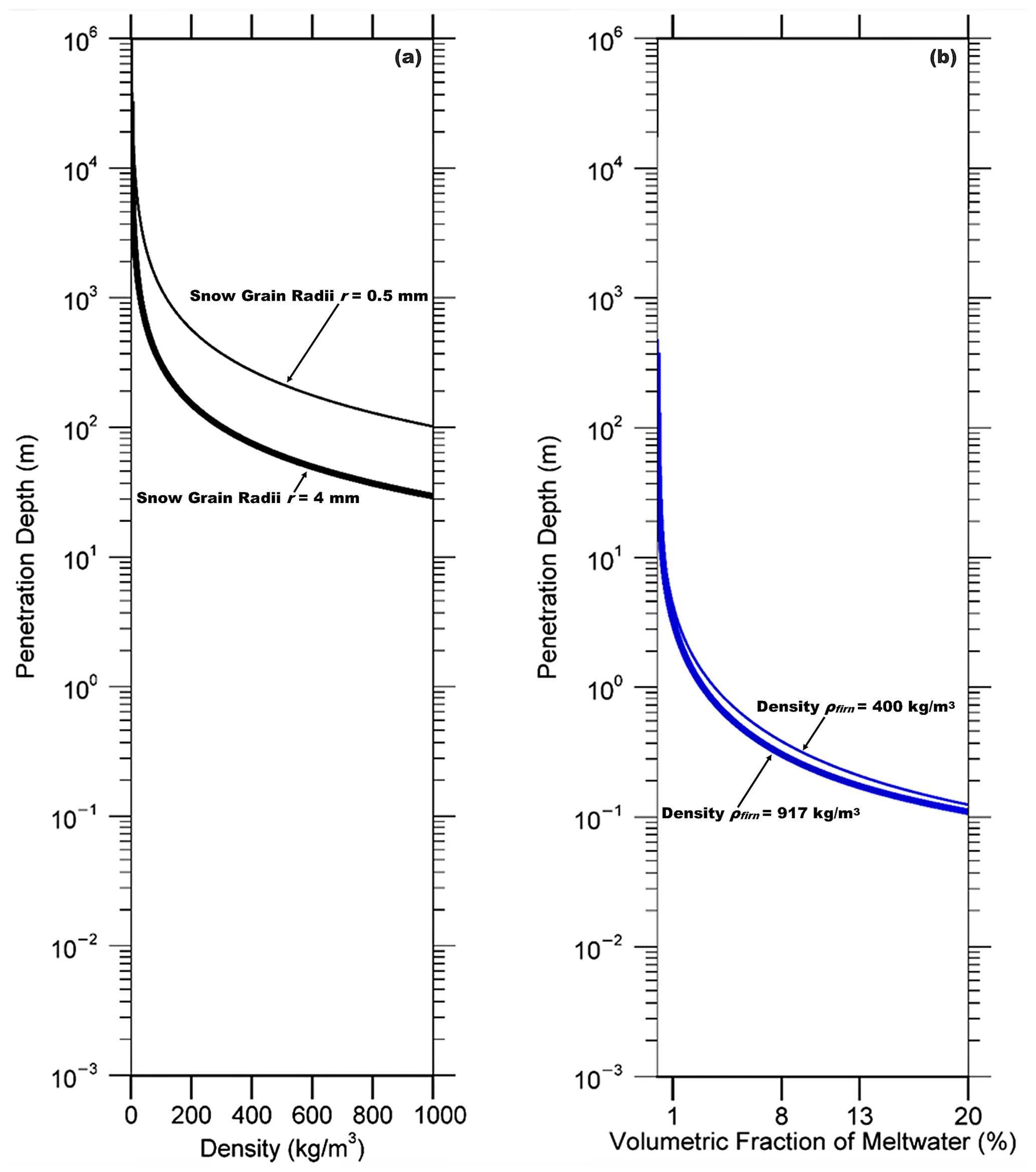
Figure 5 Theoretical L-band penetration depths for a uniform layer of (a) refrozen and (b) water-saturated firn. Penetration depths $(\mathrm{1}/({\mathit{\kappa }}_{\mathrm{s}}+{\mathit{\kappa }}_{\mathrm{a}}\left)\right)$ are calculated as a function of the Raleigh scattering coefficient (κ_s; Eq. 8) and the absorption coefficient (κ_a; Eq. 10). The complex dielectric constant is calculated using the empirically derived models described in Tiuri et al. (1984). Refrozen firn penetration depths are calculated as a function of firn density (ρ_firn), and the curves are plotted for snow grain radii (r) set to r=0.5 mm (upper curve) and r=4 mm (lower curve). Water-saturated firn penetration depths are calculated as a function of the volumetric fraction of meltwater (m_v), and the curves are plotted for firn density set to ρ_firn=400 kg m⁻³ (upper curve) and ρ_firn=917 kg m⁻³ (lower curve). Given the complexity of modeling embedded ice structures, they are excluded from the penetration depth calculation. Increases in the volumetric fraction of embedded ice within the firn will result in an increase in volume scattering, which will decrease and compress the distance between the penetration depth curves for both refrozen and water-saturated firn.

2.3.3 Continuous logistic model

We adapt our previously developed empirical algorithm to map the extent of Greenland's perennial firn aquifers (Miller et al., 2020) to also map the extent of ice slab areas. The empirical algorithm is derived from the continuous logistic model, which is based on a differential equation that models the decrease in physical systems as a function of time using a set of sigmoidal curves. These curves begin at a maximum value with an initial interval of decrease that is approximately exponential. Then, as the function approaches its minimum value, the decrease slows to approximately linear. Finally, as the function asymptotically reaches its minimum value, the decrease exponentially tails off and achieves stable values. We use the continuous logistic model to parametrize the refreezing rate within the water-saturated upper snow and firn layers of the percolation facies using $T_{\mathrm{V}}^{\mathrm{B}}$ time series that are partitioned using $T_{\text{V,max}}^{\mathrm{B}}$ and $T_{\text{V,min}}^{\mathrm{B}}$ values. We calculate the refreezing rate for each rSIR grid cell within the percolation facies extent as part of our adapted empirical algorithm (Sect. 2.3.4).

The continuous logistic model is described by a differential equation known as the logistic equation

$$\begin{array}{}\text{(3)}& {\displaystyle \frac{\mathrm{d}x}{\mathrm{d}t}}=\mathit{\zeta }x(\mathrm{1}-x)\end{array}$$

that has the solution

$$\begin{array}{}\text{(4)}& x\left(t\right)={\displaystyle \frac{\mathrm{1}}{\mathrm{1}+(\frac{\mathrm{1}}{x_o}-\mathrm{1})e^{-\mathit{\zeta }t}}},\end{array}$$

where x_o is the function's initial value, ζ is the function's exponential rate of decrease, and t is time. The function x(t) is also known as the sigmoid function. We use the sigmoid function to model the exponentially decreasing temporal L-band signatures observed over the percolation facies as a set of decreasing sigmoidal curves.

We first normalize $T_{\mathrm{V}}^{\mathrm{B}}$ time series for each rSIR grid cell

$$\begin{array}{}\text{(5)}& T_{\text{V,N}}^{\mathrm{B}}\left(t\right)={\displaystyle \frac{T_{\mathrm{V}}^{\mathrm{B}}\left(t\right)-T_{\text{V,min}}^{\mathrm{B}}}{T_{\text{V,max}}^{\mathrm{B}}-T_{\text{V,min}}^{\mathrm{B}}}},\end{array}$$

where $T_{\text{V,min}}^{\mathrm{B}}$ is the minimum vertically polarized L-band brightness temperature, and $T_{\text{V,max}}^{\mathrm{B}}$ is the maximum vertically polarized L-band brightness temperature. We then apply the sigmoid fit

$$\begin{array}{}\text{(6)}& T_{\text{V,N}}^{\mathrm{B}}\left(t\in [t_{\text{max}},t_{\text{min}}]\right)={\displaystyle \frac{\mathrm{1}}{\mathrm{1}+(\frac{\mathrm{1}}{T_{\text{V,N}}^{\mathrm{B}}\left(t_{\text{max}}\right)}-\mathrm{1})e^{-\mathit{\zeta }t}}}.\end{array}$$

$T_{\text{V,N}}^{\mathrm{B}}\left(t\in \left[t_{\text{max}},t_{\text{min}}\right]\right)$ is the normalized vertically polarized L-band brightness temperature on the time interval $t\in [t_{\text{max}},t_{\text{min}}]$, where t_max is the time the function achieves a maximum value, and t_min is the time the function achieves a minimum value. The initial normalized vertically polarized L-band brightness temperature ($T_{\text{V,N}}^{\mathrm{B}}\left(t_{\text{max}}\right)$) is the function's maximum value. The final normalized vertically polarized L-band brightness temperature ($T_{\text{V,N}}^{\mathrm{B}}\left(t_{\text{min}}\right)$) is the function's minimum value. The function's exponential rate of decrease represents the refreezing rate parameter (ζ). An example set of simulated sigmoidal curves is shown in Fig. 6.

Figure 6 Example set of simulated sigmoidal curves that represent our model of the exponentially decreasing temporal L-band signatures predicted over the percolation facies. The initial normalized vertically polarized L-band brightness temperature was fixed at a value of $T_{\text{V,N}}^{\mathrm{B}}\left(t_{\text{max}}\right)=\mathrm{0.99}$, and the time interval was set to a value of $t\in [t_{\text{max}},t_{\text{min}}]=\mathrm{300}$ observations. The refreezing rate parameter was set to values between $\mathit{\zeta }=[-\mathrm{1},\mathrm{0}]$ incremented by steps of 0.02. The blue lines correspond to the interval $\mathit{\zeta }\in [-\mathrm{0.04},-\mathrm{0.02}]$ and produce curves similar to those observed over perennial firn aquifer areas. The cyan lines correspond to the interval $\mathit{\zeta }\in [-\mathrm{0.06},-\mathrm{0.03}]$ and produce curves similar to those observed over ice slab areas. The black line is the observed lower bound ($\mathit{\zeta }=-\mathrm{0.09}$) of the refreezing rate parameter of partitioned $T_{\mathrm{V}}^{\mathrm{B}}$ time series iteratively fit to the sigmoid function (Sect. 2.3.4).

2.3.4 SMAP-derived extent mapping

Our adapted empirical algorithm is implemented in two steps: (1) mapping the extent of the percolation facies using the firn saturation parameter derived from the simple two-layer L-band brightness temperature model (Sect. 2.3.2) and (2) mapping the extent of perennial firn aquifer and ice slab areas over the percolation facies using the continuous logistic model (Sect. 2.3.3) we calibrate using airborne ice-penetrating radar surveys (Sect. 2.2).

Using Eq. (2), we first set a threshold for the firn saturation parameter (ξ_T) defined by the relationship

$$\begin{array}{}\text{(7)}& {\mathit{\xi }}_{\mathrm{T}}=({\mathit{\kappa }}_{\mathrm{s}}+{\mathit{\kappa }}_{\mathrm{a}})d\le \mathit{\xi }.\end{array}$$

We calculate the Raleigh scattering coefficient (κ_s) in Eq. (7) using

$$\begin{array}{}\text{(8)}& {\mathit{\kappa }}_{\mathrm{s}}=N_d{\displaystyle \frac{\mathrm{8}}{\mathrm{3}}}{k}_o^{\mathrm{4}}{r}^{\mathrm{6}}{\left|{\displaystyle \frac{{\mathit{\epsilon }}_r-\mathrm{1}}{{\mathit{\epsilon }}_r+\mathrm{2}}}\right|}^{\mathrm{2}},\end{array}$$

where N_d is the particle density, k_o is the wave number of the background medium of air, r is the snow grain radius set to r=2 mm, and ε_r is the complex dielectric constant. The particle density is defined by

$$\begin{array}{}\text{(9)}& N_d={\displaystyle \frac{{\mathit{\rho }}_{\text{firn}}}{{\mathit{\rho }}_{\text{ice}}}}{\displaystyle \frac{\mathrm{1}}{\frac{\mathrm{4}}{\mathrm{3}}\mathit{\pi }{r}^{\mathrm{3}}}},\end{array}$$

where ρ_firn is firn density set to ρ_firn=400 kg m⁻³, and ρ_ice is ice density set to ρ_ice=917 kg m⁻³. Our grain radius and firn density estimates are consistent with measurements within the upper snow and firn layers of the percolation facies of southeastern Greenland at the Helheim Glacier field site (Fig. 2a, blue circle), where in situ perennial firn aquifer measurements have recently been collected (Miller et al., 2017).

We calculate the absorption coefficient (κ_a) in Eq. (7) using

$$\begin{array}{}\text{(10)}& {\mathit{\kappa }}_{\mathrm{a}}=-\mathrm{2}{k}_o\mathfrak{I}\left\{\sqrt{{\mathit{\epsilon }}_r}\right\},\end{array}$$

where ℑ{ } represents the imaginary part. We calculate the complex dielectric constant of the water-saturated firn layer in Eqs. (8) and (10) using the empirically derived models described in Tiuri et al. (1984). We set the volumetric fraction of meltwater to m_v=1 %. We set the depth of the water-saturated firn layer in Eq. (7) to d=1 m. These values are consistent with typical lower frequency (e.g., 37, 13.4, 19 GHz) passive (e.g., Mote et al., 1995; Abdalati and Steffen, 1997; Ashcraft and Long, 2006) and active (e.g., Hicks and Long, 2011) microwave algorithms used to detect seasonal surface melting over the GrIS. Using the results of Eqs. (7–10), we calculate the firn saturation parameter threshold to be ξ_T=0.1.

The first step in our adapted empirical algorithm is to map the extent of the percolation facies. For each rSIR grid cell within the ice-masked extent of the GrIS, we smooth the corresponding $T_{\mathrm{V}}^{\mathrm{B}}$ time series using a 14-observation (1 week) moving window. We extract the minimum vertically polarized L-band brightness temperature ($T_{\text{V,min}}^{\mathrm{B}}$) and the maximum vertically polarized L-band brightness temperature ($T_{\text{V,max}}^{\mathrm{B}}$). We set the physical temperature of the water-saturated firn layer to T=273.15 K and the transmission angle to $\mathit{\theta }=\mathrm{40}{}^{\circ }$. We then calculate the firn saturation parameter (ξ) using Eq. (2). If the calculated firn saturation parameter exceeds the firn saturation parameter threshold, the rSIR grid cell is converted to a binary parameter to map the total extent of the percolation facies.

We note that smoothing $T_{\mathrm{V}}^{\mathrm{B}}$ time series will mask brief low-intensity seasonal surface melting that occurs in the high-elevation (>2500 m) percolation facies, where seasonal meltwater is rapidly refrozen within the colder snow and firn layers (e.g., Fig. 4d). Thus, the calculated firn saturation parameter will not exceed the firn saturation parameter threshold, and these rSIR grid cells are excluded from the algorithm. The exclusion of rSIR grid cells in the high-elevation percolation facies is not expected to have a significant impact on our results as our algorithm targets rSIR grid cells in areas that experience intense seasonal surface melting. The exclusion of rSIR grid cells may slightly underestimate the mapped percolation facies extent.

The second step in our adapted empirical algorithm is to map the extent of perennial firn aquifer and ice slab areas over the percolation facies. For each rSIR grid cell within the mapped percolation facies extent, we normalize the corresponding $T_{\mathrm{V}}^{\mathrm{B}}$ time series ($T_{\text{V,N}}^{\mathrm{B}}\left(t\right))$ using Eq. (5). We then extract the initial normalized vertically polarized L-band brightness temperature ($T_{\text{V,N}}^{\mathrm{B}}\left(t_{\text{max}}\right))$ and the final normalized vertically polarized L-band brightness temperature ($T_{\text{V,N}}^{\mathrm{B}}\left(t_{\text{min}}\right))$ and partition $T_{\text{V,N}}^{\mathrm{B}}\left(t\right)$ on the time interval $t\in [t_{\text{max}},t_{\text{min}}]$. We smooth $T_{\text{V,N}}^{\mathrm{B}}\left(t\in \left[t_{\text{max}},t_{\text{min}}\right]\right)$ using a 56-observation (4 week) moving window. The sigmoid fit is then iteratively applied using Eq. (6). Smoothing reduces the chi-squared error statistic when fitting $T_{\text{V,N}}^{\mathrm{B}}\left(t\in \left[t_{\text{max}},t_{\text{min}}\right]\right)$ to the sigmoid function. We fix the initial normalized vertically polarized L-band brightness temperature at $T_{\text{V,N}}^{\mathrm{B}}\left(t_{\text{max}}\right)=\mathrm{0.99}$, which provides a uniform parameter space in which the refreezing rate parameter (ζ) can be analyzed. Variability in $T_{\text{V,N}}^{\mathrm{B}}\left(t_{\text{max}}\right)$ is controlled by the volumetric fraction of meltwater within the upper snow and firn layers of the percolation facies and is accounted for in the firn saturation parameter (ξ), which is analyzed separately. $T_{\text{V,N}}^{\mathrm{B}}\left(t\in [t_{\text{max}},t_{\text{min}}]\right)$ values iteratively fit to the sigmoid function converge quickly (i.e., algorithm iterations $I\in [\mathrm{5},\mathrm{15}]$), and observations are a good fit (i.e., chi-squared error statistic is ${\mathit{\chi }}^{\mathrm{2}}\in [\mathrm{0},\mathrm{0.1}]$).

Using the SMAP-derived $T_{\text{V,N}}^{\mathrm{B}}\left(t_{\text{max}}\right)$ and $T_{\text{V,N}}^{\mathrm{B}}\left(t_{\text{min}}\right)$, rather than the MODIS-derived initial normalized vertically polarized L-band brightness temperature at the surface freeze-up date ($T_{\text{V,N}}^{\mathrm{B}}\left(t_{\text{sfu}}\right))$, and final normalized vertically polarized L-band brightness temperature at the melt onset date ($T_{\text{V,N}}^{\mathrm{B}}\left(t_{\text{mo}}\right)$) that were used in the empirical algorithm described in Miller et al. (2020), has several advantages. The key advantage of this approach is that maps can be generated using T^B imagery collected from a single satellite, which simplifies our adapted empirical algorithm. Another advantage is that unlike T^B collected at shorter-wavelength thermal infrared frequencies (e.g., MODIS), T^B collected at longer-wavelength microwave frequencies (e.g., SMAP) is not sensitive to clouds, which eliminates observational gaps and cloud contamination and provides more accurate time series partitioning and more robust curve fitting.

We calibrate our adapted empirical algorithm using the AR- and MCoRDS-derived perennial firn aquifer and ice slab detections projected on the NH EASE-Grid 2.0. For each rSIR grid cell with at least one detection, we extract the correlated maximum vertically polarized L-band brightness temperature ($T_{\text{V,max}}^{\mathrm{B}}$), the minimum vertically polarized L-band brightness temperature ($T_{\text{V,min}}^{\mathrm{B}}$), the firn saturation parameter (ξ), and the refreezing rate parameter (ζ). For each of the extracted calibration parameters, we calculate the standard deviation (σ). Thresholds of ±2σ are set in an attempt to eliminate peripheral rSIR grid cells near the ice sheet edge and near the boundaries of each sub-facies, where L-band emission can be influenced by morphological features, such as crevasses, and superimposed and glacial ice, and spatially integrated with emission from rock, land, the ocean, and adjacent percolation facies and wet snow facies areas. The calibration parameter intervals are given in Table 2. We apply the calibration to each rSIR grid cell within the percolation facies extent. If the extracted calibration parameters are within the intervals, the rSIR grid cell is converted to a binary parameter to map the total extent of each of these sub-facies.

Table 2 SMAP-derived calibration parameter intervals used for mapping perennial firn aquifer and ice slab extents.

Miller et al. (2020) cited significant uncertainty in the SMAP-derived perennial firn aquifer extent as a result of the lack of a distinct temporal L-band signature delineating the boundary between perennial firn aquifer areas and adjacent percolation facies areas. In this study, similar uncertainty exists in the SMAP-derived perennial firn aquifer and ice slab extents. This uncertainty could, at least in part, be a result of the rSIR algorithm. An rSIR grid cell corresponds to the weighted average of T^B over SMAP's antenna footprint (Long et al., 2019). The weighting is the grid cell's spatial response function (SRF), which is approximately 18 km (i.e., the effective resolution) in diameter. The SRF is centered on the rSIR grid cell. Since the effective resolution (i.e., the size of the 3 dB contour of the SRF) is greater than the rSIR grid cell spacing, the rSIR grid cell SRF's overlap and the T^B values are not statistically independent. This uncertainty, however, could also have a geophysical basis, as it is unlikely that the boundaries between sub-facies as well as between facies are distinct. The thickness of the water-saturated firn layer or ice slab may thin and taper off at the periphery, and sub-facies and facies may become spatially scattered and merge together.

The limited extent (AR, 15 m×20 m; MCoRDS, 14 m×40 m) of the airborne ice-penetrating radar surveys as compared to the rSIR grid cell extent (3.125 km) and the effective resolution of the SMAP enhanced-resolution $T_{\mathrm{V}}^{\mathrm{B}}$ imagery is also cited in Miller et al. (2020) as a source of uncertainty in the empirical algorithm. In this study, similar uncertainty exists in our adapted empirical algorithm. The total rSIR grid cell extent with airborne ice-penetrating radar survey coverage is less than 2 %. Thus, 98 % of the total rSIR grid cell extent from which the SMAP-derived calibration parameter intervals are extracted is unknown. Calculating the total rSIR grid cell extent where detections are absent along OIB flight lines and statistically integrating this calculation into the multi-year calibration technique may help reduce the uncertainty, particularly the significant uncertainty in the interannual variability in extent, which we have yet to resolve. A sensitivity analysis suggests that even small changes in the SMAP-derived calibration parameter intervals (i.e., several K for $T_{\text{V,min}}^{\mathrm{B}}$ and $T_{\text{V,max}}^{\mathrm{B}}$, several tenths of a percentage point for ξ, and several hundredths of a percentage point for ζ) can result in variability in the mapped extents of hundreds of square kilometers and boundary transitions between perennial firn aquifer and ice slab areas. Thus, the mapped extent of each of these sub-facies should simply be considered an initial result demonstrating the potential of our adapted empirical algorithm for future work.

3 Results and discussion

The SMAP-derived maximum vertically polarized L-band brightness temperature values generated by our adapted empirical algorithm range from between $T_{\text{V,max}}^{\mathrm{B}}=\mathrm{150}$ and 275 K, and the minimum vertically polarized L-band brightness temperature values range from between $T_{\text{V,min}}^{\mathrm{B}}=\mathrm{130}$ and 250 K. These values are consistent with the range of $T_{\text{V,max}}^{\mathrm{B}}$ and $T_{\text{V,min}}^{\mathrm{B}}$ values given in the temporal L-band signature analysis (Table 1). Firn saturation parameter values range from between ξ=0.1 and 4.0. Refreezing rate parameter values range from between $\mathit{\zeta }=-\mathrm{0.09}$ and −0.01. The observed lower bound ($\mathit{\zeta }=-\mathrm{0.09}$) of the refreezing rate parameter is significantly higher than the predicted lower bound ($\mathit{\zeta }=-\mathrm{1}$) in our example set of simulated sigmoidal curves (black line, Fig. 6).

The SMAP-derived perennial firn aquifer, ice slab, and percolation facies extents are shown in Figs. 7a–9a. The percolation facies extent (5.8×10⁵ km²) is mapped at elevations between 500 and 3000 m a.s.l. and extends over 32 % of the GrIS extent (1.8×10⁶ km²). The perennial firn aquifer extent (64 000 km²) is mapped at elevations between 600 and 2600 m a.s.l. and extends over 11 % of the percolation facies extent and 4 % of the GrIS extent. Predominately high $T_{\text{V,max}}^{\mathrm{B}}$, $T_{\text{V,min}}^{\mathrm{B}}$, ξ, and ζ values mapped within the perennial firn aquifer extent indicate the widespread presence of thicker water-saturated firn layers with larger volumetric fractions of meltwater that are radiometrically warm during both the melting and freezing seasons and have extended refreezing rates. The ice slab extent (76 000 km²) is mapped at elevations between 800 and 2700 m a.s.l. and extends over 13 % of the percolation facies extent and 4 % of the GrIS extent. As compared to perennial firn aquifer areas, decreased $T_{\text{V,max}}^{\mathrm{B}}$, $T_{\text{V,min}}^{\mathrm{B}}$, ξ, and ζ values in ice slab areas indicate the presence of thinner water-saturated firn layers with lower volumetric fractions of meltwater that are radiometrically colder and have slightly more rapid refreezing rates. Combined together, the total extent (140 000 km²) is the equivalent of 24 % of the percolation facies extent and 10 % of the GrIS extent. The extents of these sub-facies are generally isolated and somewhat scattered within the percolation facies. However, in several areas in south, south and central eastern, and northern Greenland, the sequential formation of sub-facies and facies (dry snow facies–percolation facies–ice slab–perennial firn aquifer–ablation facies) are mapped.

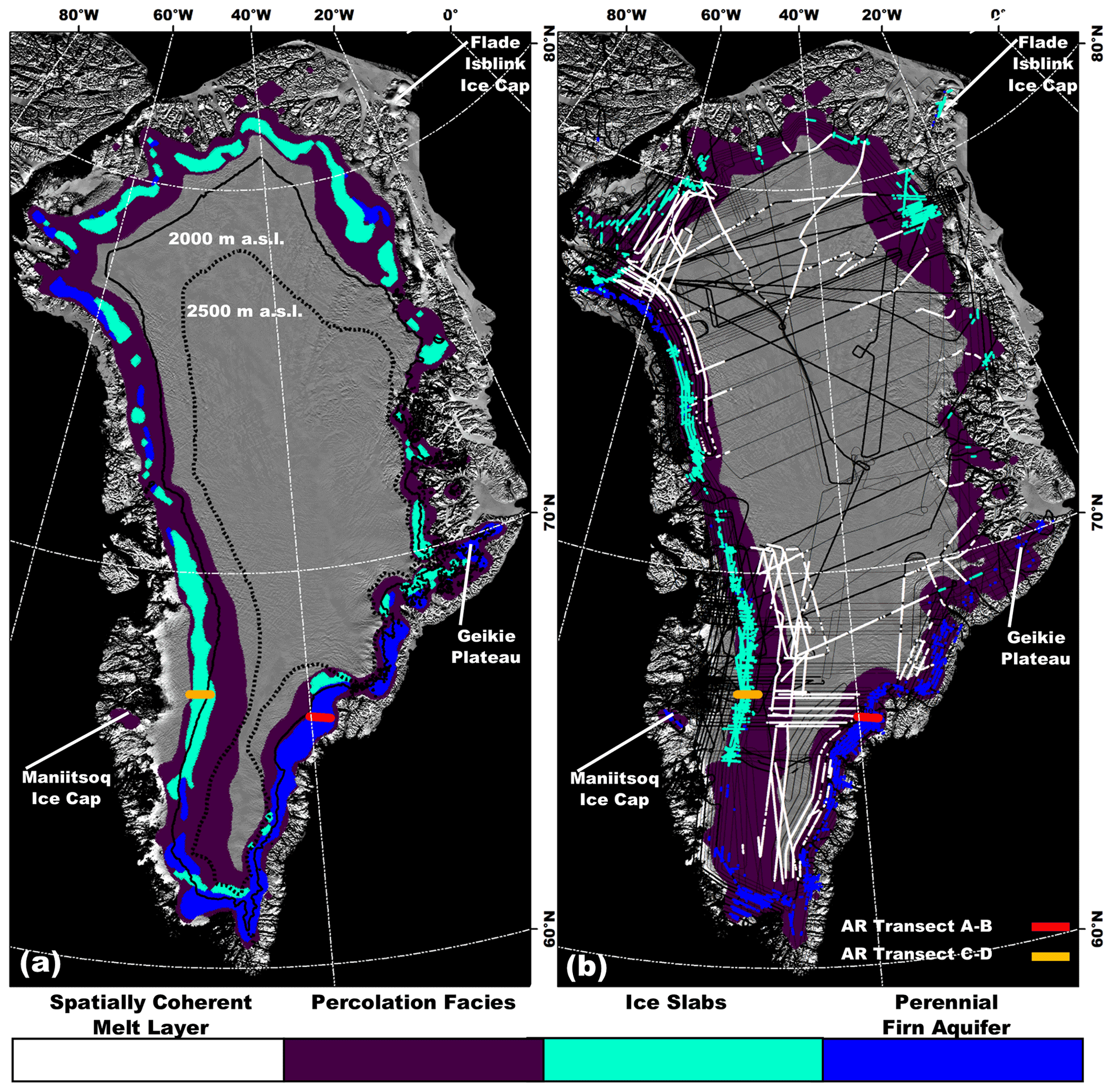
Figure 7 (a) SMAP-derived perennial firn aquifer (blue shading), ice slab (cyan shading), and percolation facies (purple shading) extents (2015–2019) generated by the adapted empirical algorithm as well as the 2000 m a.s.l. contour (black line) and the 2500 m a.s.l. contour (black dotted line; Howat et al., 2014) overlaid on the 2015 MODIS Mosaic of Greenland (MOG) image map (Haran et al., 2018). (b) SMAP-derived extents are overlaid with AR- and MCoRDS-derived 2010–2017 perennial firn aquifer (blue shading; Miège et al., 2016), 2010–2014 ice slab (cyan shading; MacFerrin et al., 2019), and 2012 spatially coherent melt layer (white shading; Culberg et al., 2021) detections along OIB flight lines (black interior lines); AR radargram transect A-B (red line; Fig. 3a) and C-D (orange line; Fig. 3b).

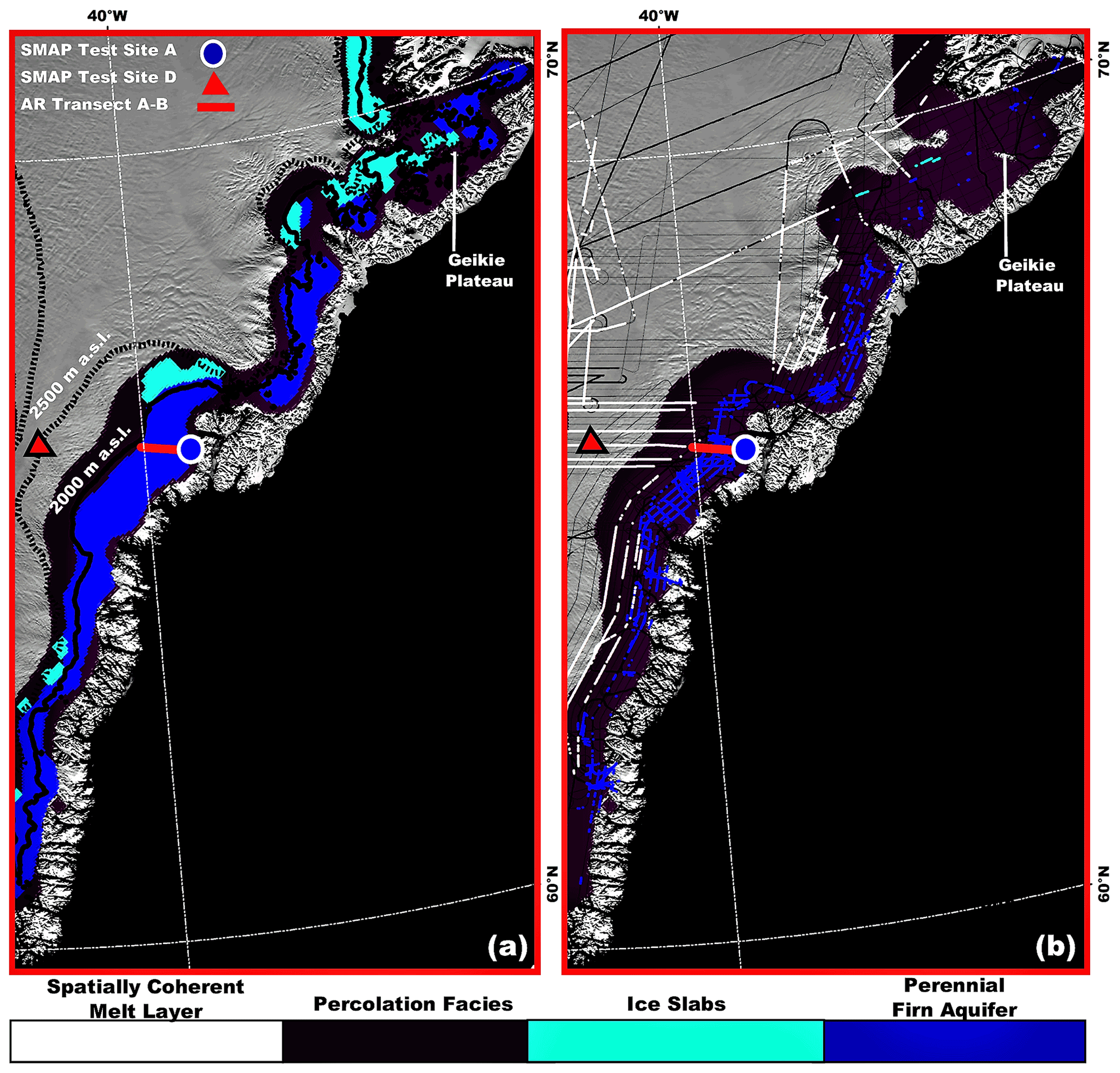
Figure 8 The SMAP-derived perennial firn aquifer (blue shading), ice slab (cyan shading), and percolation facies (purple shading) extents (2015–2019) generated by the adapted empirical algorithm over southeastern Greenland (red box; Fig. 1c) as well as the 2000 m a.s.l. contour (black line) and the 2500 m a.s.l. contour (black dotted line; Howat et al., 2014) overlaid on the 2015 MODIS MOG image map (Haran et al., 2018). (b) The SMAP-derived percolation facies extent is overlaid with AR- and MCoRDS-derived 2010–2017 perennial firn aquifer (blue shading; Miège et al., 2016), 2010–2014 ice slab (cyan shading; MacFerrin et al., 2019), and 2012 spatially coherent melt layer (white shading; Culberg et al., 2021) detections along OIB flight lines (black lines); AR radargram transect A-B (red line; Fig. 3a); and SMAP Test Site A (blue circle; Fig. 4a) and D (red triangle; Fig. 4d).

Figure 9 (a) SMAP-derived perennial firn aquifer (blue shading), ice slab (cyan shading), and percolation facies (purple shading) extents (2015–2019) generated by the adapted empirical algorithm over southwestern Greenland (orange box; Fig. 1c) as well as the 2000 m a.s.l. contour (black line) and the 2500 m a.s.l. contour (black dotted line; Howat et al., 2014) overlaid on the 2015 MODIS MOG image map (Haran et al., 2018). (b) SMAP-derived percolation facies extent is overlaid with AR- and MCoRDS-derived 2010–2017 perennial firn aquifer (blue shading; Miège et al., 2016), 2010–2014 ice slab (cyan shading; MacFerrin et al., 2019), and 2012 spatially coherent melt layer (white shading; Culberg et al., 2021) detections along OIB flight lines (black interior lines); AR radargram transect C-D (orange line; Fig. 3b); and SMAP Test Site B (cyan circle; Fig. 4b), C (orange diamond; Fig. 4c), and E (yellow circle; Fig. 4e).

Figures 7b–9b show perennial firn aquifers, ice slabs, and spatially coherent melt layers detected by airborne ice-penetrating radar surveys overlaid on the SMAP-derived percolation facies extent. The SMAP-derived perennial firn aquifer extent mapped in southern as well as south and central eastern Greenland is consistent with the AR- and MCoRDS-derived perennial firn aquifer detections. Additional smaller perennial firn aquifer areas are mapped in northern Greenland. The SMAP-derived ice slab extent mapped in southwestern and central eastern Greenland is generally consistent with the spatial patterns of the AR-derived ice slab detections but is significantly expanded upslope in each of these areas. In northern Greenland, perennial firn aquifers areas are alternatively mapped, and additional expansive ice slab areas are mapped upslope of perennial firn aquifer areas. Additional smaller ice slab areas are mapped in south and southeastern Greenland. We note that the AR- and MCoRDS-derived perennial firn aquifer and ice slab detections are limited in space and time, particularly in northern Greenland, with a time interval as large as 9 years between the airborne ice-penetrating radar surveys and the SMAP enhanced-resolution $T_{\mathrm{V}}^{\mathrm{B}}$ imagery we use in our adapted empirical algorithm. In western and northern Greenland, the 2015 melting season was especially intense (Tedesco et al., 2016). And, in northern Greenland, the ablation facies have recently (2010–2019) increased in extent (Noël et al., 2019), and supraglacial lakes have recently (2014–2019) advanced inland (Turton et al., 2021), indicating a possible geophysical basis for the observed formation, boundary transitions, and expansion. Neither perennial firn aquifer nor ice slab areas are mapped on the Maniitsoq and Flade Isblink ice caps, where spatially integrated L-band emission results in calibration parameter values outside the defined intervals for each of these sub-facies.

Although the AR-derived spatially coherent melt layer detections are often observed to be adjacent to perennial firn aquifer and ice slab areas, these sub-facies were masked in the original airborne ice-penetrating radar survey analysis by Culberg et al. (2021). Spatially coherent melt layers often overlay perennial firn aquifers (e.g., Fig. 3a) and merge with ice slabs (Culberg et al., 2021; Fig. 4).

Shallow buried supraglacial lakes have recently been identified within the percolation facies of western, northern, and north and central eastern Greenland using airborne ice-penetrating radar surveys (Koenig et al., 2015) and satellite synthetic aperture radar imagery (Miles et al., 2017; Schröder et al., 2020; Dunmire et al., 2021). These buried supraglacial lakes are within the SMAP-derived perennial firn aquifer and ice slab extents but are not expected to significantly influence L-band emission in these areas for two reasons. (1) As compared to SMAP's 18 km effective resolution, the mean extent of buried supraglacial lakes is limited (less than 1 km²), and they are sparsely distributed in perennial firn aquifer and ice slab areas (Dunmire et al., 2021). (2) Supraglacial lakes form during the melting season as a result of meltwater storage within topographic depressions at the ice sheet surface (Echelmeyer et al., 1991). Similar to subglacial lakes (Jezek et al., 2015) and perennial firn aquifers (Miller et al., 2020), supraglacial lakes represent radiometrically cold near-surface meltwater reservoirs. Upwelling L-band emission from deeper firn layers, superimposed and/or glacial ice, and the underlying bedrock are effectively blocked by high reflectivity and attenuation at the interface between the lake bottom and the underlying impermeable layer. This results in low observed T^B at the upper surface of meltwater stored within supraglacial lakes. During the freezing season, the upper surface of meltwater refreezes and forms a partial or solid-ice cap that is sometimes buried by snow accumulation (Koenig et al., 2015). Airborne ice-penetrating radar surveys in April and May between 2009 and 2012 suggest the mean depth to the upper surface of meltwater stored within buried supraglacial lakes is approximately 2 m (Koenig et al., 2015). Over buried supraglacial lakes, L-band emission from the refreezing partial or solid-ice cap, which is smooth relative to the L-band wavelength (21 cm), likely induces surface scattering. As a result, $T_{\mathrm{V}}^{\mathrm{B}}$ decreases over buried supraglacial lakes are likely negligible. Thus, over SMAP's 18 km effective resolution, we postulate water-saturated firn layers dominate L-band emission over the percolation facies of the GrIS.

The SMAP-derived perennial firn aquifer extent (64 000 km²) generated by our adapted empirical algorithm and the multi-year calibration technique (2015–2019) is consistent with the extent (66 000 km²) generated by the previously developed empirical algorithm and the single-coincident year calibration technique (2016) described in Miller et al. (2020). The SMAP-derived perennial firn aquifer extent is generally consistent with previous C-band (5.3 GHz) satellite-radar-scatterometer-derived perennial firn aquifer extents mapped using the Advanced SCATterometer (ASCAT) on the European Organization for the Exploitation of Meteorological Satellites (EUMETSAT) Meteorological Operational A (MetOp-A) satellite (2009–2016, 52 000–153 000 km²; Miller, 2019) and the Active Microwave Instrument in radar scatterometer mode (ESCAT) on ESA's European Remote Sensing (ERS) satellite series (1992–2001, 37 000–64 000 km²; Miller, 2019) as well as the C-band (5.4 GHz) synthetic-aperture-radar-derived extent mapped using ESA's Sentinel-1 satellite (2014–2019, 54 000 km²; Brangers et al., 2020). The exception is the ASCAT-derived perennial firn aquifer extent (2012–2013, 153 000 km²; Miller, 2019) mapped following the 2012 melting season (Nghiem et al., 2012) in which significant changes in the dielectric and geophysical properties that influence radar backscatter likely occurred. The unreasonably expansive (i.e., more than twice the mean) mapped extent is a result of ASCAT's shallow (several meters) C-band penetration depth (Jezek et al., 1994) and the simple threshold-based algorithm, which was not calibrated for an extreme melting season that included saturation of the upper snow and firn layers of the dry snow facies and percolation facies with relatively large volumetric fractions of meltwater (Miller et al., 2019). Water-saturated firn layers had extended refreezing rates; however, seasonal meltwater was not stored at depth. Widespread spatially coherent melt layers were alternatively formed in many of the mapped areas (Culberg et al., 2021). The SMAP-derived ice slab extent (76 000 km²) is also consistent with previous AR-derived ice slab extents (2010–2014, 64 800–69 400 km²; MacFerrin et al., 2019).

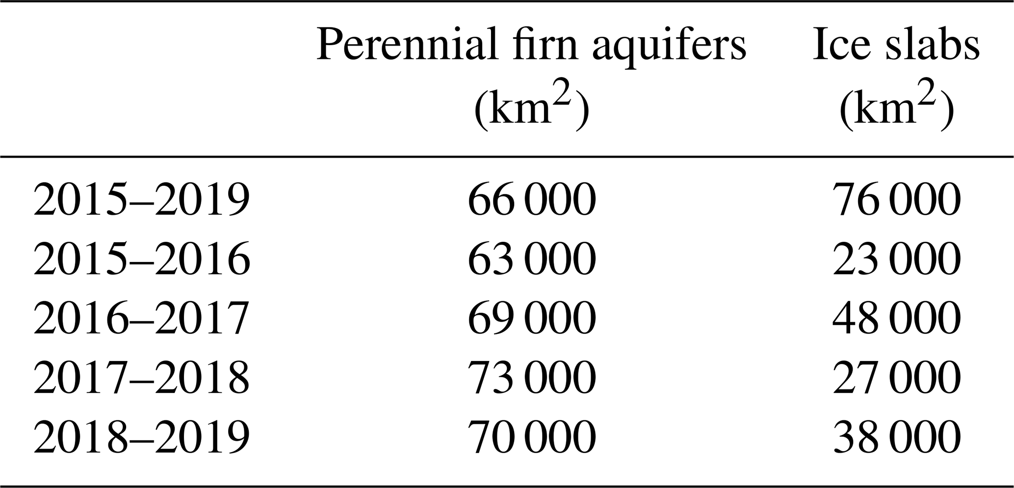
Although we simply consider our mapped extents a high-probability area for preferential formation, the maps generated by our adapted empirical algorithm and the multi-year calibration technique for individual years suggest there is reasonable interannual variability in perennial firn aquifer and ice slab extents (Table 3). Our results demonstrate sensitivity to variability in the depth- and time-integrated dielectric and geophysical properties of the percolation facies that influence the radiometric temperature, even during the 2015 melting season (Tedesco et al., 2016).

Table 3 Interannual variability in SMAP-derived perennial firn aquifer and ice slab extents.

4 Implications

Seasonal surface melting over the GrIS has increased in extent, intensity, and duration since early in the satellite era (Steffen et al., 2004; Tedesco et al., 2008, 2011, 2016; Nghiem et al., 2012; Tedesco and Fettweis, 2020; Cullather et al., 2020). Consistent with recent seasonal surface melting trends, meltwater runoff has accelerated to become the dominant mass loss mechanism over the GrIS (van den Broeke et al., 2016). Meltwater storage in both solid (i.e., embedded ice structures, including ice slabs, and spatially coherent melt layers) and liquid (i.e., perennial firn aquifers) form can buffer meltwater runoff in the percolation facies and delay its eventual release into the ocean (Harper et al., 2012). However, significant uncertainty remains in meltwater runoff estimates as a result of the lack of knowledge of heterogeneous infiltration and refreezing processes within the snow and firn layers (Pfeffer and Humphrey, 1996) as well as the depths to which meltwater can descend beneath the ice sheet surface (Humphrey et al., 2012).

If the increasing seasonal surface melting trend continues (Franco et al., 2013; Noël et al., 2021), perennial firn aquifer formation and expansion may increase the possibility of crevasse deepening via meltwater-induced hydrofracturing (Alley et al., 2005; van der Veen, 2007), especially if crevasse fields expand into perennial firn aquifer areas as a result of accelerated ice flow (Colgan et al., 2016). Meltwater-induced hydrofracturing is an important component of supraglacial lake drainage during the melting season (Das et al., 2008; Stevens et al., 2015), leading to at least temporary localized accelerated ice flow velocities (Zwally et al., 2002; Joughin et al., 2013; Moon et al., 2014) as well as ice discharge from outlet glaciers (Chudley et al., 2019) and mass balance changes (Joughin et al., 2008). Perennial firn aquifers may also support meltwater-induced hydrofracturing, even during the freezing season (Poinar et al., 2017, 2019).

The formation and expansion of ice slabs reduces permeability within the upper snow and firn layers and facilitates lateral meltwater flow with minimum vertical percolation into the deeper firn layers, thereby enhancing meltwater runoff and mass loss at the periphery (Machguth et al., 2016; MacFerrin et al., 2019). Lateral meltwater flow across ice layers overlying deeper permeable firn layers was first postulated by Müller (1962). The theory was then further developed by Pfeffer et al. (1991) as an end-member case for meltwater runoff in the percolation facies, with the other end-member case being lateral meltwater flow across superimposed ice. Lateral meltwater flow and high-elevation (1850 m a.s.l.) meltwater runoff across ice slabs in the percolation facies were first observed in visible satellite imagery collected by the NASA–USGS Landsat 7 mission during the 2012 melting season (Machguth et al., 2016).

Spatially coherent melt layers represent a recently identified refreezing mechanism in the dry snow facies (Nghiem et al., 2005; Culberg et al., 2021). Similar to ice slabs, the formation and expansion of spatially coherent melt layers reduce the pore space within the upper snow and firn layers. They can also limit meltwater flow with minimum vertical percolation into the deeper firn layers, thereby potentially preconditioning the dry snow facies for the formation of ice slabs and enhanced meltwater runoff from significantly higher elevations on accelerated timescales. If spatially coherent melt layers merge with ice slabs upslope of perennial firn aquifers areas, they may also simultaneously accelerate both meltwater runoff and meltwater-induced hydrofracturing during extreme melting seasons. The formation of spatially coherent melt layers overlying deeper perennial firn aquifers may result in the formation of shallow perched firn aquifers (Culberg et al., 2021) or may terminate gravity-driven meltwater drainage and seasonal recharging (Fountain and Walder, 1998), which may eventually completely refreeze stored meltwater into ice slabs or decameters-thick solid-ice layers overlying deeper glacial ice.

5 Summary and future work

In this study, for the first time, we have demonstrated the novel use of the L-band microwave radiometer on NASA's SMAP satellite for mapping perennial firn aquifers and ice slabs together as a continuous englacial hydrological system over the percolation facies of the GrIS. We have adapted our previously developed empirical algorithm (Miller et al., 2020) by expanding our analysis of spatiotemporal differences in SMAP enhanced-resolution $T_{\mathrm{V}}^{\mathrm{B}}$ imagery and temporal L-band signatures. We have used this analysis to derive a firn saturation parameter from a simple two-layer L-band brightness temperature model. And we have used the firn saturation parameter to map the extent of the percolation facies. We have found that by correlating maximum and minimum $T_{\mathrm{V}}^{\mathrm{B}}$ values, the firn saturation parameter, and the refreezing rate parameter with perennial firn aquifer and ice slab detections identified via the CReSIS AR and MCoRDS instruments flown by NASA's OIB campaigns, we can calibrate our previously developed empirical algorithm (Miller et al., 2020) to map plausible extents.

We note that significant uncertainty exists in the mapped extents as a result of (1) correlating the SMAP-derived parameters with airborne ice-penetrating radar detections that are not coincident in time; (2) the lack of a distinct temporal L-band signature delineating the boundary between perennial firn aquifer areas, ice slabs areas, and adjacent percolation facies areas; and (3) the limited extent of the airborne ice-penetrating radar detections as compared to the rSIR grid cell extent and the effective resolution of the SMAP enhanced-resolution $T_{\mathrm{V}}^{\mathrm{B}}$ imagery.

Miller et al. (2020) normalized SMAP enhanced-resolution $T_{\mathrm{V}}^{\mathrm{B}}$ time series and converted the exponential rate of $T_{\mathrm{V}}^{\mathrm{B}}$ decrease over perennial firn aquifer areas to a binary parameter to map extent. In this study, we have converted the SMAP-derived parameters to binary parameters to map the extent of both perennial firn aquifer and ice slab areas. Moreover, we have included additional analysis of the spatiotemporal differences in maximum and minimum $T_{\mathrm{V}}^{\mathrm{B}}$ values, the firn saturation parameter, and the refreezing rate parameter. We have shown that spatiotemporal differences in the SMAP-derived parameters are consistent with our assumption of spatiotemporal differences in the englacial hydrology and thermal characteristics of firn layers at depth.

Future work will focus on simulating the temporal L-band signatures observed over perennial firn aquifer and ice slab areas for a wide range of geophysical properties. Additionally, we will simulate the distinct temporal L-band signatures observed over spatially coherent melt layers and explore mapping the extent. Combining multi-layer depth-integrated L-band brightness temperature models (e.g., Jezek et al., 2015) that include embedded ice structure parametrizations (e.g., Jezek et al., 2018) with models of depth-dependent geophysical parameters can lead to an improved understanding of the extremely complex and poorly described physics controlling L-band emission over the percolation facies. The development of more sophisticated empirical algorithms that incorporate multi-layer depth-integrated L-band brightness temperature models that are constrained by in situ measurements can help reduce the significant uncertainty in the current mapped extents and provide more accurate boundary delineation that can be used to further quantify interannual variability.