the Creative Commons Attribution 4.0 License.
the Creative Commons Attribution 4.0 License.
 | 17 Dec 2021
Seasonal evolution of basal environment conditions of Russell sector, West Greenland, inverted from satellite observation of surface flow
Anna Derkacheva
Fabien Gillet-Chaulet
Jeremie Mouginot
Eliot Jager
Nathan Maier
Samuel Cook
Due to increasing surface melting on the Greenland ice sheet, better constraints on seasonally evolving basal water pressure and sliding speed are required by models. Here we assess the potential of using inverse methods on a dense time series of surface speeds to recover the seasonal evolution of the basal conditions in a well-documented region in southwest Greenland. Using data compiled from multiple satellite missions, we document seasonally evolving surface velocities with a temporal resolution of 2 weeks between 2015 and 2019. We then apply the inverse control method using the ice flow model Elmer/Ice to infer the basal sliding and friction corresponding to each of the 24 surface velocity data sets. Near the margin where the uncertainty in the velocity and bed topography are small, we obtain clear seasonal variations that can be mostly interpreted in terms of an effective-pressure-based hard-bed friction law. We find for valley bottoms or “troughs” in the bed topography that the changes in modelled basal conditions directly respond to local modelled water pressure variations, while the link is more complex for subglacial “ridges” which are often non-locally forced. At the catchment scale, in-phase variations in the water pressure, surface velocities, and surface runoff variations are found. Our results show that time series inversions of observed surface velocities can be used to understand the evolution of basal conditions over different timescales and could therefore serve as an intermediate validation for subglacial hydrology models to achieve better coupling with ice flow models.
- Article
(14254 KB) - Full-text XML
- BibTeX
- EndNote


In recent decades, the Greenland ice sheet (GrIS) has been losing mass, reaching a negative mass balance of about Gt yr−1 in 2010–2018 (Mouginot et al., 2019). An important part of this loss comes from the ice-discharge acceleration of tidewater glaciers. In addition, ice dynamics also plays a significant role in land-terminating sectors as ice flow affects the flux of ice into the ablation area and the ice-sheet topography, with feedbacks between ice-sheet surface elevation and the atmosphere that can enhance mass loss in century-scale projections (Edwards et al., 2014; Le Clec'h et al., 2019).
Water pressure at the glacier base is considered to be a major control on basal sliding that affects ice dynamics over different timescales (Nienow et al., 2017; Davison et al., 2019). For instance, seasonal modulations of water input to the bed, induced by summer melt, are able to lead to peak glacier accelerations of up to +360 % locally compared to winter mean velocities (Palmer et al., 2011). Increased water pressure as melt drains through an inefficient drainage system is assumed by existing theories to be the mechanism driving the acceleration during the beginning of the melt season. However, increased drainage efficiency during the late melt season leads to a decrease in water pressures and causes a commensurate glacier deceleration. Moreover, during high melt years, higher early summer velocities are therefore supposed to be responsible for the slower velocities during the late melt and winter seasons, offsetting the higher initial ice flux (Tedstone et al., 2015). This suggests that the future of the GrIS will likely be affected by the evolution of the surface runoff discharge and its effect on the subglacial drainage system.
The rate of surface melting is already increasing due to warming of the air, as well as other factors amplifying this phenomenon such as the decrease in ice albedo (Box et al., 2012), decrease in the capacity of the firn to retain meltwater (Mikkelsen et al., 2016), or even change in the dominant weather type (Van Tricht et al., 2016). Climate models predict that this melting will continue to grow in the future. Surface runoff is also increasing in both observations and projection models (Ahlstrøm et al., 2017; Trusel et al., 2018). However, it is still debated how the ice flow velocity will respond to this enhancement in water production in the long term: with a continuous increase (Zwally et al., 2002; Greskowiak, 2014; Hewitt, 2013), an increase until a threshold (Tedstone et al., 2013, 2014; Poinar et al., 2015), or even a decrease (Tedstone et al., 2015; Stevens et al., 2016). A complete analysis of all these hypotheses suggests that different trends will dominate according to the timescale and altitudes considered (Nienow et al., 2017; Davison et al., 2019).
These questions have motivated the development of physical models to represent the subglacial environment and its interaction with ice dynamics. Basic ingredients of these models are (i) a subglacial hydrological model that computes effective pressure and (ii) a friction law that relates basal shear stress to the effective pressure and the basal sliding velocity. However, because of the limited accessibility to the basal environment, the processes at the bed remain difficult to characterize, limiting their understanding. Both components are still a matter of debate, and no consensus has emerged.
Flowers (2015) gives a review of available subglacial hydrology models and their theoretical background. A total of 13 models of various complexity have participated in a recent model intercomparison exercise that shows that physical approaches coupling several elements of the basal drainage system significantly differ from simpler approaches for short term, e.g. diurnal, variations (De Fleurian et al., 2018). To be run operationally, these physical models require highly detailed input data (e.g. basal topography, runoff forcing) that are often not available, and they suffer from a lack of direct and independent data for calibration and validation. The most direct way to access the basal hydrology system is to drill boreholes that allow direct measurements of the water pressure (Smeets et al., 2012; Meierbachtol et al., 2013; Van De Wal et al., 2015; Wright et al., 2016). While very valuable, these local measurements can show a high spatial variability depending on the element of the basal hydrology (e.g. active or inactive part of the subglacial drainage system) that is sampled (Wright et al., 2016), so these observations make the validation of subglacial hydrology models challenging, as they are not necessarily representative of the large-scale average basal conditions that are required to reproduce and predict the long-term evolution of the entire glacier. However, basal hydrology models have been applied in real settings, and the comparison with available observations has stimulated their development. For instance, in de Fleurian et al. (2016) the timing of the response of modelled water pressure broadly agrees with observations but with a significant difference in terms of magnitude. In addition to an efficient and inefficient drainage system, Hoffman et al. (2016) introduced a third weakly connected component to explain the decline of water pressure during the late melt season. Alternatively, Downs et al. (2018) suggest a reduction in hydraulic conductivity to explain the tendency of models to underpredict observed winter water pressure.
The second required component, the friction law, depends on the properties of the bed. Deformable basal sediments (commonly referred to as soft or weak beds) are usually modelled using a Mohr–Coulomb criterion to relate the basal shear stress to the effective pressure (Iverson et al., 1998; Fowler, 2003; Joughin et al., 2019; Helanow et al., 2021). For hard beds (rigid rocks or non-deformable till, as opposed to deformable till), the friction is controlled by the ice deformation over the small-scale basal roughness, inducing a relationship between the basal shear stress and the sliding velocity. Increasing the water pressure can open subglacial cavities, reducing the apparent bed roughness and the basal friction (also referred to as basal shear stress or basal traction). Several friction laws that incorporate the dependency on effective pressure have thus been developed from both theoretical (Schoof, 2005) and empirical considerations (Budd et al., 1984). Because of the inaccessibility of the basal environment, the bed properties of specific glaciers are generally poorly known. Additionally, geophysical investigations have shown evidence for the presence of deformable sediments and hard beds in relatively close proximity (Dow et al., 2013; Harper et al., 2017). Thus, in situ direct validation of the friction law is not possible, so models must be evaluated against surface velocities, necessarily inducing uncertainties in the basal hydrology and ice deformation.
Synthetic simulations of typical Greenlandic land-terminating glaciers using coupled basal hydrology–ice dynamics models have been able to reproduce the main observed features of the seasonal modulation of surface velocity (Hewitt, 2013; Gagliardini and Werder, 2018; Cook et al., 2020). Models have mostly been validated using velocity fluctuations recorded by GPS at the ice-sheet surface (Bougamont et al., 2014; Kulessa et al., 2017; Christoffersen et al., 2018; Koziol and Arnold, 2018). Again, being precise, these measurements are local and do not allow the spatial variability of the processes to be properly constrained.
Satellite imagery allows us to derive surface velocity fields with a good spatial resolution and coverage. During the last decade, the number of such observations has increased significantly with the launches of missions such as Landsat-8 or Sentinel-1 and Sentinel-2 (Fahnestock et al., 2016; Mouginot et al., 2017; Joughin et al., 2018; Lemos et al., 2018), allowing the reconstruction of flow variations at the seasonal scale with a temporal resolution of days to weeks (Altena and Kääb, 2017; Vijay et al., 2019; Derkacheva et al., 2020).
Most recent ice flow models now include various inverse methods that make it possible to spatially constrain a free parameter that relates the basal friction to the sliding velocity using the observed geometry and surface velocity field (MacAyeal, 1993; Arthern and Gudmundsson, 2010). Several studies have then tried to validate or constrain the friction law from the inferred basal friction and velocity. As the velocities in ice sheets can range over several orders of magnitude, this can be assessed from the spatial variations in a single inversion, assuming that changes are mostly driven by the friction law and not by spatial variations in the bed properties. Thus, Arthern et al. (2015) found that the basal stress in Antarctica, on average, roughly agrees with a uniform value of ∼100 kPa; however this can change locally by orders of magnitude. Spatially aggregating inversions with models of different complexity, Maier et al. (2021a) found that large areas under the Greenland ice sheet broadly agree with hard-bed physics. The other possibility to constrain the friction law is to use several inversions to study the temporal changes; however this can be done only where the changes are sufficiently large. For instance, Gillet-Chaulet et al. (2016) found that changes in the drainage basin of Pine Island Glacier in Antarctica over a 14-year period can be explained with a mostly plastic relation, where the basal friction is weakly sensitive to changes in sliding velocity.
Temporal variations in basal hydrology have been addressed by several studies using inferred velocity fields to constrain temporal variations in the basal water pressure by assuming a certain friction law that also includes effective pressure (Jay-Allemand et al., 2011; Minchew et al., 2016). The main objective of this paper is to assess the ability of existing inverse methods to use satellite-derived seasonal velocity maps to infer seasonal variations in the basal conditions.
We focus on a land-terminating sector of the southwest coast of Greenland located at 67∘ N, 50∘ E. This sector includes a slow-moving ice-sheet margin and three distinct glaciers (from north to south): Insunnguata Sermia, Russell Glacier, and Ørkendalen Gletscher (Fig. 1). Hereafter, this area is referred to as the Russell sector. Extensive measurements of the ice thickness were carried out over the study region using radar sounders, especially through NASA's Operation IceBridge mission (Morlighem et al., 2013; Lindbäck et al., 2014). This dense data set with an average radar-line spacing of less than 500 m is exceptional by Greenland standards, where most radar lines are generally separated by tens of kilometres. In addition, because of its relative accessibility, this sector has been the subject of numerous complementary geophysical investigations such as boreholes, seismometers, or GPS (Smeets et al., 2012; Dow et al., 2013; Wright et al., 2016; Harper et al., 2017; Kulessa et al., 2017; Maier et al., 2019), making it a privileged study site for numerical investigations (Bougamont et al., 2014; de Fleurian et al., 2016; Koziol and Arnold, 2017, 2018; Downs et al., 2018; Christoffersen et al., 2018; Brinkerhoff et al., 2021).
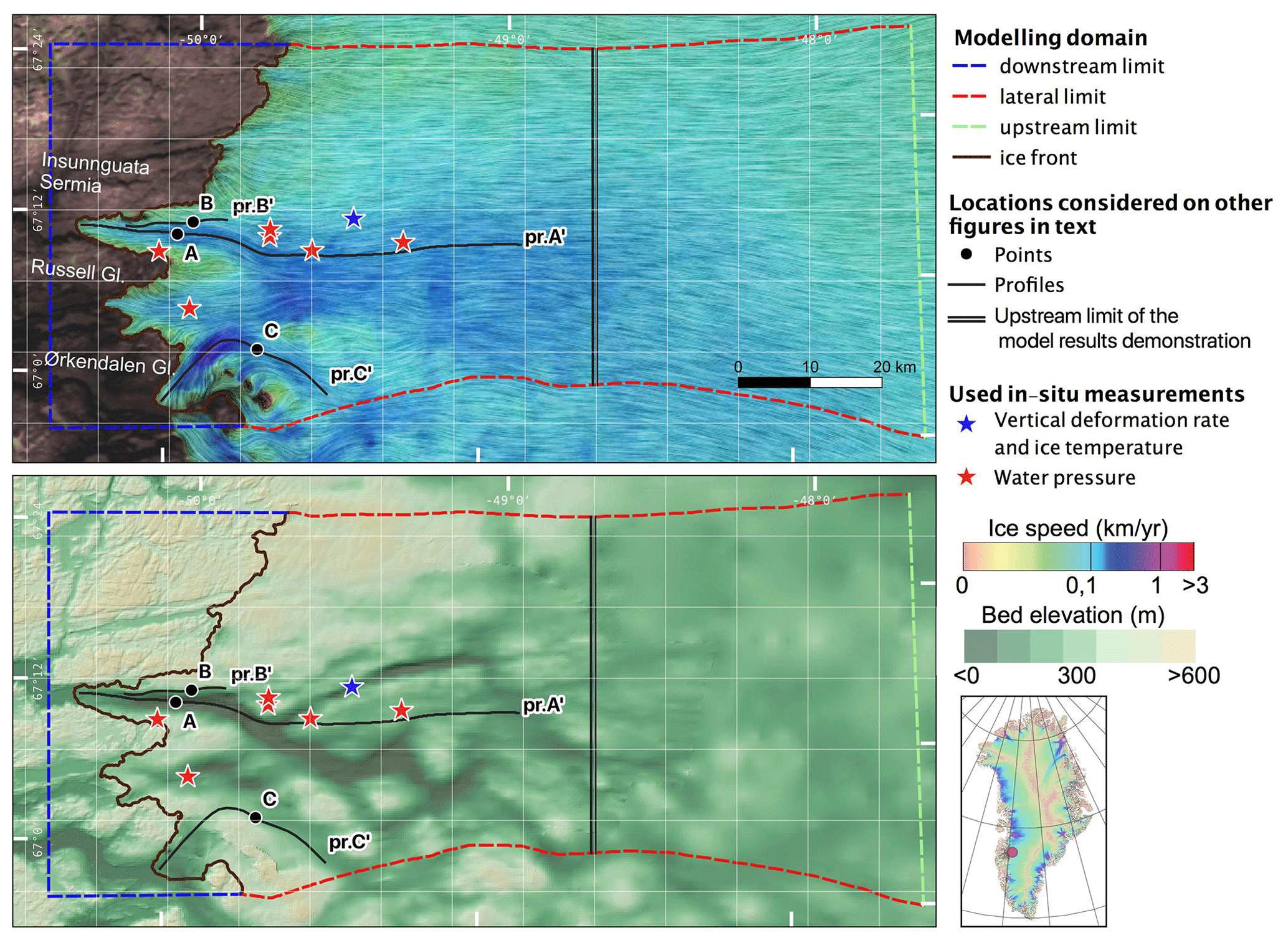
Figure 1Study area with modelling domain. The points (A–C) and profiles (pr. A', pr. C') indicate locations considered later in the text, and the blue and red stars indicate locations of in situ measurements (Smeets et al., 2012; Meierbachtol et al., 2013; Wright et al., 2016; Hills et al., 2017; Maier et al., 2019). The top panel shows the surface ice velocity overlaid on the line integral convolution (Cabral and Leedom, 1993) to visualize the flow vector direction (Mouginot et al., 2017). The bottom panel displays the bed elevation from BedMachine (Morlighem et al., 2017). The white 10 km grid used here is identical in all figures in the article. The projection used is polar stereographic north with latitude of true scale at 70∘ N.
We use the three-dimensional finite-element full-Stokes ice flow model Elmer/Ice (Gagliardini et al., 2013) to invert for the seasonal evolution of the basal friction and sliding speed using surface velocity maps covering an entire year with a time step of 2 weeks. We address how best to integrate satellite-derived velocity into a model, as well as the sensitivity of the inverted basal friction fields to initial ice temperature and some commonly used model parameters. From the inverted basal fields, we estimate the corresponding evolution of the water pressure using a pressure-dependent friction law (Schoof, 2005; Gagliardini et al., 2007). Results are discussed using available in situ measurements and outputs from numerical models of subglacial hydrology and regional climate. Finally, we conclude with the usability of inverse-flow models with spatio-temporally dense observations of surface velocity to derive the seasonal evolution of the glacier basal environment.
We have derived a time series of horizontal surface ice velocity of the Russell sector at a spatial resolution of 150 m using satellite images collected between 2015 and 2019 by Landsat-8, Sentinel-1, and Sentinel-2. The details on the data processing can be found in Derkacheva et al. (2020) and are summarized below.
Normalized cross-correlation is used to estimate the features' (or radar speckle) displacement between primary and secondary images taken on two different dates, which is further converted to the vx (east–west direction) and vy (north–south direction) surface flow speed components (Mouginot et al., 2017; Millan et al., 2019). Only the measurements with time intervals shorter than 32 d (1 month) are used in order to capture rapid dynamic changes in ice flow. To reduce the noise and relatively large errors associated with these short revisit times, a linear non-parametric smoothing algorithm LOWESS (locally weighted scatterplot smoothing; Cleveland, 1979; Cleveland and Devlin, 1988), also known as the locally weighted polynomial regression, is applied to the resulting time series (Derkacheva et al., 2020). The final accuracy of the product has been validated against in situ GPS measurements from Maier et al. (2019) showing that the product can be used to describe ice-velocity fluctuations with a temporal resolution of about 2 weeks over a large area.
To further minimize noise and increase spatial coverage, we also reduce this 5-year time series to a “typical year”. To do so, we compute the median value for a given calendar interval over all 5 years simultaneously, averaging on a regular step of a half-month, referred to hereafter as “early” and “late” halves. We thus obtain a final product of 24 maps describing the median behaviour of annual ice flow variations. The two surface velocity components vx and vy for early July are shown in Fig. 2a and b. This temporal aggregation is justified by the fact that, between 2015 and 2019, this sector experienced a relatively similar pattern of speed variations each year without outstanding extremes. Thus the median year is fairly representative of the behaviour of this sector during the considered period. For instance, we compare in Fig. 2f the temporal evolution of the median speed with the annual data sets at a location on Insunnguata Sermia (point A in Fig. 1). The root-mean-squared deviation between the median and the annual data sets is about 10 m yr−1, which is within 10 % of the mean winter speed. In addition to twice-monthly time series, we also calculated the mean velocity of early and late January, February, and March observations to produce a map of mean winter speed (MWS hereinafter).
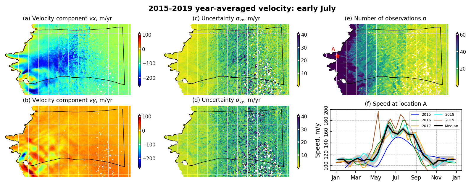
Figure 2Year-averaged velocity data set. (a–e) Horizontal surface velocity components (vx and vy), associated uncertainties ( and ), and number of observations per pixel (n). (f) Comparison between the original speed observations for the years 2015 to 2019 and the year-averaged data set where the grey shading represents the 1σ interval at point A in (e) and in Fig. 1. White pixels in maps (a, b, e) correspond to areas that are ice-free or with no data and in maps (c, d) to pixels with fewer than two velocity observations. The white grid lines are spaced by 10 km.
Besides the velocity maps, we generate a spatially distributed estimate of the velocity uncertainties for each temporal step. This uncertainty σ is computed per pixel as , where SD is the standard deviation of the averaged measurement in each time step and n is the number of averaged measurements. The typical range of n varies a lot in time and space (see Fig. 2e) due to the varying characteristics of the sensors and seasonal evolution of surface conditions (e.g. melting of snowfall). For instance close to the ice front it changes from few images in winter to more than 60 in summer. For the same reasons, the accuracy of the generated velocity maps varies over time and space. While for winter maps (January–April, December), the errors are generally below 10 m yr−1, these values can rise 3- to 4-fold between May and November, especially for the most inland areas where fewer observations are available and the smooth terrain makes satellite speed tracking difficult (see Figs. 2c, d and A1).
Our averaged data set is consistent with previous satellite products and ground observations in the area (Joughin et al., 2008; Palmer et al., 2011; Fitzpatrick et al., 2013; Lemos et al., 2018), as we observe the same range of speed and seasonal changes. The average winter speed varies from 50 m yr−1 outside of the main glacier trunks to 100–250 m yr−1 at Insunnguata Sermia and Russell Glacier and up to 300 m yr−1 at Ørkendalen Gletscher. At the end of spring and into summer, a pronounced speed-up is observed for the entire sector, with the acceleration starting at the ice margin and gradually moving upstream. As an extreme case, a short-term acceleration up to +360 % above MWS was observed over one small area (Palmer et al., 2011). However, the mean range of the speed acceleration spatially varies between +100 % and +250 % above MWS. Depending on the location, the deceleration starts in late June or July, continuing for 1 to 4 months. Consequently, the autumn velocity can be lower than the winter mean, which is especially typical for Ørkendalen Gletscher.
The ice in this sector flows in a clear east–west orientation with an averaged flow direction of about 275∘ from the north, except for Ørkendalen Gletscher. Therefore, the y-velocity component (vy) is close to zero (Fig. 2b), and variations in order of magnitude of several tens of metres per year can induce relatively large changes in the estimated flow direction. We noted in our time series that the flow direction varies up to ±25∘ across the year. This effect is only observed in velocity fields derived from the optical images and not in the synthetic aperture radar images, suggesting that this phenomenon is not related to a real change in ice flow direction. We attribute this effect to changes in surface illumination and shadow length being a function of solar elevation change from March to October and assume that it can induce the supplementary displacements of the surface feature footprints tracked by cross-correlation algorithms. Indeed, on Insunnguata Sermia, the mean vy velocity vector component changes from +60 to +10 and −40 m yr−1 between the velocity fields derived with Sentinel-2 optical images in early March (ascending low sun), late June (solstice), and early September (descending low sun) correspondingly. To deal with this phenomenon, we assume that the total magnitude of the majority of our time series was not severely affected. The most extreme case of the lowest sun angle and only optical imagery used with short time spans gives the magnitude overestimation by 10 % or about 10 m yr−1 for the average speed of 100 m yr−1 over the domain. So we only consider the norm of the velocity vector for the model inversions, keeping the vector direction to be defined by the model itself.
According to theoretical expectations, the ice flow is most likely to be affected by seasonal variations in surface runoff reaching the bed across the area that is under the equilibrium line. At Russell, the long-term equilibrium line is estimated to be at ∼1500 m (Van De Wal et al., 2012). Even so, the GPS records have shown the presence of a short summer speed-up further inland as well (Bartholomew et al., 2012; Greskowiak, 2014), with acceleration of about +5 % up to 50 km inland from the equilibrium line (Greskowiak, 2014). That corresponds to about +1 m yr−1 above the local MWS and is within the noise level in our velocity data set. For this reason the area of interest is limited to approximately 100 km upstream from the ice margin, which corresponds to a surface elevation of about 1400 m.
We use the finite-element ice flow model Elmer/Ice (Gagliardini et al., 2013) to compute the 3D velocity field in the Russell sector and infer the basal conditions over an entire “typical” year using the 24 surface velocity maps.
We use the basal topography given by BedMachine version 3 (Morlighem et al., 2017). The surface elevation comes from the Greenland Ice Mapping Project (GIMP; Howat et al., 2014), which has a nominal date of 2007. This is 10 years earlier than our velocity observations. Thickness changes in this area are about −1 m yr−1 near the margin (Helm et al., 2014; Csatho et al., 2014; Yang et al., 2019), which is relatively small compared to the ice thickness (see Fig. A2b); thereby we use it as it is. Over a single year the topography does not change significantly either. The average in situ observed rate is less than ±1 m yr−1 and partly attributed to the summer uplift by pressurized water (Bartholomew et al., 2010; Cowton et al., 2016). We therefore keep the surface topography fixed for all inversions. In doing so, we assume that basal changes are the only drivers of the seasonal ice speed variations and that changes in driving stresses due to surface elevation variations are negligible.
In the remainder of this section we describe the modelling domain, the model set-up, and the inverse modelling method.
3.1 Modelling domain and mesh
Our model domain corresponds to the ice catchment basin of the three land-terminating glaciers mentioned above, reaching to about 100 km inland for the reasons explained in Sect. 2 (Fig. 1). The lateral borders of the domain are defined by flow lines derived from the mean multi-annual observed surface velocity (Rignot and Mouginot, 2012). As the margin is land-terminating and thus does not require special boundary conditions at the front, the model domain has been extended a few kilometres in front of the margin in expectation of future transient simulations, leaving the possibility of an advance of the glaciers open.
To create the mesh, we start by meshing the horizontal footprint of the domain using the Elmer/Ice anisotropic mesh capabilities that rely on the MMG library (https://www.mmgtools.org/, last access: 20 February 2020; Dapogny et al., 2014). The mesh adaptation scheme equi-distributes the interpolation error of the observed surface velocities and thickness. Because the domain is relatively small, the mesh resolution is allowed to vary between 150 m near the margin and 400 m up to 40 km inland, with a maximum value of 1 km attained progressively beyond this. The resulting two-dimensional irregular mesh consists of approximately 60 000 linear triangular elements and approximately 30 000 nodes. It is then vertically extruded into 20 layers to form the 3D mesh. As the vertical velocity gradients are expected to be higher near the bed, the vertical resolution increases following a geometric progression and is 2 times smaller at the bed than at the surface. The 3D mesh is then stretched vertically so that the top and bottom surfaces follow the topographies given by GIMP and BedMachine. The model does not support meshes that have null thickness. In order to include ice-free areas, we therefore impose the arbitrary value of 0.9 m thickness for them. This thickness is sufficiently small that the remaining “ice” in the ice-free areas will have no impact on the results of the inversions and will avoid crashing the model.
Note that our study area is well-constrained by the radar measurements of ice thickness in the lower half of the domain, while the upper part of the basin has been much less surveyed (see Fig. A2a). A mass conservation algorithm (Morlighem et al., 2011) has been used for the interpolation of the basal topography in the densely surveyed area, while kriging is used outside (Morlighem et al., 2017). The latter is used when mass conservation is not practicable due to sparse thickness measurement and/or slow surface motion; thereby the resulting bed topography is often less accurate. Reported uncertainties in the bed elevation over the lower part of our domain, except the steep-slope front line, are generally lower than 30 m or below 6 % of ice thickness, while on the upper part they can reach up to 300 m, or 20 % of the ice thickness. We also notice that a few small-scale features are not well captured in the BedMachine version used here (v3.10, 20 September 2017), such as the southwestern nunataks next to Ørkendalen Gletscher that are actually ice-free but for which the data display an ice thickness of 100–140 m. The surface data provided by GIMP (Greenland Ice Mapping Project) are constructed from a combination of digital elevation models derived with ASTER and SPOT-5 satellites for the ice-sheet periphery and margin and photoclinometry derived with the AVHRR (Advanced Very-High-Resolution Radiometer) space-borne sensor in the ice-sheet interior (Scambos and Haran, 2002). Their uncertainty has been estimated by comparing with spaceborne lidar altimetry from ICESat satellites and is about ±1 m over most areas of interest (Howat et al., 2014).
3.2 Direct model
3.2.1 Field equations
To compute the 3D ice velocity (u) and ice pressure (pi) fields, we solve the Stokes equations that express the conservation of momentum and mass for an incompressible fluid:
where ρ is the ice density, g is the gravity vector, and is the Cauchy stress tensor with τ the deviatoric stress tensor and I the identity matrix.
To close the system, we use the classical viscous isotropic power law, known as Glen's flow law, that non-linearly relates the deviatoric stress tensor to the strain rate tensor as
where the effective ice viscosity η is given by
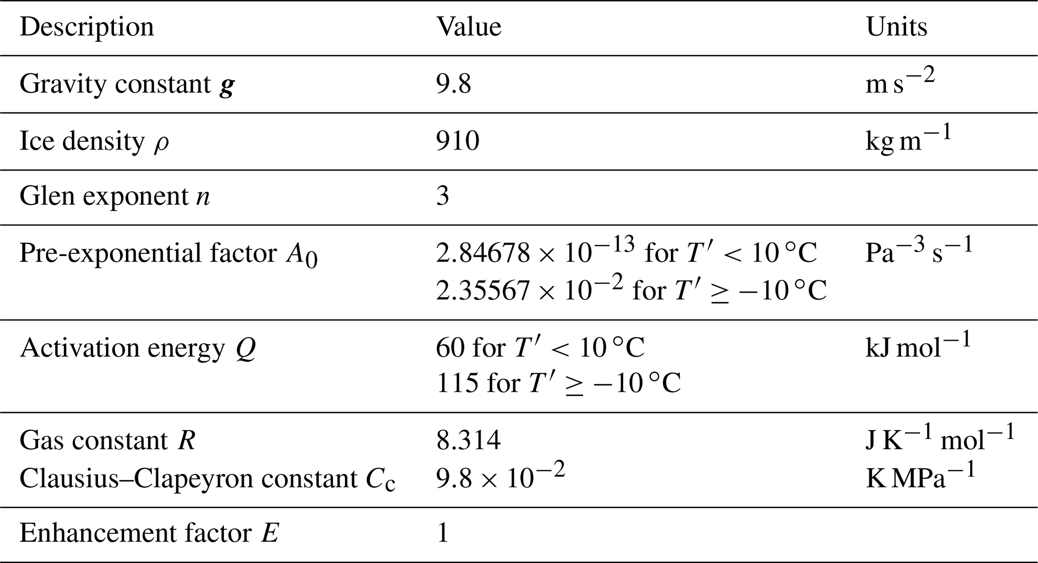
where the second invariant of the strain rate tensor is given by , n is the Glen exponent, and E is an enhancement factor, and the rate factor A depends on the ice temperature T following an Arrhenius relationship:
where A0 is the pre-exponential factor, Q is an activation energy, R is the gas constant, and , where the pressure melting point is given by with Cc the Clausius–Clapeyron constant. The parameter values used by us are given in Table 1.
Initializing the temperature field is a difficult problem as the thermal state in an ice sheet has a long-term memory requiring multi-millennial spin-up simulations (Goelzer et al., 2017), and the heat sources are in general poorly constrained and make the thermo-mechanical problem non-linear (Schäfer et al., 2014). Here we use the temperature field simulated by the ice-sheet model (http://www.sicopolis.net/, last access: 18 June 2019) for the present state of the Greenland ice sheet (Goelzer et al., 2020).
We have compared the temperature profiles to existing in situ borehole measurements from the ablation zones of Insunnguata Sermia (Harrington et al., 2015; Hills et al., 2017). Results are shown in Fig. A3. The modelled temperature appears to fit the observations better at higher altitudes around 40 km from the ice margin (Hills et al., 2017; Harrington et al., 2015, location S5) than at lower altitudes (Harrington et al., 2015, locations S2–S4). This is likely because SICOPOLIS does not have the resolution and processes to accurately capture the individual land-terminating glaciers. Within the first 40 km from the glacier terminus, observed temperatures are generally warmer than −6 ∘C across the entire ice column, while the model finds the temperature to be up to 6 ∘C cooler across the ice column. Further inland from the glacier terminus, both measurement campaigns found that the temperature decreases from −10∘ at the surface to −13 ∘C at a depth of about 200–300 m and then rises to near-melting temperature at the glacier base. Here the SICOPOLIS temperature follows a similar trend with a slight 1–2 ∘C warmer divergence over the ice column but becomes cooler about 200 m above the bedrock. At the glacier base, the model shows in all boreholes a deviation of 2–4 ∘C below the measurement, meaning that the measured temperature at the base is closer to the melting point than SICOPOLIS estimates. As deformation rates increase rapidly and non-linearly with increasing ice temperature (Eq. 4), the generally colder modelled ice could potentially cause the ice flow model to underestimate the internal deformation compared to reality. However, the investigation of the influence of temperature field uncertainties on the basal-friction inversions shows a more limited influence than, for instance, uncertainties in the basal topography (Habermann et al., 2017). As the temperature field reproduces part of the observed spatial variability sufficiently well, in the following, we briefly assess the sensitivity of the results to the ice rheology only by changing the value of the enhancement factor E. To validate the final rheology parameterization, the model-derived ice deformation profiles are compared further against in situ borehole measurements (Sect. 4.3).
3.2.2 Boundary condition
As we model only a part of the ice sheet, in addition to the conditions at the top and bottom surfaces we have to prescribe boundary conditions at the sides of the domain. Note that the lateral sides of the domain have been chosen to be sufficiently far from the regions of interest so that, for the diagnostic simulations presented here, the details of the boundary conditions should not affect the solution at distances greater than a few ice thicknesses. For all the boundaries, we denote by n the unit vector normal to the boundary and pointing outward from the model domain.
The lateral sides of the domain coincide with flow lines so there should be no ice flux entering the domain. We therefore impose the following condition:
Along the tangential directions, we keep the natural stress-free condition and thus neglect the tangential shearing components along these boundaries. At the inflow boundary (Γi) we apply Dirichlet conditions for the horizontal components of the velocity vector () using the observed surface winter-mean velocities () (see Sect. 2):
Note that we impose uniform velocities along the vertical direction and thus neglect the deformation profile at the starting point of the initialization model run. The deformation of the ice column occurring in the inland areas of the modelling domain are the modelled state adapted to the given boundary conditions. We expect that the results a few ice thicknesses from the border should be insensitive to the prescribed non-deforming vertical profile at the lateral borders (Mangeney et al., 1996; Gagliardini and Meyssonnier, 2002). This is consistent with observations in the area (Maier et al., 2019) and with our model results (Sect. 4.3), which show that the deformation profiles contribute to only a small portion of the surface velocities. We leave the natural stress-free condition for the vertical direction and thus neglect vertical shearing along this boundary.
The bottom and top surfaces correspond to natural interfaces of the ice. For the upper surface, Γs, we neglect the atmospheric pressure and impose a stress-free condition:
For the bottom boundary, Γb, we use a linear friction law that relates the tangential basal shear stress, , to the basal sliding velocity and a no-penetration condition for the normal velocity:
where is the tangential operator, and β is an effective friction coefficient which is tuned using the inverse procedure described in the following section. Hereafter, we will mainly refer to the norm of the sliding velocity and basal friction denoted by and .
The results of the inversions using a fixed geometry and a single velocity data set have been shown to be weakly sensitive to choice of friction law as the friction field must satisfy the global stress balance (Joughin et al., 2004). This has been confirmed in the area by Koziol and Arnold (2017), who found very small differences when comparing the basal shear stress fields inverted using three different friction laws.
3.3 Inverse model
Inverting for the basal friction coefficient using the observed surface velocities is now widespread in many ice-sheet models (Jay-Allemand et al., 2011; Gillet-Chaulet et al., 2012; Larour et al., 2014; Shapero et al., 2016; Maier et al., 2021a). Here, we use the variational control inverse method implemented in Elmer/Ice (Gagliardini et al., 2013), and in the following we highlight the main steps.
For a given observed surface velocity field, the optimal effective basal friction field β in Eq. (8) is found by minimizing the following cost function:
where J0 is an error term that measures the mismatch between model and observed surface velocities and Jreg is a regularization term weighted by the regularization parameter λ. As the effective friction coefficient must remain positive, we use the following change of variable β=10α, and the optimization is done on α.
We define J0 as
where is the norm of the model horizontal surface velocity vector interpolated at the Nobs locations where we have an observation for the horizontal surface velocity (the nodes of the storage file grid, in fact), with σu the norm of the vector composed by the estimated velocity uncertainties (see Sect. 2). Note that here we have chosen to compare only the norm of the vector and disregard the error on the flow direction, as the direction is mainly governed by the topography and, additionally, may be biased in our velocity observations, as explained in Sect. 2.
To regularize the inverse problem, Jreg is a Tikhonov regularization term that penalizes the horizontal derivatives of α as
The gradients of Jtot with respect to the nodal values of α are computed by using the adjoint model, and the cost function is minimized using the limited-memory quasi-Newton routine M1QN3 (Gilbert and Lemaréchal, 1989).

Figure 3(a) Modelled horizontal surface speed, (b) basal sliding speed, and (c) basal friction inferred from the mean winter surface speed (MWS) overlaid on the basal topography hillshade. Panel (d) shows the difference between modelled and observed surface speed. The white grid lines are spaced by 10 km.
4.1 Mean winter state
4.1.1 Model set-up
We start with an inversion of the MWS velocity map to get the initialization state for our seasonal investigations. The friction coefficient is initialized using a previous inversion performed with Elmer/Ice for the whole Greenland ice sheet using the shallow-shelf equations for the force balance, and the minimization is stopped after 200 evaluations of the cost function. Based on such procedure, we run six inversions for different values of the regularization parameter λ. Following the L-curve method (Hansen, 2001), the optimal parameter is a compromise between fitting the observations and having a smooth solution which should correspond to the point of highest curvature in a log–log plot of the regularization term against the error term. We plot those L-curves and report the mean relative error in Fig. A5a. The curves show the expected behaviour where increases as λ and Jreg decreases. In the absence of model errors and for uncertainties accurately estimated and normally distributed, we should expect to be close to 1. Here, for the smallest regularization we obtain a minimum . For the following seasonal investigations, we choose the value λ=2500, which gives a relative error just above 1 and is located in the area of highest curvature. Additionally, we observe that the results are weakly sensitive to the exact choice of λ as the standard deviation of the sliding speed and basal friction computed over all tested values of λ, except the smallest and the largest ones are generally below 5 % in 92 % and 91 % of nodes respectively.
4.1.2 Results
The modelled surface speed, sliding speed, and basal friction for the mean winter state are shown in Fig. 3. The modelled surface velocity shows a good agreement with the observations (Fig. 3d), with a root-mean-square error of about 3 m yr−1, similar to the reported uncertainties (Fig. A5b). We notice however large differences (up to 30 m yr−1) between the modelled and observed velocity for a few places. This is especially true near Ørkendalen Gletscher where some nunataks are not correctly represented in BedMachine. A similar issue with under-resolved subglacial features may also explain the speed mismatch on the other side of the Ørkendalen valley where BedMachine shows a large uncertainty (>140 m). These areas appear with a particularly high friction compared to the rest of the domain (>0.2 MPa) and nearly no sliding, meaning that the velocities resulting from vertical shear are already larger than the observations, likely because of the overestimated ice thicknesses. The areas of friction close to zero along the margin could be due to underestimation induced by BedMachine as well, as here, on the steep slopes of thin ice, the reported error-to-thickness ratio is larger than 50 % (Fig. A2a).
The spatial pattern of the basal velocity is very similar to that of the surface. We obtain a sliding ratio of about 0.9 for most of the domain, consistent with deformation profiles measured in the area (Maier et al., 2019). Deformation-induced speed estimated as is generally on the order of 10–15 m yr−1 and can locally increase to up to 30–50 m yr−1 in locations of high traction.
For most of the domain, the inferred basal friction τb is on the order of 0.1 MPa. These values are consistent with previous inversions in the same area performed by Koziol and Arnold (2017) using winter 2008–2009 velocities. Together with a typical sliding velocity of 100 m yr−1, this falls in the velocity–traction relationship derived at the catchment scale by Maier et al. (2021a), which was interpreted as indicative of hard-bed conditions. However, Maier et al. (2021a) also found several patches in this catchment where the bed is weaker than the average. We also observe a few areas where relatively high sliding speeds correlate with particularly low friction compared to elsewhere, with values lower than 0.05 MPa. This is particularly true for a large fraction of Ørkendalen Gletscher, but can also be seen at the tongue of Russell Glacier. While for the glacier terminus we cannot rule out an under-estimation of the ice thickness that would be compensated for by higher inferred sliding speed, this would also be consistent with a “weak” bed offering less resistance due to the presence of deformable till or substantial cavitation. To our knowledge, no in situ measurements have been done on Ørkendalen Gletscher to confirm the presence of till, but seismic measurements suggest the presence of subglacial sediment within 13 km of the terminus of Russell Glacier (Dow et al., 2013), in agreement with the weak bed assumed by us.
There is no such low friction under Insunnguata Sermia, where the flow is well constrained by a subglacial valley for the first 25 km inland from the terminus. This is in agreement with Harper et al. (2017), who found no evidence of soft sediments at the bed of Isunnguata Sermia from their network of 32 boreholes. However, no borehole reached the bottom of the valley, where the friction is locally the lowest, it being higher on the adjacent sides. Higher upstream, the subglacial valleys are not aligned with the ice flow lines, and, in general, we have higher friction on the leeward sides of the valleys. The spatial heterogeneity of the basal friction shows that it is possible to reconcile opposite views on the nature of the bed in this sector (Booth et al., 2012; Dow et al., 2013; Kulessa et al., 2017; Harper et al., 2017), as the basal conditions of this sector are heterogeneous and can likely change from an inferred hard to weak bed over distances of a few ice thicknesses. Additionally, this could suggest that some specific conditions are required for till accumulation, for instance topographic depressions or lack of drainage efficiency, forming the non-uniform bed properties in the long run.
4.2 Seasonal inversions
4.2.1 Model set-up
To investigate the year-around behaviour of the basal friction and velocity fields, we perform the inversions for each of 24 velocity maps presented in Sect. 2 (hereafter called “time steps”) in a similar way as described above for MWS.
As the observation errors are not uniform in time, to assess the sensitivity of the summer results to the regularization, we run a new L-curve analysis with the early July velocity data set. The results are shown in supplementary Fig. A5a. The minimal value of is now close to 2. This could be due either to an under-estimation of the uncertainties on observed ice speed for these 2 weeks or to the model not being able to exactly match the summer observations. The latter could be due to model errors not taken into account or because reducing the observations to a standard year leads to more inconsistencies in summer as there is more variability during this period compared to winter. In addition, we found that the results are more sensitive to the choice of λ than for the MWS inversion, as the standard deviation on ub and τb between the different tested λ, except the smallest and the biggest one, is about 15 %. However, we remark that the dependency of Jreg on λ is relatively similar to those obtained with the MWS data sets, and the value λ=2500 seems consequently to also be a good compromise for this early July data set. Thereby, this λ value is used for inversions of all 24 time steps.
To reduce the computational burden for the independent twice-monthly inversions, the basal friction coefficient field is initialized each time using the solution obtained for MWS inversion. As we cannot guarantee in general that the given λ will be optimal for all the data sets, we stop the minimization after 30 evaluations of the cost function to avoid overfitting. This choice is motivated by the fact that in general the cost function decreases rapidly during the first iterations and then stagnates at a value close to the noise level where it may overfit the observations if regularization is not used (Arthern and Gudmundsson, 2010; Habermann et al., 2012). This can be clearly seen in Fig. A5b for the spring and summer months, where the error decreases during the first 10 to 20 iterations then stagnates. Note that the error can locally increase between two successive evaluations of the cost function, as the global convergence is enforced by a line-search phase so that the minimization routine effectively checks that the cost function decreases globally. As expected, because the velocities are relatively stable during the winter months and thus close to the MWS, the error is already very low when compared with the initial guess and stabilizes or eventually slightly increases (while Jreg decreases) during the iterations.
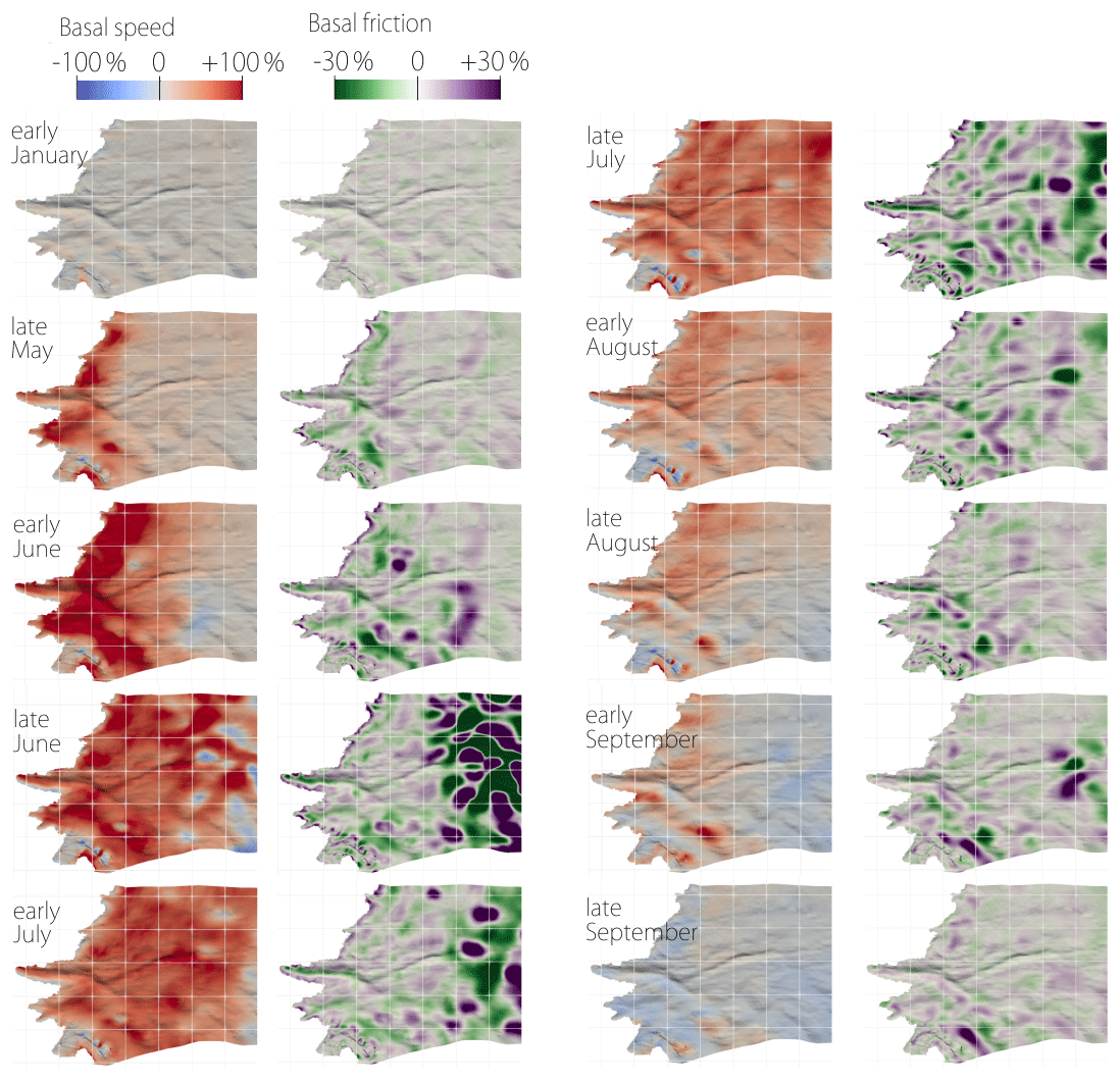
Figure 4Seasonal change of basal sliding speed (left subcolumns) and basal friction (right subcolumns) relative to the winter mean state, with basal topography hillshade added. The white grid has a 10 km step.
In Fig. A1, we show the misfit maps as the difference between observed and modelled surface ice speeds (only for the early half of the months as the second halves usually show a similar range of mismatch). The periods showing the largest misfit correspond to the transition between different surface conditions. This is especially true in June, July, and September, when the surface changes from snow-covered to melting ice or vice versa. Note that the November data set seems more likely to be corrupted by poor satellite imagery than by the surface conditions. The uncertainty in the observed velocity for these periods often exceeds 30 m yr−1, which represents a significant relative uncertainty in the upper part of the domain where speed is below 100 m yr−1. However, the surface velocity is captured relatively accurately in the first 50–70 km from the margin, and the inversions give a good match between the adjacent time steps, giving us confidence in the interpretation of the basal fields in these areas. Taking that into account, as well as the uncertainties in basal topography, we mainly discuss the results on the downstream half of the modelling domain.
4.2.2 Results
In Fig. 4, we present the ratio of the inverted basal friction τb and sliding speed ub for 10 inversions (out of the 24) to their winter mean state. Results from early October to early March are fairly similar, so we show only early January as an example of this period. From late March to late September, the relative changes in τb and ub are shown every 2 weeks. Note that the extreme τb variability in late June and early July over the upper shown area is most likely unrealistic and induced by the discussed quality of the input surface velocity fields.
These inversions demonstrate that ub doubles first along the ice margin, and then the acceleration propagates inland until mid-July. Thus, in the first 20 km from the ice margin, the maximum sliding speed is reached by early June, whereas higher up the peak it only arrives later in early July. Similarly, the sliding speed first decreases along the ice margin and then the deceleration propagates inland until the end of September. In late September, the velocity is generally lower than the MWS by about 10 % to 20 % in the first 10–15 km from the margin, while it is still slightly higher or equal further upstream.
Following changes in sliding speed, the basal friction τb first decreases along the ice margin in late May. Over time, this decrease then propagates higher up inland, mainly in subglacial valleys and depressions. Note that the lowering of τb is usually correlated with the highest increases in sliding speed. However, as the global force balance must be maintained, this decline cannot be widespread. Thus, the stresses are redistributed locally and simultaneously on higher parts of the bed or on the sides of subglacial valleys where the friction rises. The sliding speed here rises as well, but it is less pronounced. Both increases and decreases in τb over the domain are of the order of ±30 %. By late September, τb returns to its winter state. One exception is Ørkendalen Gletscher where it remains higher and where we also have the most significant decrease in sliding speed in autumn compared to the mean winter value.
4.3 Ice deformation versus sliding speed
An interesting question is how the contributions of deformation and sliding to the surface speed change seasonally. Ice viscosity and surface topography are fixed in inversion set-ups; therefore the temporal variability in the ice deformation rate occurs only due to the change in the inferred basal friction (thus, in the shear stress). We found that in summer, on average across the domain, the magnitude of the deformation speed ud increases, but the proportion of surface velocity it represents decreases. The mean winter value of ud across the domain is about 8 m yr−1, rising to about 20–30 m yr−1 in some topographically predefined locations (Fig. A4a). In early July it rises by +12 % above winter on average (Fig. A4b). At the same time, the contribution of deformation to glacier surface motion estimated as a fraction slightly decreases from winter to summer over the majority of the domain (see Fig. A4c), with mean values of 10 % and 8 % respectively and an absolute change rate of a few metres per year. That means the sliding velocity represents about 90 % of the surface flow in winter and slightly more when velocities increase in summer. As expected, the summer acceleration observed on the surface is mainly due to enhanced sliding. In a full-Stokes model, the entire 3D velocity field depends on the material properties and boundary conditions, so that the deformation profiles are not constant in time. Here only model-inferred basal friction can influence the deformation profile, making it variable from one inversion to another. If the deformation changes remain small compared to changes in sliding velocities in magnitude (Fig. 5a), it is interesting to note that, by changing only the basal conditions in the model, the relative changes in deformation rate are important between winter and summer. Similar in situ observations have been made by Maier et al. (2021b) by examining spatio-temporal changes in deformation, sliding, and surface velocities over a 2-year period using GPS and a dense network of inclinometers installed in borehole grid drilled in Ørkendalen Gletscher.
Although direct measurements of sliding velocities and ice deformation rates are rare in Greenland, Maier et al. (2019) estimated them within a network of boreholes located approximately 20 km from the ice margin of the Insunnguata Sermia catchment (blue star in Fig. 1). These observations were made during the winter season 2015–2016 in boreholes spaced by about 150 m and include GPS (providing the surface velocity), temperature, and inclinometry (providing the deformation). At this site, the deformation was found to account for only 4 % of the surface velocities, and, thus, ice sliding was responsible for the overwhelming majority of surface velocity during the winter. In addition, their measurements show that the majority of deformation happens in the first 150 m above the bed and that almost no deformation occurs in the upper 75 % of the ice column.
We compare the measurements made by Maier et al. (2019) with the modelled fields at the same location in Fig. 5a and b, in the form of vertical profiles of the horizontal velocity magnitude and shearing rates . The inverted sliding and surface velocities in winter of about 105 and 115 m yr−1 are in agreement with the in situ measurements of 110 and 114 m yr−1 respectively. It would appear that the model produces a slightly larger deformation speed ud than observed (10 m yr−1 versus 4.6 m yr−1 in the in situ observations), with excess deformation mostly coming from the upper 75 % of the ice column and thus not expected to vary in time with changes in basal friction τb.
During the velocity peak in early July, the deformation speed ud in our inversions rises up to 15 m yr−1 and thus increases relative to winter by about +50 % (maximum ud is 19 m yr−1 in early August or +90 % from winter, Fig. 5a). At the same time, basal sliding speed ub increases from 105 to 165 m yr−1 (+57 %), and surface speed us increases from 115 to 180 m yr−1 (+57 %). Consequently, at this specific point, the relative increase in surface flow velocities from winter to summer is about 8 % due to an increase in the deformation rate, and the remaining 92 % corresponds to the accelerated sliding. Note that the overall contribution of ud to the surface speed is almost invariable from winter (9 %), being slightly lower at the moment of maximum glacier motion (8 %) and slightly higher when deformation of basal layers intensifies (10 %).
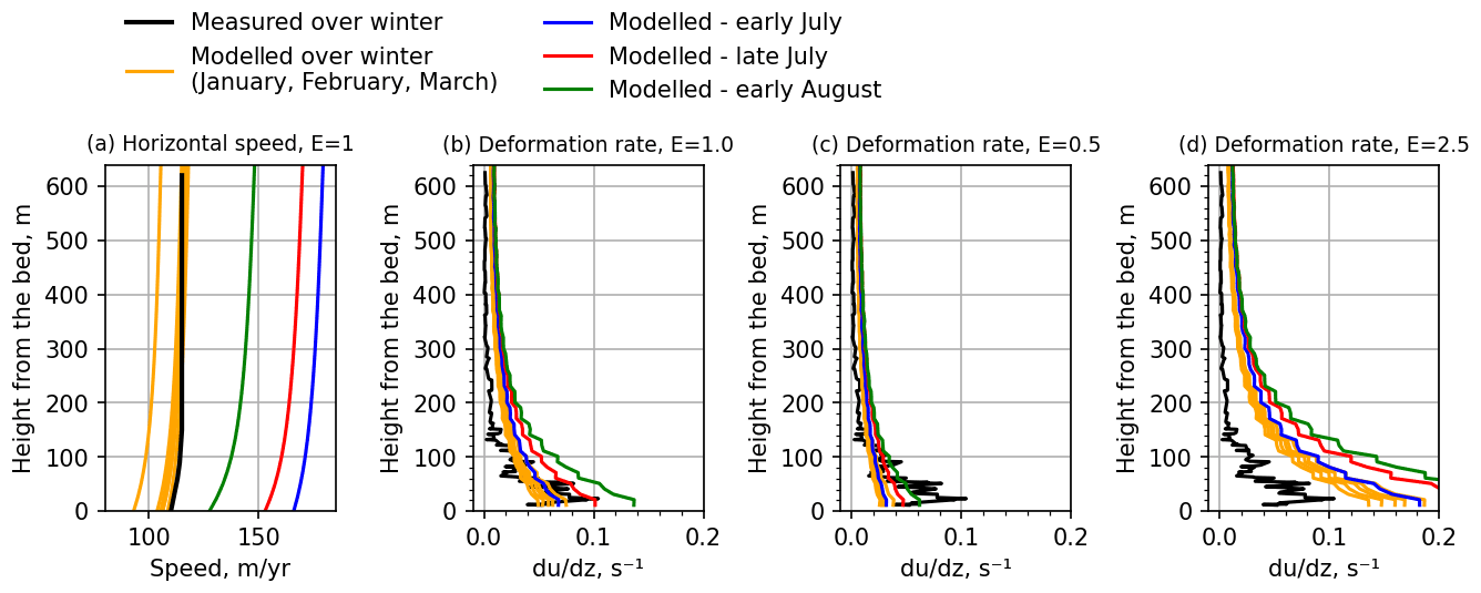
Figure 5Vertical profiles of modelled (a) horizontal velocity magnitude and (b–d) vertical shear rate for varying enhancement factors E at the location of borehole measurements done by Maier et al. (2019), drawn here in black.
It should also be noted that the actual magnitude of modelled deformation and sliding velocity in this analysis depends on the constitutive law used for the ice rheology (here, Glen's flow law, Eq. 2). In this study, we assume a viscosity enhancement factor E=1 (see Eq. 3) to describe the ability of ice to deform. This means we adopt Glen's rheology parameters constrained via laboratory experiments without any modifications. Larger values of E would correspond to simulation of softer ice, while lower values of E represent stiffer ice, which provides the adjustment of viscosity imposed by laboratory parameters if required. In Fig. 5, we test different values of E against in situ observations from Maier et al. (2019) by comparing the vertical deformation rate obtained for inversions performed with E=0.5, 1, and 2.5 with the mean measured winter deformation profile obtained over nine boreholes.
With E=0.5, and thus stiffer ice, the model reproduces the winter deformation rate well over most of the ice column but underestimates it for the lower 100 m above the bedrock; there the majority of shearing happens according to observations. In this case, even with enhanced shearing in summer, modelled deformation does not reach the level observed in winter. With E=2.5, the ice deformation is much larger over the entire ice column than observed, suggesting that the modelled ice is too soft. A value of E=1 provides a good compromise where the deformation rate over the winter months near the bed is similar to that of the in situ measurements and does not deviate significantly at other depths.
4.4 Relation between τb and ub
To further discuss the leading processes behind the seasonal variability of basal fields, we take a closer look at three different locations that are representative of the main types of τb-versus-ub behaviour obtained across the modelled domain (Fig. 6). As the aim will be to interpret the results in terms of friction law, we show the seasonal evolution of τb as a function of ub (bottom subplots) together with their evolution during the year (top subplots).
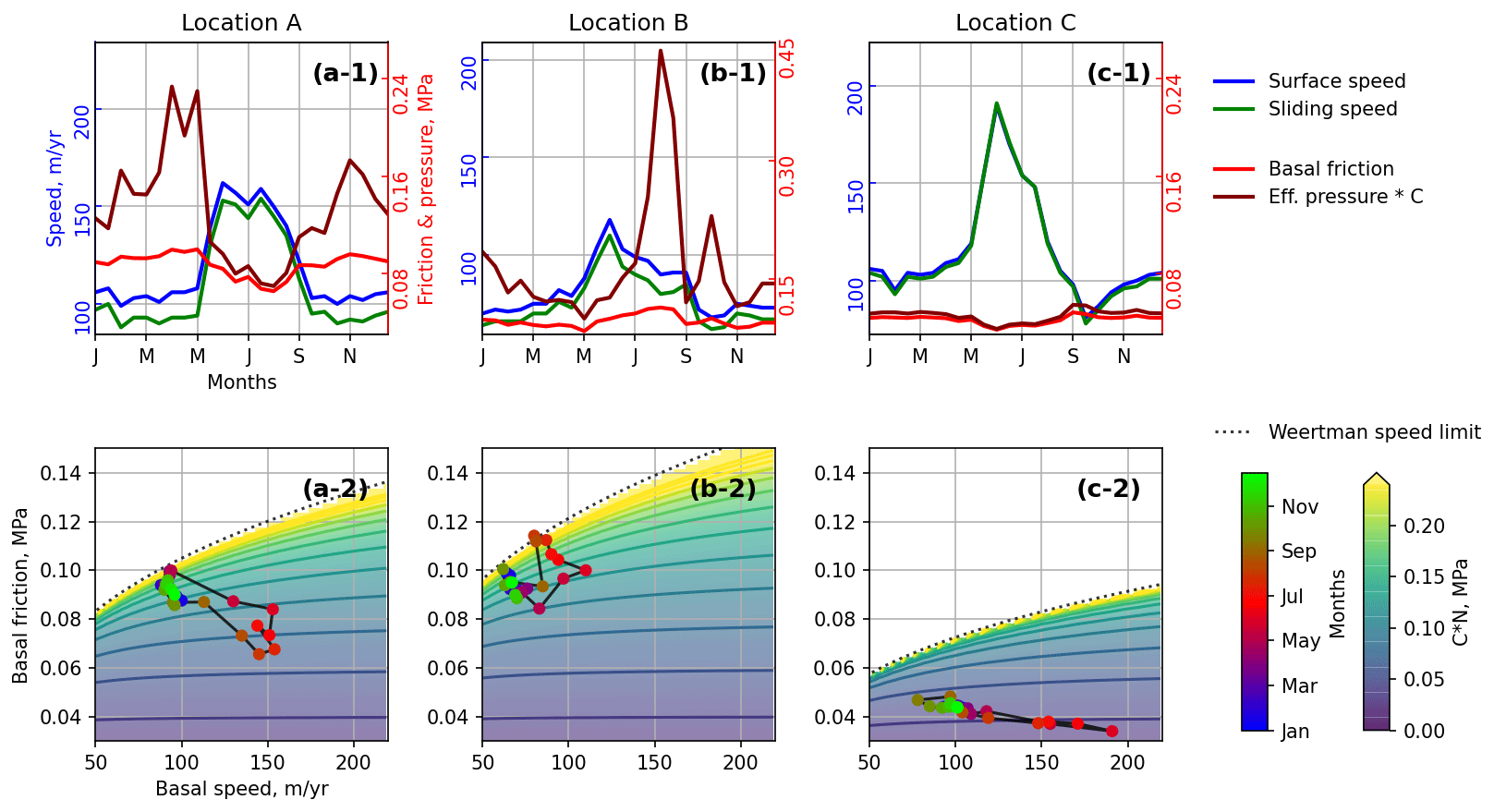
Figure 6Surface speed us, sliding speed ub, basal friction τb, and scaled effective pressure CN at three locations indicated in Fig. 1. (a-1–c-1) show the evolution of us, ub, τb, and CN as a function of time. Panels (a-2–c-2) represent the evolution of the relation between τb and ub throughout the year, where the coloured background shows the scaled effective pressure CN obtained from Eq. (12) with the solid lines corresponding to isovalues spaced by 0.02 MPa. The dotted line represents the upper limit corresponding to the Weertman regime (see Sect. 5.1).
In the first case, at point A located at the Insunnguata valley floor about 10 km from the ice margin (see Fig. 1), we have a clear anti-correlation between friction and sliding speed. The friction slightly rises from January to May, but there is no clear trend for the velocity. Notable acceleration starts in early May in conjunction with a decrease in τb. High sliding velocities, 65 % above the winter average, are maintained until mid-July with some variability. At the same time, the basal friction continuously decreases until August, with a minimum at 30 % below the winter average. After that, ub decreases and τb increases back to winter values. The seasonal evolution of τb as a function of ub shows a clear hysteresis where for the same friction, the sliding speed is higher during the acceleration phase (spring) than during the deceleration phase (autumn). Such an effect, interpreted as an opening–closing of the subglacial water cavity and/or longitudinal stress coupling with the upper parts of the glacier, was already observed in situ (Sugiyama and Gudmundsson, 2004) and studied numerically (Iken, 1981). In our results, the regions that experience this type of behaviour are mainly the subglacial valley bottoms where the basal friction is not too low in winter (∼0.1 MPa).
Point B is positioned on the northern valley slope of Insunnguata Sermia at about the same distance from the ice margin as point A. Here, during the warm season, the basal friction globally rises (+20 %) together with basal sliding (+80 %). However, there is a preceding phase from January to May where the sliding speed slightly increases in conjunction with decreasing friction. The clear acceleration in May correlates with an increase in friction. Further, the sliding velocity starts to diminish in June while the friction reaches its maximum only in August. This relation between τb and ub is generally associated with valley sides and higher basal topography.
Point C is located at Ørkendalen Gletscher about 10 km along the glacier flow line from the ice margin (Fig. 1). This point is typical of areas with lower-than-average friction values (<0.05 MPa); i.e. the base offers little resistance throughout the entire year. Here, the velocity increases almost 2-fold from late April to late May and is associated with a relatively small absolute change in friction of about 0.01 MPa compared to point A where τb dropped by almost 0.04 MPa. For this point, it is also worth noting that the speed minimum appears in early September, clearly below the winter mean. As for point A, changes are mostly anti-correlated; i.e. sliding rises with decreasing friction and vice versa, and the maximum in ub corresponds to a minimum in τb.
5.1 Water-dependent friction law
5.1.1 Definition of the friction law
To interpret the variations in the basal friction and velocity in terms of water pressure, we adopt a friction law that has been originally proposed to represent the flow of clean ice over a rough bedrock with cavitation (Schoof, 2005; Gagliardini et al., 2007). In its simplest form, this friction law relates the basal friction τb to the effective pressure N and the sliding velocity ub and, following Gagliardini et al. (2007), is expressed as
where As is the sliding parameter without cavities, C is a parameter related to the maximum bed slope, and the exponent n is usually equal to the flow law exponent in Eq. (2). The effective pressure N conceptually represents how frictional forces are reduced by the presence of pressurized water and is equal to the difference between the Cauchy compressive normal stress to the bed surface and the water pressure pw. Here we approximate the normal stress by the ice pressure pi solution of the Stokes system; thus . In practice, pi is close to the hydrostatic ice overburden pressure pi≈ρgH, and this allows it to be consistent with observations of the water pressure that are reported as a fraction of the ice overburden pressure. A friction law of a type similar to Eq. (12) has been used by several ice flow models coupled with a subglacial hydrology model (Pimentel et al., 2010; Hewitt, 2013; Gagliardini and Werder, 2018; Cook et al., 2021). While Eq. (12) was primarily developed for hard beds, a similar expression has been proposed for deformable beds by Zoet and Iverson (2020). The main difference is that for a given basal friction, their expression predicts that ub tends to zero at high effective pressure while it tends to the Weertman sliding velocity with Eq. (12). Similarly to account for the two friction regimes, a regularized Coulomb friction law where the dependency on N is not explicit but parameterized has been proposed by Joughin et al. (2019) and has been shown to provide a good fit to observations for Pine Island Glacier, Antarctica. Some authors (Koziol and Arnold, 2018, 2017; Brinkerhoff et al., 2021) have used a different friction law where the dependency on N has been introduced in a mostly empirical manner (Budd et al., 1979). While Koziol and Arnold (2018) found that this last law gives a slightly better fit to observations than Eq. (12) in a coupled ice flow–hydrology model of a glacier, we do not consider this law as it has less physical background and does not satisfy Iken's bound (Iken, 1981).
Designing our workflow, we preferred to invert for the effective friction coefficient (β in Eq. 8) first and then interpret its temporal variations in terms of effective pressure in a second step. There are several reasons for this. First, it should be numerically more stable to use a linear relation in the numerical model. In winter, including the MWS case, the friction law involving the effective pressure is close to the Weertman regime and thus weakly sensitive to N, meaning that the modelling results would be much more sensitive to the regularization process described in Sect. 3.3. Second, this two-step approach allows us to carefully address the choices of As and C parameters of the effective pressure-based law.
From Eq. (12) it can be shown that the product CN can be expressed as a function of the fields τb and ub, which are solutions of the inverse problem, and the parameter As as
Expressed this way, it is easy to see that this expression exhibits two asymptotic behaviours.
-
When , the relation tends to a Coulomb-type friction law τb=CN, and the effective pressure does not depend on the sliding speed ub anymore. That implies a lower bound for Eq. (13) N>0, so we cannot get a water pressure exceeding the ice pressure. However, even if that is observed with local in situ measurements (Wright et al., 2016; Hoffman et al., 2016), the water pressure greatly exceeding ice overburden is very unlikely (Doyle et al., 2015). Thereby both very small positive and negative N values practically lead to the same outcome of near-zero friction in the model.
-
When , CN→∞, and at the limit the basal friction is described by the classical Weertman friction law . In practice N should satisfy the upper bound N≤pi, meaning that the water pressure must remain positive.
Finally, the case is incompatible with Eq. (13) and means that the inverted values are inconsistent with the choice of As as the bed is already too slippery even without water.
5.1.2 Choice of the sliding parameter As
The sliding parameter As should depend on the near-basal ice rheology and on the small-scale roughness of the bed and thus is likely to be variable in space. Large values of As correspond to a slippery bed even without water, while low values represent a bed that offers more frictional resistance to the flow. Thus, depending on the choice of As, one can approach the Weertman or Coulomb limits of the friction law defined in Eq. (12). This will obviously affect the effective pressure values N retrieved but also the amplitude of the seasonal changes expected to be observed.
Using a similar method to infer changes in water pressure from several inversions of the basal conditions under Variegated Glacier over a year, Jay-Allemand et al. (2011) compute a spatially varying As so that the upper bound N≤pi is always fulfilled. In an application to the same area we investigate, Koziol and Arnold (2017) use winter velocities and a modelled winter basal water pressure field to invert for a single parameter in a friction law similar to Eq. (12). Their coefficient μb corresponds to our C, and they use a constant value for the product AsCn (i.e. their λbAb), so that for us this would correspond to spatially varying As and C. They found that the whole domain is close to the Weertman regime in winter.
Here, to spatially constrain As, we first compute the sliding coefficient that would be obtained in the Weertman regime using ub and τb from the MWS inversion. The derived coefficient corresponds to an “effective” as it will reflect the effective winter state of the bed roughness which could include the smoothing effects of potentially existing cavities that are not closed or kept open by basal meltwater (Cook et al., 2020).
The distribution of at the mesh nodes is shown in Fig. 7a. The median value is m Pa−3 s−1, corresponding approximately to a basal traction τb of 0.1 MPa for a sliding speed of about 100 m yr−1. The same order of magnitude is found by looking at the relations between τb and ub inferred by Maier et al. (2021a) at the scale of the GrIS catchments that are identified as being subject to hard-bed physics (see authors' Supplement, Fig. S9 and Table S1). Our estimate also has a consistent order of magnitude with the value used by Hewitt (2013) and Gagliardini and Werder (2018) in synthetic applications developed to represent a typical Greenlandic land-terminating glacier such as those in the Russell sector.
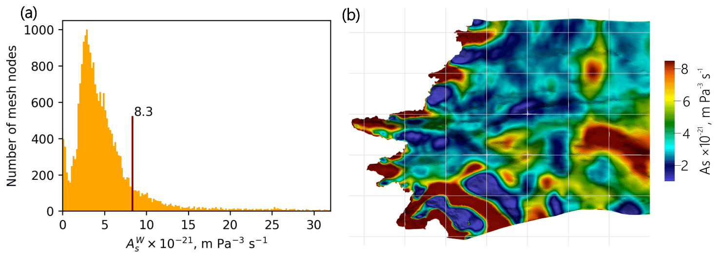
Figure 7(a) Histogram of . (b) Map of the As derived with Eq. (15) and used for water pressure calculation, with basal topography hillshade added. The white grid lines are spaced by 10 km.
The spatial distribution of mostly reflects the inferred winter basal friction (Fig.3c), where the areas with low friction would imply a very slippery bed. As mentioned previously, if we assume that these areas of weak bed might be underlain by deformable till or too many water-filled cavities maintained over the winter, the value of has no meaning in its Weertman law sense, and these areas should be described with a Coulomb friction law. It is then reasonable to impose an upper bound for As. There is no obvious upper limit, and we arbitrarily choose m Pa−3 s−1 (Fig. 7a). That limit covers 85 % of the mesh nodes and puts the areas of very likely assumed weak bed (Ørkendalen Gletscher valley, Russell Glacier tongue) in the Coulomb regime while leaving the areas of strong bed in the Weertman one.
Directly taking to compute N from Eq. (13) would lead to incompatibilities for some nodes in some inversions, i.e. . We therefore choose to lower As as , where is the uncertainty on estimated by uncertainty propagation of inferred ub and τb computed as
where and are the standard deviation of the basal speed and friction obtained from the six inversions of the winter months from January to March, as we assume no significant changes in basal conditions over this period. Our winter velocity and friction uncertainties are about 4 % and 2 % respectively on median across the domain.
As more than 90 % of nodes have the January to March variability of τb and ub values under ±2δ from mean winter state, we consider it sufficient to use to avoid upper bound incompatibility of Eq. (13) (see Sect. 5.1.1) across the majority of the area. Therefore, As is taken as
which brings together the initial slipperiness assumed under Weertman conditions, scaled down with respect to uncertainties in modelled basal velocity and friction and the arbitrary prescribed boundary to deal with weak-bed regions. Figure 7b represents the final field of As used further to infer water pressure, with maroon areas corresponding to the weak-bed regions restricted by .
Reducing As compared to is also consistent with observations in boreholes that suggest locations of relatively high water pressures pw, above 80 % of the overburden pressure pi, even in winter (Van De Wal et al., 2015; Wright et al., 2016). The latter means that our core assumption for winter-based , which is a lack of pressurized water and a corresponding inhibition of sliding, would be invalid everywhere, and thus the estimated slipperiness of the bed in “dry” conditions would be higher than otherwise.
Note that even with accurately constrained As we are limited to confidently inferring the magnitude of winter pressure with the assumption of winter basal conditions close to the Weertman regime. As in this regime basal friction is weakly dependent on effective pressure, the small variations of inferred ub or τb would have a large impact on the retrieved water pressure. To demonstrate that, we perform a pressure calculation with Eq. (13) using as the inputs the median value , typical in the Russell sector τb∼0.1 MPa and ub∼100 m a−1, and a thickness of 1000 m. It shows that pw values over a very large range, including >80 % of pi, which is usually appreciated as a high water pressure, can be obtained with variations in ub and τb of only a few percent from the given values. Such a range of ub and τb variations corresponds to the range of uncertainties on our inferred ub and τb.
5.1.3 Choice of the bed roughness parameter C
Once CN has been inferred from the inversions, a value for C has to be prescribed to translate this in terms of basal water pressure. As shown by Schoof (2005), C should be lower than the maximum local positive slope of the bedrock topography at a decimetre to metre scale, so that the ratio fulfils Iken's bound (Iken, 1981). As there is no observational or experimental constraint for the value of C, most authors use values that are also consistent with the values that have been inferred to describe the Coulomb behaviour of deformable beds and that range between 0.17 and 0.84 (Iverson et al., 1998; Truffer et al., 2000; Cuffey and Paterson, 2010; Iverson, 2011).

Figure 8Flotation fraction maps obtained for early January (b) and July (a) using a regularized Coulomb friction law from Gagliardini et al. (2007), with basal topography hillshade added. The grey areas in the right panel have no value as they are outside the validity domain of Eq. (13) (). The white grid lines are spaced by 10 km.
Here we use a constant and uniform value and take C=0.16 as in the synthetic applications for a typical Greenlandic land-terminating glacier by Hewitt (2013) and Gagliardini and Werder (2018). Using a value that might be considered a lower bound will underestimate the water pressures but over-estimate the temporal variations, thus highlighting the areas where the changes are the most pronounced. In the following, the absolute values of N must then be regarded with caution; however the relative variations remain independent of C.
5.2 Seasonal changes in the modelled basal water pressure
5.2.1 Pressure fields
Using the As and C parameters discussed previously, the effective pressure obtained from Eq. (13) has been derived for the 24 dates and further unwrapped to water pressure and flotation fraction . The flotation fraction maps inferred for early January and early July are shown in Fig. 8. They correspond approximately to the months with the lowest and highest FF on average respectively.
Although the absolute pressure values obtained in winter are highly uncertain because we assumed the system to be close to the Weertman regime during this period, we obtain FF values above 0.8 for most of the domain in agreement with measurements obtained in boreholes in the range of 0.8–1.1 (Meierbachtol et al., 2013; Van De Wal et al., 2015; Wright et al., 2016). A good coherence between the variability of the spatio-temporal pressure fields and various constraints, e.g. basal topography or ice thickness, is successfully obtained as well. Between early January and July (Fig. 8), the FF increases globally by 7 % (median FF over the domain 0.83 and 0.88 respectively). The more pronounced increases happen mainly in valley floors and troughs, where the system comes very close to the flotation limit (FF=1) during summer. This would be consistent with the idea that the water follows hydraulic potential gradients and concentrates in these topographic depressions (Wright et al., 2016; Downs et al., 2018). The weak-bedded areas, which are considered to be in a near-Coulomb regime in winter, have a higher flotation fraction than surrounding areas over the entire year. This is especially true for Ørkendalen Gletscher, where FF is already above 0.95 in early January. In summer, in those regions, FF cannot increase significantly as Eq. (13) shows CN is always positive, meaning that the water pressure is always lower than the ice overburden pressure. We also observe that FF generally rises with the distance to the ice margin. This is similar to the modelling of the water routing system in steady state by Meierbachtol et al. (2013), suggesting an increased drainage efficiency when approaching the terminus and vice versa when moving towards the interior of the ice sheet.
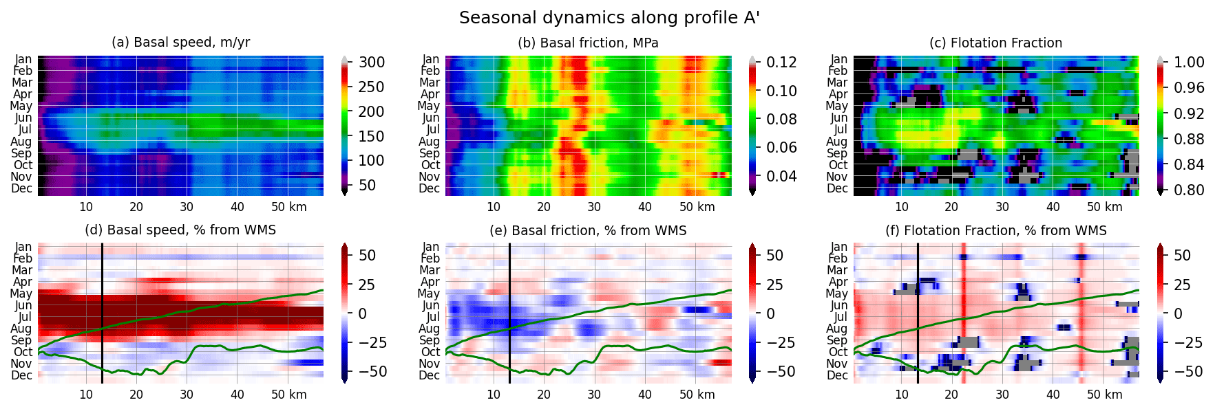
Figure 9Modelled basal speed ub, basal friction τb, and flotation fraction FF along profile A' (see Fig. 1). (a–c) Absolute units and (d–f) fraction relative to the mean winter values (average of January, February, March). In panels (d–f) the vertical black line represents the location of point A plotted in Fig. 6a (see Fig. 1), and the green lines represent the glacier top and bottom surfaces with 5× vertical scale factor. The dark-grey areas in (c) and (f) have no value as they are outside the validity domain of Eq. (13) ().
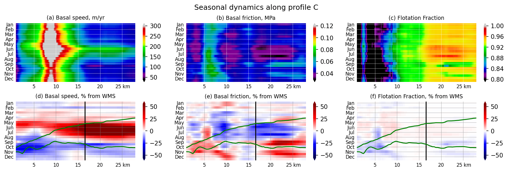
Figure 10Modelled basal speed ub, basal friction τb, and flotation fraction FF along the profile C' (see Fig. 1). (a)–c) Absolute units and (d–f) fraction relative to the mean winter values (average of January, February, March). In panels (d–f) the vertical black line represents the location of point C plotted in Fig. 6c (see Fig. 1), and the green lines represent the glacier top and bottom surfaces with 5× vertical scale factor.
Modelling of the water pressure using subglacial hydrological models (de Fleurian et al., 2016; Koziol and Arnold, 2017; Downs et al., 2018) shows pw spatial patterns similar to those obtained by us: the FF increases with the distance from the margin and is higher in large troughs in the glacier bed. We note however that such hydrological models generally obtain lower water pressure values than estimated here or observed in boreholes, with a typical range of winter FF values of 0.4 to 0.7 across the Russell sector. In de Fleurian et al. (2016), the modelled FF increases significantly in summer compared to the winter mean for altitudes above 1000 m (about 45 km inland from the Insunnguata front line), while below it changes are moderate and mainly concentrated in the Insunnguata valley. While it is difficult from our inversions to draw conclusions on the pressure changes above 1000 m, it seems that the pressure variations below it are more pronounced and systematically higher than modelled by de Fleurian et al. (2016) (this result can also be seen in Figs. 9 and 10), which might suggest that the subglacial hydrological system is not as efficient as assumed in this part of the ice sheet. In other similar work, Downs et al. (2018) reproduced even larger FF variability from summer to winter than we do, adjusting the seasonally evolving hydraulic conductivity. However, they still have absolute values of FF in winter that are almost half of those inferred by us.
5.2.2 Physical processes driving the seasonal dynamics
Isovalues of CN computed from Eq. (13) are reported in Fig. 6 (bottom subplots) for the three particular locations (points A, B, and C) discussed previously. In addition, we show in Figs. 9, 10, and A6 the seasonal evolution of basal velocity, friction, and flotation fraction along three profiles A', C', and B' that pass through points A, C, and B respectively (see Fig. 1).
Points A and B, which we have identified as having a hard bed, are, by assumption, close to the Weertman regime in winter, and they demonstrate that small variations in either ub or τb have a large effect on the magnitude of the retrieved effective pressure.
At point A, the relationship between τb and ub does not follow a power friction law where the evolution of τb would be proportional to such as in Weertman's law (Weertman, 1957). In summer, point A is in a regime closer to Coulomb where changes in N are mainly driven by changes in τb and are fairly insensitive to variations in ub (Fig. 6). In profile A' (Fig. 9), the first 20 km seems to follow the same behaviour as point A, suggesting that the valley bottom behaviour is compatible with a response of the system to local variations in water pressure; i.e. the water pressure increases when the hydrological system is not able to drain the incoming amount of water efficiently and decreases later in the season as the system gets more efficient and/or the flux of water reduces.
In contrast to point A, point B (Fig. 6b) and its surroundings (Fig. A6) follow a power friction law. The variations inferred at point B are relatively compatible with the Weertman regime for the whole year, so it is difficult to discuss the temporal variations in N with confidence (including sharp peaks of CN in Fig. 6b-1). The most plausible hypothesis is that changes in point-B-like areas are mainly driven by changes in longitudinal stresses induced from the accelerating surroundings (such as point A) and are not a response to local variations in water pressure. In detail, we interpret annual friction and ice speed changes at point B as follows: from January to May, the gradual recharge of the subglacial water system locally reduces the friction, and the velocity slowly increases (Van De Wal et al., 2015; Harper et al., 2021). In May, when surface melting begins, local topography and/or organization of the hydrological system do not lead to an increase in water pressure and consequent facilitation of sliding. However, via longitudinal coupling to other accelerating areas such as point A, point B is forced to accelerate as well. Higher sliding speed for a relatively unchanging set of bed properties leads to a higher local friction. That could explain why the friction peak is observed in August at point B when it is the moment of lowest friction at point A. As such, the behaviours at points A and B could also be respectively related to the active and passive regions as have been observed and discussed by Ryser et al. (2014b) or Price et al. (2008). As for the slight increase in velocity from January to March correlated with a decrease in τb, this is consistent with a weakly connected hydrological system that slowly recharges in winter by basal meltwater (Hoffman et al., 2016; Cook et al., 2020).
Beyond 30 km inland, profile A' (Fig. 9) does not follow the bed trough from Insunnguata Sermia and covers higher basal topography where the basal drag alternates between reduced and increased summer values. Along this rugged terrain, the inverted behaviour is probably a mix between point A, where local variations in water pressure occur, and point B, which responds to non-local longitudinal stresses.
Point C is located in a region previously assumed to have a weak bed (see Sect. 5.1.2). The whole 30 km profile C' (Fig. 9) mainly exhibits the same conditions as were described for point C. It follows a topographical valley where the basal friction is very low (<0.05 MPa), the exception being the ridge located at 3 km where basal drag is more important (∼0.07 MPa). As τb and ub are weakly connected to each other in this case, Coulomb-like behaviour is likely approached, where τb would be proportional to the effective pressure during the whole year. In the hypothesis of the hard bed physics used here, this could be consistent with cavitations and therefore low effective pressure throughout the year. Nevertheless, as some reasons should exist to explain the big and numerous cavities open even in winter while the sliding speed here is relatively moderate, we are more inclined to assume the local presence of deforming sediments below the glacier, like those observed in situ by Dow et al. (2013) for another location on Russell Glacier, which shows a τb-vs.-ub relationship similar to our inversions. The exception to this in profile C' is the aforementioned ridge at 3 km, which appears to offer enhanced flow resistance, similar to point B where we have posited the existence of hard-bed physics adjusting to longitudinal stresses. As expected for weak beds, changes in effective pressure are mainly proportional to changes in τb and are weakly sensitive to ub. We observe anti-correlated variations between ub and τb with a maximum in velocity and water pressure in June and a minimum in September; during the winter months, water pressure and velocities increase slowly. As most of this valley is close to flotation throughout the year, the moderate relative increase in water pressure has a large impact on glacier flow in summer as would be expected for a bed described by a Coulomb friction law. These results are compatible with the model of Bougamont et al. (2014) for weak beds, where the water volume and pressure in the sediments increase in the early melt season, leading to a reduction of their shear strength. In late summer and autumn, grain re-arrangement leads to increased porosity, reducing the water pressure and increasing inter-grain contact, resulting in an overall strengthening of the sediment relative to its pre-summer state and thus a maximum friction and a minimum sliding speed in autumn. It is interesting to note that the decrease in sliding velocity at the end of the melt season (August to October depending on the surface altitude) appears in general to be much more pronounced in areas where the bed is described as weak than in the rest of the domain where basal conditions appear to correspond to a hard bed.
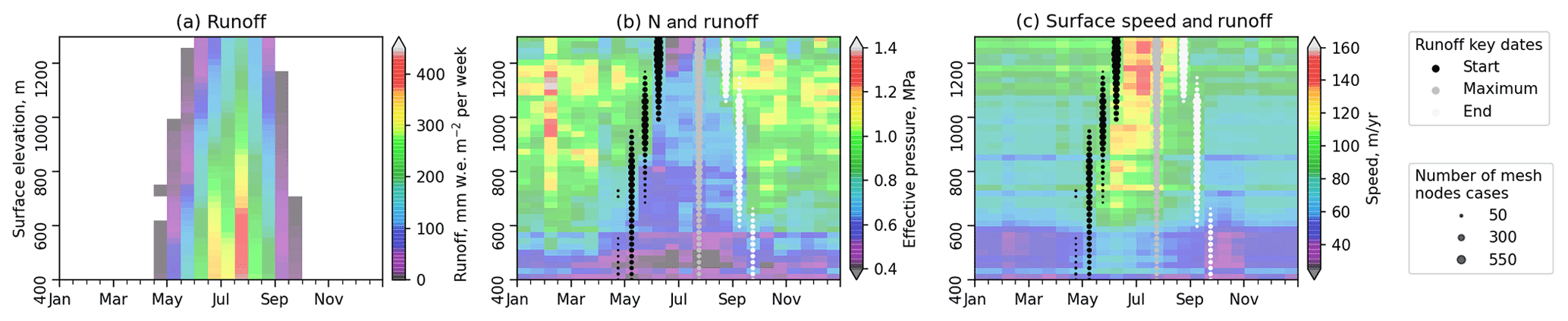
Figure 11Evolution in time and space (averaged over 2 weeks and 20 m elevation bins) of MAR-modelled surface runoff (a), effective pressure N (b), and modelled surface speed us (c). The black, dark grey, and light grey dots represent the onset, maximum, and end of the melting season in (b) and (c). The size of the dots is proportional to the number of mesh nodes found for each state. We define the melting period as runoff >10 mm w.e. m−2 per week.
5.2.3 Comparison with runoff: timing and maximum values
Water pressure variations in the system are globally controlled by the increase in surface runoff that percolates to the glacier bed continuously through moulins or crevasses or sporadically by the drainage of supraglacial lakes (Smith et al., 2015; Stevens et al., 2016). These water pressure variations are therefore closely related to runoff and drainage system evolution. Thus, we compare the seasonal evolution of the runoff obtained from the Regional Atmospheric Model (MAR, https://mar.cnrs.fr/, last access: 7 February 2020) with the inferred effective pressure variations and ice motion acceleration across different altitudes of our model domain (Fig. 11). The runoff is obtained from MAR v3.1, forced by the climate reanalysis ERA5, on a daily basis with a 15 km grid resolution downscaled to 1 km with respect to the surface topography (Fettweis et al., 2020). Further, the period from 2015 to 2019 is averaged in the same way as for the flow velocities (see Sect. 2).
As the domain mostly appears to obey hard-bed physics, the variations in Fig. 11 are most probably mainly characteristic of this type of bed. For all altitudes, the water pressure peaks about 2–4 weeks after the start of the melt season as indicated by the MAR runoff. This delay may be due to water percolation duration (Fountain and Walder, 1998), a sliding activation threshold that is not yet reached (Davison et al., 2019), or simply the fact that the effective pressure changes are still too small to be observed in the 2-week-averaged surface velocities. Ice flow velocity begins to increase at about the same time as the effective pressure decreases. Ice speed quickly reaches its maximum a few weeks later, while runoff continues to increase and is maximal in late July at all altitudes. This probably illustrates the fact that the hydrological system became able to efficiently evacuate the additional meltwater inflow, which does not allow the effective pressure and thus sliding velocity to evolve any further. Once the melt season is over and runoff tends toward zero, the effective pressure quickly returns to its winter state and does not change significantly until next spring. Up to about 1000 m in surface elevation, ice flow experiences a minimum speed that always occurs after the end of the melting season around late September or early October. This seems to correspond to a minimum in water pressure, but, as we are getting closer to the Weertman regime, the pressure values obtained from the inverted basal friction are uncertain.
The overall evolution over the complete year of the surface speed and the water pressure obtained from the inversions corresponds well with the behaviour expected from previous observations and the current understanding of the interaction between the subglacial hydrological system and the ice flow (Nienow et al., 2017; Davison et al., 2019). For instance, the synchronous increase in basal water pressure and surface velocity demonstrated here at the beginning of the melt period fits well with the in situ observations (Bartholomew et al., 2010; Sole et al., 2013; Van De Wal et al., 2015). In our inferred fields the maximum water pressure and velocity are reached while surface runoff still continues to increase, which also corresponds to the local-scale (Bartholomew et al., 2010; Sole et al., 2013) and larger-scale (Sundal et al., 2011; Fitzpatrick et al., 2013) observations in this region, suggesting that a more efficient drainage system is limiting the increase in water pressure at the glacier bed. The drop in water pressure after the end of the melt season (Fig. 11b) corresponds to the presence of a more efficient drainage system established during summer that allows for easy evacuation of the remaining water inputs, chiefly the production of water at the bed as surface melting ceases. Finally, the water pressure slowly increases over winter as the hydrological system becomes inefficient at draining water. Both stages of this evolution have been observed with borehole measurements as well (Van De Wal et al., 2015).
Thus, we conclude that it is possible to obtain robust information on the seasonal evolution of friction and sliding at the base of glaciers by using inverse methods on dense time series of surface flow velocities. Using a pressure-dependent friction law in a suitable and well-restricted framework, it is also realistic to relate these changes in basal conditions to the evolution of the hydrological system and in particular basal water pressure.
5.3 Summary
Spatially extended time series of ice velocity can now be obtained at a time resolution of less than a month, allowing monitoring of glacier motion at a seasonal scale. This offers the opportunity to explore in much more detail the glacier physics driving these changes. Inversions of this time series in the Russell sector indicate that the basal friction changes are mostly consistent with hard-bed physics, which has implications for the choice of friction law in ice flow models and the development of subglacial hydrologic models. In some small areas, the relation between friction and basal sliding rather suggests the presence of weak beds. In such cases we are not able to confidently conclude from our inversions whether this indicates the presence of deformable till, explaining the low strength of the bed, as the results are still compatible with a hard bed with sustained and substantial cavitation.
To relate basal friction and sliding to water pressure, we use a regularized Coulomb friction law designed for a hard bed with cavitation, which seems to give realistic results despite an approximate knowledge of some of the flow law parameters. The results highlight the presence of active (point A) and passive (point B) locations in terms of hydrology. This is similar to the in situ observations made by Ryser et al. (2014b, a) and Young et al. (2019), with the difference that the inversions offer new insight into the large-scale spatial distribution of active and passive sectors over an extended area. Thus, it is possible from such inversions to infer which regions are hydrologically forced during the melt season and relate it to the spatial evolution of the drainage system. It appears that in the Russell area, the main subglacial water pathways are located in the topographic troughs of the bed and thus correspond mainly to the active regions, while the ridges correspond to the passive regions, thus providing additional resistance to enhanced flow in the active regions.
Regardless of pressure assumptions, we show here that inversions of basal conditions from time series of seasonal flow velocity observations provide valuable information on sliding velocity and friction. These inversions could be used to better constrain the results obtained from subglacial hydrology models, as well as to couple these models with ice flow models. We note however that effort is still needed to obtain sufficiently accurate observational data to constrain seasonal variations in friction and sliding above the equilibrium line altitude (ELA) (about 50–60 km from the ice margin in this sector of the ice sheet). In addition, even though the spatial resolution and temporal resolution of the remotely sensed observations seem to be suitable for describing the weekly to monthly evolution of glaciers, it is important to note that the interactions between flow dynamics and subglacial hydrology still occur at much higher frequencies (hourly to daily) that satellite-sensed observations are currently unable to capture, a situation that seems unlikely to change in the coming years. On a more positive note, it nonetheless appears that the time-integrated results we obtain are coherent despite the fact that the effects of the variations are indeed at higher frequencies.
In this paper, we explore the ability of an existing inverse method to use satellite-derived seasonal velocity maps to infer seasonal variations in basal conditions. Based on the observations from multiple satellite missions, we reconstruct the fortnightly seasonal evolution of surface velocity in a land-terminating sector of the ice sheet in southwest Greenland. Then, we invert 24 fortnightly velocity fields to obtain the corresponding evolution of sliding speed and basal friction during a typical year, and we use them to infer the water pressure changes using a pressure-dependent friction law.
The uncertainties in the inverted fields are small compared to the amplitude of the observed variations, which allows the seasonal evolution to be reconstructed and the results to be interpreted in terms of water pressure variations. It seems from the winter inversions that this region of Greenland is globally dominated by a sliding regime described by the physics of hard-rock beds and similarly behaving non-deforming till, with small areas showing characteristics corresponding to beds with Coulomb-type sliding, which can be related to the presence of soft sediments or substantial year-round cavitation over a hard bed. This finding differs from previous results for this region by including both hard-bed (often modelled in a coupled hydrology–ice flow system with a general power law of the form ; see Koziol and Arnold, 2018) and soft-bed (usually modelled with a pure Coulomb law of the form τb=CN; see Bougamont et al., 2014) physics. Indeed, with the proper set of coefficients, depending on their calibration, regularized “Coulomb” friction provides a complete description of both hard and weak regimes of the bed physics.
The obtained water pressure variations are consistent with those expected for both the Weertman-like and Coulomb-like bed and seem to be in phase with the independently derived runoff variations. Thus, we show that inversions of observed surface velocities could serve as an intermediate validation for subglacial hydrology models, assuming that the errors in observed ice dynamics and geometry are small enough to obtain robust inversions. Moreover, the current and future development of space missions suggests that we will be able to perform the observations with sufficient spatial and temporal resolution to describe the weekly to monthly evolution of glacier dynamics on a large scale.
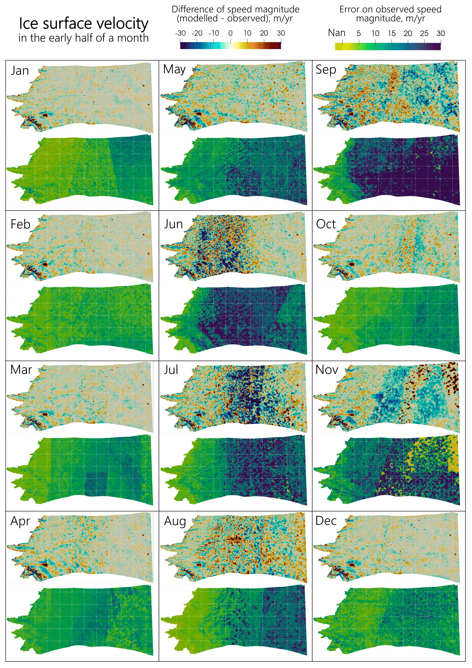
Figure A1Mismatch between modelled and observed velocities (top subplots per section) and error on observed velocities (bottom subplot per section) for the first half of each month. The white grid lines are spaced by 10 km.

Figure A2The data provided by BedMachine v3 (Morlighem et al., 2017): (a) errors on ice thickness and thus bed topography; (b) ice thickness. The white grid lines are spaced by 10 km.
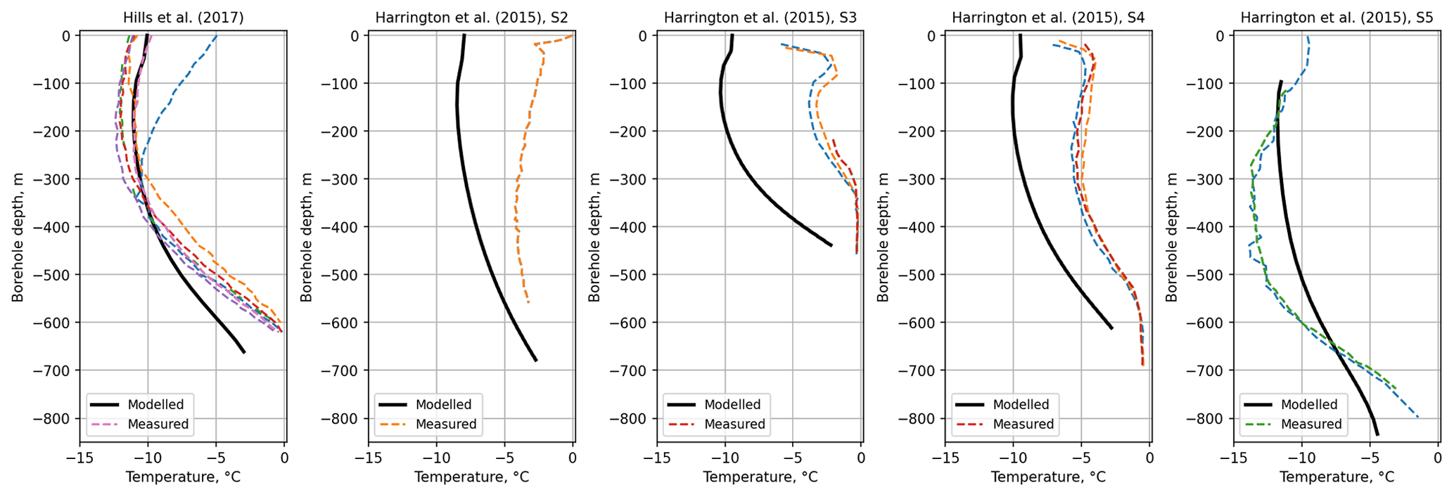
Figure A3Comparison of ice temperature measured in boreholes (Hills et al., 2017; Harrington et al., 2015) with that modelled in SICOPOLIS (Goelzer et al., 2020).
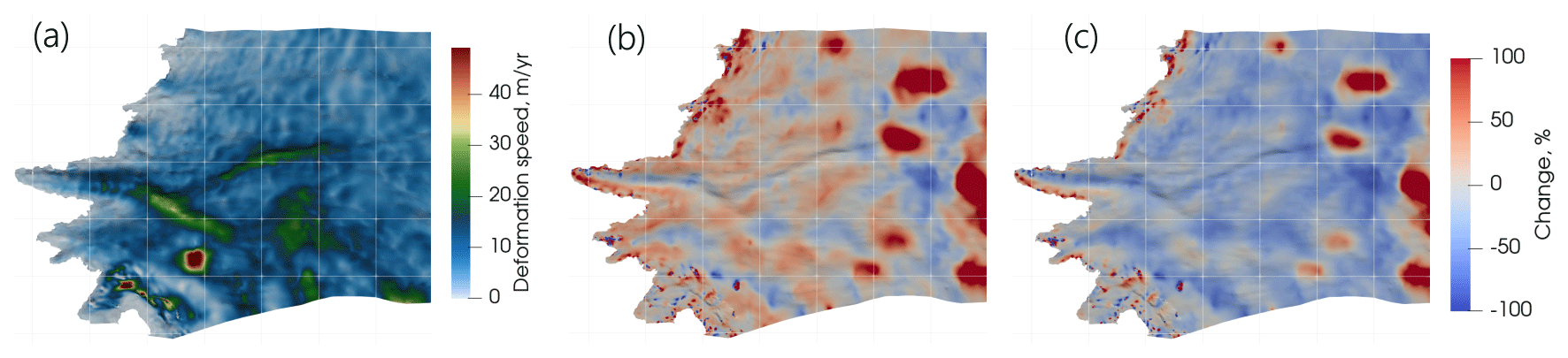
Figure A4(a) Magnitude of modelled deformation velocity in early January. (b) Change in deformation velocity magnitude from early January to early July. (c) Change in fraction given by deformation velocity in total ice surface motion from early January to early July. All maps are with basal topography hillshade added. The white grid lines are spaced by 10 km.
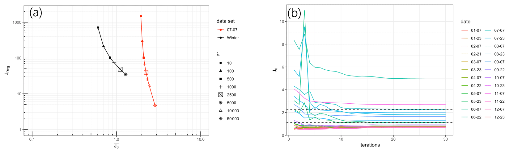
Figure A5(a) L-curves: regularization term (Jreg) as a function of the mismatch between measured and modelled surface speed for different regularization parameters λ. (b) The change in mismatch between measured and modelled surface speed depending on the number of model regularization iterations per twice-monthly data set. Dotted lines represent the J0 values obtained for the mean winter speed (MWS) and early July with chosen λ (2500).

Figure A6Modelled basal speed ub, basal friction τb, and flotation fraction FF along profile B' (see Fig. 1). (a–c) Absolute units and (d–f) fraction relative to the mean winter values (average of January, February, March). In panels (d–f) the vertical black line represents the location of point B plotted in Fig. 6a (see Fig. 1), and the green lines represent the glacier top and bottom surfaces with 5× vertical scale factor. The dark-grey areas in (c) and (f) have no value as they are outside the validity domain of Eq. (13) ().
All data sets used here are publicly available. Elmer/Ice code is available here: http://elmerice.elmerfem.org/ (Elmer/Ice, 2020). BedMachine data are available from Morlighem et al. (2017). GIMP data are available here: https://doi.org/10.5067/NV34YUIXLP9W (Howat et al., 2015). Velocity time series are published at Zenodo (https://doi.org/10.5281/zenodo.5535532; Derkacheva et al., 2021a). Model results for 24 time steps are published at Zenodo (https://doi.org/10.5281/zenodo.5535624, Derkacheva et al., 2021b).
AD processed the velocity data, performed the analysis, wrote the article, and prepared the figures. JM provided supervision, performed the analysis, and wrote the article. FGC provided supervision, designed and performed the Elmer-related processing, and wrote the article. EJ helped to design the Elmer-related processing. NM processed the in situ deformation data and proofread a previous version of the article. SC proofread a previous version of the article. All co-authors helped with discussing and reviewing the article.
The contact author has declared that neither they nor their co-authors have any competing interests.
Publisher's note: Copernicus Publications remains neutral with regard to jurisdictional claims in published maps and institutional affiliations.
Elmer/Ice computations and ice-velocity time series presented in this paper were performed using the https://gricad.univ-grenoble-alpes.fr (last access: 4 October 2021) infrastructure, which is supported by Grenoble research communities. We thank Neil Humphrey for the inclinometry data funded by the NSF Office of Polar Programs-Arctic Natural Sciences awards 1203451 and 0909495, SKB, NWMO, Posiva Oy, and NAGRA.
This research has been supported by the Agence Nationale de la Recherche (grant no. ANR-19-CE01-0011-01) and the CNES MaISON research project.
This paper was edited by Huw Horgan and reviewed by two anonymous referees.
Ahlstrøm, A. P., Petersen, D., Langen, P. L., Citterio, M., and Box, J. E.: Abrupt shift in the observed runoff from the southwestern Greenland ice sheet, Sci. Adv., 3, 1–8, https://doi.org/10.1126/sciadv.1701169, 2017. a
Altena, B. and Kääb, A.: Weekly glacier flow estimation from dense satellite time series using adapted optical flow technology, Front. Earth Sci., 5, 1–12, https://doi.org/10.3389/feart.2017.00053, 2017. a
Arthern, R. J. and Gudmundsson, G. H.: Initialization of ice-sheet forecasts viewed as an inverse Robin problem, J. Glaciol., 56, 527–533, https://doi.org/10.3189/002214310792447699, 2010. a, b
Arthern, R. J., Hindmarsh, R. C. A., and Williams, C. R.: Flow speed within the Antarctic ice sheet and its controls inferred from satellite observations, J. Geophys. Res.-Earth, 120, 1171–1188, https://doi.org/10.1002/2014JF003239, 2015. a
Bartholomew, I., Nienow, P., Mair, D., Hubbard, A., King, M. A., and Sole, A.: Seasonal evolution of subglacial drainage and acceleration in a Greenland outlet glacier, Nat. Geosci., 3, 408–411, https://doi.org/10.1038/ngeo863, 2010. a, b, c
Bartholomew, I., Nienow, P., Sole, A., Mair, D., Cowton, T., and King, M. A.: Short-term variability in Greenland Ice Sheet motion forced by time-varying meltwater drainage: Implications for the relationship between subglacial drainage system behavior and ice velocity, J. Geophys. Res.-Earth, 117, 1–17, https://doi.org/10.1029/2011JF002220, 2012. a
Booth, A. D., Clark, R. A., Kulessa, B., Murray, T., Carter, J., Doyle, S., and Hubbard, A.: Thin-layer effects in glaciological seismic amplitude-versus-angle (AVA) analysis: implications for characterising a subglacial till unit, Russell Glacier, West Greenland, The Cryosphere, 6, 909–922, https://doi.org/10.5194/tc-6-909-2012, 2012. a
Bougamont, M., Christoffersen, P., Hubbard, A. L., Fitzpatrick, A. A., Doyle, S. H., and Carter, S. P.:Sensitive response of the Greenland Ice Sheet to surface melt drainage over a soft bed, Nat. Commun., 5, 5052, https://doi.org/10.1038/ncomms6052, 2014. a, b, c, d
Box, J. E., Fettweis, X., Stroeve, J. C., Tedesco, M., Hall, D. K., and Steffen, K.: Greenland ice sheet albedo feedback: thermodynamics and atmospheric drivers, The Cryosphere, 6, 821–839, https://doi.org/10.5194/tc-6-821-2012, 2012. a
Brinkerhoff, D., Aschwanden, A., and Fahnestock, M.: Constraining subglacial processes from surface velocity observations using surrogate-based Bayesian inference, J. Glaciol., 67, 385–403, https://doi.org/10.1017/jog.2020.112, 2021. a, b
Budd, W. F., Keage, P., and Blundy, N.: Empirical study of ice sliding, J. Glaciol., 2, 157–170, https://doi.org/10.3189/S0022143000029804, 1979. a
Budd, W. F., Jenssen, D., and Smith, I. N.: A Three-Dimensional Time-Dependent Model of the West Antarctic Ice Sheet, Ann. Glaciol., 5, 29–36, https://doi.org/10.3189/1984AoG5-1-29-36, 1984. a
Cabral, B. and Leedom, L. C.: Imaging Vector Fields Using Line Integral Convolution, in: Proceedings of ACM SIGGRAPH'93, Anaheim, 263–270, https://doi.org/10.1145/166117.166151, 1993. a
Christoffersen, P., Bougamont, M., Hubbard, A., Doyle, S. H., Grigsby, S., and Pettersson, R.: Cascading lake drainage on the Greenland Ice Sheet triggered by tensile shock and fracture, Nat. Commun., 9, 1064, https://doi.org/10.1038/s41467-018-03420-8, 2018. a, b
Cleveland, W. S.: Robust locally weighted regression and smoothing scatterplots, J. Am. Stat. Assoc., 74, 829–836, https://doi.org/10.1080/01621459.1979.10481038, 1979. a
Cleveland, W. S. and Devlin, S. J.: Locally weighted regression: An approach to regression analysis by local fitting, J. Am. Stat. Assoc., 83, 596–610, https://doi.org/10.1080/01621459.1988.10478639, 1988. a
Cook, S. J., Christoffersen, P., Todd, J., Slater, D., and Chauché, N.: Coupled modelling of subglacial hydrology and calving-front melting at Store Glacier, West Greenland, The Cryosphere, 14, 905–924, https://doi.org/10.5194/tc-14-905-2020, 2020. a, b, c
Cook, S. J., Christoffersen, P., and Todd, J.: A fully-coupled 3D model of a large Greenlandic outlet glacier with evolving subglacial hydrology, frontal plume melting and calving, J. Glaciol., https://doi.org/10.1017/jog.2021.109, in press, 2021. a
Cowton, T., Sole, A., Nienow, P., Slater, D., Wilton, D., and Hanna, E.: Controls on the transport of oceanic heat to Kangerdlugssuaq Glacier, East Greenland, J. Glaciol., 62, 1167–1180, https://doi.org/10.1017/jog.2016.117, 2016. a
Csatho, B. M., Schenka, A. F., Van Der Veen, C. J., Babonis, G., Duncan, K., Rezvanbehbahani, S., Van Den Broeke, M. R., Simonsen, S. B., Nagarajan, S., and Van Angelen, J. H.: Laser altimetry reveals complex pattern of Greenland Ice Sheet dynamics, P. Natl. Acad. Sci. USA, 111, 18478–18483, https://doi.org/10.1073/pnas.1411680112, 2014. a
Cuffey, K. and Paterson, W.: The physics of glaciers, Academic Press, Amsterdam, 2010. a
Dapogny, C., Dobrzynski, C., and Frey, P.: Three-dimensional adaptive domain remeshing, implicit domain meshing, and applications to free and moving boundary problems, J. Comput. Phys., 262, 358–378, https://doi.org/10.1016/j.jcp.2014.01.005, 2014. a
Davison, B. J., Sole, A. J., Livingstone, S. J., Cowton, T. R., and Nienow, P. W.: The Influence of Hydrology on the Dynamics of Land-Terminating Sectors of the Greenland Ice Sheet, Front. Earth Sci., 7, 1–24, https://doi.org/10.3389/feart.2019.00010, 2019. a, b, c, d
de Fleurian, B., Morlighem, M., Seroussi, H., Rignot, E., van den Broeke, M. R., Kuipers Munneke, P., Mouginot, J., Smeets, P. C. J. P., and Tedstone, A. J.: A modeling study of the effect of runoff variability on the effective pressure beneath Russell Glacier, West Greenland, J. Geophys. Res.-Earth, 121, 1834–1848, https://doi.org/10.1002/2016JF003842, 2016. a, b, c, d, e
De Fleurian, B., Werder, M. A., Beyer, S., Brinkerhoff, D. J., Delaney, I., Dow, C. F., Downs, J., Gagliardini, O., Hoffman, M. J., Hooke, R. L., Seguinot, J., and Sommers, A. N.: SHMIP the subglacial hydrology model intercomparison Project, J. Glaciology, 64, 897–916, https://doi.org/10.1017/jog.2018.78, 2018. a
Derkacheva, A., Mouginot, J., Millan, R., Maier, N., and Gillet-Chaulet, F.: Data Reduction Using Statistical and Regression Approaches for Ice Velocity Derived by Landsat-8, Sentinel-1 and Sentinel-2, Remote Sens., 12, 1935, https://doi.org/10.3390/rs12121935, 2020. a, b, c
Derkacheva, A., Mouginot, J., and Millan, R.: Satellite-observed surface flow speed within Russell sector, West Greenland, bi-weekly average of 2015–2019 (1.0), Zenodo [data set], https://doi.org/10.5281/zenodo.5535532, 2021a. a
Derkacheva, A., Gillet-Chaulet, F., and Mouginot, J.: Seasonal evolution of basal conditions within Russell sector, West Greenland, inverted from satellite observations of surface flow (1.0), Zenodo [data set], https://doi.org/10.5281/zenodo.5535624, 2021b. a
Dow, C., Hubbard, A., Booth, A., Doyle, S., Gusmeroli, A., and Kulessa, B.: Seismic evidence of mechanically weak sediments underlying Russell Glacier, West Greenland, Ann. Glaciol., 54, 135–141, https://doi.org/10.3189/2013AoG64A032, 2013. a, b, c, d, e
Downs, J. Z., Johnson, J. V., Harper, J. T., Meierbachtol, T., and Werder, M. A.: Dynamic Hydraulic Conductivity Reconciles Mismatch Between Modeled and Observed Winter Subglacial Water Pressure, J. Geophys. Res.-Earth, 123, 818–836, https://doi.org/10.1002/2017JF004522, 2018. a, b, c, d, e
Doyle, S. H., Hubbard, A., Van De Wal, R. S., Box, J. E., Van As, D., Scharrer, K., Meierbachtol, T. W., Smeets, P. C., Harper, J. T., Johansson, E., Mottram, R. H., Mikkelsen, A. B., Wilhelms, F., Patton, H., Christoffersen, P., and Hubbard, B.: Amplified melt and flow of the Greenland ice sheet driven by late-summer cyclonic rainfall, Nat. Geosci., 8, 647–653, https://doi.org/10.1038/ngeo2482, 2015. a
Edwards, T. L., Fettweis, X., Gagliardini, O., Gillet-Chaulet, F., Goelzer, H., Gregory, J. M., Hoffman, M., Huybrechts, P., Payne, A. J., Perego, M., Price, S., Quiquet, A., and Ritz, C.: Effect of uncertainty in surface mass balance-elevation feedback on projections of the future sea level contribution of the Greenland ice sheet, The Cryosphere, 8, 195–208, https://doi.org/10.5194/tc-8-195-2014, 2014. a
Elmer/Ice: Open Source Finite Element Software for Ice Sheet, Glaciers and Ice Flow Modelling, Elmer/Ice [code], http://elmerice.elmerfem.org/, last access: 21 February 2020. a
Fahnestock, M., Scambos, T., Moon, T., Gardner, A., Haran, T., and Klinger, M.: Rapid large-area mapping of ice flow using Landsat 8, Remote Sens. Environ., 185, 84–94, https://doi.org/10.1016/j.rse.2015.11.023, 2016. a
Fettweis, X., Hofer, S., Krebs-Kanzow, U., Amory, C., Aoki, T., Berends, C. J., Born, A., Box, J. E., Delhasse, A., Fujita, K., Gierz, P., Goelzer, H., Hanna, E., Hashimoto, A., Huybrechts, P., Kapsch, M.-L., King, M. D., Kittel, C., Lang, C., Langen, P. L., Lenaerts, J. T. M., Liston, G. E., Lohmann, G., Mernild, S. H., Mikolajewicz, U., Modali, K., Mottram, R. H., Niwano, M., Noël, B., Ryan, J. C., Smith, A., Streffing, J., Tedesco, M., van de Berg, W. J., van den Broeke, M., van de Wal, R. S. W., van Kampenhout, L., Wilton, D., Wouters, B., Ziemen, F., and Zolles, T.: GrSMBMIP: intercomparison of the modelled 1980–2012 surface mass balance over the Greenland Ice Sheet, The Cryosphere, 14, 3935–3958, https://doi.org/10.5194/tc-14-3935-2020, 2020. a
Fitzpatrick, A. A., Hubbard, A., Joughin, I., Quincey, D. J., As, D. V., Mikkelsen, A. P., Doyle, S. H., Hasholt, B., and Jones, G. A.: Ice flow dynamics and surface meltwater flux at a land-terminating sector of the Greenland ice sheet, J. Glaciol., 59, 687–696, https://doi.org/10.3189/2013JoG12J143, 2013. a, b
Flowers, G. E.: Modelling water flow under glaciers and ice sheets, P. Roy. Soc. A, 471, 20140907, https://doi.org/10.1098/rspa.2014.0907, 2015. a
Fountain, A. G. and Walder, J. S.: Water flow through temperate glaciers, Rev. Geophys., 36, 299–328, https://doi.org/10.1029/97RG03579, 1998. a
Fowler, A. C.: On the rheology of till, Ann. Glaciol., 37, 55–59, https://doi.org/10.3189/172756403781815951, 2003. a
Gagliardini, O. and Meyssonnier, J.: Lateral boundary conditions for a local anisotropic ice-flow model, Ann. Glaciol., 35, 503–509, https://doi.org/10.3189/172756402781817202, 2002. a
Gagliardini, O. and Werder, M. A.: Influence of increasing surface melt over decadal timescales on land-terminating Greenland-type outlet glaciers, J. Glaciol., 64, 700–710, https://doi.org/10.1017/jog.2018.59, 2018. a, b, c, d
Gagliardini, O., Cohen, D., Råback, P., and Zwinger, T.: Finite-element modeling of subglacial cavities and related friction law, J. Geophys. Res., 112, F02027, https://doi.org/10.1029/2006JF000576, 2007. a, b, c, d
Gagliardini, O., Zwinger, T., Gillet-Chaulet, F., Durand, G., Favier, L., de Fleurian, B., Greve, R., Malinen, M., Martín, C., Råback, P., Ruokolainen, J., Sacchettini, M., Schäfer, M., Seddik, H., and Thies, J.: Capabilities and performance of Elmer/Ice, a new-generation ice sheet model, Geosci. Model Dev., 6, 1299–1318, https://doi.org/10.5194/gmd-6-1299-2013, 2013. a, b, c
Gilbert, J. C. and Lemaréchal, C.: Some numerical experiments with variable-storage quasi-Newton algorithms, Math. Program., 45, 407–435, https://doi.org/10.1007/BF01589113, 1989. a
Gillet-Chaulet, F., Gagliardini, O., Seddik, H., Nodet, M., Durand, G., Ritz, C., Zwinger, T., Greve, R., and Vaughan, D. G.: Greenland ice sheet contribution to sea-level rise from a new-generation ice-sheet model, The Cryosphere, 6, 1561–1576, https://doi.org/10.5194/tc-6-1561-2012, 2012. a
Gillet-Chaulet, F., Durand, G., Gagliardini, O., Mosbeux, C., Mouginot, J., Rémy, F., and Ritz, C.: Assimilation of surface velocities acquired between 1996 and 2010 to constrain the form of the basal friction law under Pine Island Glacier, Geophys. Res. Lett., 43, 10311–10321, https://doi.org/10.1002/2016GL069937, 2016. a
Goelzer, H., Robinson, A., Seroussi, H., and van de Wal, R. S.: Recent Progress in Greenland Ice Sheet Modelling, Curr. Clim. Change Rep., 3, 291–302, https://doi.org/10.1007/s40641-017-0073-y, 2017. a
Goelzer, H., Nowicki, S., Payne, A., Larour, E., Seroussi, H., Lipscomb, W. H., Gregory, J., Abe-Ouchi, A., Shepherd, A., Simon, E., Agosta, C., Alexander, P., Aschwanden, A., Barthel, A., Calov, R., Chambers, C., Choi, Y., Cuzzone, J., Dumas, C., Edwards, T., Felikson, D., Fettweis, X., Golledge, N. R., Greve, R., Humbert, A., Huybrechts, P., Le Clec'h, S., Lee, V., Leguy, G., Little, C., Lowry, D., Morlighem, M., Nias, I., Quiquet, A., Rückamp, M., Schlegel, N. J., Slater, D. A., Smith, R., Straneo, F., Tarasov, L., Van De Wal, R., and Van Den Broeke, M.: The future sea-level contribution of the Greenland ice sheet: A multi-model ensemble study of ISMIP6, The Cryosphere, 14, 3071–3096, https://doi.org/10.5194/tc-14-3071-2020, 2020. a, b
Greskowiak, J.: Tide-induced salt-fingering flow during submarine groundwater discharge, Geophys. Res. Lett., 41, 6413–6419, https://doi.org/10.1002/2014GL061184, 2014. a, b, c
Habermann, M., Maxwell, D., and Truffer, M.: Reconstruction of basal properties in ice sheets using iterative inverse methods, J. Glaciol., 58, 795–807, https://doi.org/10.3189/2012JoG11J168, 2012. a
Habermann, M., Truffer, M., and Maxwell, D.: Error sources in basal yield stress inversions for Jakobshavn Isbræ, Greenland, derived from residual patterns of misfit to observations, J. Glaciol., 63, 999–1011, https://doi.org/10.1017/jog.2017.61, 2017. a
Hansen, P. C.: The L-Curve and its Use in the Numerical Treatment of Inverse Problems, in: Computational Inverse Problems in Electrocardiology, edited by: Johnston, P., WIT Press, 119–142, 2001. a
Harper, J., Meierbachtol, T., Humphrey, N., Saito, J., and Stansberry, A.: Variability of Basal Meltwater Generation During Winter, Western Greenland Ice Sheet, The Cryosphere Discuss. [preprint], https://doi.org/10.5194/tc-2021-179, in review, 2021. a
Harper, J. T., Humphrey, N. F., Meierbachtol, T. W., Graly, J. A., and Fischer, U. H.: Borehole measurements indicate hard bed conditions, Kangerlussuaq sector, western Greenland Ice Sheet, J. Geophys. Res.-Earth, 122, 1605–1618, https://doi.org/10.1002/2017JF004201, 2017. a, b, c, d
Harrington, J. A., Humphrey, N. F., and Harper, J. T.: Temperature distribution and thermal anomalies along a flowline of the Greenland ice sheet, Ann. Glaciol., 56, 98–104, https://doi.org/10.3189/2015AoG70A945, 2015. a, b, c, d
Helanow, C., Iverson, N. R., Woodard, J. B., and Zoet, L. K.: A slip law for hard-bedded glaciers derived from observed bed topography, Sci. Adv., 7, eabe7798, https://doi.org/10.1126/sciadv.abe7798, 2021. a
Helm, V., Humbert, A., and Miller, H.: Elevation and elevation change of Greenland and Antarctica derived from CryoSat-2, The Cryosphere, 8, 1539–1559, https://doi.org/10.5194/tc-8-1539-2014, 2014. a
Hewitt, I. J.: Seasonal changes in ice sheet motion due to melt water lubrication, Earth Planet. Sc. Lett., 371–372, 16–25, https://doi.org/10.1016/j.epsl.2013.04.022, 2013. a, b, c, d, e
Hills, B. H., Harper, J. T., Humphrey, N. F., and Meierbachtol, T. W.: Measured Horizontal Temperature Gradients Constrain Heat Transfer Mechanisms in Greenland Ice, Geophys. Res. Lett., 44, 9778–9785, https://doi.org/10.1002/2017GL074917, 2017. a, b, c, d
Hoffman, M. J., Andrews, L. C., Price, S. A., Catania, G. A., Neumann, T. A., Lüthi, M. P., Gulley, J., Ryser, C., Hawley, R. L., and Morriss, B.: Greenland subglacial drainage evolution regulated by weakly connected regions of the bed, Nat. Commun., 7, 13903, https://doi.org/10.1038/ncomms13903, 2016. a, b, c
Howat, I., Negrete, A., and Smith, B.: MEaSUREs Greenland Ice Mapping Project (GIMP) Digital Elevation Model (2.1), NASA National Snow and Ice Data Center Distributed Active Archive Center, Boulder, Colorado, USA, [data set], https://doi.org/10.5067/NV34YUIXLP9W, 2015. a
Howat, I. M., Negrete, A., and Smith, B. E.: The Greenland Ice Mapping Project (GIMP) land classification and surface elevation data sets, The Cryosphere, 8, 1509–1518, https://doi.org/10.5194/tc-8-1509-2014, 2014. a, b
Iken, A.: The effect of the subglacial water pressure on the sliding velocity of a glacier in an idealized numerical model, J. Glaciol., 27, 407–421, https://doi.org/10.1017/S0022143000011448, 1981. a, b, c
Iverson, N. R.: Shear resistance and continuity of subglacial till: Hydrology rules, J. Glaciol., 56, 1104–1114, https://doi.org/10.3189/002214311796406220, 2011. a
Iverson, N. R., Hooyer, T. S., and Baker, R. W.: Ring-shear studies of till deformation: Coulomb-plastic behavior and distributed strain in glacier beds, J. Glaciol., 44, 634–642, https://doi.org/10.1017/S0022143000002136, 1998. a, b
Jay-Allemand, M., Gillet-Chaulet, F., Gagliardini, O., and Nodet, M.: Investigating changes in basal conditions of Variegated Glacier prior to and during its 1982–1983 surge, The Cryosphere, 5, 659–672, https://doi.org/10.5194/tc-5-659-2011, 2011. a, b, c
Joughin, I., MacAyeal, D. R., and Tulaczyk, S.: Basal shear stress of the Ross ice streams from control method inversions, J. Geophys. Res.-Solid, 109, 1–20, https://doi.org/10.1029/2003JB002960, 2004. a
Joughin, I., Das, S. B., King, M. A., Smith, B. E., and Howat, I. M.: Seasonal Speedup Along the Western Flank of the Greenland Ice Sheet, Science, 320, 781–783, 2008. a
Joughin, I., Smith, B. E., and Howat, I.: Greenland Ice Mapping Project: ice flow velocity variation at sub-monthly to decadal timescales, The Cryosphere, 12, 2211–2227, https://doi.org/10.5194/tc-12-2211-2018, 2018. a
Joughin, I., Smith, B. E., and Schoof, C. G.: Regularized Coulomb Friction Laws for Ice Sheet Sliding: Application to Pine Island Glacier, Antarctica, Geophys. Res. Lett., 46, 4764–4771, https://doi.org/10.1029/2019GL082526, 2019. a, b
Koziol, C. P. and Arnold, N.: Incorporating modelled subglacial hydrology into inversions for basal drag, The Cryosphere, 11, 2783–2797, https://doi.org/10.5194/tc-11-2783-2017, 2017. a, b, c, d, e, f
Koziol, C. P. and Arnold, N.: Modelling seasonal meltwater forcing of the velocity of land-terminating margins of the Greenland Ice Sheet, The Cryosphere, 12, 971–991, https://doi.org/10.5194/tc-12-971-2018, 2018. a, b, c, d, e
Kulessa, B., Hubbard, A. L., Booth, A. D., Bougamont, M., Dow, C. F., Doyle, S. H., Christoffersen, P., Lindbäck, K., Pettersson, R., Fitzpatrick, A. A. W., and Jones, G. A.: Seismic evidence for complex sedimentary control of Greenland Ice Sheet flow, Sci. Adv., 3, e1603071, https://doi.org/10.1126/sciadv.1603071, 2017. a, b, c
Larour, E., Utke, J., Csatho, B., Schenk, A., Seroussi, H., Morlighem, M., Rignot, E., Schlegel, N., and Khazendar, A.: Inferred basal friction and surface mass balance of the Northeast Greenland Ice Stream using data assimilation of ICESat (Ice Cloud and land Elevation Satellite) surface altimetry and ISSM (Ice Sheet System Model), The Cryosphere, 8, 2335–2351, https://doi.org/10.5194/tc-8-2335-2014, 2014. a
Le Clec'h, S., Charbit, S., Quiquet, A., Fettweis, X., Dumas, C., Kageyama, M., Wyard, C., and Ritz, C.: Assessment of the Greenland ice sheet-atmosphere feedbacks for the next century with a regional atmospheric model coupled to an ice sheet model, The Cryosphere, 13, 373–395, https://doi.org/10.5194/tc-13-373-2019, 2019. a
Lemos, A., Shepherd, A., McMillan, M., and Hogg, A.: Seasonal Variations in the Flow of Land-Terminating Glaciers in Central-West Greenland Using Sentinel-1 Imagery, Remote Sens., 10, 1878, https://doi.org/10.3390/rs10121878, 2018. a, b
Lindbäck, K., Pettersson, R., Doyle, S. H., Helanow, C., Jansson, P., Kristensen, S. S., Stenseng, L., Forsberg, R., and Hubbard, A. L.: High-resolution ice thickness and bed topography of a land-terminating section of the Greenland Ice Sheet, Earth Syst. Sci. Data, 6, 331–338, https://doi.org/10.5194/essd-6-331-2014, 2014. a
MacAyeal, D. R.: A tutorial on the use of control methods in ice-sheet modeling, J. Glaciol., 39, 91–98, https://doi.org/10.1017/S0022143000015744, 1993. a
Maier, N., Humphrey, N., Harper, J., and Meierbachtol, T.: Sliding dominates slow-flowing margin regions, Greenland Ice Sheet, Sci. Adv., 5, eaaw5406, https://doi.org/10.1126/sciadv.aaw5406, 2019. a, b, c, d, e, f, g, h, i
Maier, N., Gimbert, F., Gillet-Chaulet, F., and Gilbert, A.: Basal traction mainly dictated by hard-bed physics over grounded regions of Greenland, The Cryosphere, 15, 1435–1451, https://doi.org/10.5194/tc-15-1435-2021, 2021a. a, b, c, d, e
Maier, N., Humphrey, N., Meierbachtol, T., and Harper, J.: Deformation motion tracks sliding changes through summer, western Greenland, J. Glaciol., https://doi.org/10.1017/jog.2021.87, in press, 2021b. a
Mangeney, A., Califano, F., and Castelnau, O.: Isothermal flow of an anisotropic ice sheet in the vicinity of an ice divide, J. Geophys. Res.-Solid, 101, 28189–28204, https://doi.org/10.1029/96jb01924, 1996. a
Meierbachtol, T., Harper, J., and Humphrey, N.: Basal drainage system response to increasing surface melt on the Greenland ice sheet, Science, 341, 777–779, https://doi.org/10.1126/science.1235905, 2013. a, b, c, d
Mikkelsen, A. B., Hubbard, A., Macferrin, M., Box, J. E., Doyle, S. H., Fitzpatrick, A., Hasholt, B., Bailey, H. L., Lindbäck, K., and Pettersson, R.: Extraordinary runoff from the Greenland ice sheet in 2012 amplified by hypsometry and depleted firn retention, The Cryosphere, 10, 1147–1159, https://doi.org/10.5194/tc-10-1147-2016, 2016. a
Millan, R., Mouginot, J., Rabatel, A., Jeong, S., Cusicanqui, D., Derkacheva, A., and Chekki, M.: Mapping surface flow velocity of glaciers at regional scale using a multiple sensors approach, Remote Sens., 11, 1–21, https://doi.org/10.3390/rs11212498, 2019. a
Minchew, B., Simons, M., Björnsson, H., Pálsson, F., Morlighem, M., Seroussi, H., Larour, E., and Hensley, S.: Plastic bed beneath Hofsjökull ice cap, central Iceland, and the sensitivity of ice flow to surface meltwater flux, J. Glaciol., 62, 147–158, https://doi.org/10.1017/jog.2016.26, 2016. a
Morlighem, M., Rignot, E., Seroussi, H., Larour, E., Ben Dhia, H., and Aubry, D.: A mass conservation approach for mapping glacier ice thickness, Geophys. Res. Lett., 38, 1–6, https://doi.org/10.1029/2011GL048659, 2011. a
Morlighem, M., Rignot, E., Mouginot, J., Wu, X., Seroussi, H., Larour, E., and Paden, J.: High-resolution bed topography mapping of Russell Glacier, Greenland, inferred from Operation IceBridge data, J. Glaciol., 59, 1015–1023, https://doi.org/10.3189/2013JoG12J235, 2013. a
Morlighem, M., Williams, C. N., Rignot, E., An, L., Arndt, J. E., Bamber, J. L., Catania, G., Chauché, N., Dowdeswell, J. A., Dorschel, B., Fenty, I., Hogan, K., Howat, I., Hubbard, A., Jakobsson, M., Jordan, T. M., Kjeldsen, K. K., Millan, R., Mayer, L., Mouginot, J., Noël, B. P., O'Cofaigh, C., Palmer, S., Rysgaard, S., Seroussi, H., Siegert, M. J., Slabon, P., Straneo, F., van den Broeke, M. R., Weinrebe, W., Wood, M., and Zinglersen, K. B.: BedMachine v3: Complete Bed Topography and Ocean Bathymetry Mapping of Greenland From Multibeam Echo Sounding Combined With Mass Conservation, Geophys. Res. Lett., 44, 11051–11061, https://doi.org/10.1002/2017GL074954, 2017. a, b, c, d, e
Mouginot, J., Rignot, E., Scheuchl, B., and Millan, R.: Comprehensive Annual Ice Sheet Velocity Mapping Using Landsat-8, Sentinel-1, and RADARSAT-2 Data, Remote Sen., 9, 1–20, https://doi.org/10.3390/rs9040364, 2017. a, b, c
Mouginot, J., Rignot, E., Bjørk, A. A., van den Broeke, M., Millan, R., Morlighem, M., Noël, B., Scheuchl, B., and Wood, M.: Forty-six years of Greenland Ice Sheet mass balance from 1972 to 2018, P. Natl. Acad. Sci. USA, 116, 9239–9244, https://doi.org/10.1073/pnas.1904242116, 2019. a
Nienow, P. W., Sole, A. J., Slater, D. A., and Cowton, T. R.: Recent Advances in Our Understanding of the Role of Meltwater in the Greenland Ice Sheet System, Curr. Clim. Change Rep., 3, 330–344, https://doi.org/10.1007/s40641-017-0083-9, 2017. a, b, c
Palmer, S., Shepherd, A., Nienow, P., and Joughin, I.: Seasonal speedup of the Greenland Ice Sheet linked to routing of surface water, Earth Planet. Sc. Lett., 302, 423–428, https://doi.org/10.1016/j.epsl.2010.12.037, 2011. a, b, c
Pimentel, S., Flowers, G. E., and Schoof, C. G.: A hydrologically coupled higher-order flow-band model of ice dynamics with a Coulomb friction sliding law, J. Geophys. Res.-Earth, 115, 1–16, https://doi.org/10.1029/2009JF001621, 2010. a
Poinar, K., Joughin, I., Das, S. B., Behn, M. D., Lenaerts, J. T., and Van Den Broeke, M. R.: Limits to future expansion of surface-melt-enhanced ice flow into the interior of western Greenland, Geophys. Res. Lett., 42, 1800–1807, https://doi.org/10.1002/2015GL063192, 2015. a
Price, S. F., Payne, A. J., Catania, G. A., and Neumann, T. A.: Seasonal acceleration of inland ice via longitudinal coupling to marginal ice, J. Glaciol., 54, 213–219, https://doi.org/10.3189/002214308784886117, 2008. a
Rignot, E. and Mouginot, J.: Ice flow in Greenland for the International Polar Year 2008–2009, Geophys. Res. Lett., 39, 1–7, https://doi.org/10.1029/2012GL051634, 2012. a
Ryser, C., Lüthi, M. P., Andrews, L. C., Catania, G. A., Funk, M., and Hawley, R.: Caterpillar-like ice motion in the ablation zone of the Greenland ice sheet, J. Geophys. Res.-Earth, 119, 2258–2271, https://doi.org/10.1002/2013JF003067, 2014a. a
Ryser, C., Luthi, M. P., Andrews, L. C., Hoffman, M. J., Catania, G. A., Hawley, R. L., Neumann, T. A., and Kristensen, S. S.: Sustained high basal motion of the Greenland ice sheet revealed by borehole deformation, J. Glaciol., 60, 647–660, https://doi.org/10.3189/2014JoG13J196, 2014b. a, b
Scambos, T. A. and Haran, T.: An image-enhanced DEM of the Greenland ice sheet, Ann. Glaciol., 34, 291–298, https://doi.org/10.3189/172756402781817969, 2002. a
Schäfer, M., Gillet-Chaulet, F., Gladstone, R., Pettersson, R., Pohjola, V. A., Strozzi, T., and Zwinger, T.: Assessment of heat sources on the control of fast flow of Vestfonna ice cap, Svalbard, The Cryosphere, 8, 1951–1973, https://doi.org/10.5194/tc-8-1951-2014, 2014. a
Schoof, C.: The effect of cavitation on glacier sliding, P. Roy. Soc. A, 461, 609–627, https://doi.org/10.1098/rspa.2004.1350, 2005. a, b, c, d
Shapero, D. R., Joughin, I. R., Poinar, K., Morlighem, M., and Gillet-Chaulet, F.: Basal resistance for three of the largest Greenland outlet glaciers, J. Geophys. Res.-Earth, 121, 168–180, https://doi.org/10.1002/2015JF003643, 2016. a
Smeets, C. J. P. P., Boot, W., Hubbard, A., Pettersson, R., Wilhelms, F., Van Den Broeke, M. R., and Van De Wal, R. S. W.: A wireless subglacial probe for deep ice applications, Instrum. Meth., 58, 841–848, https://doi.org/10.3189/2012JoG11J130, 2012. a, b, c
Smith, L. C., Chu, V. W., Yang, K., Gleason, C. J., Pitcher, L. H., Rennermalm, A. K., Legleiter, C. J., Behar, A. E., Overstreet, B. T., Moustafa, S. E., Tedesco, M., Forster, R. R., LeWinter, A. L., Finnegan, D. C., Sheng, Y., and Balog, J.: Efficient meltwater drainage through supraglacial streams and rivers on the southwest Greenland ice sheet, P. Natl. Acad. Sci. USA, 112, 1001–1006, https://doi.org/10.1073/pnas.1413024112, 2015. a
Sole, A., Nienow, P., Bartholomew, I., Mair, D., Cowton, T., Tedstone, A., and King, M. A.: Winter motion mediates dynamic response of the Greenland Ice Sheet to warmer summers, Geophys. Res. Lett., 40, 3940–3944, https://doi.org/10.1002/grl.50764, 2013. a, b
Stevens, L. A., Behn, M. D., Das, S. B., Joughin, I., Noël, B. P., van den Broeke, M. R., and Herring, T.: Greenland Ice Sheet flow response to runoff variability, Geophys. Res. Lett., 43, 11295–11303, https://doi.org/10.1002/2016GL070414, 2016. a, b
Sugiyama, S. and Gudmundsson, G. H.: Short-term variations in glacier flow controlled by subglacial water pressure at Lauteraargletscher, Bernese Alps, Switzerland, J. Glaciol., 50, 353–362, https://doi.org/10.3189/172756504781829846, 2004. a
Sundal, A. V., Shepherd, A., Nienow, P., Hanna, E., Palmer, S., and Huybrechts, P.: Melt-induced speed-up of Greenland ice sheet offset by efficient subglacial drainage, Nature, 469, 521–524, https://doi.org/10.1038/nature09740, 2011. a
Tedstone, A., Nienow, P. W., Gourmelen, N., Dehecq, A., Goldberg, D., and Hanna, E.: Decadal slowdown of a land-terminating sector of the Greenland Ice Sheet despite warming, Nature, 526, 692–695, https://doi.org/10.1038/nature15722, 2015. a, b
Tedstone, A. J., Nienow, P. W., Sole, A. J., Mair, D. W. F., Cowton, T. R., Bartholomew, I. D., and King, M. A.: Greenland ice sheet motion insensitive to exceptional meltwater forcing, P. Natl. Acad. Sci. USA, 110, 19719–19724, https://doi.org/10.1073/pnas.1315843110, 2013. a
Tedstone, A. J., Nienow, P. W., Gourmelen, N., and Sole, A. J.: Greenland ice sheet annual motion insensitive to spatial variations in subglacial hydraulic structure, Geophys. Res. Lett., 41, 8910–8917, https://doi.org/10.1002/2014GL062386, 2014. a
Truffer, M., Harrison, W. D., and Echelmeyer, K. A.: Glacier motion dominated by processes deep in underlying till, J. Glaciol., 46, 213–221, https://doi.org/10.3189/172756500781832909, 2000. a
Trusel, L. D., Das, S. B., Osman, M. B., Evans, M. J., Smith, B. E., Fettweis, X., McConnell, J. R., Noël, B. P., and van den Broeke, M. R.: Nonlinear rise in Greenland runoff in response to post-industrial Arctic warming, Nature, 564, 104–108, https://doi.org/10.1038/s41586-018-0752-4, 2018. a
Van De Wal, R. S., Boot, W., Smeets, C. J., Snellen, H., Van Den Broeke, M. R., and Oerlemans, J.: Twenty-one years of mass balance observations along the K-transect, West Greenland, Earth Syst. Sci. Data, 4, 31–35, https://doi.org/10.5194/essd-4-31-2012, 2012. a
Van De Wal, R. S., Smeets, C. J., Boot, W., Stoffelen, M., Van Kampen, R., Doyle, S. H., Wilhelms, F., Van Den Broeke, M. R., Reijmer, C. H., Oerlemans, J., and Hubbard, A.: Self-regulation of ice flow varies across the ablation area in south-west Greenland, The Cryosphere, 9, 603–611, https://doi.org/10.5194/tc-9-603-2015, 2015. a, b, c, d, e, f
Van Tricht, K., Lhermitte, S., Lenaerts, J. T., Gorodetskaya, I. V., L'Ecuyer, T. S., Noël, B., Van Den Broeke, M. R., Turner, D. D., and Van Lipzig, N. P.: Clouds enhance Greenland ice sheet meltwater runoff, Nat. Commun., 7, 10266, https://doi.org/10.1038/ncomms10266, 2016. a
Vijay, S., Khan, S. A., Kusk, A., Solgaard, A. M., Moon, T., and Bjørk, A. A.: Resolving Seasonal Ice Velocity of 45 Greenlandic Glaciers With Very High Temporal Details, Geophys. Res. Lett., 46, 1485–1495, https://doi.org/10.1029/2018GL081503, 2019. a
Weertman, J.: On the sliding of glaciers, J. Glaciol., 3, 33–38, https://doi.org/10.1007/978-94-015-8705-1_19, 1957. a
Wright, P., Harper, J., Humphrey, N., and Meierbachtol, T.: Measured basal water pressure variability of the western Greenland Ice Sheet: Implications for hydraulic potential, J. Geophys. Res.-Earth, 121, 1134–1147, https://doi.org/10.1002/2016JF003819, 2016. a, b, c, d, e, f, g, h
Yang, Y., Li, F., Hwang, C., Ding, M., and Ran, J.: Space-Time Evolution of Greenland Ice Sheet Elevation and Mass From Envisat and GRACE Data, J. Geophys. Res.-Earth, 124, 2079–2100, https://doi.org/10.1029/2018JF004765, 2019. a
Young, T. J., Christoffersen, P., Doyle, S. H., Nicholls, K. W., Stewart, C. L., Hubbard, B., Hubbard, A., Lok, L. B., Brennan, P. V., Benn, D. I., Luckman, A., and Bougamont, M.: Physical Conditions of Fast Glacier Flow: 3. Seasonally-Evolving Ice Deformation on Store Glacier, West Greenland, J. Geophys. Res.-Earth, 124, 245–267, https://doi.org/10.1029/2018JF004821, 2019. a
Zoet, L. K. and Iverson, N. R.: A slip law for glaciers on deformable beds, Science, 368, 76–78, https://doi.org/10.1126/science.aaz1183, 2020. a
Zwally, H. J., Abdalati, W., Herring, T., Larson, K., Saba, J., and Steffen, K.: Surface melt-induced acceleration of Greenland ice-sheet flow, Science, 297, 218–222, https://doi.org/10.1126/science.1072708, 2002. a
- Abstract
- Introduction
- Seasonal surface velocities
- Methods and model description
- Inferred basal sliding speed and friction
- Basal water pressure
- Conclusions
- Appendix A: Additional material
- Code and data availability
- Author contributions
- Competing interests
- Disclaimer
- Acknowledgements
- Financial support
- Review statement
- References