Drainage of an ice-dammed lake through a supraglacial stream: hydraulics and thermodynamics

The glacier-dammed Lac des Faverges, located on Glacier de la Plaine Morte (Swiss Alps), has drained annually as a glacier lake outburst flood since 2011. In 2018, the lake volume reached more than 2 × 10⁶ m³, and the resulting flood caused damage to the infrastructure downstream. In 2019, a supraglacial channel was dug to artificially initiate a surface lake drainage, thus limiting the lake water volume and the corresponding hazard. The peak in lake discharge was successfully reduced by over 90 % compared to 2018. We conducted extensive field measurements of the lake-channel system during the 48 d drainage event of 2019 to characterize its hydraulics and thermodynamics. The derived Darcy–Weisbach friction factor, which characterizes the water flow resistance in the channel, ranges from 0.17 to 0.48. This broad range emphasizes the factor's variability and questions the choice of a constant friction factor in glacio-hydrological models. For the Nusselt number, which relates the channel-wall melt to the water temperature, we show that the classic, empirical Dittus–Boelter equation with the standard coefficients does not adequately represent our measurements, and we propose a suitable pair of coefficients to fit our observations. This hints at the need to continue research into how heat transfer at the ice–water interface is described in the context of glacial hydraulics.

1 Introduction

Glacier-dammed lakes are often unstable as ice dams are prone to rapidly fail, which leads to partial or total drainage of the impounded lake through supraglacial, englacial and subglacial conduits (Roberts, 2005). The sudden release of the water impacts glacier dynamics (Röthlisberger, 1972) and may lead to extreme peak discharge at the outlet (Björnsson, 1992). Lake dam failure can occur via three main mechanisms, or a combination thereof, which are the following: (i) high water pressure beneath the dam leads to its flotation (Björnsson, 2010), (ii) the lake water leaks through the dam via e.g. pre-existing veins and channels form and then are progressively enlarged (Nye, 1976), or (iii) the lake water overspills the dam and forms a breach due to ice erosion (Walder and Costa, 1996; Raymond and Nolan, 2000; Mayer and Schuler, 2005). The last process is less well documented than the former two and is more common for cold-based glaciers rather than temperate ones (Björnsson, 2010). Enlargement of pre-existing veins and conduits (process ii) is possible due to frictional heating (i.e thermal energy dissipation in the water flow due to potential energy release) and/or due to sensible heat fluxes (i.e advection of warm water from the lake). In general, both processes (ii) and (iii) lead to progressively rising discharge, whereas process (i) often results in a very fast drainage onset and high discharge. These fast lake drainages, so-called glacial lake outburst floods (GLOFs) or “jökulhlaups”, are a serious threat in populated areas and have caused major destruction in the past (e.g. Haeberli, 1983; Richardson and Reynolds, 2000; Björnsson, 2002; Ancey et al., 2019).

In the frame of hazard mitigation, glacier-dammed lakes have sometimes been drained artificially. In 1892, for example, an outburst event at Glacier de Tête Rousse (France) devastated the village of Saint-Gervais-les-Bains and caused 175 fatalities. To prevent further hazardous events, a tunnel in rock and ice was dug in 1904 to empty the subglacial lake (Vincent et al., 2010b). This tunnel has been maintained until today, but water no longer runs through it. In 2010, a subglacial water-filled cavity of 55 000 m³ was discovered at the same glacier through geophysical surveys and was artificially drained using submersible pumps (Vincent et al., 2012). In some other cases, a channel has been dug inside the ice or at the glacier surface to evacuate the lake water. The earliest of such examples is from Glacier du Giétro (Switzerland) in 1818, when a channel was dug through the ice dam to empty a lake (maximum volume of about 25×10⁶ m³) impounded by an advancing glacier. Due to high channel erosion, however, large parts of the ice dam collapsed, releasing the remaining water in a very short time, leading to 40 fatalities. The discharge peak reconstructed by Ancey et al. (2019) was about 14 500 m³ s⁻¹. In 2005, the 0.7 × 10⁶ m³ ice-dammed lake on Glacier de Rochemelon (French Alps) was also drained artificially. This was done by combining a siphon method and a surface channel of 100 m length (Vincent et al., 2010). The dangerous lake was emptied with success, with a peak discharge of merely 1.5 m³ s⁻¹.

In the present paper we focus on glacier lake drainage through a surface channel. When it comes to this sort of intervention for hazard mitigation, it is vital to know whether the drainage will be stable or unstable, i.e. whether the discharge will rise rapidly or not. Raymond and Nolan (2000) introduced the concept of stable and unstable drainage based on observations from Black Rapids Glacier (Alaska) and identified a set of parameters that are of particular interest. In a stable drainage regime, for example, the lowering rate of the lake level is higher than or equal to the channel incision rate and, thus, the lake discharge decreases with time. Conversely, in an unstable drainage regime the channel erosion is higher than the lake-level lowering. The lake discharge hence increases with time and the lake is emptied completely and rapidly. Vincent et al. (2010) used the Raymond and Nolan (2000) approach to reconstruct the drainage of the ice-marginal Lac de Rochemelon. They based their analysis on extensive field measurements carried out during the artificial drainage. They were able to conduct a sensitivity analysis on the relevant parameters that control the lake discharge, such as water temperature and lake area. However, some of their parameters were only inferred at post from the field observations, and the analysis was thus not able to predict the peak discharge in advance.

Since then, other studies have tried to model channelized surface drainage in order to focus on the physical processes at play. Jarosch and Gudmundsson (2012), for example, provided explicit numerical simulations of such drainage by including the effects of ice dynamics on the pre-existent open-channel flow models. This enabled the shape and evolution of the channel to be purely driven by ice physical and hydraulic processes and not to be pre-defined as in earlier studies (e.g. Raymond and Nolan, 2000; Walder and Costa, 1996). Channel slope, water flux and temperature were shown to be the main parameters controlling channel incision, which in turn dictates the discharge at the lake outlet. Kingslake et al. (2015) built upon the work of Raymond and Nolan (2000) and formulated a more generally applicable model by including considerations of sub-critical flow at the lake outlet. Although these studies represent the state of the art in supraglacial lake drainage modelling, they have never been validated against independent field observations (Pitcher and Smith, 2019). This calls for corresponding datasets to be acquired, as the question about whether such models are able to correctly simulate supraglacial lake drainage in the context of hazard mitigation remains open.

In this paper, we focus on the collection and interpretation of such a dataset, acquired for the hazardous Lac des Faverges at Glacier de la Plaine Morte (Switzerland). This ice-marginal lake drained subglacially every summer from 2011 to 2018 with increasing volume and peak discharge over time (Huss et al., 2013; Lindner et al., 2020). A monitoring and early warning system was set up in 2012. The drainage event of 2018 caused inundations in the village of Lenk, north of the glacier. Parts of the village needed to be evacuated, and damage to houses and infrastructure was substantial. The community thus decided to design measures to artificially lower the lake level to reduce the hazard potential. In 2019, the lake initially drained through an artificial, supraglacial channel (Fig. 1). Later during the summer, half of the lake volume drained subglacially again but without causing damage. We took advantage of this particular situation to carry out extensive field measurement during the 48 d of the lake drainage. In particular, we monitored lake level, discharge, water temperature and channel geometry evolution with a high spatial and temporal resolution. This allows us to describe the applied flood risk mitigation strategy in detail and to determine some of the most important physical parameters involved in the supraglacial drainage of an ice-dammed lake. We anticipate that this work will support further modelling studies and, thus, also help in the planning of future hazard mitigation measures.

2 Study area

2.1 Previous GLOFs of Lac des Faverges

Glacier de la Plaine Morte is located in the Bernese Alps (46^∘23^′ N, 7^∘30^′ E), Switzerland. It is the largest plateau glacier in the European Alps (7.1 km² in 2019), with 90 % of its surface spanning an elevation range of only 2650–2800 m a.s.l. The ice-marginal Lac des Faverges is located in the upper reaches of the glacier, at its south-eastern margin (Fig. 1a). According to aerial imagery of the Swiss Federal Office of Topography, the lake started forming in the 1970s and now fills annually during the melt season. Because of the rapid ice loss over the last few years, the basin has enlarged, thus increasing the potential lake volume too (Huss et al., 2013). Simultaneously, the maximum lake level lowered due to a significant reduction in ice-surface elevation, and since 2012, the lake water no longer overspills a sediment ridge to the south. Instead of draining superficially towards the Rhône basin, the lake water now drains englacially northwards, into the Rhine basin. The glacier lake outburst floods of Lac des Faverges have occurred annually since 2011 (Lindner et al., 2020) and represent a serious concern for Lenk, a 2300-inhabitant village 10 km downstream of the glacier snout (Bundesamt für Umwelt, 2020). The lake level and temperature have been monitored in detail since 2012 by Geopraevent AG (https://www.geopraevent.ch/, last access: 10 November 2021) for early warning purposes, and daily images from an automatic camera are also available. An alarm is triggered when the rate of lake-level change reaches a given critical value. Huss et al. (2013) projected the future evolution of Glacier de la Plaine Morte for the coming century and also estimated the changes in the lake basin over the next few decades. They concluded that a continuous increase in lake volume is likely, along with an increase in the potential flood hazard for the village of Lenk. In 2018, the lake discharge reached around 80 m³ s⁻¹ causing damage to infrastructure for the first time (Gemeinde Lenk, 2019).

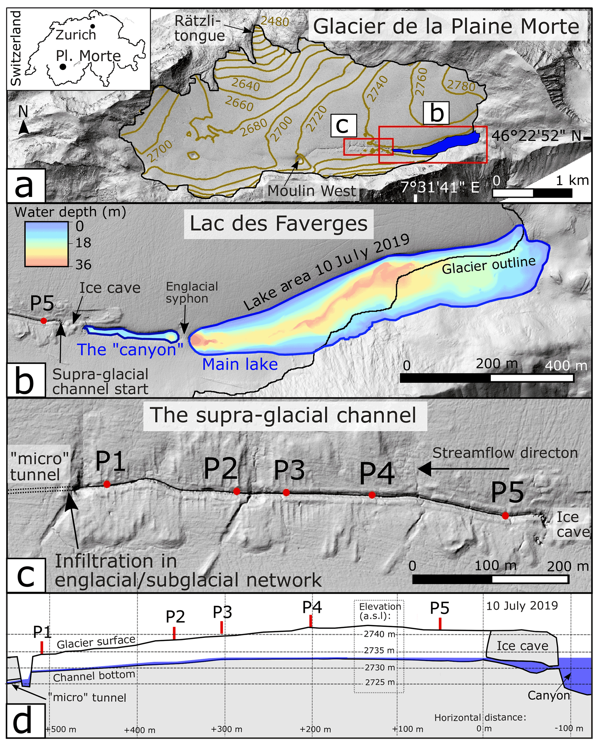
Figure 1 (a) Map of Glacier de la Plaine Morte where the ice-dammed Lac des Faverges lake is located. The lake area displayed in (b) corresponds to the maximum lake size reached on 10 July 2019 (at a lake level of 2733.15 m a.s.l). The supraglacial channel and the measurement stations P1 to P5 are presented in (c) and (d). The longitudinal profile in (d) was reconstructed from sparse elevation measurements of the glacier surface and channel bottom prior to supraglacial lake drainage; the ice cave was not mapped, and its representation is indicative only. The digital elevation model used in this figure was created from post-drainage aerial images acquired by the Swiss Federal Office of Topography on 3 September 2019 (see Sect. 3 for more information).

2.2 The 2019 GLOF mitigation plan

In spring 2019, local authorities decided to limit the maximum lake volume by constructing a supra- and englacial channel to artificially drain the lake water in order to face the increasing threat by floods due to sudden lake drainage. This channel now connects the lake outlet to a permanent large moulin located ∼ 1.3 km westwards and about 20 m lower in elevation (we will refer to this feature as the “Moulin West” in the following; see Fig. 1a). Past observations have shown that this moulin is in turn connected to the subglacial network and that this connection is often established relatively early during the melt season (Finger et al., 2013). In the middle of the channel there is a ∼ 100 m long tunnel (labelled “`micro' tunnel” in Fig. 1c), which is a remainder of the initial plan to drill a 40 cm diameter englacial tunnel, instead of a surface channel, for part of the distance (only a short section of the tunnel was completed, due to technical issues). The supraglacial channel was dug from the beginning of April until early July 2019. In a first stage, the 4–5 m deep snow cover had to be removed by snowcats. In a second stage, the solid and impermeable ice was cut and removed by an excavator. Because of these artificial interventions, the initial geometry of the channel is well known, with a width of 1 m at the bottom, a 4 to 7 m depth from the ice surface and a length of 1.3 km (see Fig. 1d). During this second stage, water from ice melt and snowmelt was present in the channel.

The lake is connected via a pre-existing ice-surface canyon and a subsequent natural ice cave to the artificial supraglacial channel (Fig. 1b). At the beginning of the canyon, where it connects to the lake, the water flows through an englacial siphon for about 30 m.

On 10 July 2019, at 11:00 CEST, the channel spillway elevation was lowered by an excavator to match the lake level and to artificially initiate the lake drainage. At that point, the spillway elevation was 2733.15 m a.s.l., corresponding to a lake volume of 1.49×10⁶ m³ ± 0.11 × 10⁶ m³ and an area of 0.127 km². The lake water ran only into the first, upper part of the channel (Fig. 1c and d) and then infiltrated the glacier through a pre-existing moulin located within the micro-tunnel. A dye injection in the channel on 26 July 2019 revealed that the lake water exited the glacier outlet after about 2 h and that there was no significant lake water accumulation within the glacier.

In the following, we limit our attention to the upper part of the channel through which the lake water flowed for 36 d in total (Fig. 1c and d). This section (termed “channel” henceforth) was located between the cave outlet and the micro-tunnel entrance, was 540 m long, and had an average slope of 0.72 %. We designed our field campaign to monitor the hydraulic and thermodynamic properties of the water flow in the channel and relate that to lake level and volume evolution.

3 Methods

Two equations are of central importance to characterize the hydraulics and thermodynamics of the lake drainage through a supraglacial channel. The first is the Darcy–Weisbach equation (Bergman et al., 2007) which relates the water flow through a channel to the hydraulic slope and to the channel cross-sectional geometry:

$$\begin{array}{}\text{(1)}& \mathit{\theta }={\displaystyle \frac{f_{\mathrm{D}}}{\mathrm{2}g}}{\displaystyle \frac{v^{\mathrm{2}}}{D_{\mathrm{H}}}},\end{array}$$

where g is the gravitational acceleration (m s⁻²), θ the hydraulic slope (dimensionless, expressed as water head drop per horizontal channel length), D_H the hydraulic diameter (m) and v the velocity averaged over the cross-section (m s⁻¹). The constant of proportionality is the Darcy–Weisbach friction factor f_D.

The second equation characterizes the thermodynamics and relates the channel incision rate m (m s⁻¹) to heat flux q (W m⁻²), where the latter can be related to the temperature difference between water and ice ΔT (K) via the dimensionless Nusselt number Nu:

$$\begin{array}{}\text{(2)}& m={\displaystyle \frac{q}{{\mathit{\rho }}_{\mathrm{i}}{L}_{\mathrm{f}}}}={\displaystyle \frac{\mathrm{1}}{{\mathit{\rho }}_{\mathrm{i}}{L}_{\mathrm{f}}}}{\displaystyle \frac{k_{\mathrm{w}}\mathit{Nu}\mathrm{\Delta }T}{\mathit{\lambda }}}.\end{array}$$

Here, k_w is the thermal conductivity of water (W m⁻¹ K⁻¹), ρ_i is the ice density (kg m⁻³), L_f is the latent heat of fusion (J kg⁻¹) and λ (m) is the length scale over which the turbulent heat transfer occurs (Bergman et al., 2007). Note that Nu is not a constant but increases with discharge and that the equations contain both physical constants (Table 1) and factors (Table 2) depending on the geometry (θ, D_H), the hydraulics (v, D_H, θ) or the thermodynamics (T_w). We will mirror this distinction in the description of the field measurements and the data processing.

In the following, we will describe our approach to obtaining all terms of those two equations, in particular by determining their dimensionless parameters f_D and Nu, with our field measurements and their suitable processing steps.

3.1 Field measurements

3.1.1 Topography

The topography of the lake and channel is necessary to characterize the geometry of the channel, to determine the watershed contribution to lake filling and to obtain the lake bathymetry in order to relate volume changes to lake surface elevation changes. To do so, we use digital elevation models (DEMs) from the Swiss Federal Office of Topography (swisstopo). These were derived by using stereophotogrammetry, aerotriangulation, ground control points and ADS100 image strips (ground sampling distance of ∼ 0.1 m) acquired during flights commissioned by the Swiss Federal Office for the Environment on 28 August 2018 and 3 September 2019 when the lake was empty (see “Code and data availability” section for references). The lake volume for the years 2012 to 2017 was also calculated using swisstopo DEMs. The theoretical nominal error in the swisstopo DEMs is 2 m but is likely to be lower in the present situation with good ground contrast. The main uncertainty in our estimate of lake volume is the poorly constrained ice-surface melt occurring in the lake basin between late August 2018 (date of DEM acquisition) and July 2019. This results in bare-ice melting in autumn 2018 and in bare-ice melting due to heat transfer from water to glacier ice before the lake drainage. Since these melt processes are not quantified in the lake basin, we constrained the lake volume using DEMs from August 2018 (1.38×10⁶ m³) and September 2019 (1.59×10⁶ m³) as a lower and upper bound, respectively. We determine the volume to be the average of the two bounds, i.e. 1.49×10⁶ m${}^{\mathrm{3}}\pm \mathrm{0.11}\times {\mathrm{10}}^{\mathrm{6}}$ m³. Note, for the subsequent calculation of lake outflow, the bathymetry of the lake is required. For this, we use the 2018 DEM because ice melt between 28 August 2018 and 10 July 2019 is expected to be significantly smaller than between 10 July 2019 and 3 September 2019.

3.1.2 Water pressure, temperature and conductivity in the channel

Most measurements were conducted at five locations (called “stations”) along the channel, named P1 to P5 (Fig. 1c and d). Stations P1 and P2 were marked with stakes drilled into the ice at the edge of the channel. At stations P3, P4 and P5 a cross-beam was installed between stakes drilled on either side of the channel. Coordinates and elevation of the stations' stakes were measured by a differential global positioning system (GPS) with a vertical accuracy of ±0.02 m.

At four stations (P1, P2, P3 and P5), autonomous and time-synchronized data loggers (DCX-22-CTD by Keller AG für Druckmesstechnik) were installed to continuously record water pressure, temperature and conductivity. The logging interval was set to 1 s during tracer experiments and to 30 s otherwise. The accuracy of temperature measurements is ± 0.1 ^∘C at stations P1 and P2 and ± 0.05 ^∘C at stations P3 and P5. We however note that this is a point measurement of the temperature with the sensor located at the floor of the channel and that the bulk water temperature is therefore likely higher. The accuracy of the pressure measurements corresponds to a water column uncertainty of 0.005 m. The accuracy of conductivity measurements is 5 × 10⁻⁵ S m⁻¹ over the range 0 to 0.2 S m⁻¹, which covered all the observations.

3.1.3 Channel geometry

At the stations, channel bottom elevation was measured using measuring tape either by lowering it from the top to the channel bottom or by abseiling with it into the channel. These measurements provide a longitudinal (i.e along the streamflow direction) channel-elevation profile and were performed 11 times during the lake drainage. Estimated uncertainties are typically 0.1 to 0.5 m in elevation and 1 m in horizontal position. The best accuracy in elevation was obtained for cross-beam stations (0.1 m). Channel width at the water flow surface was measured only infrequently at P3 and P5 due to complex accessibility, with an uncertainty of typically 0.1 m.

A higher temporal resolution of channel incision was obtained by measuring the clear diurnal melt imprints left on the channel walls at P4 and P5 between 16 and 30 July 2019 (Fig. 4). We assume that the difference in elevation between two imprints represents the daily rate of channel floor erosion. This interpretation is supported by the observation that there were 14 marks over the 14 d observation period. We suppose that the more deeply incised sections of the melt imprints form during the afternoon, when relatively high water temperature and discharge yield to significant melt on the channel walls. Conversely, a decreasing discharge and water stage during the night yields to less sideway melt on the wall section which then emerges from the water, thus producing the less deeply incised sections of the melt imprints. We thus refer to these marks as daily water level cuts. Note that the channel geometry measurements described above give the temporal evolution of the channel and thus the incision rates.

3.1.4 Hydraulics

To characterize the hydraulics of the channel, we conducted measurements of discharge Q, the flow speed v, the stage h (i.e water depth) in the channel and the lake level z_lake. In our notation, the variables used for an instantaneous measurement are marked with an index i (e.g. h_i) to emphasize the difference with variables for continuous time series. Physical quantities for a spatial average between two stations are denoted with a bar (e.g. $\stackrel{\mathrm{‾}}{w}$). Channel discharge Q_i was measured using the salt dilution method (Hubbard and Glasser, 2005) at stations P1, P2 and P3. We carried out 33 salt injections on 12 different days during the campaign. Conductivity was measured at the monitored stations downstream of the salt injection location, with stations P3, P2 and P1 situated far enough downstream to ensure the required complete mixing of the tracer. Discharge can then be calculated from the conductivity measurements, as described in Sect. 3.2.2. The tracer experiments also provide information on travel time of the water between the stations equipped with conductivity sensors, and thus an average flow speed ${\stackrel{\mathrm{‾}}{v}}_i$ between stations can be calculated.

The water stage h is measured via pressure measurements, which were corrected for atmospheric pressure variations. The measurements rely on the pressure transducer sinking to the bottom of the channel. This is ensured to be the case for all presented measurements thanks to repeated visual inspection during field visits and because pressure transducers were weighted. When pressure transducers were not at the bottom of the channel, time series were noisy and close to the atmospheric pressure value, and we discarded the data.

The elevation of the lake level z_lake was measured by two pressure transducers operated by Geopraevent, with a logging interval of 10 min. The position of the transducers was not always stable, probably due to icebergs shifting them; the resulting obvious shifts in the data were manually corrected. The absolute elevation of the lake level was measured at three instances during the drainage using a differential GPS.

3.2 Data processing

3.2.1 Lake input from precipitation, snowmelt and ice melt

Water input Q_in into the lake, by snowmelt, ice melt or liquid precipitation, was substantial during the period of lake drainage but could not be directly monitored due to its non-localized nature. Instead, Q_in was estimated by using a distributed accumulation and temperature index melt model driven by daily meteorological data (Hock, 1999; Huss et al., 2015). The model has been calibrated using the seasonal mass balance data collected by the programme Glacier Monitoring in Switzerland (GLAMOS). Seasonal mass balance has been measured on Glacier de la Plaine Morte since 2009 using the direct glaciological method (GLAMOS, 2020). We applied the model from September 2018 to September 2019 with a daily resolution to the watershed of the lake and used it to estimate Q_in consisting of snowmelt from the glacierized and ice-free portion of the basin, bare-ice melt, and liquid precipitation. The distributed mass balance model (e.g. Huss et al., 2021) was driven with meteorological observations from Montana (9 km from the study site), and both melt factors as well as a precipitation correction factor have been calibrated to match seasonal mass balance observations on Plaine Morte in 2021. The location of the watershed over the gently sloping glacier ice is inaccurately known and was adjusted to match observed total lake volume on 10 July 2019 to the cumulative Q_in since the beginning of the melting season. The implicit assumption is, thus, that no water left the lake during that time span.

3.2.2 Hydraulics

The lake outflow Q_out, which may consist of both supra- and subglacial runoff, was computed from lake-level changes Δz_lake with a diurnal resolution (Δt) by considering (1) the lake surface area A_lake as a function of z_lake according to the DEM available for 28 August 2018 and (2) the recharge from melt Q_in at day d:

$$\begin{array}{}\text{(3)}& Q_{\mathrm{out},d}=Q_{\mathrm{in},d}-A_{\mathrm{lake},d}{\displaystyle \frac{\mathrm{\Delta }{z}_{\mathrm{lake},d}}{\mathrm{\Delta }t}}.\end{array}$$

Instantaneous channel discharge Q_i was determined at P3, P2 and P1 from salt traces using the following steps. First, the natural background level of conductivity at these stations was removed for each injection, and the conductivity readings were converted into salt concentration using a calibration function derived from measurements conducted in the laboratory. The function was derived by least-squares regression of conductivity readings to salt concentration, for water temperature at 0 ^∘C and for concentration covering the entire range of observations. Second, salt concentrations were integrated over the time of the tracer passage, for each injection, and converted to discharge using the tracer dilution method (e.g. Hubbard and Glasser, 2005). We aimed to obtain a continuous discharge time series Q by using the direct measurements Q_i to calibrate a stage–discharge relationship (or rating curve) at one station as follows:

$$\begin{array}{}\text{(4)}& Q=a{h}^b,\end{array}$$

where a and b are fitted parameters and h is the continuous time series of the water stage at the selected station. The stage–discharge relation was established at P3 due to the high quality of direct discharge measurements by salt dilution (see Appendix B for values), the most continuous and reliable water stage time series, and the reasonably small geometry changes in the cross-section. Least-squares fitting yielded parameters a=4.78 ± 0.95 and b=2.05 ± 0.25. The latter is in the range of literature values for natural rivers (Aydin et al., 2002, 2006). The resulting discharge was validated against 19 discharge measurements determined using salt dilution at different times and for stations not used in the calibration. This validation resulted in an root-mean-square error of 0.11 m ³ s⁻¹, which is in line with the uncertainty in Q estimated from the standard error in parameters a and b.

A data gap in the channel's water stage time series between 13 and 24 July 2019 was filled using values based on daily lake discharge calculated using Eq. (3). To do so, we make the hypothesis that the channel is the only drainage path existing for the lake water, i.e. that there is no subglacial drainage occurring during that time period.

The average hydraulic slope ${\stackrel{\mathrm{‾}}{\mathit{\theta }}}_i$ over a channel segment of length l is

$$\begin{array}{}\text{(5)}& {\stackrel{\mathrm{‾}}{\mathit{\theta }}}_i={\displaystyle \frac{\mathrm{\Delta }{p}_i}{l}},\end{array}$$

where Δp_i is the difference between two hydraulic head measurements (i.e channel bottom elevation z_i plus water stage h_i) at the beginning and at the end of the segment. We calculated ${\stackrel{\mathrm{‾}}{\mathit{\theta }}}_i$ and subsequently derived quantities only for the segment P5–P3 because uncertainties in field measurements were the lowest for this part of the channel.

The hydraulic diameter D_H is given by

$$\begin{array}{}\text{(6)}& D_{\mathrm{H}}={\displaystyle \frac{\mathrm{4}S}{P_{\mathrm{w}}}},\end{array}$$

where S (m²) is the wetted cross-sectional area and P_w (m) is the wetted perimeter. To determine the Darcy–Weisbach friction factor f_D (see Eq. 1), the hydraulic diameter over a channel segment at a given time, ${\stackrel{\mathrm{‾}}{D}}_{\mathrm{H},i}$, needs to be determined. This is obtained by Eq. (6) using ${\stackrel{\mathrm{‾}}{S}}_i$ and ${\stackrel{\mathrm{‾}}{P}}_{\mathrm{w},i}$. ${\stackrel{\mathrm{‾}}{S}}_i$ is given by dividing the discharge ${\widehat{Q}}_i$ by the velocity ${\stackrel{\mathrm{‾}}{v}}_i$, known at the times of salt dilution experiments. The channel width $\stackrel{\mathrm{‾}}{w}$ is assumed to be constant between P3 and P5 as well as constant in time, and we found a value of $\stackrel{\mathrm{‾}}{w}=\mathrm{2}\pm \mathrm{0.5}$ m. In the following, we assume a rectangular cross-section and define the mean wetted perimeter as ${\stackrel{\mathrm{‾}}{P}}_{\mathrm{w},i}=\mathrm{2}{\stackrel{\mathrm{‾}}{h}}_i+\stackrel{\mathrm{‾}}{w}$. This assumption is motivated by the initial channel shape (i.e. the shape prior to drainage) and by visual inspections that revealed a cross-sectional shape which did not evolve substantially over time.

The mean water stage ${\stackrel{\mathrm{‾}}{h}}_i$ is calculated as ${\stackrel{\mathrm{‾}}{h}}_i={\stackrel{\mathrm{‾}}{S}}_i/\stackrel{\mathrm{‾}}{w}$. Alternatively, ${\stackrel{\mathrm{‾}}{h}}_i$ can also be calculated as the mean of the water stage of two stations; both approaches lead to similar hydraulic diameters.

Finally, the friction factor f_D is calculated from Eq. (1) with ${\stackrel{\mathrm{‾}}{S}}_i$ and ${\stackrel{\mathrm{‾}}{D}}_{\mathrm{H},i}$ between P5 and P3. Note that if we were to consider the channel cross-section to be a semi-circle, we would write $D_{\mathrm{H}}=\mathrm{2}\sqrt{S_i/\mathit{\pi }}$, and f_D would be on average 11 % smaller. As an alternative to the Darcy–Weisbach friction factor, the Manning roughness law can be preferred to characterize the flow resistance (Clarke, 2003). The Manning roughness coefficient n^′ (s m${}^{-\mathrm{1}/\mathrm{3}}$) can be calculated from f_D by $f_{\mathrm{D}}=\mathrm{8}g{n^{\prime }}^{\mathrm{2}}/R_{\mathrm{H}}^{\mathrm{1}/\mathrm{3}}$, where the hydraulic radius R_H is equal to $D_{\mathrm{H}}/\mathrm{4}$.

The Reynolds number Re (dimensionless) is the ratio of inertial forces to viscous forces within a fluid and quantifies the turbulent flow. It is calculated at the single cross-section P3 using $\stackrel{\mathrm{‾}}{w}$ and both continuous discharge Q and water stage h:

$$\begin{array}{}\text{(7)}& \mathit{Re}={\displaystyle \frac{v{D}_{\mathrm{H}}}{\mathit{\nu }}}.\end{array}$$

Here, v is $Q/S$, with $S=h\stackrel{\mathrm{‾}}{w}$, whilst D_H is calculated at P3 using Eq. (6) and ν is the kinematic viscosity (m² s⁻¹).

3.2.3 Thermodynamics

The Nusselt number Nu, i.e. the unknown parameter in Eq. (2), is defined as the ratio between convective and conductive heat transfer across the water–ice interface:

$$\begin{array}{}\text{(8)}& \mathit{Nu}={\displaystyle \frac{h_{\mathrm{t}}\mathit{\lambda }}{k_{\mathrm{w}}}},\end{array}$$

where λ (m) is the length scale over which the convective heat transfer occurs, h_t is the convective heat transfer coefficient (W m⁻² K⁻¹) and k_w is the thermal conductivity of water (W m⁻¹ K⁻¹). For λ we use the typical hydraulic diameter of the channel D_H, which is often used in glaciology (Clarke, 2003; Sommers and Rajaram, 2020) and other fields (Bergman et al., 2007; Shah and London, 1978). Note that this choice of λ is different to P_w, which was used by Walder and Costa (1996) when simulating ice-dam breaches.

Since the hydraulic diameter strongly depends on the channel width in the case of a broad channel, it is relatively poorly constrained in our study. We therefore define λ as the typical, and constant, hydraulic diameter which we calculate using Eq. (6). With $\stackrel{\mathrm{‾}}{h}$ being the typical water stage observed in the channel ($\stackrel{\mathrm{‾}}{h}=\mathrm{0.5}\pm \mathrm{0.1}$ m), we obtain $P_{\mathrm{w}}=\mathrm{3}\pm \mathrm{0.54}$ m and ${\stackrel{\mathrm{‾}}{D}}_{\mathrm{H}}=\mathrm{1.30}\pm \mathrm{0.22}$ m. For comparison, the ${\stackrel{\mathrm{‾}}{D}}_{\mathrm{H},i}$ calculated above ranges between 1.0 and 1.6 m, with a mean value of 1.26 m. We then use $\mathit{\lambda }={\stackrel{\mathrm{‾}}{D}}_{\mathrm{H}}$ to obtain Nu in Eq. (8).

In glaciological applications and elsewhere, Nu is usually calculated using an empirical relation, often the Dittus–Boelter equation (e.g. Clarke, 2003; Spring and Hutter, 1981; Nye, 1976) or the Gnielinski correlation (e.g. Ancey et al., 2019). These two equations parameterize Nu using the Reynolds (Re) and Prandtl (Pr) numbers, where the latter is the ratio of the dynamic viscosity to the thermal diffusivity of water (Pr = 13.5 at 0 ^∘C; Clarke, 2003). The Dittus–Boelter equation reads

$$\begin{array}{}\text{(9)}& \mathit{Nu}=A{\mathit{Pr}}^{\mathit{\alpha }}{\mathit{Re}}^{\mathit{\beta }},\end{array}$$

where A, α and β are empirical coefficients given in the literature (Bergman et al., 2007). The Gnielinski correlation additionally uses f_D and reads

$$\begin{array}{}\text{(10)}& \mathit{Nu}={\displaystyle \frac{\frac{f_{\mathrm{D}}}{\mathrm{8}}(\mathit{Re}-\mathrm{1000})\mathit{Pr}}{\mathrm{1}+\mathrm{12.7}{\left(\frac{f_{\mathrm{D}}}{\mathrm{8}}\right)}^{\frac{\mathrm{1}}{\mathrm{2}}}({\mathit{Pr}}^{\frac{\mathrm{2}}{\mathrm{3}}}-\mathrm{1})}}.\end{array}$$

In addition to these two empirical relations, we present below two alternative methods to calculate Nu directly from our measurements (i.e. without using a parameterization). We can thus compare our findings to the above empirical equations. The first method, termed the melt-rate method, considers the melt rate and water temperature at one location as a function of time. Nu is then directly derived from Eq. (2) with the vertical melt rate m given by repeated channel floor elevation measurements and with the water temperature given by the continuous monitoring. The water temperature measurements are averaged over the time span between two channel-elevation measurements; therefore, Nu obtained by using the melt-rate method is time-averaged as well.

The second method, termed the spatial-cooling-rate method, considers the water temperature at an instance in time and its decrease as a function of distance along the channel. The water temperature T_w(x) decreases following an exponential law (e.g. Isenko et al., 2005), which can be derived from energy conservation (see Appendix A) and can be written as

$$\begin{array}{}\text{(11)}& T_{\mathrm{w}}\left(x\right)=T_{\mathrm{0}}{\mathrm{e}}^{-\frac{x}{x_{\mathrm{0}}}},\end{array}$$

where x is the distance (m) from the origin (in our case P5, the uppermost monitoring station), T₀ is the temperature at this location (^∘C) and x₀ is the e-folding length (m). Physically, x₀ is the distance over which the temperature decreases by a factor e and can be expressed in terms of Nu, Q and the wetted perimeter ${\stackrel{\mathrm{‾}}{P}}_{\mathrm{w}}$ as

$$\begin{array}{}\text{(12)}& x_{\mathrm{0}}={\displaystyle \frac{Q{c}_{\mathrm{w}}{\mathit{\rho }}_{\mathrm{w}}\mathit{\lambda }}{\mathit{Nu}{k}_{\mathrm{w}}{\stackrel{\mathrm{‾}}{P}}_{\mathrm{w}}}},\end{array}$$

where c_w is the specific heat capacity of water (J K⁻¹ kg⁻¹). We obtain x₀ from a least-squares fit of Eq. (11) to the hourly averaged temperature at stations P5, P3, P2 and P1, and, thus, Nu can be calculated.

3.2.4 Uncertainty propagation

In this study, uncertainties in field measurements come from the sensors' sensitivity and limitations of the measurement procedures. Both uncertainties are quantified and propagated through the equations by using a Monte Carlo approach (Carlson, 2020). Since this allows us to also propagate errors faithfully through non-linear functions, results are systematically presented with their standard deviation.

Table 1 Physical constants used in this work. If not specified, constant refers to the property of water at 0 ^∘C.

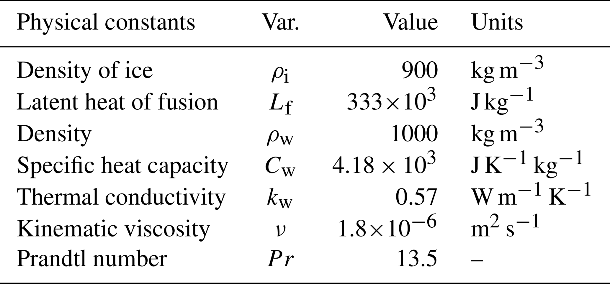
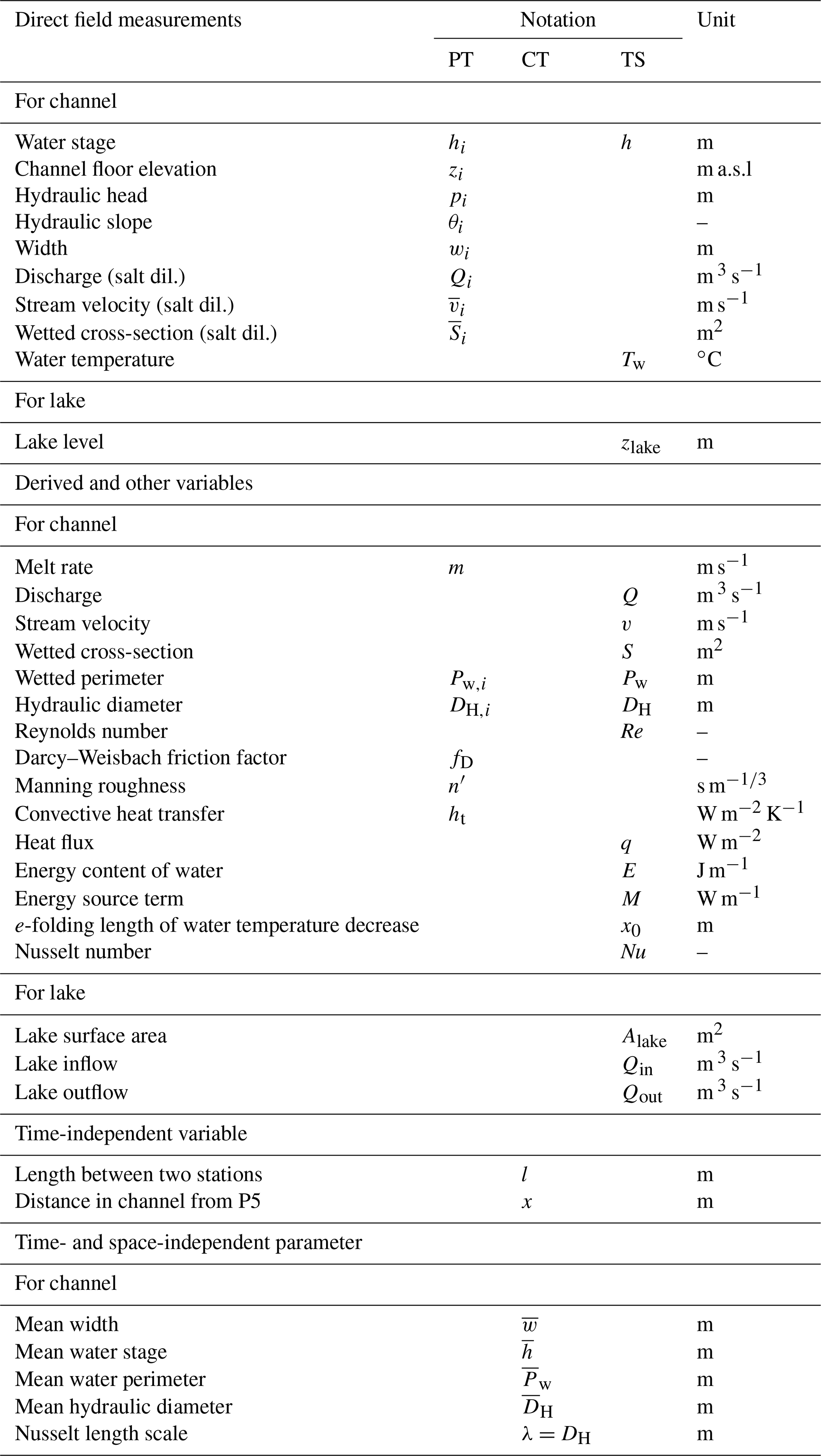
Table 2 Table of variable names. The term salt dil. stands for “salt dilution experiment technique”, and a.s.l stands for “above sea level”. Individual quantities might be available either for a point in time (PT; the index (i) means that the measurement is instantaneous) or as a time series (TS), or they might be constant through time (CT). A bar over the corresponding symbol indicates that the quantity is averaged over a given channel segment, i.e. between two stations.

4 Results

4.1 Lake drainage hydrographs 2012–2019

Figure 2 shows the temporal evolution of lake water volumes between 2012 and 2019 and hourly averaged discharge. The lake water input Q_in was only accounted for in the year 2019 since it becomes relevant to take it into account in the calculation of Q_out, due to a much smaller value of the latter compared to in previous years. The increasing trends of both maximum volume and peak discharge from 2012 to 2018 are clearly visible. The drainage onset time depends, amongst other things, on the meteorological conditions during the lake-filling phase. In warmer years, the date of complete filling of the lake basin occurs earlier. Also, an early depletion of the winter snow cover is likely to be linked with an early development of the subglacial drainage system, which in turn favours subglacial lake drainage (GLAMOS, 2018). Since 2014, the lake volume has systematically reached more than 2×10⁶ m³, and the subglacial release of the total lake water occurred within a few days, except for in 2015 when the water drained through a supraglacial channel into a nearby moulin for about 2 weeks.

The 2019 lake drainage pattern is drastically different from in previous years due to the artificial intervention. We distinguish four different phases. The first phase (Phase I) is from 10 July to 1 August 2019, when approximately half of the lake emptied through the supraglacial channel. Phase II is from 2 to 15 August 2019, when the lake level remained roughly constant but lake water was still running in the channel. Phase III is from 15 to 21 August 2019, when lake water stopped running in the channel and the lake level remained constant or slightly increased. Phase IV is from 22 to 27 August 2019, when the second half of the lake volume emptied subglacially, which is similar to the natural drainage mechanism of previous years. Note that the discharge peak of 3.5 m³ s⁻¹ was much lower compared to in other years, e.g. over 20 times lower than in 2018 (Fig. 2). In this regard, the technical intervention was very successful.

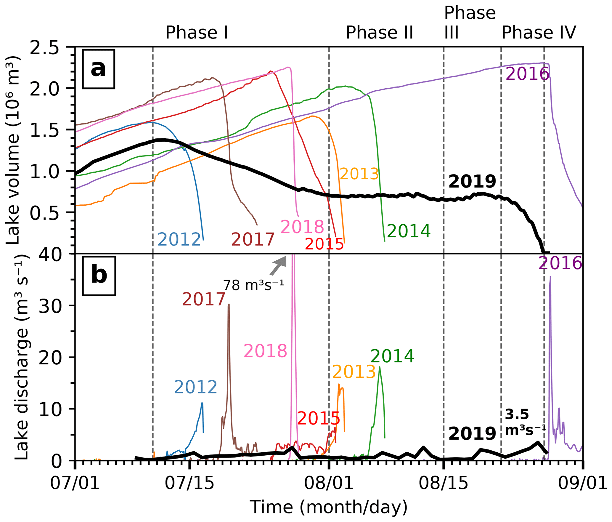
Figure 2 Lake volume (a) and lake discharge (b) during summer from 2012 to 2019. The year 2019 is represented by a black and thicker line. Discharge is shown as hourly averages for 2012 to 2018 and daily averages for 2019. Note that the 2018 discharge peak (78 m³ s⁻¹) is beyond the plotted range.

4.2 Channel geometry

The channel bottom elevation and its evolution with time at five locations along the channel is presented in Fig. 3. The incision shows a uniform spatial pattern and is about 8 m during the supraglacial drainage (Phase I and II, 10 July–15 August 2019). Note that the channel slope was not uniform prior to the drainage onset (Fig. 1d) and that it remained relatively constant after natural adjustments during the first days of drainage. The low slope at the channel segment P5–P3 leads to uniform streamflow, which allowed the formation of clear daily water level cuts (Fig. 4). In contrast, the higher slope between P2 and P1 led to more turbulent water flow and subsequent formation of step pools (e.g. Vatne and Irvine-Fynn, 2016). Note that meandering (Karlstrom et al., 2013) did not occur, and, thus, the channel length stayed constant.

Widening is substantial only at P5 where channel width increased from 1 m on 10 July to 3 ± 0.1 m on 8 August 2019. Further downstream, e.g. at P4, the widening is minor (Fig. 4). Overall, the channel geometry was mainly driven by vertical incision rather than lateral melting.

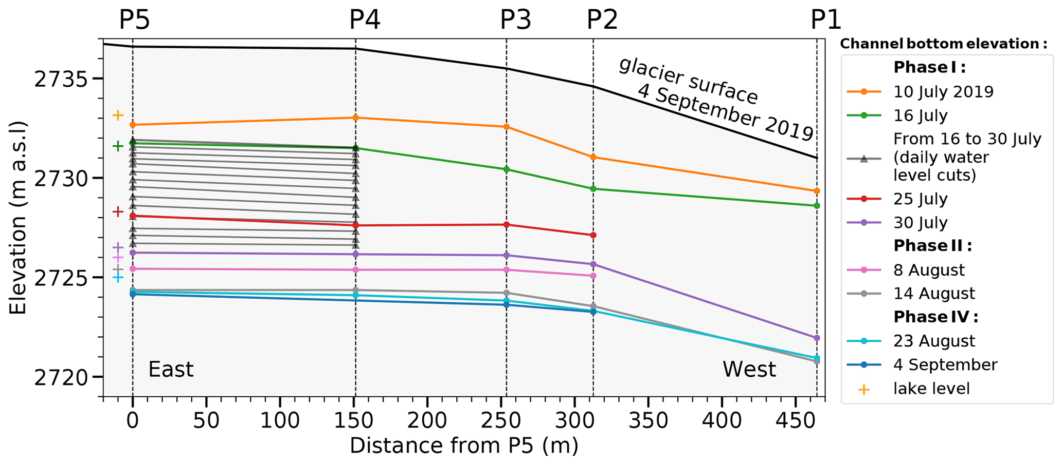
Figure 3 Channel bottom elevation at P5, P4, P3, P2 and P1 during the lake drainage (locations are presented in Fig. 1). The colour-coded crosses indicate the lake level at the corresponding time. Note that the actual lake was located further east than P5. Distances between stations are taken along the channel flow path.

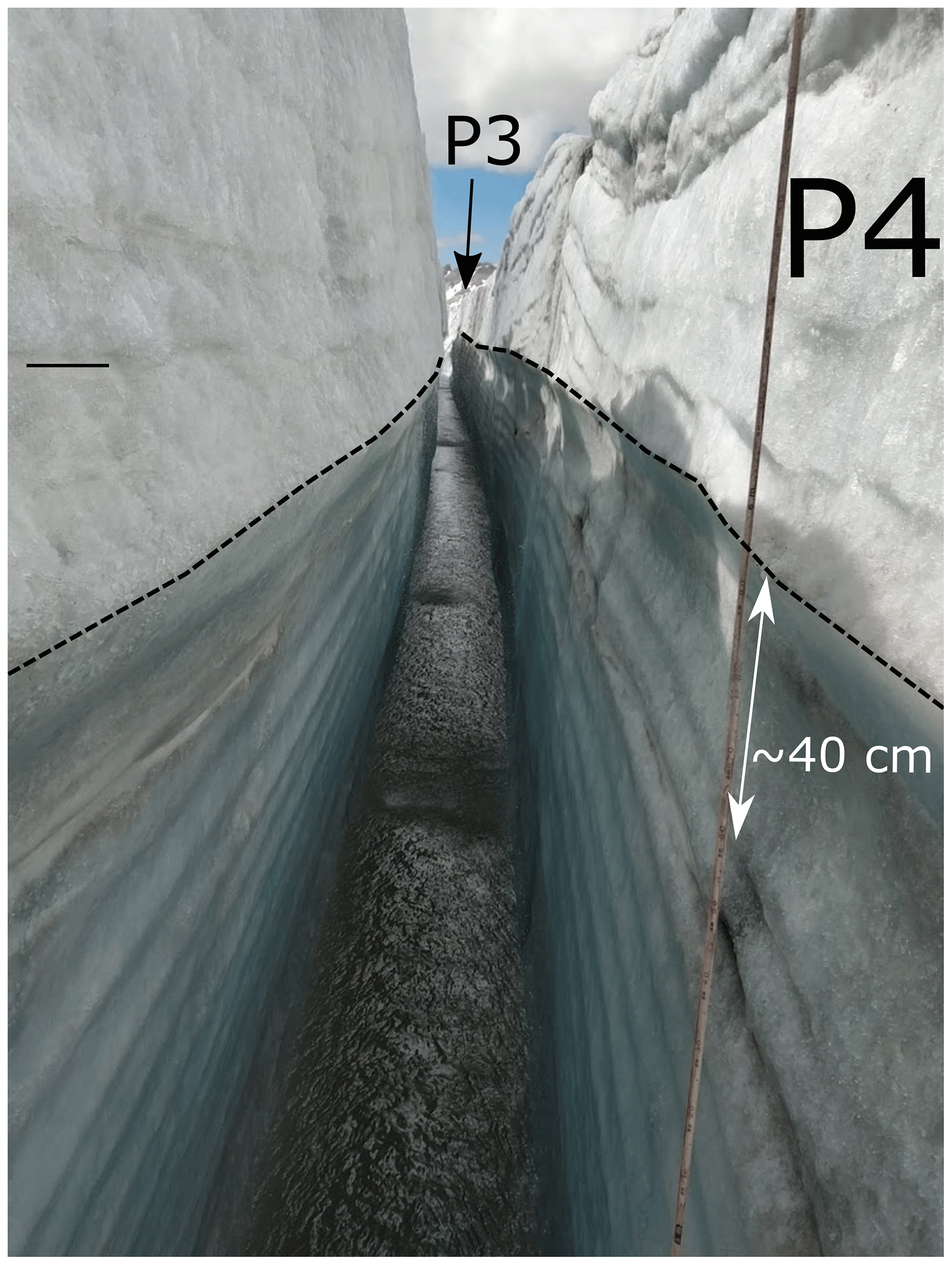
Figure 4 Photo from within the supraglacial channel from P4 towards P3. The dashed line represents the highest water stage in the channel (10 July 2019) prior to the supraglacial lake drainage start and prior to the onset of the channel bottom incision. Daily water level cuts are clearly visible on both sides. The picture was taken on 30 July 2019.

4.3 Channel hydraulics

The water stage (Fig. 5) and the hydraulic slope determine the water discharge. Water stage measurements were challenging during the first days of the supraglacial drainage (i.e. 10 July 2019, beginning of Phase I) since the excavator used to deepen the channel spillway left irregular traces on the channel bottom. Nevertheless, probe measurements (at P5, P4, P3, P2 and P1) together with water pressure sensors (at P5, P3, P2 and P1 only) reveal that the water stage on 10 July 2019 was around 1 m at P5, 0.4 m at P4 (which was close to the spillway location) and 0.3–0.5 m for the other stations. The water stage stabilized at 0.6 m after a few days of drainage (Phase I) at P5 and at around 0.4–0.5 m at the other stations. Daily fluctuations were typically 0.1 m due to the daily melting cycle influencing the lake input. At P1, measurements were soon no longer feasible because of the formation of step pools. The water stage slowly decreased to a value of 0.1–0.2 m uniformly over the channel during Phase III and Phase IV, when lake water no longer drained through the channel.

Figure 5 Hourly time series of the water stage at P5 (dashed black line) and P3 (blue line) from continuous pressure measurements. Direct observations (and associated standard errors) from field visits are marked by black diamonds and blue dots for P5 and P3, respectively. Part of the discrepancies between direct field observations and the continuous water stage from pressure sensors can be explained by the probing not always being made at the exact location of the sensors.

Figure 6 presents time series of water temperature, channel discharge and channel bottom elevation at station P3, along with the lake level. Data gaps in discharge and temperature time series are due to disruptions of logging. The daily mean discharge time series between 13 and 24 July 2019 has been calculated using lake-level change and modelled lake inflow (see Sect. 3.2.2). The peak in channel discharge was reached on 14 July 2019 (Phase I), with a daily average of 1.7 m³ s⁻¹. The good agreement between the different direct discharge measurements (${\widehat{Q}}_i$) and the continuous discharge at P3 indicates that the stage–discharge relationship is valid over the entire drainage duration. The decoupling between Q at P3 and Q_out during Phase III and IV (Fig. 6b) is because the lake no longer drained through the channel at that stage. The temperature and discharge signal of the lake water is clearly visible in the channel until 14 August 2019. This is in contrast with the temperature signal from the glacier's daily melt pattern from 23 August to 4 September 2019 (water temperature close to 0 ^∘C at night), when the lake was no longer draining through the channel (beginning of Phase III).

The stable mode of drainage during Phase I is corroborated by the observation that the distance between daily water level cuts in the channel (indicative of channel floor erosion; see Sect. 3.1.3) corresponds to the rate at which the lake level lowers (Fig. 6). At P5, this distance varies between 30 and 60 cm d⁻¹ during the second half of July 2019 and drops on average to 12 cm d⁻¹ for the first half of August 2019.

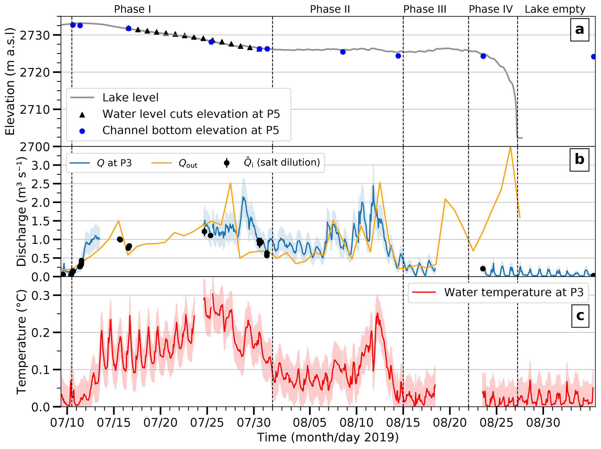
Figure 6 (a) Lake-level elevation (continuous curve), channel bottom elevation (blue dots) and water level cut elevations (black dots) at P5. (b) Hourly channel discharge at P3 (Q), direct discharge measurement by salt dilution averaged over all stations (${\stackrel{\mathrm{‾}}{Q}}_i$) and lake discharge from elevation change (Q_out). (c) Water temperature at P3. The four distinct lake drainage phases are delimited by the dashed line and explained in the main text (Sect. 4.1). Standard uncertainties for hourly discharge and temperature are shown with light bands.

The streamflow in the channel is highly turbulent during supraglacial drainage. The Reynolds number fluctuates with discharge and is between 2.5 × 10⁵ and 1.5 × 10⁶ (Phase I and II). Note that the transition between laminar flow in the lake and turbulent flow somewhere at the channel entrance is further upstream than P5 (the location is not known exactly).

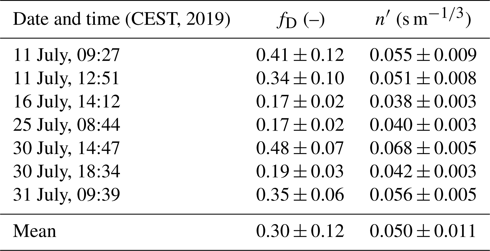
The Darcy–Weisbach friction factor was calculated for the channel segment between P5 and P3, where accurate calculation of ${\stackrel{\mathrm{‾}}{D}}_{\mathrm{H}}$ and thus ${\stackrel{\mathrm{‾}}{P}}_{\mathrm{w}}$ was possible. The time series of the inferred friction factor is presented in Table 3.

Table 3 The Darcy–Weisbach friction factor f_D and Manning roughness n^′ with associated standard deviation in the channel segment between stations P5 and P3. All measurements were performed during Phase I of the drainage when salt dilution experiments were conducted (see Fig. 6).

4.4 Thermodynamics

Water temperature, measured continuously at P5, P3, P2 and P1, shows an exponential decrease along the channel (Fig. 7) and exhibits daily fluctuations (Fig. 6, e.g. ±0.1 ^∘C during Phase I). The relation given in Eq. (11) is fitted to these temperature observations. Note that the pattern was similar whenever lake water was flowing through the channel.

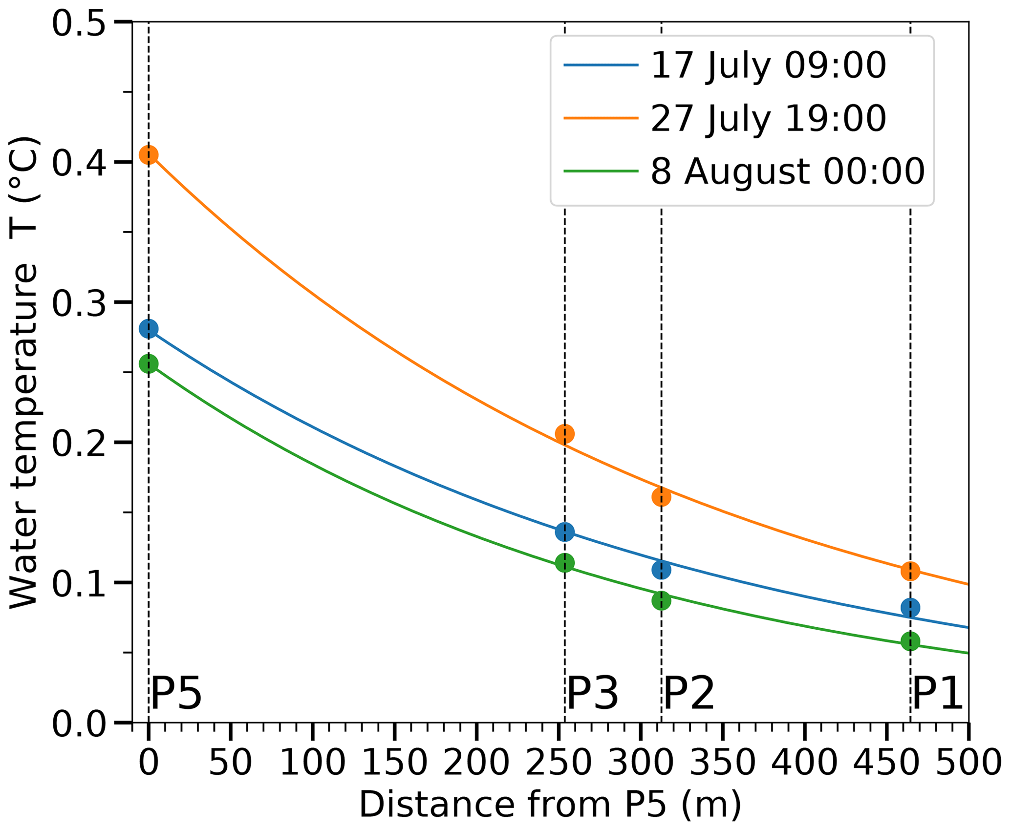
Figure 7 Temperature decrease along the channel flow path at three different times (CEST). Dots are observations; lines correspond to the fitted exponential law according to Eq. (11).

Figure 8 presents time series of the Nusselt number Nu calculated from our measurements according to the melt-rate method (Eq. 2) and the spatial-cooling-rate method (Eq. 12), as well as from the empirical Dittus–Boelter equation (Eq. 9) and the Gnielinski correlation (Eq. 10). For the Dittus–Boelter equation we use coefficients A, α and β from previous studies (Table 4); for the Gnielinski correlation, we use the mean friction factor f_D=0.3 (Table 3). The heat transfer is dominated by convection, with typical Nu values on the order of 10⁴. The results from the melt-rate and spatial-cooling-rate methods are in good agreement, except for the period 11–16 July 2019 (beginning of Phase I). For this period, the higher Nu values obtained by the melt-rate method compared to the spatial-cooling-rate method could be explained by the very high melt rate at P3 (see Fig. 3).

Our values for Nu are significantly higher than the ones derived from the Dittus–Boelter equation using standard coefficients (e.g. Clarke, 2003). We note, however, that the coefficients used by Lunardini et al. (1986) and Vincent et al. (2010) result in Nu values that lie at the lower and upper edge, respectively, of the uncertainty range of our Nu values. Conversely, the Gnielinski correlation produces values of Nu that are significantly higher than our results, as well as the ones obtained by the alternative methods.

(e.g. Clarke, 2003)Lunardini et al. (1986)Vincent et al. (2010b)

Table 4 Dimensionless coefficients of the Dittus–Boelter equation (Eq. 9) from various studies, including this one (see Sect. 3.2.3).

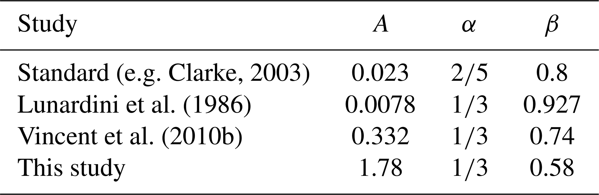
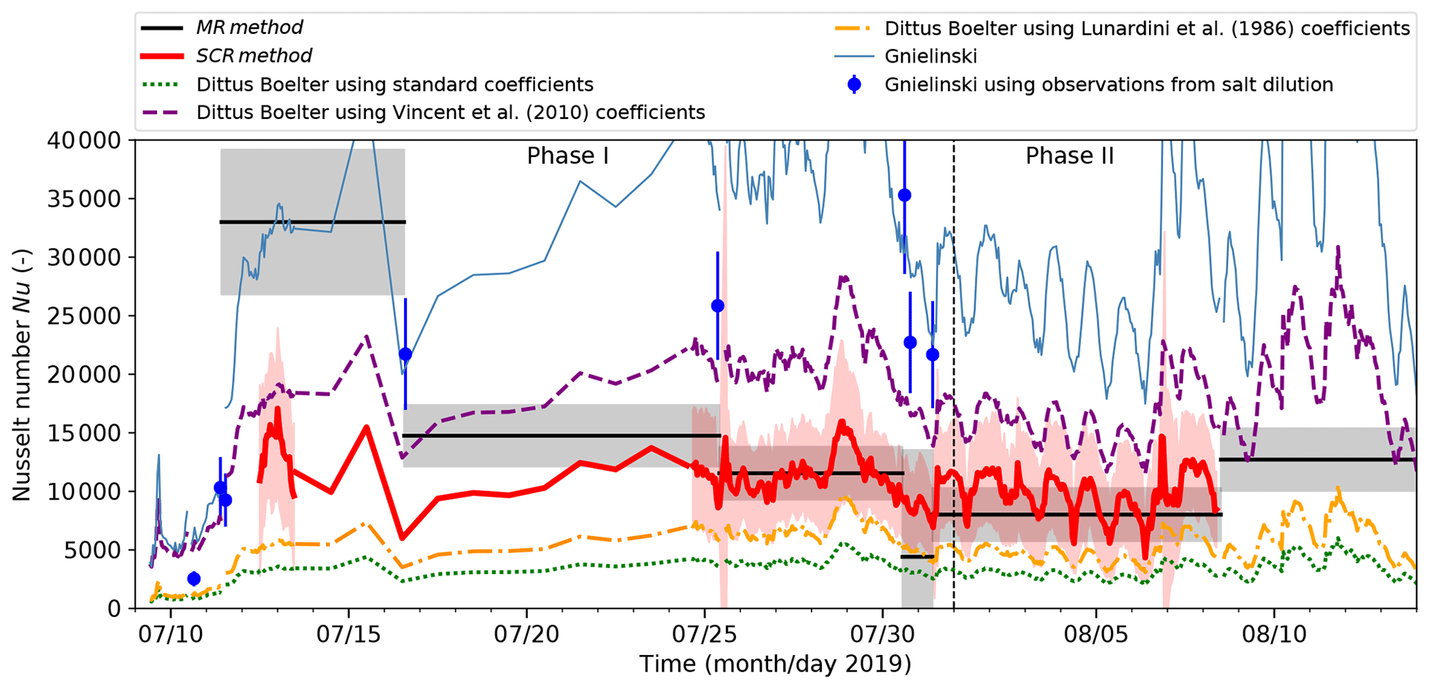
Figure 8 Nusselt number Nu at P3 computed using two different approaches and several empirical relations. MR method refers to the melt-rate method (Eq. 2), and SCR method refers to the spatial-cooling-rate method (Eq. 12). The Dittus–Boelter equation and the Gnielinski correlation are presented in Eqs. (9) and (10), respectively. For the sake of readability, the standard deviation (band around the mean values) is only displayed for the values derived from our measurements. The vertical dashed line separates Phase I and II of the lake drainage.

The Nusselt number Nu is dependent on the Reynolds number Re via turbulent mixing. Figure 9a shows the relation between Nu and Re as determined by our field measurements, along with the previously used parameterizations for Nu. It is noteworthy that our results show a less pronounced dependence of Nu on Re than other assessments. Indeed, fitting the Dittus–Boelter equation (coefficients A and β, Eq. 9) to our data yields an exponent of β=0.58, which is low compared to exponents of between 0.75 and 0.93 found by Clarke (2003), Lunardini et al. (1986) and Vincent et al. (2010b) (Table 4).

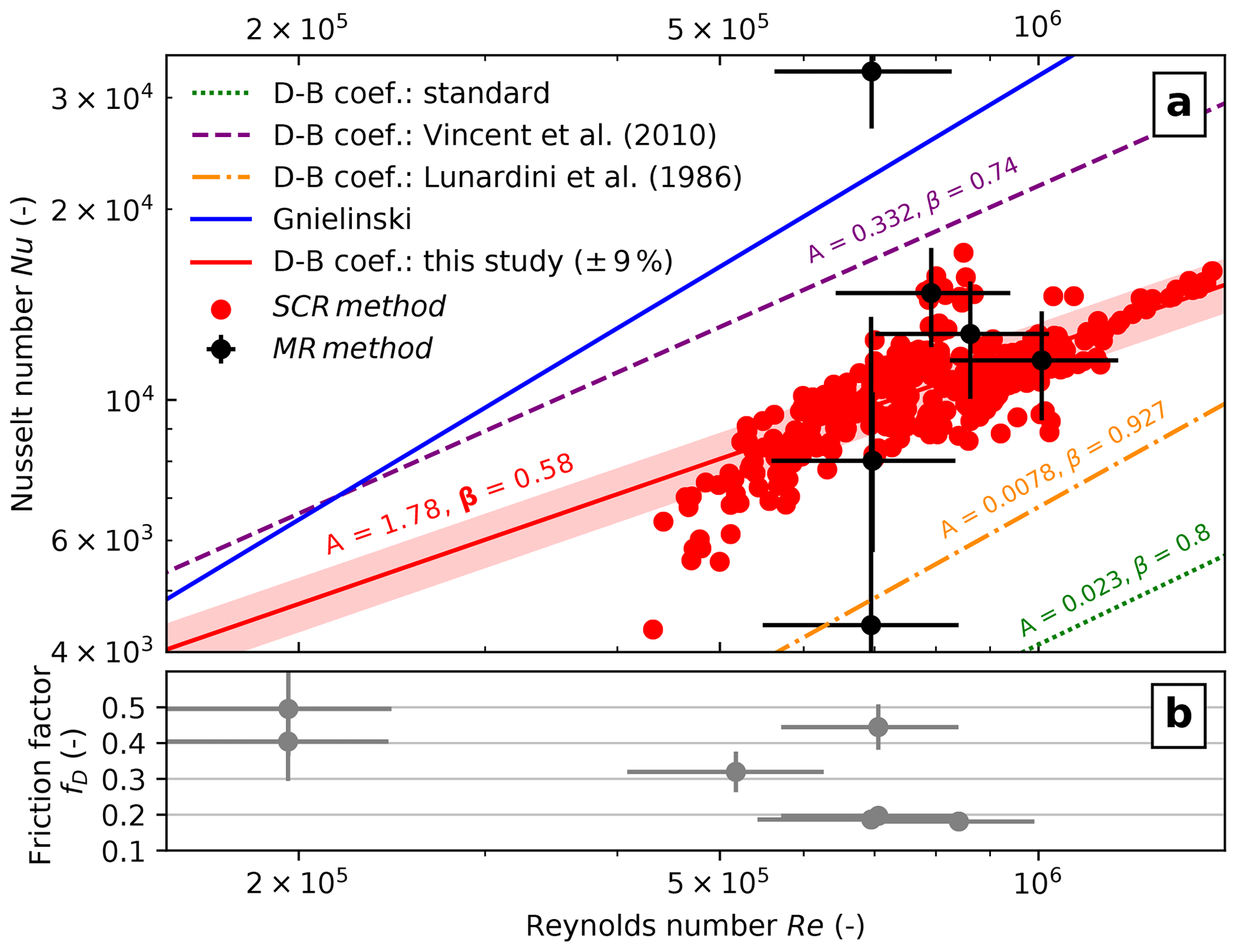
Figure 9 The Nusselt number (a) and friction factor (b) against the Reynolds number (Eq. 7). Note that all quantities are dimensionless. The Nusselt number from our observations is calculated using the melt-rate method at P3 (Eq. 2) and the spatial-cooling-rate method (Eq. 12). The band shows the mean relative error of 9 %. The Nusselt number is also calculated from the Dittus–Boelter equation Eq. (9) using coefficients (named “D–B coef.” in the legend) from other studies (see Table 4) and the Gnielinski correlation (Eq. 10).

5 Discussion

We collected an extensive dataset of a supraglacial lake drainage through a channel and characterize its hydraulics and thermodynamics. We derive key parameters, namely the factors of hydraulic friction and heat transfer. In the following, we discuss the implications of our findings for future studies and for hazard mitigation measures.

5.1 Reconstruction of the lake drainage during Phase I–IV

The four phases of the lake drainage are interpreted as follows: Phase I is characterized by stable supraglacial lake drainage, i.e. the lake drawdown is controlled by the rate of vertical channel incision. There is a significant difference between the computed lake outflow Q_out and the channel discharge Q at P3 during the sub-period 26 July to 30 July 2019 (Fig. 6b), coinciding with strong rain that ended a heat wave which started on 20 July 2019.

During Phase II, the lake level remained constant (Fig. 6a), but the lake water was still running in the channel as evidenced by the relatively warm water (Fig. 6c). This is indicative of the outflow of the lake-channel system behaving like a non-erosive spillway: the channel only received the water from snowmelt and ice melt, which spilled above a constant elevation. The exact location of the spillway is unknown: it could be located either in the englacial siphon between the main lake and the canyon or in the ice cave (Fig. 1) although visual inspection gave no evidence for the latter. Phase III is characterized by the stopping of the supraglacial drainage around 15 August 2019. It is likely that the lake surface became too small, such that the lake drawdown became higher than the channel incision. This is especially likely if the channel was disconnected from the main lake by the spillway between the canyon and the main lake or in the case of subglacial leaks. Although no sensors were installed in the channel from 19 to 23 August 2019, the channel incision between 14 and 23 August 2019 was negligible (Fig. 3). This indicates that the peak in Q_out on 19 August 2019 was due to subglacial rather than supraglacial drainage.

During Phase IV, the lake emptied subglacially, with no influence from the supraglacial channel. The triggering mechanism is presumably similar to in previous years. Lindner et al. (2020) showed, for example, that the drainage in 2016 was initiated by hydrofracturing.

5.2 Hydraulics

We calculated the hydraulic friction factor f_D of the channel at several instances during Phase I (Table 3), when the necessary salt dilution measurements were available. Values for f_D range from 0.17 to 0.48, corresponding to a Manning roughness n^′ of 0.038 to 0.068 s m${}^{-\mathrm{1}/\mathrm{3}}$. These values are similar to the ones of Mernild et al. (2006), who inferred n^′ to be between 0.036 and 0.058 s m${}^{-\mathrm{1}/\mathrm{3}}$ in supraglacial streams on the Greenland Ice Sheet. Similar observations of Gleason et al. (2016) revealed strong variability in n^′ in time and space, ranging from 0.009 to 0.154 s m${}^{-\mathrm{1}/\mathrm{3}}$ with a mean value of 0.035 ± 0.027 s m${}^{-\mathrm{1}/\mathrm{3}}$, similar to ours. The lower end of their range corresponds to a smooth channel, whereas the upper end cannot be explained by ice-channel roughness alone and is an indication not only of slush ice being present in the channel but also of the influence of form friction (as opposed to skin friction) in a complex three-dimensional channel geometry.

Why the friction factors vary so much is unclear from our observations. For instance, there is no correlation with the Reynolds number (Fig. 9b). Previous studies have already highlighted the need to better quantify the hydraulics of englacial channels (e.g. Clarke, 2003; Gleason et al., 2016) and the need for additional in situ observations to better constrain the parameters that control discharge (e.g. Kingslake et al., 2015; Smith et al., 2015). Our work provides a range of accurate, field-based friction factors for a supraglacial stream at different times during a lake drainage and shows its variability. However, the large range of friction factor values reported here and in other studies suggests that using a constant value in modelling studies could be inappropriate. Instead, we suggest that modelling studies should treat f_D as a stochastic variable (e.g. Brinkerhoff et al., 2021; Irarrazaval et al., 2021), i.e. that they should use a range of values as opposed to a single one.

5.3 Thermodynamics

In general, the supraglacial drainage of an ice-dammed lake progresses via the incision of the channel by melt. The incision rate determines whether the lake drains gradually, i.e. with an approximately constant discharge over time, or unstably, i.e. with a progressively increasing discharge (Raymond and Nolan, 2000).

To characterize channel incision, the heat transfer between the advected lake water and the ice channel walls needs to be quantified. This heat transfer is captured by the Nusselt number Nu, which was derived from measurements in this study. Our results (Figs. 8 and 9) are in between the predictions of the Dittus–Boelter equation (Eq. 9) using the parameters from Vincent et al. (2010), which are higher than our values, and those of Lunardini et al. (1986), which are lower than our values. This suggests that using the parameterizations of these two studies, which have a cryospheric context as well, gives an interval of Nusselt numbers to consider. Again, as with the hydraulic friction factor, the large range of plausible Nusselt numbers means that it should be a stochastic parameter in modelling studies.

The cause of the discrepancy between the exponent of the Reynolds number in the Dittus–Boelter equation determined in our study (β=0.58) and others (β between 0.75 and 0.93, Table 4, Fig. 9a) is not clear. Our water temperature measurements were conducted using CTD sensors which sunk to the channel bottom. Their close proximity to the ice means that they might have measured a temperature below the bulk water temperature, which would lead to an overestimation of Nu using the melt-rate method. Conversely, the results of the spatial-cooling-rate method would likely be less impacted as the temperature e-folding length should not depend on the location of the sensors. Future studies should put an emphasis on accurate water temperature measurements, for instance by using fibre optics methods as in Karlstrom et al. (2014), paying attention to accurately estimating the bulk water temperature.

Longitudinal temperature profiles of supraglacial channels have been studied in both the field and the laboratory but only by one study so far (Isenko et al., 2005). Water temperature decreases exponentially with distance, which is the basis of estimating Nu in our spatial-cooling-rate method (Eq. 12). This method is useful because it is easier to implement and allows a higher sampling rate than the melt-rate method (Eq. 2) since it only requires temperature measurements and not the more challenging channel incision rate measurements, as were used in other studies (e.g. Vincent et al., 2010). If the melt-rate method is chosen, direct measurements of channel incision are needed, and we support the idea of Raymond and Nolan (2000) that daily water level cuts can be used to conduct those measurements a posteriori (Fig. 4).

Besides the incision rate, the channel aspect ratio plays a major role in the drainage stability of a supraglacial lake: for a given stage, a wider channel has a bigger discharge capacity than a narrower channel and will consequently contribute to stabilizing the drainage by accelerating the lake-level drawdown (Raymond and Nolan, 2000, their Eq. 8). Channel width was considered constant in the present field study and was used to calculate the hydraulic diameter and consequently all parameters which are derived from it. The large uncertainties we applied to the width take into account a potential change in width, and the estimated parameters take this fully into account. Moreover, our stage–discharge relation at P3 seems to work well despite a slight widening at that location.

The channel aspect ratio was considered by Jarosch and Gudmundsson (2012), who suggest that this ratio is determined by the melt-rate dependence on water depth: if the melt rate is independent of water depth, a very broad channel forms, whereas if it scales linearly, a nearly semi-circular channel forms. To our knowledge, there is no theoretical work available for how melt rates are distributed over the channel perimeter, but extending the study of Sommers and Rajaram (2020) could shed light on this issue. Future field-based studies could try to quantify the channel aspect ratio, as it would give indications of both lake drainage stability and melt-rate distribution along the channel perimeter.

5.4 Hazard mitigation

The maximum lake volume of 1.49×10⁶ m³ ± 0.11×10⁶ m³ reached in 2019 was limited by the constructed supraglacial channel to about two-thirds of its potential volume, and half of the lake water (∼ 0.7 × 10⁶ m³) drained, stably, through the channel once the lake overspilled into it. In this sense, the hazard mitigation of Lac des Faverges was very successful; however construction costs were considerable at CHF 1.7 million. Still, construction costs were lower than the damage costs of CHF 2.5 million in 2018 alone. The relatively small volume of remaining water later drained subglacially during an outburst event (Fig. 2). The peak discharge was only ∼ 3.5 m³ s⁻¹ and thus far lower than the ∼ 80 m³ s⁻¹ recorded in 2018.

The intervention at Lac des Faverges thus indicates that a channel dug at the glacier surface prior to the lake filling can successfully limit the maximum lake volume and thus the hazard potential. Indeed, partially or fully filled lakes have been successfully drained in the past via such channels (e.g. Vincent et al., 2010), although not at the scale of the present artificial intervention. Nonetheless, surface lake drainages also have considerable hazard potential (e.g. Ancey et al., 2019; Walder and Costa, 1996), and therefore the prediction of whether a surface drainage proceeds stably or unstably is critical for hazard assessments. Raymond and Nolan (2000) proposed a criterion based on lake area and temperature (their Eq. 8). The area and temperature of Lac des Faverges respected this stability criterion when the drainage initiated in 2019 but only barely. However, the past surface drainage of 2015 (Fig. 2), which drained stably through a shorter channel (about 400 m), suggests that the 2019 drainage was well within the stable regime; refining this criterion would help improve future hazard assessments.

The artificial channel remained active throughout the summer of 2020, and it was effective in limiting the lake volume and thus the hazard emerging from it. In terms of operations, the substantial amounts of winter snow blown into the channel proved to be challenging as they formed an intermediate blockage. In early August 2020, the winter snow was partially removed by an excavator, and the remaining snow blockage was eroded in a slush-flow-like event, after which the lake drained partially through the supraglacial channel (i.e. corresponding to Phase I in Fig. 6) and partially subglacially (i.e. corresponding to Phase IV in Fig. 6). Since the slush-flow-like event was relatively difficult to control, additional artificial measures were taken for 2021. These aimed at activating the channel's water flow underneath the extensive snow cover that rebuilds during winter. However, in 2021 the lake drained subglacially when only half full and before lake water could flow through the channel; the lake outlet was situated in the “canyon” region (Fig. 1b). The drainage occurred in late July 2021 which was early relative to the still extensive snow cover and to the low filling level.

6 Conclusions

In 2019, the ice-dammed Lac des Faverges, located on Glacier de la Plaine Morte in the Swiss Alps, partially drained through an artificial supraglacial channel, constructed in order to mitigate the hazard posed by this lake. This unique setting was used to acquire a comprehensive dataset describing the evolution of the lake level, channel discharge, channel incision and channel-water temperature during drainage. It is probably one of the most comprehensive of such datasets currently available.

The field measurements were used to characterize the hydraulics and thermodynamics of the supraglacial channel, quantifying, among other parameters, the friction factor and the Nusselt number. The observed Darcy–Weisbach friction factors range between 0.17 and 0.48, with a mean value of 0.30, which is close to what other studies have found and to what modelling studies have used so far. However, the large spread found in our study suggests considering the friction factor a stochastic variable, instead of a constant.

The heat transfer between water and channel wall, responsible for channel incision and quantified by the Nusselt number, was determined using two distinct methods: the melt-rate method and the spatial-cooling-rate method. The results of the two methods agree, but as with the hydraulic friction factor, a large spread is found, indicating that the Nusselt number should also be treated as a stochastic variable in modelling studies. The Nusselt numbers derived from the often-used empirical Dittus–Boelter equation are significantly different to ours. More precisely, the dependence of the Nusselt number on the Reynolds number is less pronounced than previously reported (e.g. Clarke, 2003; Lunardini et al., 1986; Vincent et al., 2010) or in the commonly used empirical Gnielinski correlation. We identify the heat transfer rate as one of the key processes to be investigated by future studies since it defines the supraglacial channel incision rate and thus the discharge and lake drainage stability. For this to be successful, an increase in the representativeness and accuracy of water temperature measurements would be needed.

The modelling of supraglacial lake drainages will likely remain afflicted with large uncertainties. In line with previous work, our study shows that some key hydraulic and thermodynamic parameters are only weakly constrained. This translates into large model uncertainties, which, in turn, means that model-based hazard assessments will have to allow for large uncertainties.

Appendix A: Calculation of Nu as a function of the e-folding length x₀

We derive the spatial temperature profile along the channel (Eqs. 11 and 12) using the energy conservation equation

$$\begin{array}{}\text{(A1)}& {\displaystyle \frac{\partial E}{\partial t}}+{\displaystyle \frac{\partial vE}{\partial x}}=M,\end{array}$$

where E=ρ_wc_wT_wS is the energy density of the water per unit channel length (J m⁻¹), x the distance (m) along the channel flow path, v the streamflow velocity (m s⁻¹), and M a source term (W m⁻¹). The source is expressed in terms of q, the heat flux (W m⁻²) from the water into the ice:

$$\begin{array}{}\text{(A2)}& M=q{P}_{\mathrm{w}}.\end{array}$$

We thus assume that the only relevant heat source is negative and stems from the consumption of energy related to ice melt at the channel wall and that both heat exchange at the ice–air interface and heat production due to potential energy dissipation can be neglected. This can be justified, as these two sources are on the order of 100 W m⁻¹, which is 2 orders of magnitude smaller than M. We write q as

$$\begin{array}{}\text{(A3)}& q=h_{\mathrm{t}}\mathrm{\Delta }T,\end{array}$$

where h_t is the convective heat transfer coefficient (the conductive heat transfer can be neglected) and ΔT is the temperature difference between water and ice. Note that since the ice temperature is 0 ^∘C, ΔT=T_w. Assuming a steady state, i.e. $\frac{\partial E}{\partial t}=\mathrm{0}$, using Eq. (A3) and expressing E in terms of T_w, Eq. (A1) becomes

$$\begin{array}{}\text{(A4)}& Q{c}_{\mathrm{w}}{\mathit{\rho }}_{\mathrm{w}}{\displaystyle \frac{\partial T_{\mathrm{w}}}{\partial x}}=h_{\mathrm{t}}{T}_{\mathrm{w}}{P}_{\mathrm{w}},\end{array}$$

which uses the assumption $\frac{\partial Q}{\partial x}=\mathrm{0}$. This equation can be integrated to give

$$\begin{array}{}\text{(A5)}& T_{\mathrm{w}}=T_{\mathrm{0}}{\mathrm{e}}^{-\frac{x}{x_{\mathrm{0}}}},\end{array}$$

with

$$\begin{array}{}\text{(A6)}& x_{\mathrm{0}}=c_{\mathrm{w}}{\mathit{\rho }}_{\mathrm{w}}{\displaystyle \frac{Q}{h_{\mathrm{t}}{P}_{\mathrm{w}}}}={\displaystyle \frac{c_{\mathrm{w}}{\mathit{\rho }}_{\mathrm{w}}\mathit{\lambda }}{k_{\mathrm{w}}}}{\displaystyle \frac{Q}{\mathit{Nu}{P}_{\mathrm{w}}}},\end{array}$$

where the second equality follows from Eq. (8).

Appendix B: Salt dilution experiments in the supraglacial channel

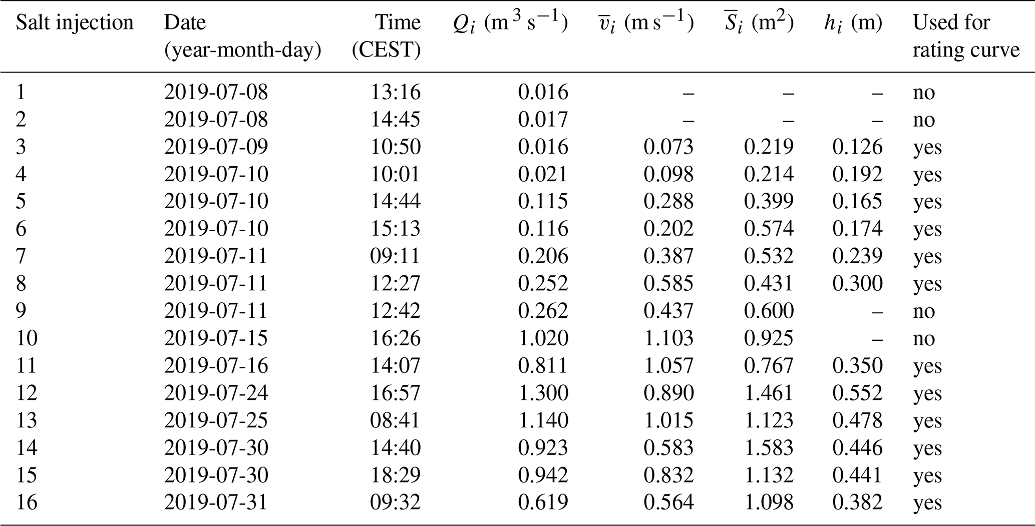
Table B1 presents the salt dilution experiments conducted to determine the discharge Q_i at station P3 and the velocity ${\stackrel{\mathrm{‾}}{v}}_i$ and the wetted cross-section ${\stackrel{\mathrm{‾}}{S}}_i$ averaged between stations P5 and P3. These quantities are in turn used to characterize the hydraulics (calculation of Reynolds number Re and the Darcy–Weisbach friction factor f_D) and the thermodynamics (calculation of the Nusselt number Nu) of the supraglacial channel. Other salt dilution experiments conducted at stations P2 and P1 were used to validate the rating curve (Eq. 4) and are presented in the “Code and data availability” section.

Table B1 Table of salt dilution experiments conducted to determine Q_i at station P3 and to obtain ${\stackrel{\mathrm{‾}}{v}}_i$ and ${\stackrel{\mathrm{‾}}{S}}_i$ averaged between stations P5 and P3. Salt dilution experiments at P3 were used for the rating curve (Eq. 4) when water stage h_i was available at the same moment and at the same location. The accuracy for Q_i and ${\stackrel{\mathrm{‾}}{S}}_i$ is typically 4 %. The accuracy for h_i is 0.005 m.