Penetration of interferometric radar signals in Antarctic snow

Synthetic aperture radar interferometry (InSAR) is an efficient technique for mapping the surface elevation and its temporal change over glaciers and ice sheets. However, due to the penetration of the SAR signal into snow and ice, the apparent elevation in uncorrected InSAR digital elevation models (DEMs) is displaced versus the actual surface. We studied relations between interferometric radar signals and physical snow properties and tested procedures for correcting the elevation bias. The work is based on satellite and in situ data over Union Glacier in the Ellsworth Mountains, West Antarctica, including interferometric data of the TanDEM-X mission, topographic data from optical satellite sensors and field measurements on snow structure, and stratigraphy undertaken in December 2016. The study area comprises ice-free surfaces, bare ice, dry snow and firn with a variety of structural features related to local differences in wind exposure and snow accumulation. Time series of laser measurements of NASA's Ice, Cloud and land Elevation Satellite (ICESat) and ICESat-2 show steady-state surface topography. For area-wide elevation reference we use the Reference Elevation Model of Antarctica (REMA). The different elevation data are vertically co-registered on a blue ice area that is not affected by radar signal penetration. Backscatter simulations with a multilayer radiative transfer model show large variations for scattering of individual snow layers, but the vertical backscatter distribution can be approximated by an exponential function representing uniform absorption and scattering properties. We obtain estimates of the elevation bias by inverting the interferometric volume correlation coefficient (coherence), applying a uniform volume model for describing the vertical loss function. Whereas the mean values of the computed elevation bias and the elevation difference between the TanDEM-X DEMs and the REMA show good agreement, a trend towards overestimation of penetration is evident for heavily wind-exposed areas with low accumulation and towards underestimation for areas with higher accumulation rates. In both cases deviations from the uniform volume structure are the main reason. In the first case the dense sequence of horizontal structures related to internal wind crust, ice layers and density stratification causes increased scattering in near-surface layers. In the second case the small grain size of the top snow layers causes a downward shift in the scattering phase centre.

1 Introduction

Digital elevation models (DEMs) derived from across-track interferometric synthetic aperture radar (InSAR) data are a main data source for mapping the surface elevation and its temporal change over glaciers and ice sheets. Single-pass InSAR systems, such as the TanDEM-X (TDM) mission, are of particular interest for this task as they are not affected by variations in the atmospheric phase delay, ice motion and temporal decorrelation. For the analysis and interpretation of InSAR elevation over snow and ice, the effects of signal penetration have to be taken into account. The surface inferred from uncorrected InSAR elevation data refers to the position of the scattering phase centre in the snow–firn medium, resulting in an elevation bias versus the actual surface (Dall, 2007). The position and strength of scattering sources in the snow volume and the absorption and scattering losses are main factors defining the depth of the phase centre below the snow surface. Backscatter contributions from sources at different depths within a volume-scattering medium, observed under different incidence angles, are causing decorrelation, depending on the interferometric baseline and incidence angle (Bamler and Hartl, 1998).

Hoen and Zebker (2000, 2001) derived a formulation for estimating the power penetration depth in dry snow from the interferometric coherence, applying a radiative transfer model for estimating spatial decorrelation in a volume of uniformly distributed and uncorrelated scatterers characterised by exponential extinction. They applied this formulation to derive the C-band penetration depth for different sites in Greenland from the coherence of 3 d repeat-pass InSAR data of the ERS-1 synthetic aperture radar (SAR) mission. Forsberg et al. (2000) and Dall et al. (2001) compared surface elevation measured by airborne laser altimetry and C-band single-pass SAR interferometry on the Geiki ice cap in Greenland. They report zero InSAR elevation bias for wet snow and an average bias of about 10 m for dry snow and firn. Dall (2007) studied relations between the InSAR elevation bias and the power penetration depth in uniform volumes. He shows that the depth of the mean phase centre in a volume-scattering medium is approximately equal to the two-way penetration depth if the latter is smaller than about 10 % of the height of ambiguity (H_a), the height difference for a phase shift of 2π. Fischer et al. (2019a, b, 2020) studied various concepts for characterising and modelling the vertical backscatter distribution and retrieving the InSAR penetration bias in the percolation zone of Greenland based on airborne polarimetric multi-baseline InSAR data and in situ measurements of snow structural properties.

In recent years single-pass InSAR data of the TDM mission were widely applied for mapping surface elevation and elevation change on glaciers and ice sheets. The TDM mission employs a bistatic interferometric configuration of the two satellites TerraSAR-X and TanDEM-X flying in close formation in order to form a single-pass SAR interferometer (Krieger et al., 2013). Rizzoli et al. (2017b) compared surface elevation over Greenland measured by NASA's Ice, Cloud and land Elevation Satellite (ICESat) laser altimeter with the TanDEM-X global DEM. They report for frozen snow and firn in the wet snow zone, the lower and upper percolation zone, and the dry-snow zone mean values of the X-band InSAR penetration bias of 3.7, 3.9, 4.7 and 5.4 m, respectively. Abdullahi et al. (2019) use a linear regression model for estimating the elevation bias in TDM DEMs of northern Greenland. The model is based on empirical relations between coherence and backscatter intensity with the difference between the uncorrected TDM DEMs and airborne laser altimeter surface heights.

The complex layered structure of polar snow and firn has a major impact on radar signal propagation and interferometric coherence, an obstacle for establishing a generally applicable, physically based method for estimating the elevation bias of InSAR products. The work presented in this paper takes on this open issue, exploring relations between interferometric parameters and physical snow properties and investigating the feasibility of deducing the elevation bias from the interferometric correlation. The study is based on interferometric data of the TDM mission, data from optical satellite sensors and field measurements undertaken in December 2016 on Union Glacier in the Ellsworth Mountains, Antarctica. Logistic support was provided by the private company Antarctic Logistics & Expeditions LLC (ALE), which conducts aircraft flights to Union Glacier and operates a field station in summer. The study area comprises ice-free surfaces, bare ice, dry snow and firn, exhibiting a diversity of structural features attributed to local differences in wind exposure and snow accumulation. Time series of ICESat laser measurements from 2003 to 2009 and ICESat-2 data show near-steady-state surface topography, facilitating the intercomparison of TDM and optical elevation data.

In Sect. 2 we describe the study area, present details on the satellite data, and give an account of the structure and morphology of snow and firn at different sites. Section 3 explains the basic concept relating the elevation bias and interferometric coherence in a uniform random volume. Section 4 deals with vertical co-registration of the different DEMs, including an analysis of the temporal stability of surface elevation, and describes the observed spatial pattern of the backscatter signals, coherence and elevation bias. Section 5 presents results of the inversion of the volumetric coherence in terms of the InSAR elevation bias and compares the retrieved bias with elevation differences between TDM DEMs and optical data. Section 6 includes the discussion, and Sect. 7 presents conclusions. The Appendix shows simulations for vertical backscatter distributions at snow pit sites and compares these with exponential backscatter functions.

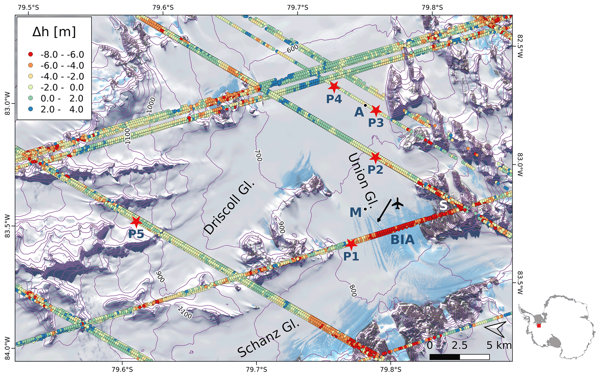
Figure 1 Landsat 8 image acquired on 6 December 2016 (composite of bands 5, 4, 2) with ICESat tracks. Points: elevation difference Δh (ICESat minus TDM global DEM), colour-coded from $\mathrm{\Delta }h=-\mathrm{8}$ to +4 m. P1 to P5: locations of snow pits. A: ALE camp; BIA: blue ice area; M: recording meteorological station; S: ice-free slope. The arrow points to the landing strip.

2 Study area and data

2.1 Surface mass balance and orographic effects

Union Glacier flows from the ice divide in the Heritage Range, Ellsworth Mountains, down to the Constellation Inlet on Ronne Ice Shelf. The glacier section immediately downstream of the main mountain range is exposed to strong katabatic winds so that bare ice appears on the surface (Fig. 1). The blue ice area (BIA) has a negative specific surface mass balance, b_n, on the order of several centimetres water equivalent (w.e.) per year due to sublimation (Rivera et al., 2014). In the BIA an ice runway for landing heavy airplanes on wheels is maintained from November to March. The ALE camp is located 8 km downstream of the ice runway.

GPS measurements at stakes, performed during the period 2007 to 2011, show ice velocities on the order of 20 m a⁻¹ at the glacier gate across the runway (Rivera et al., 2010, 2014). For 2008 to 2012 a mean wind speed of 16.3 knots with predominant direction from the south-west (blowing downstream along the main glacier) was measured at an automatic station close to the runway. Wind speed and direction are very consistent. Rivera et al. (2014) report a mean b_n of −0.10 m w.e. a⁻¹ measured at 29 stakes in the BIA during 2007 to 2011. The intensity of the katabatic winds declines downstream of the BIA so that snow accumulates, and the surface mass balance is positive. Accumulation measurements in 2008–2009 at four stakes located on the main glacier 4.5, 7.0, 10.5 and 15 km downstream of the BIA show b_n values 0.20, 0.13, 0.17 and 0.14 m w.e. a⁻¹ (Rivera et al., 2014). Hoffmann et al. (2020) collected and analysed six shallow ice cores in the wider Union Glacier region. One of the cores was drilled on Union Glacier itself about 2 km west of P3, showing for 1989 to 2013 mean b_n of 0.18 m w.e. a⁻¹.

Differences in the exposure to wind are a main factor for local variations in the accumulation rate and in the structural properties of snow and firn. This is evident in differences in the microstructure and stratigraphy observed in snow pits, ranging from coarse-grained dense snow with wind crusts near the runway (pit P1), located in the main pathway of the katabatic wind, to finer-grained and softer snow at P5 on a lateral slope of Driscoll Glacier. Accumulation estimates at P5 for 2015 and 2016, deduced from snow pit data, show a mean b_n of about 0.4 m w.e. a⁻¹ (Sect. 2.4).

Uribe et al. (2014) operated two radar sensors during an over-snow campaign in December 2010, measuring the total ice thickness and the thickness and structure of the firn layers along an 82 km track, starting on Union Glacier and proceeding along Driscoll and Schanz glaciers up to the Ellsworth Plateau. The total thickness of the firn layer varies significantly along this track, even within short distances. For example, a radargram along a 6 km transect extending from the confluence with Driscoll Glacier across Union Glacier towards the camp shows thickness values of the snow–firn layer ranging from zero on blue ice at the confluence of the two glaciers to a maximum of 34 m close to the camp, increasing gradually with distance.

2.2 TanDEM-X data

The TDM data for this study comprise one tile of the TDM global (TDMgl) DEM, the primary product of the TDM mission, and raw SAR data from several dates for compiling topography, backscatter intensity and coherence products. We use the TDMgl DEM for topographic corrections and geocoding because it provides full spatial coverage, whereas the DEMs of individual dates have gaps, depending on the observation geometry. The data from individual dates are used for studying the impact of specific interferometric configurations on the coherence, backscatter signatures and penetration bias. Tile TDM1_DEM_04_S80W084_V01_C of the global DEM is used, extending from 79 to 80^∘ S and 82 to 84^∘ W and referring to the coordinate reference system WGS 84 (G1150). This tile was obtained by mosaicking multiple single DEM scenes acquired between 6 May 2013 and 23 August 2014. The pixel spacing is 0.4 arcsec in northing and 1.2 arcsec in easting, corresponding to 12.4 m×6.5 m at 80^∘ latitude. For the TDMgl elevation products over ice sheets, penetration corrections were applied, using ICESat data as an elevation reference (Wessel et al., 2016; Rizzoli et al., 2017a). For Antarctica (excluding coastal regions) a mean penetration bias was derived for each of the 11 extended homogeneous areas (fixed blocks) located in different sections of the ice sheet. For the areas in between, the elevation is adjusted by spatial interpolation between these blocks, regionally applying bulk values that are not accounting for different surface types (Rizzoli et al., 2017a).

For producing DEMs from raw bistatic SAR data (Level 0) of individual tracks (the so-called Raw DEMs), we used the operational Integrated TanDEM-X Processor (ITP) of the German Aerospace Center (DLR) (Rossi et al., 2012). The Raw DEM pixel spacing is 6 m×3 m. Complementary to each Raw DEM, the ITP provides geocoded rasters of the height error (the height error map, HEM), the SAR amplitude, the backscattering coefficient and the interferometric coherence as well as a flag mask indicating critical areas. We applied 11×11 pixel estimation windows for computing the coherence maps, adding up to about 390 independent samples for single-polarised data at a 40^∘ incidence angle and about 110 independent samples for dual-polarised data at a 22^∘ incidence angle. According to the Cramér–Rao bound for coherence estimation, the standard deviation for a coherence magnitude of 0.5 amounts to 0.03 for the first case and 0.05 for the second case. The uncertainty decreases towards higher coherence values (Bamler and Hartl, 1998). The backscatter intensity images show maps of the normalised radar cross-section σ^∘. For the computation of σ^∘, effects of topography are taken into account for antenna pattern removal and for defining the actual size of the local scattering area. The absolute and relative radiometric accuracies for the TerraSAR-X strip map data are estimated at 0.6 and 0.3 dB, respectively (Breit et al., 2010).

The HEM delivers the height errors for each DEM pixel caused by random noise. It is given by the standard deviation of the interferometric phase, for which the coherence and the number of looks are the main factors. The HEM accounts neither for the absolute height error (offset) with respect to a particular geodetic reference system nor for penetration-related errors. Low-pass filtering is an efficient means for reducing the random height error. The HEM for the TDMgl DEM of the study region shows over flat terrain and gentle slopes random height errors ranging from 0.3 to 1.2 m.

Table 1 Specifications of TanDEM-X data used for DEM production and generation of backscatter and coherence images. θ_i is the incidence angle in the scene centre. B_n is the effective interferometric baseline, H_a is the height of ambiguity, and k_zVol is the vertical interferometric wavenumber in the snow volume assuming a density of 400 kg m⁻³. SAR operation mode: bistatic; HH: horizontal transmit and receive polarisation; VV: vertical transmit and receive polarisation.

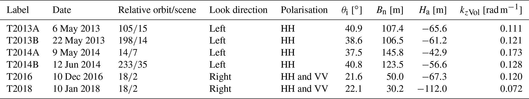
Specifications of the TDM data used in this study are listed in Table 1. The azimuth resolution of the single-polarisation data is 3.3 m and of the dual-polarised data 6.6 m. The ground range resolution is 3.20 m at θ_i=22^∘ and 1.86 m at θ_i=40^∘. We selected scenes with different incidence angles and baselines in order to check the impact of these parameters on coherence, backscatter intensity and signal penetration. According to the HEM maps, the random errors for the Raw DEMs, excluding steep slopes, range from 0.7 to 3.0 m. The spatial variations can mainly be attributed to phase noise arising from thermal and volume decorrelation. For the estimation of signal penetration we use averages over multiple pixel windows in order to reduce the uncertainty.

2.3 Topographic data from optical satellite sensors

Topographic data from the ICESat and ICESat-2 missions and the Reference Elevation Model of Antarctica (REMA), derived from very-high-resolution optical stereo images (Howat et al., 2019), are available as a reference for estimating the elevation bias in the InSAR DEMs. We use the ICESat and ICESat-2 data primarily for assessing the temporal stability of surface elevation. The study area is covered by several tracks of the ICESat and ICESat-2 altimeters. Elevation data were acquired by ICESat during several campaigns between April 2003 and October 2009. We use GLAH12 GLAS/ICESat L2 Global Antarctic and Greenland Ice Sheet Altimetry Data (HDF5), Release 34 (Zwally et al., 2014). This product provides geolocated and time-tagged surface elevation estimates, referenced to the TOPEX/Poseidon ellipsoid and corrected for atmospheric delays and tides. The laser footprint size is 60 to 70 m, and the distance between the footprint centres is approximately 170 m. The analysis of repeat-track data allows the detection of the surface elevation change after correcting for elevation differences caused by horizontal shifts in individual footprints. A main cause for the height error in ICESat footprints is the uncertainty in beam pointing, causing slope-induced errors (Brenner et al., 2007; Zwally et al., 2011).

Regarding ICESat-2, we use ATLAS/ICESat-2 L3A Land Ice Height, Version 2, Land Ice Along-Track Height (ATL06) product from the time span 14 October 2018 to 1 September 2019. This data set provides geolocated land-ice surface heights above the WGS 84 ellipsoid, ITRF2014 reference frame, and ancillary parameters including error estimates and quality flags (Smith et al., 2019a). ATL06 heights represent the mean surface height averaged along 40 m segments of ground track, 20 m apart, for each of the six beams of the Advanced Topographic Laser Altimeter System (ATLAS) instrument. The land-ice height is defined as estimated surface height of the segment centre for each reference point (Smith et al., 2019b).

For spatially detailed comparisons of elevation we use the REMA DEM tile no. 32-19 with 8 m posting, covering Union Glacier (Howat et al., 2019). The dates of the image acquisitions for this tile range from January 2014 to December 2015. The absolute height is based on vertical registration to CryoSat-2 altimetry data, acquired in SAR interferometric (SARIn) mode. In order to account for the CryoSat signal penetration, a uniform value of 0.39 m was added to the CryoSat-2-registered heights over this tile, regardless of the surface type (Howat et al., 2019). This needs to be taken into account for using the REMA data as an elevation reference because the study area includes bare ground, ice surfaces, and snow and firn with different structural properties affecting radar signal penetration. The vertical error estimates for REMA in the region of interest range from 1.0 to 1.4 m. The error value of each pixel is the standard error from the residuals of the registration to altimetry (Howat et al., 2019). The error due to the use of the bulk CryoSat-2-based penetration correction is not included in this error estimate.

2.4 Snow pit measurements

For the snow pit measurements, made in December 2016, we selected sites covered by ICESat footprints that show different values of coherence and backscatter intensity in TDM data. Backscatter properties of dry snow and firn are controlled by snow microstructure, which is also a main factor for X-band radar signal penetration. In the study region the impact of melt for snow metamorphism is marginal. We detected evidence for melt events in two of the five snow pits: a thin ice crust at 1.1 m depth of pit 5 and two thin ice crusts along with one ice layer of 4 cm thickness in pit 1. The temperature record from March 2010 to February 2014 at the meteorological station near the runway shows a mean annual air temperature of −21.1 ^∘C and mean monthly temperatures of −8.6 ^∘C for December and −9.3 ^∘C for January. During those years a few short events with air temperatures close to the melting point were recorded.

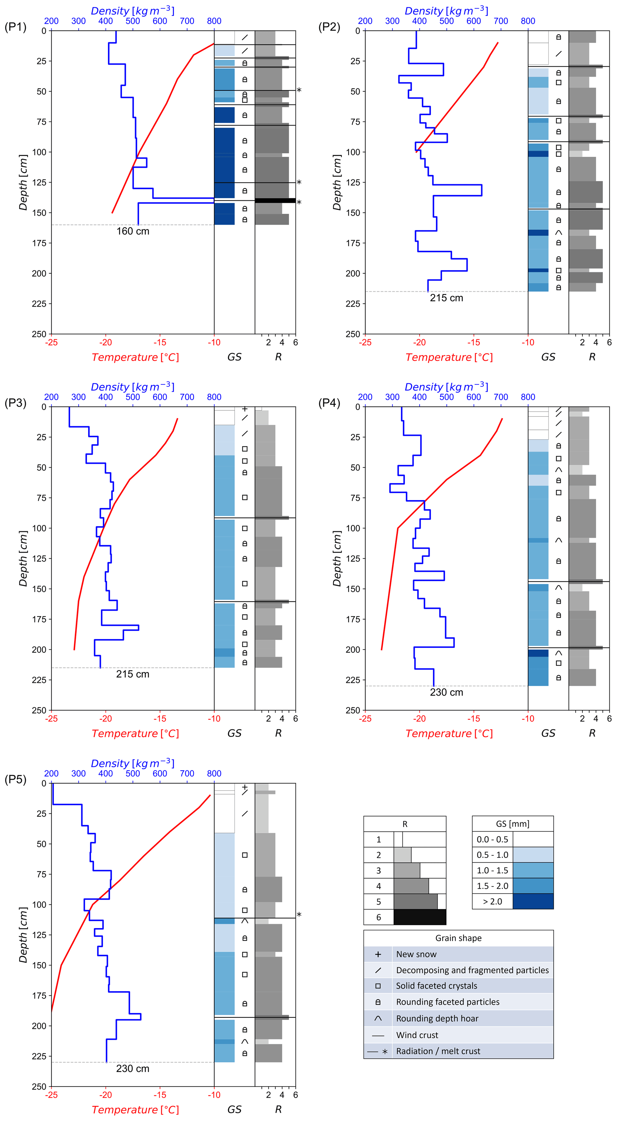
Figure 2 Vertical profiles of snow temperature, density, grain size (GS), grain shape and hand hardness (R) for snow pits P1 to P5 on Union Glacier, December 2016. The grain size refers to the maximum axis length of the prevailing snow grains.

Table 2 Mean density of snow–firn for layers of 0.5 m vertical extent of snow pits P1 to P5 on Union Glacier. The snow pit altitude refers to the REMA DEM.

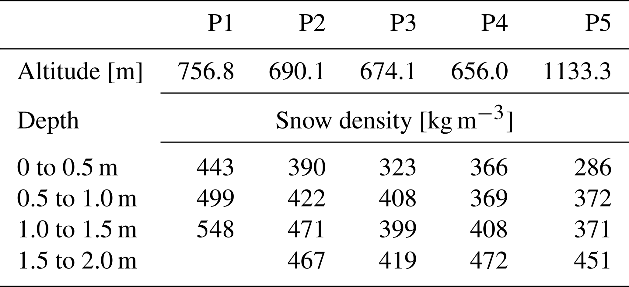
Profiles of snow density, temperature, hardness, grain size and shape are shown in Fig. 2. The pits vary in depth between 1.6 and 2.3 m. The observed grain size refers to the maximum axis length of prevailing grains (Fierz et al., 2009). Hardness was estimated by the hand test, ranging from very low (R1) to very high (R5) for snow and R6 for ice. The mean density of snow–firn for layers of 0.5 m vertical extent is specified in Table 2. Grain size and hardness show significant differences between the five measurement sites. The size and shape of the snow grains and the sequence and properties of snow–firn layers are arising from accumulation history, exchange processes of radiation, turbulent heat and mass at the snow–air interface, and vapour diffusion in the snow volume. Down to about 2 m depth the temperature gradient metamorphism is the dominating process for grain growth, triggered by seasonal temperature variations (Alley, 1988; Colbeck, 1983). Average temperature gradients in the top metre of the five snow pits were on the order of 10 ^∘C m⁻¹. Differences in the average grain size of the pits can, at least partly, be attributed to the snow age following from differences in the surface mass balance (Sect. 2.1). Courville et al. (2007) studied the microstructure of snow and firn in a megadune region in East Antarctica. They show that local differences in grain size, thermal conductivity and permeability are related to spatial accumulation variability in which already relatively small differences in the net accumulation due to wind redistribution cause significant differences in physical snow properties.

Snow pit 1 exhibits the largest grains, the highest snow density, thin ice layers and several wind crusts. Accumulation data are not available, but from the closeness to the BIA it can be concluded that the mean accumulation rate is well below the accumulation rate near the ALE camp. Due to the high exposure to katabatic winds the stratification does not allow an identification of annual accumulation layers. In some years sublimation and wind erosion may result in negative mass balance. The higher hardness values compared to the other sites can be attributed to more frequent exposure to high wind speeds, the erosion and deposition of blowing snow, and greater age due to low accumulation. Two thin ice crusts (5 mm thickness) at 0.49 and 1.25 m depth possibly trace back to radiation penetration causing melt below the frozen surface (Colbeck, 1989). An ice layer of 4 cm thickness between 1.38 and 1.42 m depth, with air bubbles of up to 2 mm size, indicates an intensive melt event.

P2 is the snow pit with the highest average snow density next to P1. It is located halfway between the runway and the ALE camp, more exposed to katabatic winds than the camp so that the average accumulation rate should be lower than at P3 and P4. The stratigraphy down to 2 m depth shows four layers of high density with comparatively fine-grained snow, typical for wind packs, and several thin wind crusts. Softer layers with faceted grains show up below wind packs, but a clear assignment to seasonal or annual layers is not possible.

The pits P3 and P4, located in the vicinity of the camp, show lower mean density and lower variability in density. P4 is located slightly upstream of stake B10, for which Rivera et al. (2014) report a specific mass balance b_n=0.17 m w.e. a⁻¹ for 2008–2009. Down to the depth of 2.0 m the P4 stratification shows four comparatively thick, hard layers with rounding depth hoar below. The total snow mass down to 2.0 m amounts to 0.81 m w.e. Assuming that the transitions from hard to soft layers correspond to late summer horizons and accounting for the lack of 2 months to cover the full 4-year period imply an annual accumulation rate b_n=0.21 m w.e. a⁻¹. At P3 the sequence of layers is less distinct. This site is located at a cross-wind distance of 300 m from the camp and may be affected by local perturbations of snow drift during summer, when the camp is set up to a full extent.

P5 is located at 1133 m elevation on a flat section of a slanting lateral branch of Driscoll Glacier that extends uphill towards the Pioneer Heights, 400 m in altitude above the confluence with Union Glacier. The site is not exposed to the strong katabatic winds that are blowing along the main branch of Union Glacier. The grain size is smaller, and the snow is softer than at the other sites. A melt crust of 3 mm thickness was found at 1.14 m depth, most likely related to a short event with comparatively warm temperatures on 17–18 January 2016. The snow mass above this crust amounts to 0.38 m w.e. A thin hard layer at 2.11 m depth with a soft, coarse-grained layer below refers probably to the 2015 late-summer horizon. The snow mass between the wind crust in late summer 2015 and the melt crust in January 2016, a period of about 11 months, amounts to 0.41 m w.e. These two accumulation estimates indicate for this site about twice the accumulation rate on the main glacier near the ALE camp.

3 Interferometric coherence and penetration-related elevation bias

The procedure for estimating the interferometric elevation bias is based on the inversion of the volumetric correlation factor, which can be derived from total coherence products (γ_tot) generated during InSAR processing. The total interferometric complex correlation coefficient (coherence) of a random medium is made up of the following contributions (Krieger et al., 2007):

$$\begin{array}{}\text{(1)}& {\mathit{\gamma }}_{\mathrm{tot}}={\mathit{\gamma }}_{\mathrm{therm}}\cdot {\mathit{\gamma }}_{\mathrm{Quant}}\cdot {\mathit{\gamma }}_{\mathrm{Amb}}\cdot {\mathit{\gamma }}_{\mathrm{Rg}}\cdot {\mathit{\gamma }}_{\mathrm{Az}}\cdot {\mathit{\gamma }}_{\mathrm{Vol}}\cdot {\mathit{\gamma }}_{\mathrm{temp}}.\end{array}$$

The terms on the right-hand side refer to the interferometric correlation coefficient related to the signal-to-noise ratio (γ_therm), quantisation (γ_Quant), azimuth and range ambiguities (γ_Amb), baseline decorrelation (γ_Rg), relative shift in the Doppler spectra (γ_Az), volumetric decorrelation (γ_Vol), and temporal decorrelation (γ_temp). Temporal decorrelation is not relevant for single-pass InSAR data over ground, including snow and ice (γ_temp=1.0).

The thermal interferometric correlation component is related to the signal-to-noise ratio (SNR) of the two SAR images by

$$\begin{array}{}\text{(2)}& {\mathit{\gamma }}_{\mathrm{therm}}=\mathrm{1}/\sqrt{\left(\mathrm{1}+{\text{SNR}}_{\mathrm{1}}^{-\mathrm{1}}\right)\left(\mathrm{1}+{\text{SNR}}_{\mathrm{2}}^{-\mathrm{1}}\right)}.\end{array}$$

For single-pass InSAR the volumetric correlation coefficient can be derived from the total coherence by

$$\begin{array}{}\text{(3)}& {\mathit{\gamma }}_{\mathrm{Vol}}={\displaystyle \frac{{\mathit{\gamma }}_{\mathrm{tot}}}{{\mathit{\gamma }}_{\mathrm{therm}}{\mathit{\gamma }}_{\mathrm{Quant}}{\mathit{\gamma }}_{\mathrm{Amb}}{\mathit{\gamma }}_{\mathrm{Rg}}{\mathit{\gamma }}_{\mathrm{Az}}}}.\end{array}$$

The phase noise due to γ_Amb, γ_Quant and γ_Az of advanced SAR systems is small. For TDM single-pass InSAR interferograms Krieger et al. (2007) estimate the typical loss of coherence for each of the terms γ_Amb, γ_Quant and γ_Az at <2 %. Baseline decorrelation, γ_Rg, is avoided by applying common bandwidth filtering.

Hoen and Zebker (2000) specify a formulation for the correlation factor in a uniform volume with exponential extinction in which the interferometric phase is proportional to the penetration length, d_l:

$$\begin{array}{}\text{(4)}& \begin{array}{rl}{\mathit{\gamma }}_{\mathrm{Vol}}& =\mathrm{1}/\sqrt{\mathrm{1}+{\left({\displaystyle \frac{p\mathit{\pi }\sqrt{\mathit{\epsilon }}{d}_{\mathrm{l}}{B}_{\mathrm{n}}}{r_{\mathrm{0}}\mathit{\lambda }\tan {\mathit{\theta }}_{\mathrm{i}}}}\right)}^{\mathrm{2}}}\\ & =\mathrm{1}/\sqrt{\mathrm{1}+{\left({\displaystyle \frac{\mathit{\pi }\sqrt{\mathit{\epsilon }}{d}_{\mathrm{l}}\cos {\mathit{\theta }}_{\mathrm{i}}}{H_{\mathrm{a}}}}\right)}^{\mathrm{2}}},\end{array}\end{array}$$

where λ is the radar wavelength, r₀ is the slant range distance, θ_i is the incidence angle at the air–snow interface, B_n is the effective interferometric baseline, and ε is the dielectric permittivity; p=1 is valid for the combination of one monostatic and one bistatic SAR image forming an interferogram and p=2 for the combination of two monostatic images. H_a is the height of ambiguity in free space:

$$\begin{array}{}\text{(5)}& H_{\mathrm{a}}={\displaystyle \frac{\mathit{\lambda }{r}_{\mathrm{0}}\sin {\mathit{\theta }}_{\mathrm{i}}}{p{B}_{\mathrm{n}}}}.\end{array}$$

According to the radiative transfer approach the one-way power penetration length d_l [m], where the intensity of the signal is attenuated to $\mathrm{1}/e$ of the incident signal, is given by

$$\begin{array}{}\text{(6)}& d_{\mathrm{l}}={\displaystyle \frac{\mathrm{1}}{k_{\mathrm{e}}}}={\displaystyle \frac{\mathrm{1}}{k_{\mathrm{s}}+k_{\mathrm{a}}}},\end{array}$$

where k_a and k_s [m⁻¹] are the absorption and the scattering coefficients. The one-way power penetration depth, d_p, referring to vertical direction, is obtained by accounting for the refraction angle θ_r:

$$\begin{array}{}\text{(7)}& d_{\mathrm{p}}=d_{\mathrm{l}}\cos {\mathit{\theta }}_{\mathrm{r}}.\end{array}$$

The vertical interferometric wavenumber, k_z [rad m⁻¹], relates the phase of the interferometric correlation to the geometric configuration of the interferometer, providing phase (φ) to height conversion:

$$\begin{array}{}\text{(8)}& k_z={\displaystyle \frac{\partial \mathit{\phi }}{\partial z}}={\displaystyle \frac{\mathrm{2}\mathit{\pi }}{H_{\mathrm{a}}}}.\end{array}$$

The wavenumber in a lossy volume accounts for the change in the propagation constant and refraction (Lei at al., 2016), yielding the following formulation for the height of ambiguity in the volume:

$$\begin{array}{}\text{(9)}& H_{\mathrm{aVol}}={\displaystyle \frac{\mathrm{2}\mathit{\pi }}{k_{z\mathrm{Vol}}}},\end{array}$$

where

$$k_{z\mathrm{Vol}}=k_z\sqrt{\mathit{\epsilon }}{\displaystyle \frac{\cos {\mathit{\theta }}_{\mathrm{i}}}{\cos {\mathit{\theta }}_{\mathrm{r}}}}.$$

For dry snow and ice the absorption, losses are very small so that the real part of the permittivity can be used (Mätzler, 1996). In Table 1 the values for H_a and for k_zVol (assuming a snow density of 400 kg m⁻³) are specified for the TDM scenes.

Dall (2007) shows that the penetration-related elevation bias, h_b, is approximately equal to the two-way power penetration depth, d_p2, if the latter is small compared to H_aVol. For large relative penetration depths ($d_{\mathrm{p}\mathrm{2}}/H_{\mathrm{aVol}}$) the elevation bias approaches one-quarter of the ambiguity height. Normalising the coherence phase, ∠γ, by the interferometric phase at the volume surface ($\mathrm{\angle }\mathit{\gamma }=\mathit{\phi }-{\mathit{\phi }}_{\mathrm{surface}}$) yields the following relation, in which the elevation bias is proportional to ∠γ (Dall, 2007):

$$\begin{array}{}\text{(10)}& h_{\mathrm{b}}=\mathrm{\angle }\mathit{\gamma }/k_{z\mathrm{Vol}}={\displaystyle \frac{\mathrm{\angle }\mathit{\gamma }\left|H_{\mathrm{aVol}}\right|}{\mathrm{2}\mathit{\pi }}}.\end{array}$$

For a uniform volume a direct relationship between the coherence magnitude and the relative penetration depth can be defined, from which the phase can be computed (Dall, 2007):

$$\begin{array}{}\text{(11)}& \mathrm{\angle }\mathit{\gamma }=-\text{sgn}\left(H_{\mathrm{aVol}}\right)\text{arctan}\left(\sqrt{{\left|{\mathit{\gamma }}_{\mathrm{Vol}}\right|}^{-\mathrm{2}}-\mathrm{1}}\right).\end{array}$$

As according to this relation the coherence phase is uniquely defined by the coherence magnitude, the following formulation can be used for estimating the elevation bias:

$$\begin{array}{}\text{(12)}& h_{\mathrm{b}}=-\left|{\displaystyle \frac{H_{\mathrm{aVol}}}{\mathrm{2}\mathit{\pi }}}\right|\text{arctan}\left(\sqrt{{\left|{\mathit{\gamma }}_{\mathrm{Vol}}\right|}^{-\mathrm{2}}-\mathrm{1}}\right).\end{array}$$

We apply this equation for estimating the elevation bias from the observed coherence, using the magnitude of the volumetric InSAR correlation factor as input. According to this formulation the actual InSAR elevation bias becomes progressively smaller than d_p2 with increasing relative penetration depth.

This approach is based on the assumption of a uniform volume with exponential extinction, whereas dry polar firn is a density-stratified medium featuring distinct differences in scattering and extinction properties between individual layers as well as depth-dependent changes. However, for inverting the observed interferometric coherence in terms of the elevation bias the assumption of a simple model is needed for describing the vertical backscatter and extinction properties. We tested the applicability of the uniform volume approach for describing the observed backscatter intensity, performing forward computations with a multilayer radiative transfer model (see Appendix A).

4 Analysis of backscatter signatures, coherence and elevation bias

In this section we show the spatial pattern of backscatter intensity and coherence in the study area and relations of these parameters to the elevation bias inferred from optical sensor data. We start with an account of topographic reference data and the procedures applied for vertical co-registration, a critical step for estimating the penetration-related elevation bias.

4.1 Topographic reference and vertical co-registration

The precise vertical co-registration on surfaces that are not subject to radar signal penetration is essential for obtaining reliable estimates on the interferometric elevation bias. If the data to be co-registered are lacking temporal coincidence, checks on the temporal stability of the surfaces are needed. These topics are addressed below.

4.1.1 Notations for elevation differences

The apparent glacier surface in an InSAR DEM refers to the position of the scattering phase centre in the snow and firn volume. The elevation bias, h_b, is the difference between the apparent elevation derived by means of the InSAR method, h_insar, and the true surface elevation, h_s:

$$\begin{array}{}\text{(13)}& h_{\mathrm{b}}=h_{\mathrm{insar}}-h_{\mathrm{s}}.\end{array}$$

For the elevation bias estimate derived from the volumetric coherence by means of Eq. (12) we use the notation h_bInv. For studying the penetration-related elevation bias we co-register the TDM DEMs on surfaces devoid of penetration with elevation data of optical sensors. On these surfaces the raw TDM DEMs show vertical offsets up to a few metres because for these data only a preliminary adjustment for absolute height is performed with ITP processing. We use the notation Δh for specifying the elevation difference between optical data and the vertically unregistered TDM DEMs:

$$\begin{array}{}\text{(14)}& \mathrm{\Delta }h=h_{\mathrm{optical}}-h_{\mathrm{TDM},\mathrm{unreg}}.\end{array}$$

Suitable targets for vertical co-registration in the study area are the BIA and bare ground on an ice-free slope bordering the BIA (“S” in Fig. 1). We use the notation dh for the elevation difference between the TDM DEMs and optical elevation data, vertically co-registered on surface scattering targets:

$$\begin{array}{}\text{(15)}& \mathrm{d}h=h_{\mathrm{TDM},\mathrm{coreg}}-h_{\mathrm{optical}}.\end{array}$$

In the case of temporal coincidence or stable topography, dh corresponds to the interferometric elevation bias. Though the time series of ICESat data indicate temporal stability of surface elevation in the study area, minor errors due to temporal changes in elevation cannot be fully excluded.

4.1.2 Temporal stability of surface elevation

Because of the lack of temporal coincidence between the TDM and optical elevation data, we checked the temporal variability using ICESat time series. The main section of the BIA was crossed by ICESat repeat tracks on seven dates between May 2004 and November 2009 (Fig. 1). The mean difference in elevation Δh between the ICESat footprints in the BIA and the corresponding TDMgl cells (mean values of 5×5 pixels) is −6.76 m. The standard deviation for the 126 samples of the time series is 0.43 m (Table S1 in the Supplement). The mean Δh values on the different dates range from −6.61 to −6.86 m without any distinct temporal trend, indicating high temporal stability. The stability of surface elevation in the BIA is also confirmed by the GPS time series of Rivera et al. (2014). The Δh value of −6.76 m can be mainly attributed to the bulk penetration correction that is applied for TDMgl DEM products over Antarctica. The ICESat-2 data set of the BIA includes eight tracks with altogether 345 spots, extending along the eastern and western margins of the BIA, which are occasionally covered by snow. The mean elevation difference and standard deviation are Δh (ICESat-2-TDMgl) = −6.99 m, σ_Δh=0.38 m.

In order to check the validity of the assumption that the BIA signal arises from surface scattering, we derived optical versus SAR elevation differences also on the ice-free slope in the vicinity of the BIA. This slope has a mean inclination of about 16^∘ and contains sections of varying steepness. On slopes, horizontal shifts between pixels to be co-registered cause slope-dependent elevation biases, in particular for data from sensors with different observation geometries and spatial resolution (Nuth and Kääb, 2011). Therefore we use data from moderately inclined slope sections for quantifying the vertical offsets. In order to avoid steep slope sections we excluded all cells of 5×5 TDM pixels with a standard deviation of elevation larger than 5 m. Under this constraint only 21 ICESat pixels of the whole time series qualify for the comparison on the slope, yielding a mean Δh of −6.91 m and σ_Δh of 0.84 m. The difference in the mean Δh values between the slope and the BIA is below the measurement uncertainty.

Another ICESat time series for checking the temporal behaviour of surface elevation extends across the main glacier near pit 4, where the penetration bias is several metres. The ICESat data set comprises seven closely spaced tracks acquired between 11 April 2003 and 12 February 2008. The mean value and standard deviation of the elevation difference between ICESat and the TDMgl DEM are on the central section of the glacier: Δh=0.09 m, σ_h=0.40 m (Table S2). The mean Δh values on individual dates range from −0.03 to 0.21 m without any obvious temporal trend, confirming also the temporal stability of surface elevation. Subtracting the TDMgl offset of −6.76 m from the mean Δh value (0.09 m) yields an elevation bias (dh) of −6.67 m due to signal penetration.

4.1.3 Vertical co-registration of the DEMs

We use REMA elevation data as a reference in order to obtain spatially detailed estimates of the interferometric elevation bias. The mean value and standard deviation of the elevation difference between ICESat and REMA over the BIA are $\mathrm{\Delta }h=-\mathrm{0.33}$ m, σ_Δh=0.38 m (Table S1). This value differs by 6 cm from the bulk penetration correction (−0.39 m) applied to the CryoSat-2 elevation data that are used as an absolute height reference for the REMA DEM (Howat et al., 2019). This correction introduces a bias over bare ice where the actual CryoSat-2 signal refers to surface reflection. On the ice-free slope the elevation differences in REMA versus ICESat, ICESat-2 and TDMgl elevation data show high standard deviations. Therefore we use the BIA as a reference site for vertical co-registration between the TDM DEMs and REMA.

For cross-comparing the TDM and REMA elevation data we outlined an area of 5 km² extent in the central section of the BIA that is crossed by the ICESat tracks, avoiding BIA sections that are occasionally covered by snow. The mean elevation difference Δh between REMA and TDMgl is −6.37 m; the standard deviation at 8 m×8 m pixel size is 0.62 m. We use the value of −6.37 m for vertical co-registration of the TDMgl DEM. The same polygon is used for vertical co-registration of the other TDM DEMs, which as unregistered DEMs show vertical shifts vs. REMA of −2 to −3 m.

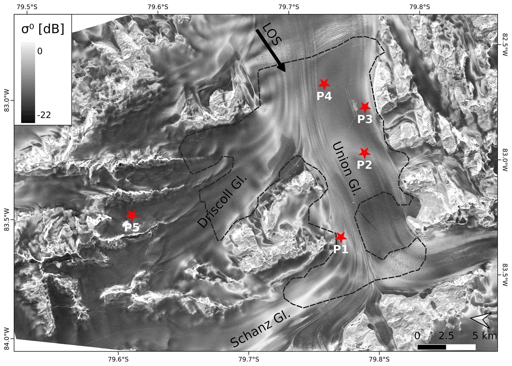
Figure 3 Section of TDM backscatter image, HH polarisation, 6 May 2013. LOS (line of sight) indicates the radar look direction. Incidence angle in the scene centre (θ_i): 40.9^∘. The outline encloses the snow and firn area of interest (AoI) for analysis of radar signatures and the elevation bias.

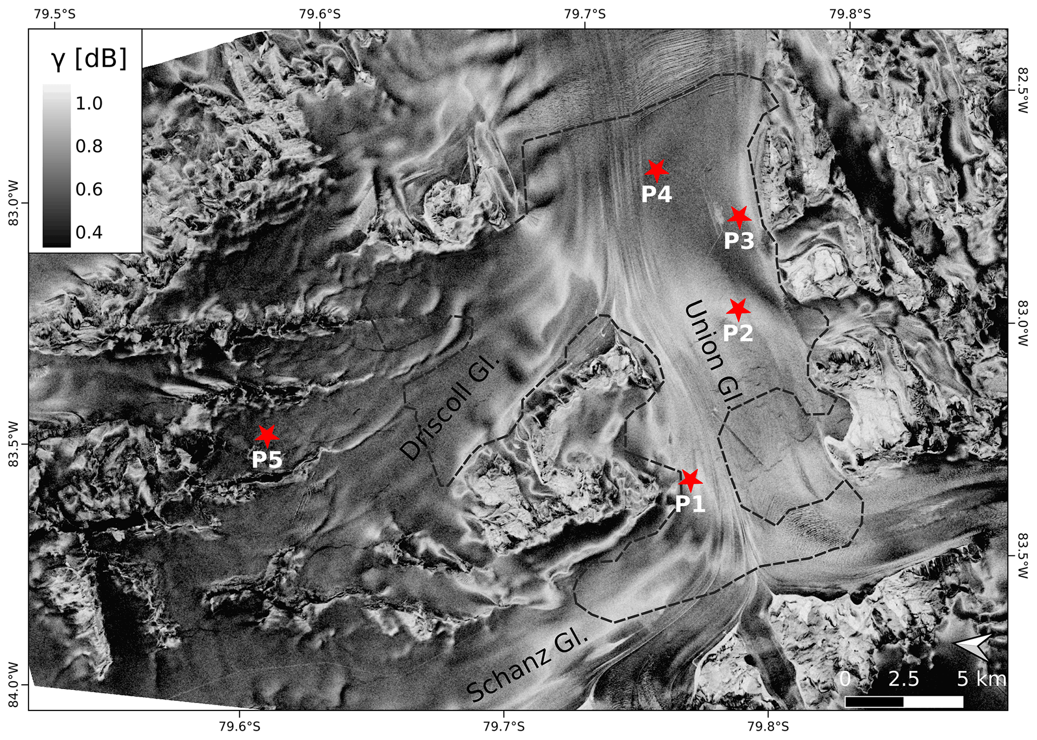
Figure 4 Image of total normalised coherence, γ_tot, from the TDM interferogram of 6 May 2013.

4.2 Spatial pattern of backscatter signals and coherence

Figure 3 shows an image of the backscatter cross-section (σ^∘) and Fig. 4 an image of the magnitude of the complex interferometric correlation coefficient (the total normalised coherence), derived from TDM data of 6 May 2013 (scene T2013A). For detailed analysis of radar signatures and the elevation bias of snow and firn, we focus on an area stretching out over sections of the main glacier and Driscoll Glacier that are completely covered by any of the available TDM scenes (the area of interest, AoI). Slopes larger than 5^∘ inclination and blue ice areas are excluded. Major blue ice areas are located in the vicinity of the landing strip, on Schanz Glacier, and at the confluence of Driscoll and Union glaciers. The slope constraint reduces impacts of errors in optical and SAR DEM co-registration and effects of foreslopes and layover that vary with the observation geometry of the different SAR tracks.

The spatial pattern of backscatter intensity in the firn areas of the main glacier and its tributaries primarily reflects differences in volume-scattering properties and to some extent also the pattern of the elevation bias (Sect. 5). Low σ^∘ values in the AoI refer to areas of comparatively fine-grained snow and firn in the top layers, whereas high values are an indication of large scattering elements. The blue ice areas have a comparatively smooth surface, accounting for low σ^∘ at an incidence angle of 40^∘. The lowest σ^∘ values show up on tributary glaciers away from the main passage of the katabatic wind. Low σ^∘ is also evident at locations of increased accumulation rates in the vicinity of the camp. At lower incidence angles σ^∘ is higher throughout, and the overall dynamic range of σ^∘ is reduced, as is evident in Fig. S1, which shows backscatter and coherence images of 10 December 2016.

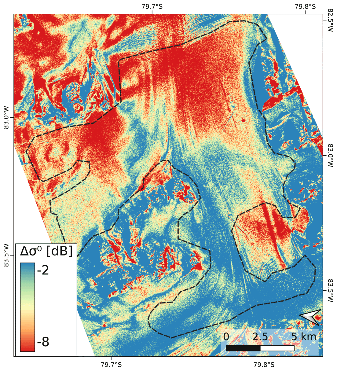
Figure 5 Difference in the HH-polarised backscatter coefficients between the TDM images from 6 May 2013 (θ_i=40.9^∘) and 10 December 2016 (θ_i=21.6^∘), σ^∘_HH 2013 minus σ^∘_HH 2016 (dB).

The incidence angle dependence of σ^∘ in the vicinity of the BIA and in crevasse zones is rather small (Fig. 5). In these areas the differences in σ^∘ between the scenes T2013A (θ_i=40.9^∘) and T2016H (θ_i=21.6^∘) amount to about 3 dB, and σ^∘ is high in both scenes. This is an indication of large scattering elements relative to the wavelength. Multiple scattering between individual layers and scattering at rough internal interfaces may also play a role. In the areas with higher accumulation rates the incidence angle dependence is larger, reaching values up to 8 dB in the vicinity of pit 4. Large angular backscatter differences in the stratified snow–firn medium can be explained by increased backscatter contributions of internal interfaces towards near-nadir angles. The pronounced σ^∘ increase towards low incidence angles in the BIA (−13.3 dB in scene T2013A, −5.9 dB in T2016H) is characteristic for backscattering of slightly rough surfaces (Fung, 1994).

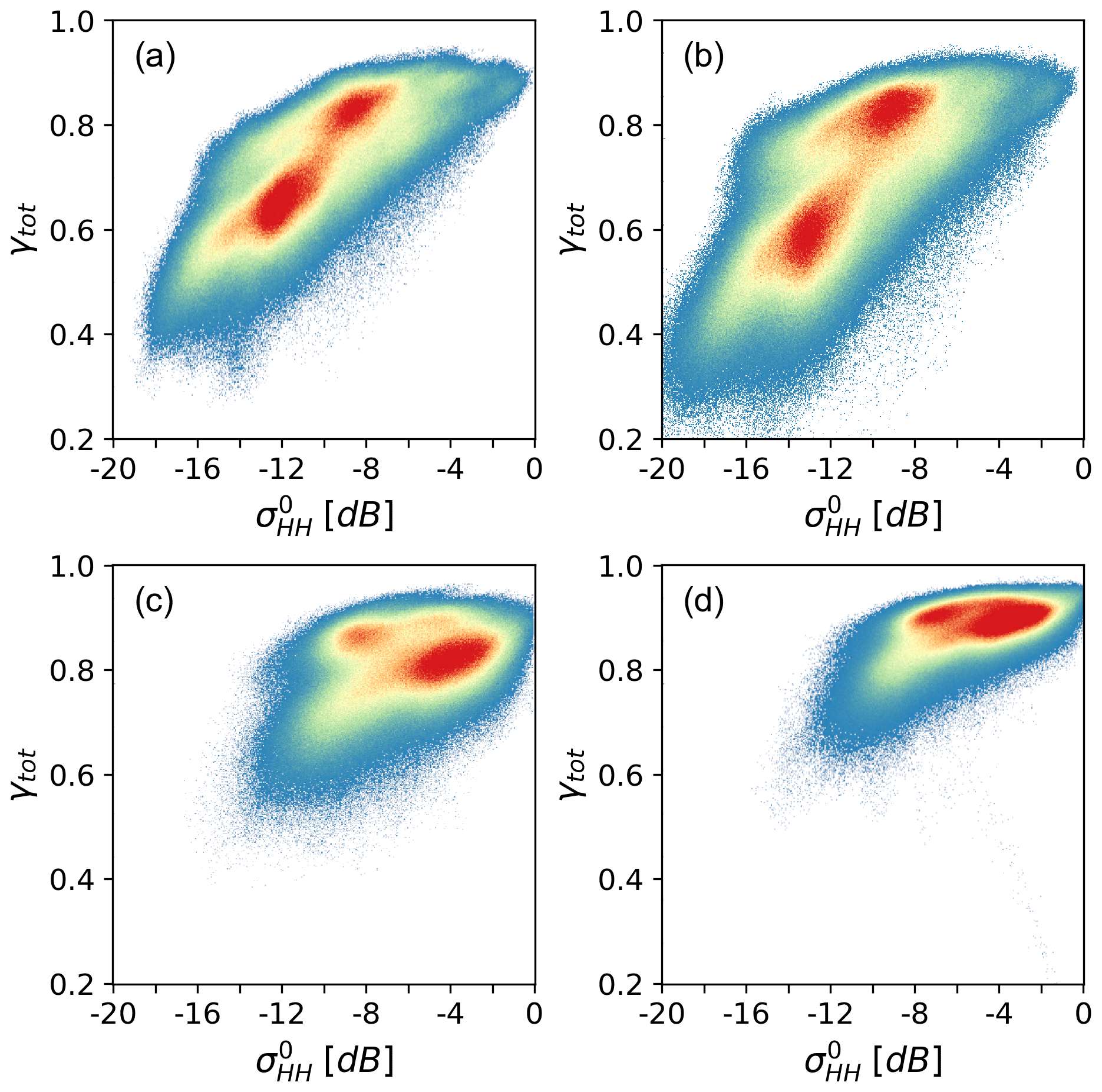
Figure 6 Scatterplot of the backscatter coefficient σ^∘_HH (dB) vs. the total normalised coherence, γ_tot, in the AoI. (a) 6 May 2013 (θ_i=40.9^∘), (b) 22 May 2013 (θ_i=38.6^∘), (c) 10 December 2016 (θ_i=21.6^∘), (d) 10 January 2018 (θ_i=21.1^∘). The colour represents the 2D data density increasing from blue to red. The reduced range of coherence in (d) compared to (c) can be attributed to the shorter effective baseline.

The coherence image of 6 May 2013 (Fig. 4) shows the lowest coherence on glacier sections with the largest elevation bias located on Driscoll Glacier and near the ALE camp (γ_tot=0.50 to 0.65). In the T2013 and T2014 (T2013/14) TDM images, the coherence of the BIA is also comparatively low (mean γ_tot=0.79) because of thermal decorrelation due to the low SNR. In the low-accumulation areas surrounding the BIA the σ^∘ values range from −5 to −8 dB, and the magnitude of γ_tot ranges from 0.85 to 0.90. The incidence angle also has an impact on the relation between coherence and σ^∘. This is evident by comparing scatterplots of scenes with different incidence angles (Fig. 6). The two scenes with incidence angles of 40.9 and 38.6^∘, respectively, show an approximately linear relation between coherence and σ^∘, with two cluster centres corresponding to the surroundings of the BIA and to areas with higher accumulation rates, respectively. The scenes with a 22^∘ incidence angle (T2016/18) show reduced dynamic range of coherence and σ^∘. The volumetric normalised coherence, derived from the observed total coherence according to Eq. (3), shows the expected trend, i.e. decrease in γ_Vol with increasing baseline (decreasing H_a) at a given incidence angle (Table 3). The lowest mean coherence value over the AoI is observed for scene T2014A ($\left|H_{\mathrm{a}}\right|=\mathrm{42.9}$ m, γ_Vol=0.656).

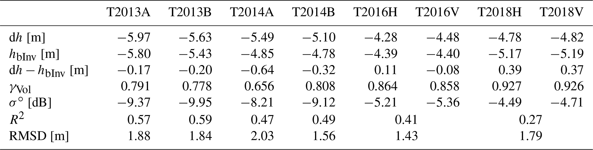
Table 3 Mean values over the AoI for the elevation difference TDM − REMA (dh), the TDM elevation bias by inversion of volumetric coherence (h_bInv), the difference between dh and h_bInv, the volumetric coherence (γ_Vol), and the backscatter coefficient (σ^∘). R² is the coefficient of determination for linear correlation between d_h and h_bInv; RMSD is the root mean square difference between d_h and h_bInv.

4.3 Backscatter signatures, coherence and elevation bias at the snow pit sites

The backscatter coefficients, the magnitude of the total and volumetric correlation coefficients and the elevation bias for cells with 90 m diameter centred at the snow pit sites are listed in Tables S3 and S4. The speckle-related uncertainty (standard deviation) of σ^∘ for the 90 m cells is 0.13 dB for the single-polarised data at θ_i=40^∘ (T2013/14 scenes) and 0.26 dB for the HH- and VV-polarised data at θ_i=22^∘ (T2016/18 scenes). The γ values are based on the coherence pixels whose centre coordinates fit within the corresponding 90 m cell. Pit 5 is not covered by the scenes T2016 (10 December 2016) and T2018 (10 January 2018). We derived the data for pit 5 from two scenes of adjoining tracks with similar height of ambiguity and incidence angle: 7 January 2017 (θ_i=24.6^∘, $H_{\mathrm{a}}=-\mathrm{70.0}$ m) and 16 January 2018 (θ_i=24.7^∘, $H_{\mathrm{a}}=-\mathrm{106.0}$ m).

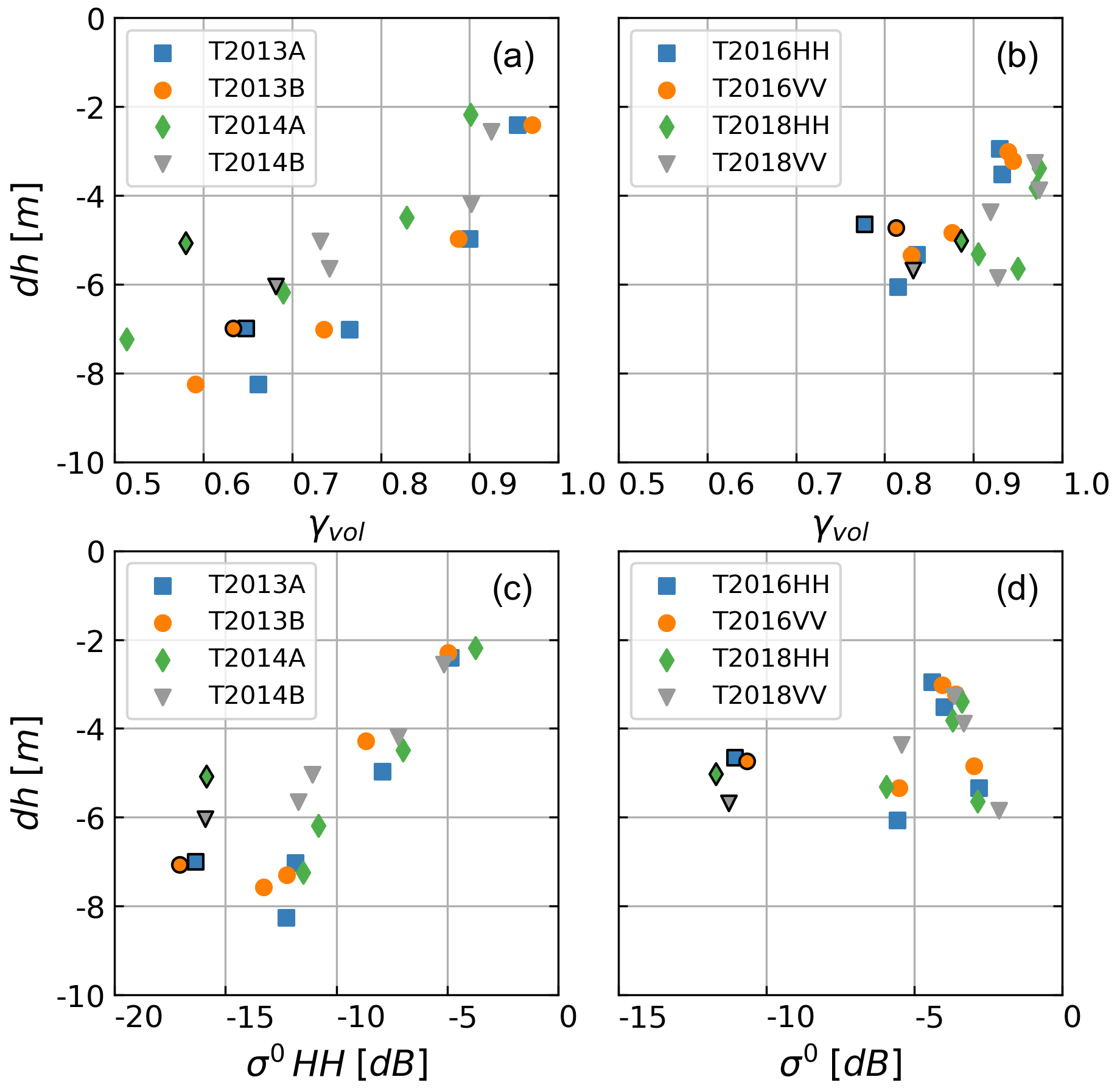
Figure 7 Relations between the elevation difference (dh) TDM − REMA and volumetric coherence (a, b) as well as between the elevation difference and the backscatter coefficient (c, d) for the snow pit sites P1 to P5. The framed points refer to P5. Incidence angle in the swath centre: (a, c) θ_i=37.5 to 40.9^∘, (b, d) θ_i=21.6 and 22.1^∘.

Figure 7 shows plots of the volumetric coherence and the backscatter coefficient versus the elevation difference dh between the TDM DEMs and the REMA at the snow pit sites. In order to point out effects of the incidence angle, the data derived from the T2013/14 and from the T2016/18 scenes are displayed separately. There is a clear trend of decrease in γ_Vol with increasing magnitude of dh. The scene T2014A with the largest $\left|H_{\mathrm{a}}\right|$ shows the highest sensitivity of γ_Vol with respect to dh, and the scene T2018 with the shortest $\left|H_{\mathrm{a}}\right|$ shows the lowest sensitivity.

The incidence angle also has an effect on the elevation bias. For example, the two scenes with almost the same height of ambiguity show different mean dh values of the snow pit sites (Table S4) – T2013A: $\left|H_{\mathrm{a}}\right|=\mathrm{65.6}$ m, 〈dh〉=5.93 m; T2016: $\left|H_{\mathrm{a}}\right|=\mathrm{67.3}$ m, 〈dh〉=4.35 m. The same behaviour is evident for the mean dh of the AoI (Table 3): 〈dh〉=5.97 m for T2013A and 〈dh〉=4.38 m for T2016.

Regarding polarisation, there are no significant differences between HH- and VV-polarised data for γ_Vol and dh. Whereas the snow pit sites show slightly larger $\left|\mathrm{d}h\right|$ at HH polarisation, over the AoI this is the case at VV polarisation. The differences in σ^∘ and coherence between HH and VV polarisation are also small. The average σ^∘_HH of the snow pit sites is 0.28 dB lower than σ^∘_VV.

The plots of dh vs. σ^∘ at the snow pits in Fig. 7 indicate for the T2013/14 scenes an approximately linear relation for the sites P1 to P4, but the data of P5 (〈σ^∘$\rangle =-\mathrm{16.3}$ dB) are shifted by a few decibels. The reduced σ^∘ of P5 can be attributed to the smaller grain size and a smoother vertical density profile. The T2016/18 data do not show any obvious relation between dh and σ^∘. P4 (σ^∘ HH −2.8 dB) and P5 (σ^∘ HH −11.0 dB) have a similar elevation bias. The same behaviour as for P4, comparatively deep penetration and high σ^∘ in the T2016/18 data, is evident for an extended area in its surroundings which shows high backscatter in the T2016/18 data (mean σ^∘ = −3 dB) and a comparatively large elevation bias (mean dh = −5 m). The high σ^∘ at near-nadir angles is an indication of increased backscatter at internal interfaces, but it is not clear why this has less impact on volume decorrelation.

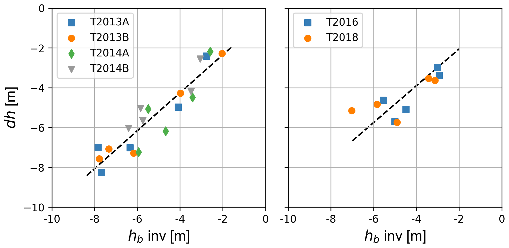
Figure 8 Elevation difference (dh) TDM DEM − REMA versus the computed elevation bias, derived from the volumetric coherence for the snow pit sites P1 to P5. The dashed line is the linear regression line.

5 Estimation of the interferometric elevation bias

Building on the signature analysis reported in Sect. 4, we focus on the use of the volumetric coherence for estimating the interferometric elevation bias by inverting γ_Vol according to Eq. (12). For computing the vertical wavenumber in the volume and the refraction angle, we assume a snow density of 400 kg m⁻³, resulting in ${\mathit{\epsilon }}^{\prime }=\mathrm{1.763}$ (Mätzler, 1996). Figure 8 shows plots of the computed elevation bias, h_bInv, at the snow pit sites derived from γ_Vol vs. the elevation difference dh between the InSAR DEMs and the REMA. The T2013/14 data show a highly significant linear relation between dh and h_bInv, with a coefficient of determination R²=0.86. The root mean square difference (RMSD) is 0.74 m, attributed to errors in the computed h_bInv and the DEM difference product. The T2016/18 data (mean of HH and VV polarisation) show a linear relation with R²=0.59 and RMSD = 0.84 m.

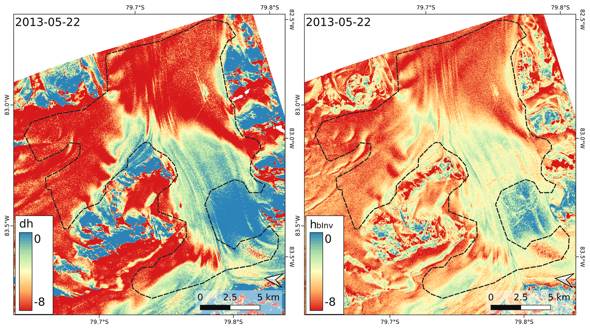
Figure 9 Elevation difference (dh) TDM DEM − REMA and elevation bias (h_bInv) by inversion of γ_Vol for the TDM scene on 22 May 2013 (θ_i=38.6^∘). The outline encloses the AoI.

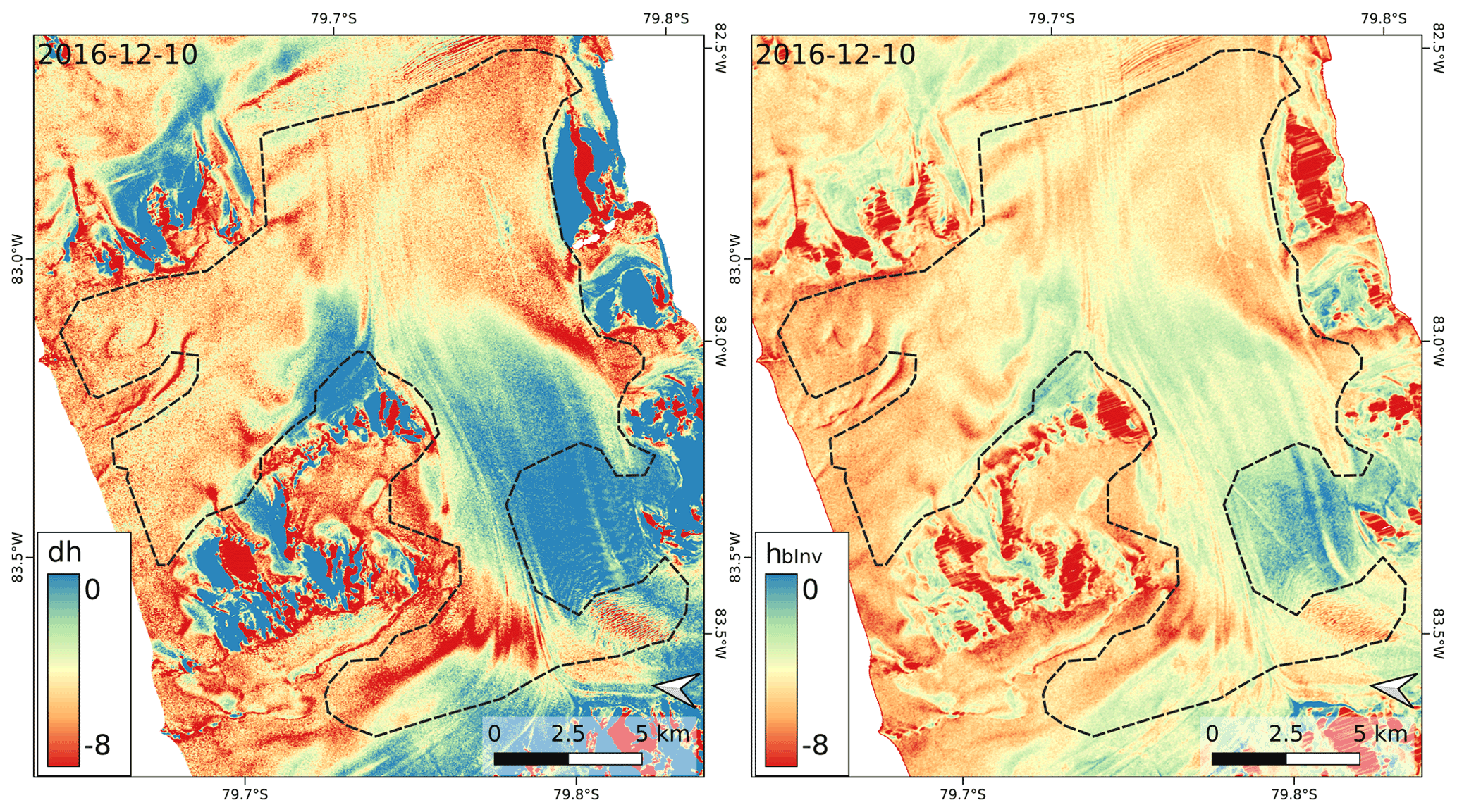
Figure 10 Elevation difference (dh) TDM DEM − REMA and elevation bias (h_bInv) by inversion of γ_Vol for the TDM scene on 10 December 2016 (θ_i=21.6^∘), based on HH- and VV-polarised data.

Maps of dh and the computed TDM elevation bias are shown in Fig. 9 for scene T2013B and in Fig. 10 for scene T2016. These two scenes have almost the same vertical wavenumber but different incidence angles. The differences between HH- and VV-polarised data of the T2016 and T2018 scene, respectively, are insignificant. We use the mean value of the HH- and VV-based DEMs of the single dates for the comparison in order to reduce the impact of random phase noise. In Table 3 mean numbers over the AoI are specified for dh, h_bInv, γ_Vol, the coefficient of determination (R²) for linear correlation between dh and h_bInv, and the RMSD. The numbers for R² and RMSD refer to the maps resampled to 8 m grid size, low-pass filtered over 7×7 pixels windows using a Gaussian function. The dh value of the TDMgl DEM (dh = 5.61 m) differs only by 0.06 m from the mean dh of the T2013/14 data. The TDMgl DEM is based on several TDM scenes acquired in 2013 and 2014. The dh map for TDMgl vs. REMA shows a similar spatial pattern as dh of the individual DEMs (Fig. S2).

As for the snow pit sites, the mean values over the AoI show distinct differences in dh, h_bInv and γ_Vol between the data sets with different incidence angles. The magnitudes of the elevation bias of the T2013/14 data (mean dh $=-\mathrm{5.55}$ m, $h_{\mathrm{bInv}}=-\mathrm{5.22}$ m) are larger than the corresponding values of the T2016/18 data set (dh $=-\mathrm{4.59}$ m, $h_{\mathrm{bInv}}=-\mathrm{4.79}$ m). As for the snow pit sites, this is opposite to the expectation for a uniform isotropic scattering medium for which $\left|h_{\mathrm{b}}\right|$ should be larger in scenes with smaller off-nadir angles in the case of the same value of H_a.

The AoI mean values of dh and h_bInv show minor differences: −0.33 m for T2013/14 and 0.20 m for T2016/18. The spatial patterns of dh and h_bInv are similar, but the mean slope of the 2D distribution deviates from the 1:1 correspondence (Fig. 11). The magnitude of the computed elevation bias is overestimated over the areas with coarse-grained firn and small penetration depth in the surroundings of the BIA and underestimated in areas of higher accumulation rate. These depth-dependent deviations can, at least partly, be attributed to the simplified assumption of the uniform volume approach.

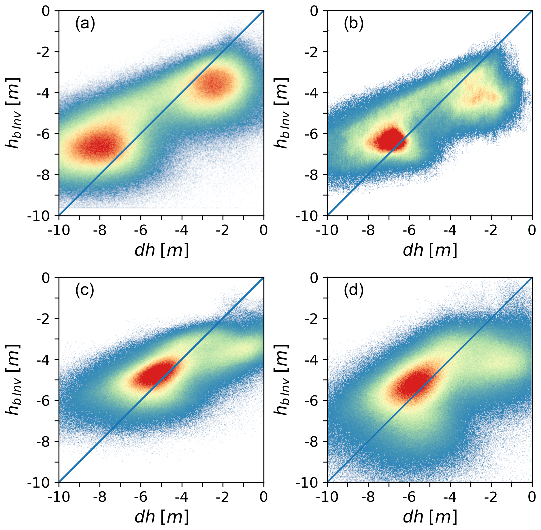
Figure 11 Scatterplot of the elevation difference TDM DEM minus REMA (dh) vs. the computed elevation by inversion of γ_Vol (h_bInv) in the AoI. (a) TDM scene on 22 May 2013, (b) mean of the T2013 and T2014 scenes, mean values of VV and HH channels on (c) 10 December 2016 and (d) 10 January 2018. The line shows the 1:1 correspondence. The colour code represents the 2D data density.

6 Discussion

A critical issue for inverting interferometric coherence in terms of the InSAR elevation bias is the description of the vertical backscattering profile in the snow volume. A simple model is required, in particular if only single-channel backscatter data are available. We apply the model of Dall (2007), in which the vertical backscatter function is defined by the extinction coefficient of a uniform random volume accounting for the combined effect of absorption and scattering. In order to check the suitability of this model for describing the backscattering profile of layered polar firn, we performed backscatter simulations for the snow pit sites with a multilayer radiative transfer model (Appendix A).

The computed total σ^∘ values at θ_i=40^∘ are matching the observed total backscatter intensities of the T2013/14 scenes for snow pit sites 2 to 5. The simulated vertical backscatter profiles and the exponential profiles of the uniform volume approach show close agreement for sites 2 to 4. The variations between individual layers, tracing back to accumulation and wind erosion events as well as to seasonal effects, are suppressed in the vertical profile of the cumulative backscatter contributions. At sites 2 to 4 the uniform volume approach shows minor overestimation of the backscatter contributions from the top snow layers due to the assumption of a constant scattering coefficient, whereas the actual grain size in the near-surface layers is below average. This effect is more pronounced at pit 5, where the layers with small grains reach down to 1.4 m depth.

On the other hand, the radiative transfer simulations at θ_i=22^∘, referring to the T2016/18 scenes, yield underestimation of σ^∘ by several dB. For pit 1 the simulated backscatter intensity is underestimated also at θ_i=40^∘. The incidence angle differences (Fig. 5) are most pronounced in the glacier zones with comparatively high accumulation. The radiative transfer model used for the simulations computes volume scattering for bi-continuous, random structures applying the improved Born approximation and assumes plane-parallel, homogenous layers (Picard et al., 2018). As a matter of fact, in addition to incoherent volume scatter, the contributions of rough internal interfaces as well as interlayer interferences play a role (Tan et al., 2017; Fischer et al., 2019b).

The most likely explanation for the increased backscatter towards near-nadir incidence is the increased scattering at interfaces between layers of different density and wind-packed structures. In particular on the main section of Union Glacier the snow surfaces are wind-roughened, showing elongated sastrugi at the metre scale and vertical roughness on the order of several centimetres. The surface roughness related to wind packing and erosion is also evident in snow pits at interfaces between snow layers and at wind crusts. Ashcraft and Long (2006) attribute the backscatter anisotropy, observed in scatterometer data of katabatic wind zones, to the anisotropy in the preferential roughness direction of the snow surface and of internal interfaces. Such behaviour was also observed for density-stratified firn on the East Antarctic Plateau and reproduced by simulations with a layered-medium radiative transfer model (Rott et al., 1993; West et al., 1996).

Whereas differential propagation effects lead to distinct co-polarisation differences in the phase and magnitude of the complex co-polarised (HH–VV) coherence, the differences in the interferometric coherence and derived penetration bias between the individual polarisations are insignificant (Table 3). This implies that the vertical backscatter distributions of the co-polarisation channels are similar. Consequently, the data from HH and VV polarisation can be combined for estimating the elevation bias, reducing the impact of noise. The differences in σ^∘ between HH and VV polarisation are also small, as to be expected for low-incidence-angle data (Fung, 1994). On average, over the AoI, σ^∘_HH is higher by 0.2 dB compared to σ^∘_VV, and there is no distinct spatial variability.

We also checked the information content of the phase, ϕ_HH−VV, and magnitude, $\left|{\mathit{\gamma }}_{\mathrm{HH}-\mathrm{VV}}\right|$, of the complex HH–VV-polarised correlation coefficient regarding potential contributions in support of elevation bias retrievals. Measurements with a ground-based (Jordan et al., 2019) and an airborne (Dall, 2009) polarimetric ice sounder in the dry-snow zone of Greenland show major variations in ϕ_HH−VV related to anisotropic scattering at internal interfaces and to the crystal orientation of ice fabrics. Leinss et al. (2016) derived ϕ_HH−VV from TerraSAR-X and ground-based scatterometer data in order to determine the dielectric and structural anisotropy of seasonal snow, showing distinct differences in ϕ_HH−VV related to the snow microstructure. We computed the complex co-polarised correlation coefficient from data of the T2016 scene using estimation windows comprising about 125 independent samples (Fig. S3). The co-polarised coherence, $\left|{\mathit{\gamma }}_{\mathrm{HHVV}}\right|$, reflects to some degree the spatial pattern of the elevation bias. In the BIA $\left|{\mathit{\gamma }}_{\mathrm{HH}-\mathrm{VV}}\right|$ is 0.92, in the low-accumulation areas near the BIA 0.6 to 0.7, and in the vicinity of the ALE camp 0.3 to 0.5. In the AoI the linear correlation coefficient, R², between $\left|{\mathit{\gamma }}_{\mathrm{HH}-\mathrm{VV}}\right|$ and dh amounts to 0.29. Reduced coherence can be attributed to decorrelation by the non-coherent scattering components in the volume.

The mean co-polarised phase difference, ϕ_HH−VV, of the BIA is close to zero (0.05 rad), as to be expected for backscatter from a comparatively smooth surface. In the AoI (snow and firn) the mean value of ϕ_HH−VV amounts to 0.50 rad with a high standard deviation (0.39 rad) because the ensemble comprises positive as well as negative values. Positive phase differences, an indication of anisotropic scattering at horizontal structures such as internal interfaces, are dominating on the main glacier. A substantial part of Driscoll Glacier shows negative ϕ_HH−VV values, the reason for which is unclear. In the AoI the correlation coefficient R² between ϕ_HH−VV (comprising positive and negative values) and dh is close to zero, whereas R² for the magnitude of the phase difference, $\left|{\mathit{\varphi }}_{\mathrm{HH}-\mathrm{VV}}\right|$, is 0.19. These observations are an indication of differential propagation effects between HH- and VV-polarised waves in the snow–firn volume, but the sources of the anisotropy are not uniquely defined. In order to assess the value of the complex co-polarised correlation coefficient for supporting retrievals of the penetration-related elevation bias, dedicated studies are needed, employing preferably multi-incidence angle observations.

According to theory the penetration bias and phase centre depth at a given frequency and polarisation change with the baseline and the incidence angle (Dall, 2007). This was verified with airborne data by Fischer et al. (2020), showing that the changes are significant in particular at small volumetric wavenumbers (long baselines). This is evident comparing two scenes with almost the same incidence angle: T2016 (θ_i=21.6^∘, k_zVol=0.120) and T2018 (θ_i=22.1^∘, k_zVol=0.072). Both the dh and h_bInv values indicate deeper penetration for T2018 compared to T2016, amounting in the AoI to dh = −4.80 m for T2018 versus −4.38 m for T2016 and to $h_{\mathrm{bInv}}=-\mathrm{5.18}$ m for T2018 versus −4.40 m for T2016 (Table 3).

For a uniform scattering medium, deeper penetration is expected for a steeper propagation path (lower incidence angle). This can be checked by comparing two scenes with almost the same vertical wavenumber and different incidence angles: T2013B (θ_i=38.6^∘, k_zVol=0.121, dh(AoI) = −5.63 m) and T2016 (θ_i=21.6^∘, k_zVol=0.120, dh(AoI) = −4.38 m). However, assuming for T2016 a volume with the same scattering and absorption coefficients as for T2013B, the expected elevation bias for T2016 is −6.04 m. The same behaviour is evident for the mean dh values of the snow pit sites: $\langle \mathrm{d}h\rangle =-\mathrm{5.70}$ m for T2013B, $\langle \mathrm{d}h\rangle =-\mathrm{4.35}$ m for T2016. This mismatch also points to increased scattering at internal interfaces at low incidence angles, as concluded from backscatter modelling (see Appendix A).

The impact of the incidence angle on the mean discrepancy between the observed dh and the computed h_bInv is comparatively small. For T2103/14 the mean value for dh − h_bInv amounts to −0.33 m, for T2016/18 to 0.20 m (Table 3). This shows that the uniform volume approach, based on the volumetric coherence, delivers on average reasonable penetration corrections. However, biases for deep and shallow penetration, respectively, indicate systematic deviations from the uniform volume approach. In the first case the smaller grain size of the top snow layers causes a shift in the scattering phase centre to larger depth compared to exponential extinction. The second case, an overestimation of h_b in wind-exposed low-accumulation zones, can be attributed to the larger size of the scattering elements and a denser sequence of internal interfaces.

7 Conclusion

In this study we investigated the feasibility for estimating the penetration-related elevation bias of interferometric topographic products over snow and ice by inverting the volumetric coherence. Single-pass across-track SAR interferometry has been widely applied for comprehensive, spatially detailed measurements of glacier and ice sheet topography as the measurements are not impaired by temporal decorrelation of the interferometric signal, variations in atmospheric propagation conditions, cloudiness and variable illumination. A main concern for the use of InSAR DEMs over glaciers and ice sheets is the correction of the elevation bias. A common approach is the use of laser altimetry data as a reference for vertical co-registration (e.g. Abdullahi et al., 2019; Rizzoli et al., 2017a, b; Wessel at al., 2016). However, altimetry data often lack the required temporal coincidence and coverage for comprehensive corrections.

We applied and evaluated the method of Dall (2007) for deriving the elevation bias of dry polar snow and firn by inverting the volumetric coherence of X-band InSAR data of the TanDEM-X mission. This method is based on the assumption of a uniform volume with constant scattering and absorption properties, whereas actual snow–firn volumes show depth-dependent changes in the density and the scattering elements as well as variations at a small vertical scale related to stratification. The use of a simple model is required because the inversion of a single parameter does not allow the representation of the complex layered structure. The study area, Union Glacier in Antarctica, comprises ice-free surfaces, bare ice, dry snow and firn with different structural properties depending on wind exposure and accumulation, a suitable environment for studying the performance of the inversion algorithm. For the statistical analysis we focussed on level glacier areas, including sites of field measurements, in order to minimise the impact of possible errors in SAR image co-registration with optical reference data.

The TanDEM-X data set comprises interferometric pairs with different interferometric baselines as well as with two distinctly different incidence angle ranges. This enables us to study the impact of these parameters on the computed elevation bias. In spite of the simplified representation of the vertical backscatter profile, the inversion according to the model of Dall (2007) provides reasonable estimates. The mean values of the computed elevation bias over the level glacier area, derived from data of the different TDM scenes, range from −4.4 to −5.8 m, varying with the baseline and incidence angle. The mean differences between the computed penetration bias and the estimates based on differencing of optical and TDM DEMs range from 0.38 to −0.64 m for the different scenes. There is a trend for overestimation of the elevation bias in areas that are subject to high wind exposure and low accumulation rates and for underestimation in areas with higher accumulation. In both cases deviations from the uniform volume structure are the main reason. In the first case the dense sequence of horizontal structures related to internal wind crusts, ice layers and density stratification causes increased scattering in the near-surface layers. In the second case the smaller grain size of the top snow layers causes a downward shift in the scattering phase centre compared to the uniform volume approach.

Advancements for the estimation of the InSAR elevation bias can be expected from progress in the representation of snow–firn structural properties in models for radar signal propagation. After all, the derivation of the interferometric elevation bias from volumetric coherence is a promising option which should be carried forward as it delivers spatially detailed information coinciding in both space and time with the topographic products. Fischer et al. (2020) analysed deviations from the uniform volume approach for airborne multi-frequency polarimetric SAR data. They explored sources and interaction mechanisms responsible for these deviations and tested different models for vertical backscatter contributions, concluding that in the case of single-polarisation data the inversion based on the uniform volume model is a preferred approach. Beyond that, Fischer at al. (2019a) demonstrated the added value of multi-baseline polarimetric InSAR data for deriving the depth of dominant scattering layers in polar firn, key information for locating the position of the scattering phase centre within the volume. Consequently, further progress on InSAR signal penetration in layered media can be expected from the use of polarimetric data as well as from multi-baseline and multi-angle observations.

Appendix A: Representation of the vertical backscatter profile

In order to assess the suitability of the vertical backscatter distribution of the uniform volume approach, we performed backscatter simulations with a multilayer radiative transfer (RT) model. According to the RT theory the normalised radar cross-section scattered back from depth z of a random scattering medium and received at the surface can be described by

$$\begin{array}{}\text{(A1)}& {\mathit{\sigma }}^{\mathrm{0}}\left(z\right)=T^{\mathrm{2}}\left({\mathit{\theta }}_{\mathrm{i}}\right){\mathit{\sigma }}_{\mathrm{v}}^{\mathrm{0}}\left(z\right)\exp \left\{\mathrm{2}\underset{z}{\overset{\mathrm{0}}{\int }}\left[{\displaystyle \frac{k_{\mathrm{e}}\left(z\right)}{\cos {\mathit{\theta }}_{\mathrm{r}}}}\right]\mathrm{d}z\right\}.\end{array}$$

T is the transmissivity at the air–snow interface, ${\mathit{\sigma }}_{\mathrm{v}}^{\mathrm{0}}$ is the volume-scattering coefficient, k_e is the volume extinction coefficient accounting for scattering and absorption losses, θ_i is the incidence angle at the surface, θ_r is the refracted incidence angle, and z within the medium is negative. The factor 2 accounts for the two-way travel path in the volume. The uniform volume approach assumes constant scattering and extinction properties (Hoen and Zebker, 2000). The resulting vertical backscatter function, accounting for two-way losses, is given by

$$\begin{array}{}\text{(A2)}& {\mathit{\sigma }}^{\mathrm{0}}\left(z\right)=\langle {\mathit{\sigma }}_{\mathrm{v}}^{\mathrm{0}}\rangle \exp \left({\displaystyle \frac{\mathrm{2}z{k}_{\mathrm{e}}}{\cos {\mathit{\theta }}_{\mathrm{r}}}}\right)=\langle {\mathit{\sigma }}_{\mathrm{v}}^{\mathrm{0}}\rangle \exp \left({\displaystyle \frac{\mathrm{2}z}{d_{\mathrm{p}}}}\right),\end{array}$$

where $\langle {\mathit{\sigma }}_{\mathrm{v}}^{\mathrm{0}}\rangle$ is the average normalised volume-scattering cross-section, and d_p is the one-way power penetration depth.

We performed backscatter simulations for the snow pit sites with the multilayer Snow Microwave Radiative Transfer (SMRT) thermal emission and backscatter model of Picard et al. (2018). The SMRT offers a choice of different electromagnetic and microstructure models for computing the scattering and absorption coefficients and the scattering phase function in a given layer. We used the Sticky Hard Sphere (SHS) model for characterising the microstructure and the improved Born approximation for computing volume scattering and absorption. Input parameters for describing the microstructure of each layer with the SHS model are the snow density, the temperature, the effective grain size and the stickiness. The effective grain size refers to the maximum axis length of the prevailing snow grains in each layer (Fierz et al., 2009). Down to the bottom of the snow pits the grain size and density data are based on the field measurements. The increase in snow density below is adopted from the density profile of the firn core GUPA-1 of Hoffmann et al. (2020). For estimating the increase in grain size with depth below snow pit depth we apply the grain growth model of Linow et al. (2012).

The stickiness parameter, τ, is used in the SHS model to account for sintering and clustering of snow grains, forming aggregates that are larger than individual grains. The collective scattering and wave interaction effects of the aggregates result in increased scattering compared to individual grains and show a different phase function with more forward scattering. Löwe and Picard (2015) found stickiness to be an essential parameter when modelling snow as a sphere assembly. They show that the stickiness parameter can be objectively estimated from micro-tomography images. However, objective methods for deriving the stickiness parameter from field observations are pending. Typical stickiness values for X-band backscatter simulation of coarse-grained metamorphic snow are τ=0.1, whereas τ=1.0 is similar to the non-sticky case (Chang et al., 2014). We use τ as a tuning parameter in order to match the average observed and the computed total backscatter intensity at the individual sites. The τ values range from τ=0.1 for layers with large grains and clusters to τ=0.2 for near-surface layers. The computations were performed down to 20 m depth. Contributions to total backscatter from the layers below are negligible because of the dense medium effect and the attenuation in the layers above.

Whereas the stickiness parameter accounts for increased scattering due to bonding, the close packing of particles introduces near-field interactions, causing reduced scattering (Tsang et al., 2013). Compared to the assumption of independent scattering elements, the scattering in a dense medium decreases with increasing volume fraction of the scatterers larger than about 0.2. We performed test runs with the dense medium RT model with the quasi-crystalline approximation of Mie scattering (DMRT-QMS) of Tsang et al. (2007) and Chang et al. (2014) using the same stickiness and grain size parameters as for the computations with the improved Born approximation approach of SMRT. The results of both models are in close agreement and point out that the parameterisation of snow microstructure is decisive for snow backscatter simulations.

Figure A1 Fraction of X-band HH-polarised power scattered back from the snow–firn volume below the depth z. Points: radiative transfer model computations for individual layers. Curve: model for exponential extinction. Input parameters refer to Union Glacier pit 2 (a), pit 3 (b), pit 4 (c) and pit 5 (d).

Figure A1 shows vertical profiles of the power scattered back from the volume below a specific depth as a fraction of the total power observed at the surface, for both multilayer RT modelling results and the uniform volume (UV) approach. The RT computations refer to θ_i=40^∘, the mean local incidence angle at the snow pit sites of the T2013/14 scenes. The extinction coefficient for the exponential UV function is based on the mean penetration depth, which is deduced from the mean elevation difference (dh) between the T2013/14 scenes and the REMA assuming that the two-way penetration depth is equal to the elevation bias.

Layers with coarse grains and grain clusters show higher backscatter coefficients but are thinner than compact layers of higher density such as wind slabs. The variations between individual layers with different scattering properties are smoothed out in the depth-dependent backscatter function. Consequently, the exponential function is able to reproduce the vertical backscatter profiles quite well. The reduced backscatter contributions from near-surface layers shown by the RT model can be attributed to the smaller grain size, whereas the UV model assumes a constant scattering cross-section. This effect yields for pits 2, 3 and 4 only minor differences between the two models. At pit 5 the differences are more pronounced due to the smaller grain size of the top layers related to the higher accumulation rate.

The RT simulations for θ_i=40^∘, using τ as a tuning parameter, reproduce exactly the observed total mean backscatter intensity of the corresponding T2013/14 data at snow pit sites 2 to 5. For pit 1 the simulations for θ_i=40^∘ yield an underestimation of 3 dB, even when assuming consistently maximum stickiness (τ=0.1), very likely due to neglect of the enhanced scattering contributions of ice layers and wind crusts. The RT simulations for θ_i=22^∘, corresponding to the T2016/18 incidence angle, show underestimation throughout. The simulations for pit 2 to pit 5 show for incidence angles from 40 to 22^∘ an average σ^∘ increase of 1.3 dB, whereas the observed average increase is 5.9 dB. Large incidence angle dependence of backscatter is typical for density-layered firn. Ground-based X-band scatterometer measurements at several sites in the dry-snow zone of Dronning Maud Land with accumulation rates between 130 and 260 kg m⁻² a⁻¹, comparable to those on Union Glacier, show for incidence angles from 40 to 20^∘ a mean σ^∘ increase of 6.5 dB (Rott et al., 1993). The strong increase towards low off-nadir angles is an indication of increased scattering at horizontal structures such as rough interfaces between snow layers of different density and wind crusts, whereas the RT model assumes plane-parallel layered structures.